Avoiding tipping points in fisheries management through Gaussian Process Dynamic Programming

Abstract

Model uncertainty and limited data are fundamental challenges to robust management of human intervention in a natural system. These challenges are acutely highlighted by concerns that many ecological systems may contain tipping points, such as Allee population sizes. Before a collapse, we do not know where the tipping points lie, if they exist at all. Hence, we know neither a complete model of the system dynamics nor do we have access to data in some large region of state-space where such a tipping point might exist. We illustrate how a Bayesian Non-Parametric (BNP) approach using a Gaussian Process (GP) prior provides a flexible representation of this inherent uncertainty. We embed GPs in a Stochastic Dynamic Programming (SDP) framework in order to make robust management predictions with both model uncertainty and limited data. We use simulations to evaluate this approach as compared with the standard approach of using model selection to choose from a set of candidate models. We find that model selection erroneously favors models without tipping points – leading to harvest policies that guarantee extinction. The GPDP performs nearly as well as the true model and significantly outperforms standard approaches. We illustrate this using examples of simulated single-species dynamics, where the standard model selection approach should be most effective, and find that it still fails to account for uncertainty appropriately and leads to population crashes, while management based on the GPDP does not, since it does not underestimate the uncertainty outside of the observed data.

Introduction

Decision making under uncertainty is a ubiquitous challenge in the management of human intervention in natural resources and conservation. Decision-theoretic approaches provide a framework to determine the best sequence of actions in face of uncertainty, but only when that uncertainty can be meaningfully quantified (Fischer et al. 2009). Over the last four decades (beginning with Clark (1976), Clark (2009) and Walters and Hilborn (1978)) dynamic optimization methods, particularly Stochastic Dynamic Programming (SDP), have become increasingly important as a means of understanding how to manage human intervention into natural systems. Simultaneously, there has been increasing recognition of the importance of multiple steady states or ‘tipping points’ (Scheffer et al. 2001, 2009, Polasky et al. 2011) in ecological systems.

We develop a novel approach to address these concerns in the context of fisheries; although the challenges and methods are germane to other problems of conservation or natural resource exploitation. Economic value and ecological concern have made marine fisheries the crucible for much of the founding work on management under uncertainty (Gordon 1954, Clark 1976, 2009, May et al. 1979, Reed 1979, Ludwig and Walters 1982).

Even if we know the proper deterministic description of the biological system, there is intrinsic stochasticity in biological dynamics, measurements, and implementation of policy (e.g. Reed 1979, Clark and Kirkwood 1986, Roughgarden and Smith 1996, Sethi et al. 2005). We may also lack knowledge about the parameters of the biological dynamics (parametric uncertainty, e.g. Ludwig and Walters 1982, Hilborn and Mangel 1997, McAllister 1998, Schapaugh and Tyre 2013), or even not know which model is proper description of the system (structural uncertainty, e.g. Williams 2001, Cressie et al. 2009, Athanassoglou and Xepapadeas 2012). Of these, the latter is generally the hardest to quantify. Typical approaches confront the data with a collection of models, assuming that the true dynamics (or reasonable approximation) is among the collection and then use model choice or model averaging to arrive at a conclusion (Williams 2001, Cressie et al. 2009, Athanassoglou and Xepapadeas 2012). Even setting aside other concerns (see Cressie et al. (2009)), these approaches are unable to describe uncertainty outside the observed data range.

Structural uncertainty is particularly insidious when we try to predict outside of the range of observed data (Mangel et al. 2001) because we are extrapolating into unknown regions. In management applications, this extrapolation uncertainty is particularly important since (a) management involves considering actions that may move the system outside the range of observed behavior, and (b) the decision tools (optimal control theory, SDP) rely on both reasonable estimates of the expected outcomes and on the weights given to those outcomes (e.g. Weitzman 2013). Thus characterizing uncertainty is as important as characterizing the expected outcome.

Tipping points in ecological dynamics (Scheffer et al. 2001, Polasky et al. 2011) highlight this problem because precise models are not available and data are limited such as around high stock levels or an otherwise desirable state. With perfect information, one would know just how far a system could be pushed before crossing the tipping point, and management would be simple. But we face imperfect models and limited data and, with tipping points, even small errors can have very large consequences, as we shall illustrate later. Because intervention may be too late once a tipping point has been crossed (but see Hughes et al. (2013)), management is often concerned with avoiding tipping points before any data about them are available.

The dual concerns of model uncertainty and incomplete data create a substantial challenge to existing decision-theoretic approaches (Brozović and Schlenker 2011). We illustrate how Stochastic Dynamic Programming (SDP) (Mangel and Clark 1988, Marescot et al. 2013) can be implemented using a Bayesian Non-Parametric (BNP) model of population dynamics (Munch et al. 2005a). The BNP method has two distinct advantages. First, using a BNP model sidesteps the need for an accurate model-based description of the system dynamics. Second, a BNP model better reflects uncertainty when extrapolating beyond the observed data. This is crucial to providing robust decision-making when the correct model is not known (as is almost always true). [We use robust to characterize approaches that provide nearly optimal solutions without being sensitive to the choice of the (unknown) underlying model.]

This paper is the first ecological application of the SDP without an a priori model of the underlying dynamics. Unlike parametric approaches that can only reflect uncertainty in parameter estimates, the BNP method provides a broader representation of uncertainty, including uncertainty beyond the observed data. We will show that Gaussian Process Dynamic Programming (GPDP) allows us to find robust management solutions in face of limited data without knowing the correct model structure.

For comparisons, we consider the performance of management based on GPDP against management policies derived under several alternative parametric models (Reed 1979, Ludwig and Walters 1982, Mangel and Clark 1988). Rather than compare models in terms of best fit to data, we compare model performance in the concrete terms of the decision-maker’s objectives.

Approach and Methods

We first describe the requirements of dynamic optimization for the management of human intervention in natural resource systems. After that we describe three parametric models for population dynamics and the Gaussian Process (GP) description of population dynamics. All computer code used here has been embedded in the manuscript sources (see Xie (2013)), and an implementation of the GPDP approach is provided as an accompanying R package. Source code, R package and the CSV data files corresponding each figure are archived in the supplement (Boettiger et al. 2014).

Requirements of dynamic optimization

Dynamic optimization requires characterizing the dynamics of a state variable (or variables), a control action, and a value function. For simplicity, we consider only a single state variable. This is a best-case scenario for the parametric models because we simulate underlying dynamics from one of the three parametric models, whereas in the natural world we never know the “true” model. In addition, by choosing one-dimensional models with just a few parameters, we limit the chance that poor performance will be due to inability to estimate parameters accurately, something that becomes a more severe problem for higher-dimensional parametric models. Finally, the parametric models we consider are commonly used in modeling stock-recruitment dynamics or to model sudden transitions between alternative stable states.

We let $X(t)$ denote the size (numbers or biomass) of the focal population at time $t$ and assume that in the absence of take its dynamics are:

$$X(t+1)=Z(t)f(X(t),\mathbf{p})$$ (1)

Where Z(t) is log-normally distributed process stochasticity (Reed 1979) and $\mathbf{p}$ is a vector of parameters to be estimated from the data. We describe the three choices for $f(X(t),\mathbf{p})$ in the next section. The control action is a harvest or take, $h(t)$, measured in the same units as $X$, at time $t$. Thus, in the presence of take, the population size on the right hand side of Eqn 1 is replaced by $S(t)=X(t)-h(t)$.

To construct the value function, we consider a return when $X(t)=x(t)$ and harvest $h(t)=h$ denoted as the reward, $R(x(t),h)$. For example, if the return is the harvest at time $t$, then $R(x(t),h(t))=\min(x(t),h(t))$. We assume that future harvests are discounted relative to current ones at a constant rate of discount $\delta$ and ask for the harvest policy that maximizes total discounted harvest between the current time $t$ and a final time $T$. That is, we seek to maximize over choices of harvest $E[\sum_{t=0}^{T}R(X(t),h(t),t)\delta^{t}]$, where the state dynamics are given by Eqn 1 and $E$ denotes the expectation over future population states.

In order to find that policy, we introduce the value function $V(x(t),t)$ representing the total discounted catch from time $t$ onwards given that $X(t)=x(t)$. This value function satisfies an equation of SDP (Mangel and Clark 1988, Clark and Mangel 2000, Clark 2009 Mangel 2014),

$$V(x(t),t)=\max_{h(t)}\{R(h(t),x(t))+\delta\cdot\mathbf{\mathrm{E}}_{X(t+1)}\left[V(X(t+1),t+1)|x(t),h(t)\right]\}$$ (2)

where expectation is taken over all possible values of the next state, $X(t+1)$, and maximized over all possible choices of harvest, $h(t)$. That is, at time $t$, when population size is $x(t)$ and harvest $h(t)$ is applied, the immediate return is $R(h(t),x(t))$. When the sole source of uncertainty is the process stochasticity term, $Z$, and thus the expectation in Eqn 2 is equivalent to taking expectations over $Z(t)$. That is

$$\mathbf{\mathrm{E}}_{X(t+1)}\left[V(X(t+1),t+1)|x(t),h(t)\right]=\mathbf{\mathrm{E}}_{Z(t)}\left[V(Z(t)f(x(t)-h(t))|\mathbf{p}),t+1|x(t),h(t)\right]$$ (3)

where the population size after the take is $x(t)-h(t)$, which is then translated into $X(t+1)$ by Eqn 1 (that is, we replace $X(t+1)$ by $Z(t)f(x(t)-h(t)|\mathbf{p})$).

When the parameters governing the dynamics are also uncertain, we take the expectation over the posterior distribution for the parameters:

$$\mathbf{\mathrm{E}}_{X(t+1)}\left[V(X(t+1),t+1)|x(t),h(t)\right]=\mathbf{\mathrm{E}}_{\mathbf{p}|\mathrm{data}}\{\mathbf{\mathrm{E}}_{Z(t)|\mathbf{p},\mathrm{data}}\left[V(Z(t)f(x(t)-h(t)|\mathbf{p}),t)\right]\}$$ (4)

When the underlying population dynamics are unknown (the case of structural uncertainty), the function $f$ itself is uncertain and the expectation for the next state includes uncertainty in $f$ as well. That is

$$\mathbf{\mathrm{E}}_{X(t+1)}\left[V(X(t+1),t+1)|x(t),h(t)\right]=\mathbf{\mathrm{E}}_{\mathbf{p}|\mathrm{data}}\{\mathbf{\mathrm{E}}_{f,Z(t)|\mathbf{p},\mathrm{data}}\left[V(Z(t)f(x(t)-h(t)|\mathbf{p}),t)\right]\}$$ (5)

We consider the finite time problem with $T=$ 1000, which we solve using the standard value iteration algorithm (see Mangel and Clark 1988, Clark and Mangel 2000).

Parametric Models

We consider three candidate parametric models for the population dynamics: The Ricker model, the Allen model (Allen and Tanner 2005), and the Myers model (Myers et al. 1995), Eqns (6)-(8). In all three, we let $K$ denote the carrying capacity and $r$ the maximum per capita growth rate. The Ricker model has two parameters and the right hand side of Eqn 1 is

$$f(S(t)|r,K)=S(t)e^{r\left(1-\frac{S(t)}{K}\right)}$$ (6)

The Allen model has three parameters

$$f(S(t)|r,K,X_{c})=S(t)e^{r\left(1-\frac{S(t)}{K}\right)\left(S(t)-X_{c}\right)}$$ (7)

where $X_{c}$ denotes the location of the unstable steady state (i.e., the tipping point).

The Myers model also has three parameters:

$$f(S(t)|r,K,\theta)=\frac{rS(t)^{\theta}}{1+\frac{S(t)^{\theta}}{K}}$$ (8)

where $\theta=1$ corresponds to Beverton-Holt dynamics and $\theta$ > 2 leads to Allee effects and multiple stable states.

The Ricker model does not lead to multiple steady states. The Allen model resembles the Ricker dynamics with an added Allee effect parameter (Courchamp et al. 2008), below which the population cannot persist. The Myers model also has three parameters and contains an Allee threshold, but unlike the Ricker model saturates at high population size. The multiplicative log-normal stochasticity in Eqn 1 introduces one additional parameter $\sigma$ that must be estimated.

Because of our interest in management performance in the presence of tipping points, all of our simulations are based on the Allen model. The Allen model is thus the state of nature and is expected to provide the best-case scenario. The Ricker model is a reasonable approximation of these dynamics far from the Allee threshold (but lacks threshold dynamics), while the Myers model shares the essential feature of a threshold but differs in structure from the Allen model. Throughout, we refer to the “True” model when the underlying parameters are known without error, and refer to the “Allen” model when these parameters have been estimated from the sample data.

We consider a period of 40 in which data are obtained to estimate the parameters or the GP. This is long enough that the estimates do not depend on the particular realization, and longer times are not likely to provide substantial improvement. Each of the models is fit to the same data (Figure 1).

We inferred posterior distributions for the parameters of each model by Gibbs sampling (Gelman et al. (2003) implemented in R (R Core Team 2013) using jags, (Su and Masanao Yajima 2013)). We choose uniform priors for all parameters of the parametric models (See appendix Tables S1-S3; R code provided). We show one-step-ahead predictions of these model fits in Figure 1. We tested each chain for Gelman-Rubin convergence and results were robust to longer runs. For each simulation we also applied several commonly used model selection criteria (AIC, BIC, DIC, see Burnham and Anderson (2002)) to identify the best fitting model.

Additionally, we compute the maximum likelihood estimate (MLE, as we will refer to this model in the figures) of the parameters for the (structurally correct) Allen model. Comparing this to using the posterior distribution of parameters inferred from MCMC for the same model gives some indication of the importance of this uncertainty in the dynamic programming.

The Gaussian Process model

The core difference for our purpose between the estimated GP and the estimated parametric models is that the estimated GP model is defined explicitly in reference to the observed data. As a result, uncertainty arises in the GP model not only from uncertainty in the parameters, but is also increases in regions farther from the observed states, such as low population sizes in the example illustrated here. The estimated parametric models, by contrast, are completely specified by the parameters.

The use of GPs to characterize dynamical systems is relatively new (Kocijan et al. 2005), and was first introduced in the context ecological modeling and fisheries management in Munch et al. (2005b). GP models have subsequently been used to test for the presence of Allee effects (Sugeno and Munch 2013a), estimate the maximum reproductive rate (Sugeno and Munch 2013b), determine temporal variation in food availability (Sigourney et al. 2012), and provide a basis for identifying model-misspecification (Thorson et al. 2014). An accessible and thorough introduction to the formulation and use of GPs can be found in Rasmussen and Williams (2006).

A GP is a stochastic process for which any realization consisting of n points follows a multivariate normal distribution of dimension $n$. To characterize the GP we need a mean function and a covariance function. We proceed as follows.

As before, we assume that the data $X(t)$ are observed with process stochasticity around a mean function $g(X(t))$

$$X(t+1)=g(X(t))+\varepsilon,$$ (9)

where $\varepsilon$ are IID normal random variables with zero-mean and variance $\sigma^{2}$. Note that we have chosen to assume additive stochasticity. While we could consider log-normal stochasticity as in the parametric models, we make this choice to emphasize that the Gaussian process approach need not have structurally correct stochasticity to be effective.

In order to make predictions, we update the GP based on the observed set of transitions. To do so, we collect the time series of observed states into a vector of “current” states, $\mathbf{X}_{\textrm{obs}}=\{X(1),\dots,X(T-1)\}$ and a vector of “next” states $\mathbf{Y}_{\textrm{obs}}=\{X(2),\dots,X(T)\}$ where $T$ is the time of the final observation. Conditional on these observations, the predicted next state, $g(X_{p})$, for any given “current” state, $X_{p}$ follows a normal distribution with mean $E$ and variance $C$ determined using the standard rules for conditioning in multivariate normals, i.e.

$$E=K(X_{p},\mathbf{X}_{\textrm{obs}})\left(K(\mathbf{X}_{\textrm{obs}},\mathbf{X}_{\textrm{obs}})-\sigma\mathbf{I}_{n}\right)^{-1}\mathbf{Y}_{\textrm{obs}}$$ (10)

and

$$C=K(X_{p},X_{p})-K(X_{p},\mathbf{X}_{\textrm{obs}})\left(K(\mathbf{X}_{\textrm{obs}},\mathbf{X}_{\textrm{obs}})-\sigma\mathbf{I}\right)^{-1}K(\mathbf{X}_{\textrm{obs}},X_{p})$$ (11)

Here $\mathbf{I}_{n}$ is the $n$ by $n$ identity matrix (i.e. a matrix with ones down the diagonal and zeros elsewhere) and $K$ is the ‘covariance kernel.’ The covariance kernel controls how much influence one observation has on another. In the present application we use the squared-exponential kernel which, when evaluated over a pair of vectors, say $\mathbf{x}$ and $\mathbf{y}$, generates a covariance matrix whose $i,j$th element is given by

$$K_{i,j}(\mathbf{x},\mathbf{y})=\exp\left(\frac{-(x_{i}-y_{j})^{2}}{2\ell^{2}}\right)$$ (12)

so that $\ell$ gives the characteristic length-scale over which correlation between two observations decays. See Rasmussen and Williams (2006) for other choices of covariance kernels and their properties. Note that this simple formulation assumes a prior mean of zero. For the parameters we use inverse Gamma priors on both the length-scale $\ell$ and $\sigma$, thus for example

$$f(\ell;\alpha,\beta)=\frac{\beta^{\alpha}}{\Gamma(\alpha)}\ell^{-\alpha-1}\exp\left(-\frac{\beta}{\ell}\right)$$ (13)

For the prior on $\ell$, $\alpha=$ 10 and $\beta=$ 10. The prior on $\sigma$, $\alpha=$ 5 and $\beta=$ 5.

We use a Metropolis-Hastings Markov Chain Monte Carlo (Gelman et al. (2003)) to infer posterior distributions of the parameters of the GP (Figure S4, code in appendix). Since the posterior distributions differ substantially from the priors (Figure S4), most of the information in the posterior comes from the data rather than the prior belief.

The method of Gaussian Process Dynamic Programming (GPDP)

We derive the harvest policy from the estimated GP by inserting it into a SDP algorithm. Given the GP posteriors, we construct the transition matrix representing the probability of going to each state $X(t+1)$ given any current state $x(t)$ and any harvest $h(t)$ (See the function gp_transition_matrix() in the provided R package). Given this transition matrix, we use the same value iteration algorithm as in the parametric case to determine the optimal policy. In doing so, the uncertainty in the future state under the GP, $X(t+1)$, includes both process uncertainty (based on the estimation of $\sigma$) and structural uncertainty of the posterior collection of curves.

Results

Parametric and GP models for population dynamics

To ensure our results are robust to the choice of parameters, we will consider 96 different scenarios. To help better understand the process, we first describe in detail the results of a single scenario.

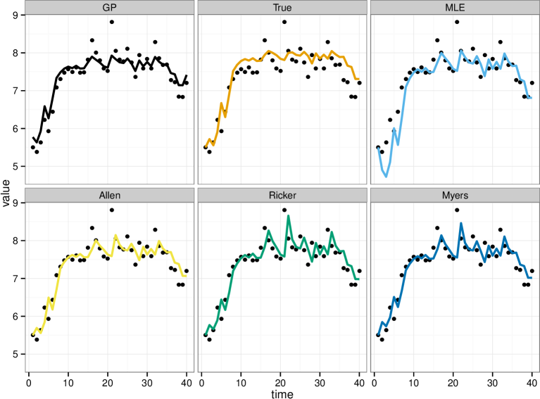
Figure 1: Points show the training data of stock-size over time. Curves show the expectations over the posterior step-ahead predictions based on each of the estimated models. Observe that all models are fitting the data reasonably well.)

All of the models fit the observed data rather closely and with relatively small uncertainty. In Figure 1, we show the posterior predictive curves. The training data of stock sizes observed over time are points, overlaid with the step-ahead predictions of each estimated model using the parameters sampled from their posterior distributions. Compared to the true model most estimates appear to over-fit, predicting patterns that are actually due purely to stochasticity. Model selection criteria (Table 1) penalize more complex models and show a preference for the simpler Ricker model over the models with alternative stable states (Allen and Myers). Supplement provides details on the model estimates.

Table 1: Model selection scores for several common criteria (DIC: Deviance Information Criterion, AIC: Akaike Information Criterion, BIC: Bayesian Information Criterion) all select the wrong model. As the true (Allen) model is not distinguishable from the simpler (Ricker) model in the region of the observed data, this error cannot be avoided regardless of the model choice criterion. This highlights the danger of model choice when the selected model will be used outside of the observed range of the data.

	Allen	Ricker	Myers
DIC	50.75	50.45	50.41
AIC	-24.51	-30.13	-27.01
BIC	-17.75	-25.06	-20.25

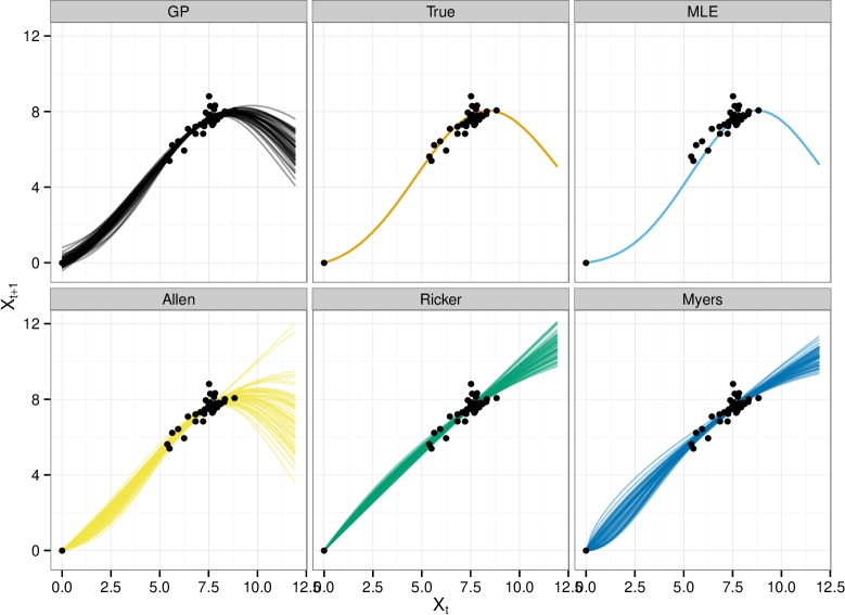
Figure 2: The inferred Gaussian process compared to the true process and maximum-likelihood estimated (MLE) process. We show the expected value for the function $f$ under each model. Plots show replicates drawn from the posterior distributions in order to convey uncertainty of the estimates. Note the MLE is a point estimate of parameters and so reflects no uncertainty in the distribution. The training data are also shown as black points. The GP is conditioned on (0,0), shown as a pseudo-data point.

We show the mean inferred population dynamics of each model relative to the true model used to generate the data in Figure 2, predicting the relationship between observed population size (x-axis) to the population size after recruitment the following year. In addition to the raw data, the GP is conditioned on going through the point 0,0 without error. All parametric models also make this assumption. Conditioning on (0,0) is equivalent to making the assumption that the population is closed, so that once it hits 0 it stays at 0, despite the lack of any data in the observed sequence to justify this. This assumption illustrates how the GP can capture common-sense biology without having to assume more explicit details about the dynamics at low population numbers that have never been observed. If the population were not closed, one could repeat the entire analysis without this assumption. Unlike parametric models, the GP corresponds to a distribution of curves, of which this plot only shows the means. Uncertainty in the parameters of the GP (not shown) further widens the band of possible population sizes. In Figure S1 (see supplement), we show the performance of the models outside the observed training data.

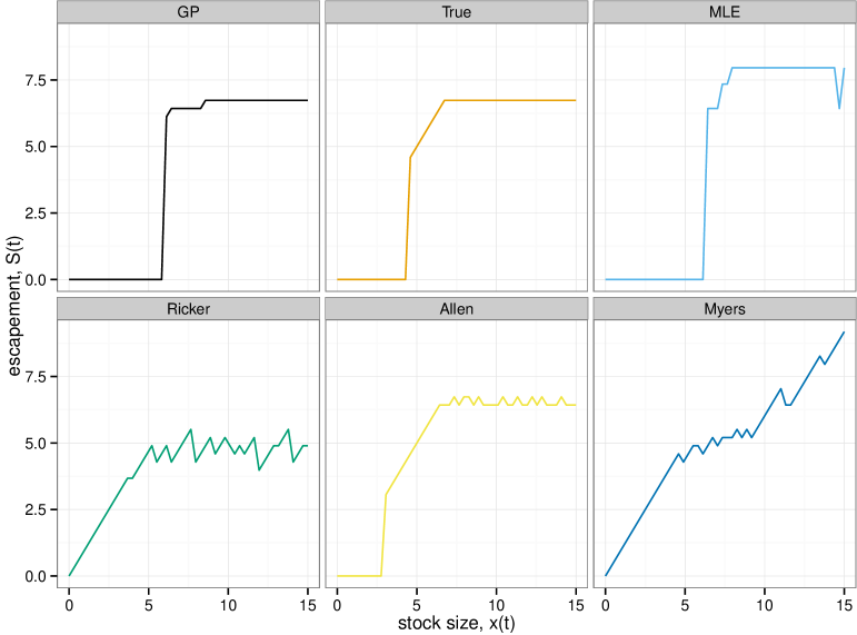
Figure 3: The steady-state optimal policy (infinite boundary) calculated under each model. Policies are shown in terms of target escapement, $S(t)$, as under models such as this a constant escapement policy is expected to be optimal (Reed 1979) Several policies show a numerical jitter due to the discretization of states in the dynamic programming algorithm; doubling the number of grid points did not qualitatively change the results.

Despite the similarities in model fits to the observed data, the policies inferred under each model differ widely (Figure 3). Policies are shown in terms of target escapement, $S(t)=x_{t}-h$. Under models such as this a constant escapement policy is expected to be optimal (Reed 1979), whereby population levels below a certain size $S$ are unharvested, while above that size the harvest strategy aims to return the population to $S$. Whenever a model predicts that the population will not persist below a certain threshold, the optimal solution is to harvest the entire population immediately, resulting in an escapement $S=0$, as seen in the true (correct form, exact parameters) model, the Allen model (correct form, estimated parameters) and the GP. Only the structurally correct model (Allen model) and the GP produce policies close to the true optimum policy.

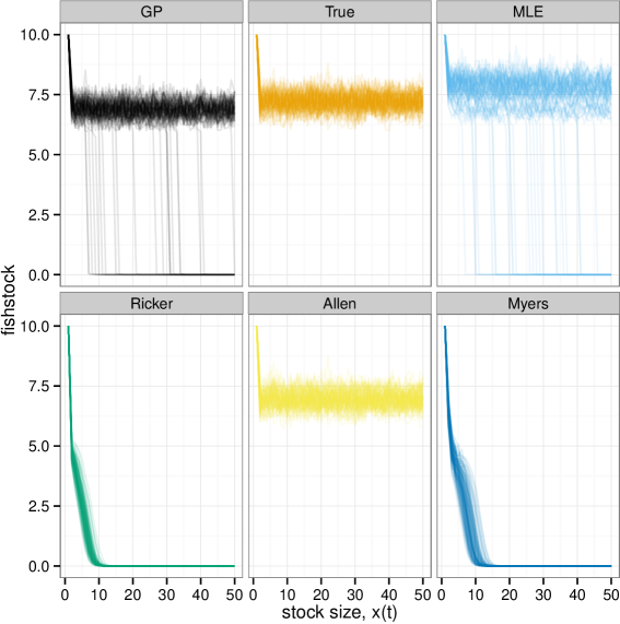
Figure 4: In the management context, GPDP outperforms approaches based on parametric models. We show 100 replicate simulations of the stock dynamics (Eqn 1) under the policies derived from each of the estimated models, as well as the policy based on the exact underlying model.

In Figure 4, we show the consequences of managing 100 replicate realizations of the simulated fishery under policies derived from each model. The structurally correct model under-harvests, leaving the stock to vary around its unfished optimum. The structurally incorrect Ricker model over-harvests the population past the tipping point consistently, resulting in the immediate crash of the stock and thus leads to minimal long-term catch.

The results across replicate stochastic simulations are most easily compared by using the relative differences in net present value realized by each of the model (Figure 5). Although not perfect, the GPDP consistently realizes a value close to the optimal solution, and avoids ever driving the system across the tipping point, which results in the near-zero value cases in the parametric models.

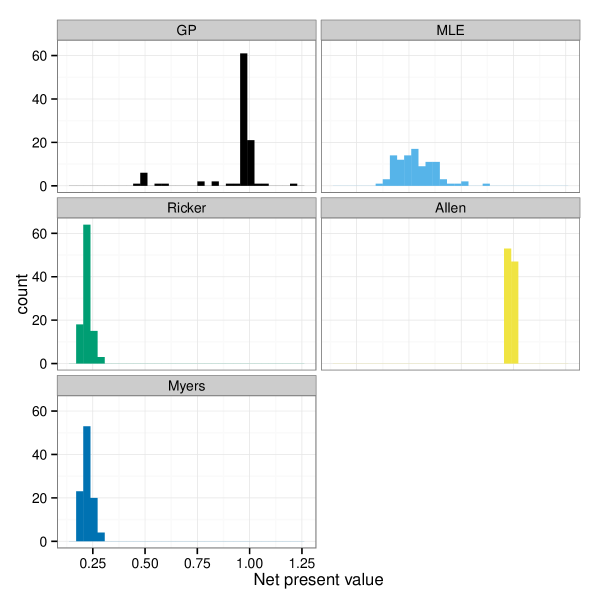
Figure 5: Histograms of the realized net present value of the fishery over a range of simulated data and resulting parameter estimates. For each data set, the three models are estimated as described above.

Sensitivity Analysis

These results are not sensitive to the modeling details of the simulation. The GPDP estimate remains very close to the optimal solution (obtained by knowing the true model) across changes to the training simulation, scale of stochasticity, parameters or structure of the underlying model. In the Supplement, we consider both a Latin hypercube approach and a more focused investigation of the effects of the relative distance to the Allee threshold and the variance of process stochasticity.

The GPDP is only weakly influenced by increasing stochasticity or increasing Allee effects over much of the range (Figure S2). Larger $\sigma$ or higher Allee levels make even the optimal solution without any model or parameter uncertainty unable to harvest the population effectively (e.g. the stochasticity is large enough to violate the self-sustaining criterion of Reed (1979)).

Discussion

Simple, mechanistically motivated models offer the potential to increase our basic understanding of ecological processes (Geritz and Kisdi 2012, Cuddington et al. 2013). But such models can be both inaccurate and misleading when used in a decision making framework. In this paper we tackled two aspects of uncertainty that are common to many ecological decision-making problems and fundamentally challenging to existing approaches that largely rely on parametric models:

1. We do not know the correct models for ecological systems.

2. We have limited data from which to estimate the model.

We have illustrated how the use of non-parametric methods provides more reliable solutions in the sequential decision-making problem.

Traditional model-choice approaches can be positively misleading

Our results illustrate that model-choice approaches can be absolutely misleading – by providing support to models that cannot capture tipping point dynamics because they have fewer parameters and the data are far from the tipping point. That is, when the data come from around the stable steady state, all the parametric models are approximately linear and approximately identical. Thus, it is intuitive that all model selection methods choose the simplest model. In a complex world, the result is suboptimal. But in a world that might contain tipping points, the result could be disastrous.

Many managers both in fisheries and beyond face a similar situation: they have not observed the population dynamics at all possible densities. A lack of comprehensive data at all population sizes, combined with the inability to formulate accurate population models for low population sizes in the absence of data, makes this situation the rule more than the exception. Relying on parametric models and model choice processes that favor simplicity ignores this basic reality. For a long time, Carl Walters (e.g. Walters and Hilborn 1978) has argued that if we began by fishing any newly exploited population down to very low levels and then let it recover, we would be much better at estimating population dynamics and thus predicting the optimal harvest levels. While certainly true, this presents a rather risky policy in the face of potential tipping points. The GPDP offers a risk-adverse alternative.

GPDP population dynamics capture larger uncertainty in regions where the data are poor

Parametric models perform most poorly when we seek a management strategy outside the range of the observed data. The GPDP, in contrast, leads to a predictive model that expresses a great deal of uncertainty about the probable dynamics outside the range of the observed data, while retaining very good predictive accuracy inside the range. The management policy based on by the GPDP balances uncertainty outside the range of the observed data against the immediate value of the harvest, and acts to stabilize the population dynamics in a region of state space in which the predictions are reliably reflected by the data.

Such problems are ubiquitous across ecological decision-making and conservation where the greatest concerns involve decisions that lead to population sizes that have never been observed and for which we do not know the response – whether this is the collapse of a fishery, the spread of an invasive, or the loss of habitat.

The role of the prior

Outside of the observed range of the data, the GP reverts to the prior, and consequently the choice of the prior can also play a significant role in determining the optimal policy. In the examples shown here we have selected a prior that is both relatively uninformative (due to the broad priors placed on its parameters $\ell$ and $\sigma$ and simple (the choice of our covariance function, Eqns 12 and 13 ). In practice, these should be chosen to confer particular biological properties. In principle, this may allow a manager to improve the performance of the GPDP by adding detail as is justified. For instance, it would be possible to use a linear or a Ricker-shaped mean in the prior without making the much stronger assumption that the Ricker is the structurally correct model (Sugeno and Munch 2013a). One fruitful avenue of future research is identifying criteria to ensure the prior and the reward function are chosen appropriately for the problem at hand.

Appendix A Code

All code used in producing this analysis has been embedded into the manuscript sourcefile using the Dynamic Documentation tool, knitr for the R language (Xie 2013), available at github.com/cboettig/nonparametric-bayes/

To help make the mathematical and computational approaches presented here more accessible, we provide a free and open source (MIT License) R package that implements the GPDP process as it is presented here. Users should note that at this time, the R package has been developed and tested explicitly for this analysis and is not yet intended as a general purpose tool. The manuscript source-code described above illustrates how these functions are used in this analysis. This package can be installed following the directions above.

Dependencies & Reproducibility

The code provided should run on any common platform (Windows, Mac or Linux) that has R and the necessary R packages installed (including support for the jags Gibbs sampler). The DESCRIPTION file of our R package, nonparametricbayes, lists all the software required to use these methods. Additional software requirements for the other comparisons shown here, such as the Gibbs sampling for the parametric models, are listed under the Suggested packages list.

Nonetheless, installing the dependencies needed is not a trivial task, and may become more difficult over time as software continues to evolve. To facilitate reuse, we also provide a Dockerfile and Docker image that can be used to replicate and explore the analyses here by providing a copy of the computational environment we have used, with all software installed. Docker sofware (see docker.com) runs on most platforms as well as cloud servers. Use the command:

docker run -dP cboettig/nonparametric-bayes

to launch an RStudio instance with the necessary software already installed. See the Rocker-org project, github.com/rocker-org for more detailed documentation on using Docker with R.

Appendix B Data

Dryad Data Archive

While the data can be regenerated using the code provided, for convenience CSV files of the data shown in each graph are made available on Dryad, along with the source .Rmd files for the manuscript and supplement that document them.

Training data description

Each of our models $f(S_{t})$ must be estimated from training data, which we simulate from the Allen model with parameters $r=$ 2, $K=$ 8, $C=$ 5, and $\sigma_{g}=$ 0.05 for $T=$ 40 timesteps, starting at initial condition $X_{0}=$ 5.5. The training data can be seen in Figure 1 and found in the table figure1.csv.

Training data for sensitivity analyses

A further 96 unique randomly generated training data sets are generated for the sensitivity analysis, as described in the main text. The code provided replicates the generation of these sets.

Appendix C Model performance outside the predicted range (Fig S1)

Figure S1 illustrates the performance of the GP and parametric models outside the observed training data. The mean trajectory under the underlying model is shown by the black dots, while the corresponding prediction made by the model shown by the box and whiskers plots. Predictions are based on the true expected value in the previous time step. Predicted distributions that lie entirely above the expected dynamics indicate the expectation of stock sizes higher than what is actually expected. The models differ both in their expectations and their uncertainty (colored bands show two standard deviations away). Note that the GP is particularly uncertain about the dynamics relative to structurally incorrect models like the Ricker.

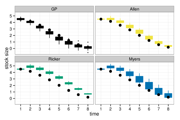
Figure S1: Outside the range of the training data (Figure 1), the true dynamics (black dots) fall outside the uncertainty (two standard deviations, colored bands) of the structurally incorrect parametric models (Ricker, Myers), but inside the uncertainty predicted by the GP. Points show the stock size simulated by the true model. Overlay shows the range of states predicted by each model, based on the state observed in the previous time step. The Ricker model always (wrongly) predicts positive population growth, while the actual population shrinks in each step as the initial condition falls below the Allee threshold of the underlying model (Allen). Note that because it does not assume a parametric form but instead relies more directly on the data, the GP is both more pessimistic and more uncertain about the future state than the parametric models.

Appendix D Further sensitivity analysis (Fig S2 - 3)

We perform 2 sensitivity analyses. The first focuses on illustrating the robustness of the approach to the two parameters that most influence stochastic transitions across the tipping point: the position of the Allee threshold and the scale of the noise (Fig S2).

Changing the intensity of the stochasticity or the distance between stable and unstable steady states does not impact the performance of the GP relative to the optimal solution obtained from the true model and true parameters. The parametric models are more sensitive to this difference. Large values of $\sigma$ relative to the distance between the stable and unstable point increases the chance of a stochastic transition below the tipping point. More precisely, if we let $L$ be the distance between the stable and unstable steady states, then the probability that fluctuations drive the population across the unstable steady state scales as

$\exp\left(\frac{L^{2}}{\sigma^{2}}\right)$

(see Gardiner (2009) or Mangel (2006) for the derivation).

Thus, the impact of using a model that underestimates the risk of harvesting beyond the critical point is considerable, since this such a situation occurs more often. Conversely, with large enough distance between the optimal escapement and unstable steady state relative to $\sigma$, the chance of a transition becomes vanishingly small and all models can be estimated near-optimally. Models that underestimate the cost incurred by population sizes fluctuating significantly below the optimal escapement level will not perform poorly as long as those fluctuations are sufficiently small. Fig S2 shows the net present value of managing under teh GPDP remains close to the optimal value (ratio of 1), despite varying across either noise level or the the position of the allee threshold.

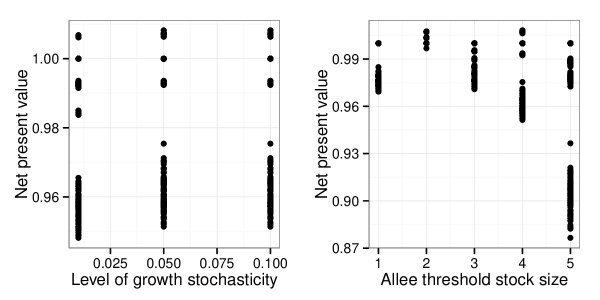
Figure S2: The effect of increasing noise or decreasing Allee threshold levels on the net present value of the fishery when managed under the GPDP, relative to managing under the true model (with known parameters). Other than the focal parameter (stochasticity, Allee threshold), other parameters are held fixed as above to illustrate this effect.

The Latin hypercube approach systematically varies all combinations of parameters, providing a more general test than varying only one parameter at a time. We loop across eight replicates of three different randomly generated parameter sets for each of two different generating models (Allen and Myers) over two different noise levels (0.01 and 0.05), for a total of 8 x 3 x 2 x 2 = 96 scenarios. The Gaussian Process performs nearly optimally in each case, relative to the optimal solution with no parameter or model uncertainty (Figure S10, appendix).

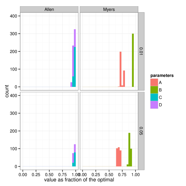
Figure S3: Sensitivity Analysis. Histograms shows the ratio of the realized net present value derived when managing under the GPDP over the optimal value given the true model and true parameters. Values of 1 indicate optimal performance. Columns indicate different models, rows different noise levels, and colors indicate the parameter set used. Grouped over stochastic replicates applying the contol policy and stochastic replicates of training data generated from the model indicated, see raw data for details. Randomly chosen parameter values for the models shown in tables below.

Table S1: Randomly chosen parameter sets for the Allen models in Figure S3.

	r	K	theta
set.A	1.103	7.949	2.288
set.B	1.485	9.775	3.524

Table S2: Randomly chosen parameter sets for the Myers models in Figure S3.

	r	K	C
set.C	1.769	10.46	4.301
set.D	2.075	10.95	4.915

Appendix E MCMC analyses

This section provides figures and tables showing the traces from each of the MCMC runs used to estimate the parameters of the models presented, along with the resulting posterior distributions for each parameter. Priors usually appear completely falt when shown against the posteriors, but are summarized by tables the parameters of their corresponding distributions for each case.

GP MCMC (Fig S4-5)

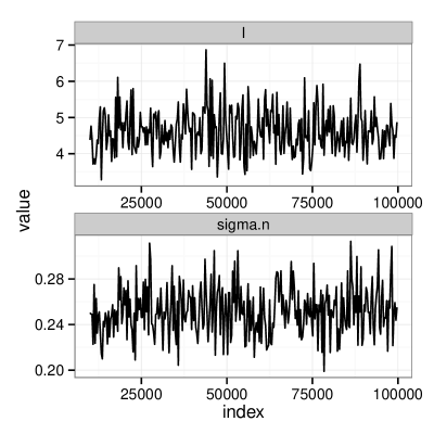
Figure S4: Traces from the MCMC estimates of the GP model show reasonable mixing (no trend) and sampling rejection rate (no piecewise jumps)

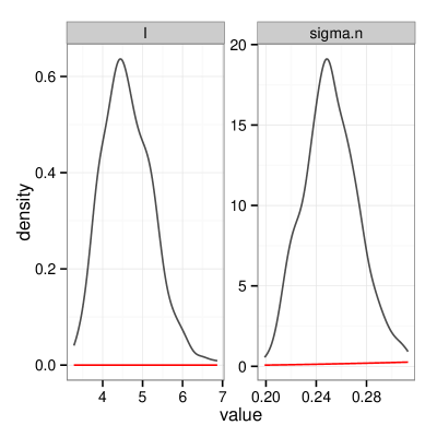
Figure S5: Posterior distributions from the MCMC estimate of the GP model. Prior curves shown in red; note the posterior distributions are significantly more peaked than the priors, showing that the data has been informative and is not driven by the priors.

Ricker Model MCMC (Fig S6-7)

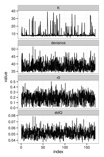
Figure S6: Traces from the MCMC estimates of the Ricker model show reasonable mixing (no trend) and sampling rejection rate (no piecewise jumps). stdQ refers to the estimate of $\sigma$; deviance is -2 times the log likelihood.

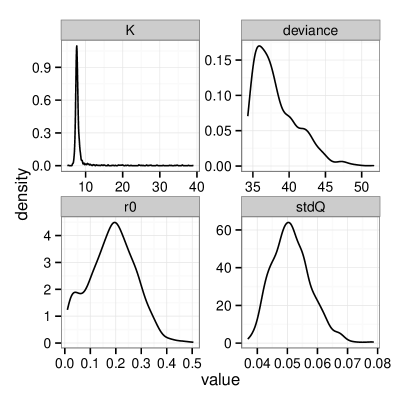
Figure S7: Posteriors from the MCMC estimate of the Ricker model. Note that the model estimates a carrying capacity $K$ very close to the true equilibrium where most of the observations were made, but is less certain about the growth rate.

Table S3: Parameterization range for the uniform priors in the Ricker model

parameter	lower.bound	upper.bound
$r$	0.01	20
$K$	0.01	40
$\sigma$	1e-06	100

Myers Model MCMC (Fig S8-9)

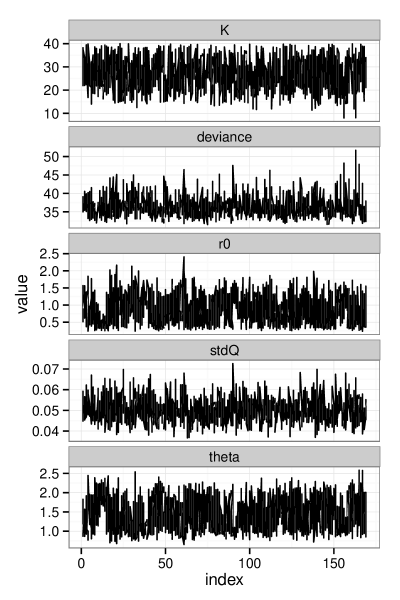
Figure S8: Traces from the MCMC estimates of the Myers model show reasonable mixing (no trend) and sampling rejection rate (no piecewise jumps). stdQ refers to the estimate of $\sigma$; deviance is -2 times the log likelihood.

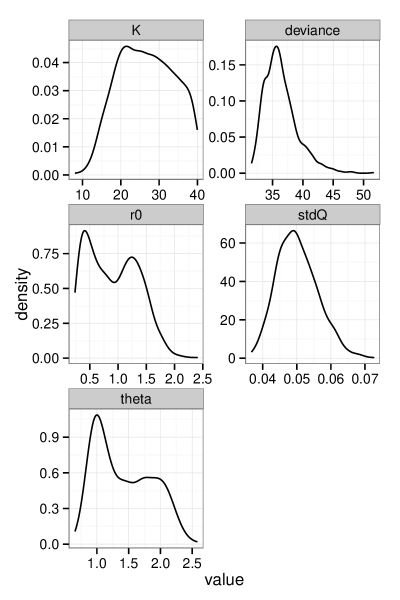
Figure S9: Posterior distributions from the MCMC estimates of the Myers model. Note that with more free parameters, the posteriors reflect greater uncertainty. In particular, the parameter $\theta$ includes values both above 2, resulting in a tipping point, and below 2, where no tipping point exists in the model. Though the dynamic program will integrate over the full distribution, including those values corresponding to tipping points, the weight of the model lies in the region without tipping points.

Table S4: Parameterization range for the uniform priors in the Myers model

parameter	lower.bound	upper.bound
$r$	1e-04	10
$K$	1e-04	40
$\theta$	1e-04	10
$\sigma$	1e-06	100

Allen Model MCMC (Fig S10-11)

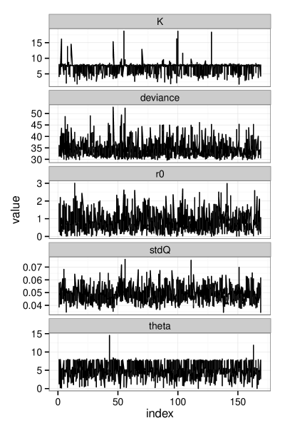
Figure S10: Traces from the MCMC estimates of the Allen model show reasonable mixing (no trend) and sampling rejection rate (no piecewise jumps). stdQ refers to the estimate of $\sigma$; deviance is -2 times the log likelihood.

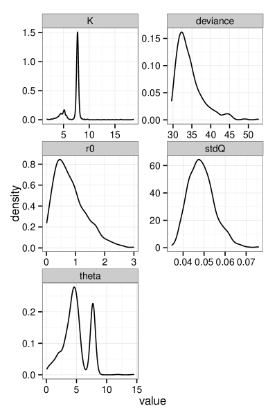
Figure S11: Posteriors from the MCMC estimate of the Allen model. The Allen model is the structurally correct model. Despite potential identfiability issues in distinguishing between the stable and unstable points ($K$ and $\theta$ respectively), the posterior estimates successfully reflect both the the upper stable point ($K$), as well as the significant probabilty of a tipping point ($\theta$) somewhere between $K$ and extinction (0).

Table S5: Parameterization range for the uniform priors in the Allen model

parameter	lower.bound	upper.bound
$r$	0.01	6
$K$	0.01	20
$X_{C}$	0.01	20
$\sigma$	1e-06	100

Gardiner, C. 2009. Stochastic Methods: A Handbook for the Natural and Social Sciences (Springer Series in Synergetics). Page 447. Springer.

Mangel, M. 2006. The Theoretical Biologist’s Toolbox: Quantitative Methods for Ecology and Evolutionary Biology. Cambridge University Press.

Xie, Y. 2013. Dynamic Documents with R and knitr. Chapman; Hall/CRCBoca Raton, Florida.