Exploring Sparsity in Multi-class Linear Discriminant Analysis

Abstract

Recent studies in the literature have paid much attention to the sparsity in linear classification tasks. One motivation of imposing sparsity assumption on the linear discriminant direction is to rule out the noninformative features, making hardly contribution to the classification problem. Most of those work were focused on the scenarios of binary classification, such as Fan et al. (2012), Cai and Liu (2011) and Mai et al. (2012). In the presence of multi-class data, preceding researches recommended individually pairwise sparse linear discriminant analysis(LDA), such as Cai and Liu (2011),Fan et al. (2012). However, further sparsity should be explored. In this paper, an estimator of grouped LASSO type is proposed to take advantage of sparsity for multi-class data. It enjoys appealing non-asymptotic properties which allows insignificant correlations among features. This estimator exhibits superior capability on both simulated and real data.

Keywords: Linear discriminant analysis, Multi-class, Sparsity

1 Introduction

Suppose that there is a collection of $i.i.d.$ random pairs $\{(X_{1},Y_{1}),\ldots,(X_{N},Y_{N})\}$. The vector $X_{j}\in\mathbb{R}^{p}$ contains measurements of $p$ features and the label $Y_{j}\in\{1,2,\ldots,K\}$ for $j=1,\ldots,N$. It is assumed that $P_{(X,Y)}(x,y)=P_{Y}(y)P_{X|Y}(x|y)$. The label $Y$ obeys an unknown distribution with $\mathbb{P}(Y=j)=\pi_{j},j=1,\ldots,K$ and $\sum_{j=1}^{K}\pi_{j}=1$. Given the sample data, the objective is to design a classifier:

$$\mathcal{C}:\mathbb{R}^{p}\to\{1,2,\ldots,K\},$$

such that $\mathbb{P}_{(X,Y)}(\{Y\neq\mathcal{C}(X)\})$ is minimized. In the simplest form, $\mathcal{C}(\cdot)$ is favored to comprise strategies based on linear functions, which is widely known as linear discriminant analysis(LDA). The LDA model assumed that the conditional distributions $X|Y=k,k=1,\ldots,K$ are Gaussian and they are

$$X|Y=k\sim\mathcal{N}(\mu_{K},\Sigma),\quad k=1,2,\ldots,K.$$

It is worth noting that the assumptions of Gaussian distributions can be relaxed to elliptical distributions, see Cai and Liu (2011). Denote $n_{k}:=\sharp\{j:Y_{j}=k,j=1,\ldots,N\}$ for $k=1,\ldots,K$ with $\sum_{j=1}^{K}n_{j}=N$. LDA performs pairwise classification via taking a linear combination of features as the criterion. More exactly, to distinguish between class $l$ and $k$ for $1\leq l\neq k\leq K$, LDA produces the following classifier:

$$\phi_{k,l}(x):=\begin{cases}k,&\text{if }(x-(\mu_{k}+\mu_{l})/2)^{\prime}\Sigma^{-1}\delta_{k,l}+\log(\pi_{k}/\pi_{l})>0\\ l,&\text{otherwise}\end{cases}$$ (1)

, where $\delta_{k,l}:=\mu_{k}-\mu_{l}$. It is famous that $\phi_{k,l}(x)$ is the perfect classifier which requires prerequisite knowledge of $\Sigma,\mu_{l},\mu_{k},\pi_{l},\pi_{k}$. In practice, we construct a classifier $\hat{\phi}_{k,l}(x)$ which mimics $\phi_{k,l}(x)$ by plugging corresponding estimators: $\hat{\Sigma},\hat{\mu}_{k},\hat{\mu}_{l},\hat{\pi}_{k},\hat{\pi}_{l}$ into (1). We know that in the binary case $\mathbb{P}_{(X,Y)}(\{Y\neq\hat{\phi}_{k,l}(X)\})\to\mathbb{P}_{(X,Y)}(\{Y\neq\phi_{k,l}(X)\})$ in probability when $p$ is frozen and $\hat{\Sigma},\hat{\mu}$ are chosen as the sample covariance and sample mean respectively, see Anderson (2003). However, as proved in Bickel and Levina (2004), $\hat{\phi}_{k,l}(x)$ in this mode performs poorly in the case $p\gg N$ which now arises conventionally in various applications. It turns out to be tricky to construct a stable estimator of $\Sigma^{-1}$ when $p\gg N$ . Sparsity assumptions have henceforth been proposed, such as Fan et al. (2012), Fan and Fan (2008), Mai et al. (2012) and Shao et al. (2011). There are two directions for the motivations of raising sparsity assumptions. One is that the sparsity assumption on $\Sigma$ or $\Sigma^{-1}$ enables us to propose advantageous estimators through convex optimization, such as Yuan (2010) and Cai et al. (2012). The other direction is to impose sparsity assumptions directly on the Bayes direction $\beta_{k,l}=\Sigma^{-1}\delta_{k,l}$, see Cai and Liu (2011) and Mai et al. (2012). It corresponds to the situation that merely a small portion of the features is relevant to the classification problem, which leads to a favorable interpretation. Actually, the sparsity on $\Sigma^{-1}$ and $\delta_{k,l}$ indicates the sparsity of $\beta_{k,l}$. In this paper, the Bayes directions: $\beta_{k,l}$ are presumed to be sparse for $1\leq k\neq l\leq K$.
We begin by introducing the notations and definitions. Let $\mathcal{Y}:=\{Y_{1},Y_{2},\ldots,Y_{N}\}$. Define the set

$$\mathcal{S}_{+}^{p}:=\{A\in\mathbb{R}^{p\times p}:A=A^{\prime},A\succeq 0\}.$$

We denote by $T_{k,l}$ the support of $\beta_{k,l}$ and by $s_{k,l}$ the cardinality of $T_{k,l}$ for $1\leq k\neq l\leq K$. Let $\hat{\mu}_{k}=n_{k}^{-1}\sum_{Y_{j}=k}X_{j}$ for $k=1,\ldots,K$ and

$$S=(N-K)^{-1}\sideset{}{{}_{k=1}^{K}}{\sum}\sideset{}{{}_{Y_{j}=k}}{\sum}(X_{j}-\hat{\mu}_{k})(X_{j}-\hat{\mu}_{k})^{\prime}.$$

Let $\hat{\delta}_{k,l}=\hat{\mu}_{k}-\hat{\mu}_{l}$. Meanwhile, suppose that $s=\text{card}(T)\ll p$ where $T=\bigcup\limits_{k=2}^{K}T_{1,k}$. To conduct pairwise discrimination, there is no need to estimate each $\beta_{k,l}$ for $1\leq k\neq l\leq K$ on account of $\beta_{k,l}=\beta_{1,l}-\beta_{1,k}$. Consequently, it is sufficient to estimate $\beta_{1,k}$ for $k=2,\ldots,K$. For the sake of brevity, define $\beta_{k}:=\beta_{1,k+1}$, $\delta_{k}=\delta_{1,k+1}$ for $k=1,\ldots,K^{\prime}$ with $K^{\prime}=K-1$. More exactly, suppose $\beta_{k}=(\beta_{k}^{1},\beta_{k}^{2},\ldots,\beta_{k}^{p})$ for $k=1,\ldots,K^{\prime}$. Given any $1\leq j\leq p$, define $\beta^{j}=:(\beta_{1}^{j},\ldots,\beta_{K^{\prime}}^{j})$, namely by stacking all the $j$-th entry of $\beta_{k},1\leq k\leq K^{\prime}$ into one vector. The vector $\beta^{j}$ is associated with the role of the $j$-th feature in the classification problem. Define $\Delta_{k}=\left<\Sigma^{-1}\delta_{k},\delta_{k}\right>$ for $1\leq k\leq K^{\prime}$ and $\Delta=\sum_{k=1}^{K^{\prime}}\Delta_{k}$. For any matrix $A\in\mathcal{S}_{+}^{p}$, we adopt the following notations: $A_{\min}^{+}=\min_{1\leq j\leq p}A_{jj}$, $A_{\max}^{+}=\max_{1\leq j\leq p}A_{jj}$ and $A^{-}_{\max}=\max_{1\leq i\neq j\leq p}|A_{ij}|$. Let $A_{T,:}$ and $A_{:,T}$ denote the submatrix of $A$ with corresponding rows and columns. Denote $\delta^{T}$ the subvector of $\delta$ with entries indexed by $T$. Let $T^{c}$ denote the complement of $T$. For any $v\in\mathbb{R}^{p}$, let $\|v\|$ be the usual $l_{2}$ norm and $|v|_{\infty}=\max_{1\leq i\leq p}|v_{i}|$. We also define $(x)_{+}:=x\mathbb{I}(x\geq 0)$ as the truncation function where $\mathbb{I}(\cdot)$ is the indicator function.
The following estimator was employed for sparse LDA when $K=2$ in Kolar and Liu (2013) and Fan et al. (2012).

$$\hat{\beta}_{1}:=\underset{\hat{\delta}_{1}^{\prime}\beta=1}{\arg\min}\quad\frac{1}{2}\beta^{\prime}S\beta+\lambda|\beta|_{1}$$ (2)

The $l_{1}$ norm penalty is aimed at promoting a sparse solution. A similar estimator is:

$$\hat{\beta}_{1}:=\underset{\beta\in\mathbb{R}^{p}}{\arg\min}\frac{1}{2}\beta^{\prime}S\beta-\hat{\delta}_{1}^{\prime}\beta+\lambda|\beta|_{1}.$$ (3)

The estimator (3) resembles the one proposed in Mai et al. (2012) which is of regression type. In contrast to these estimators of LASSO type, another estimator(LPD) which borrowed the idea of Dantzig selector was studied in Cai and Liu (2011):

$$\tilde{\beta}_{1}:=\underset{\beta\in\mathbb{R}^{p}}{\arg\min}\{|\beta|_{1}:|S\beta-\hat{\delta}_{1}|_{\infty}\leq\lambda\}$$ (4)

If $K\geq 3$, an immediate approach is to implement the above estimators for $\beta_{1},\beta_{2},\ldots,\beta_{K^{\prime}}$ separately. Its drawback resides in the ignorance of the multi-class information. One intention of imposing sparsity assumptions on $\beta_{k}$ derives from the objective of expelling the noninformative features displaying weak connections with the labels. It is unexceptional to expect that most the insignificant features will stay valueless when discriminating class $k$ and $l$ for different pairs $(k,l)$. There is where further sparsity might be explored. Intuitively, we hope that $\beta^{u}=0$ if the $u$-th feature is a nuisance feature. However, the individually pairwise sparse LDA is inferior to mis-include some nuisance features due to correlation and the insufficiency of data. Actually, our simulation result in Section 4 reflects that different noisy features might be mis-selected by pairwise estimation as (4). Chances of making this type of mistakes indeed can be decreased based on the same data when we take into account the grouped sparsity. To handle the grouped sparsity, we propose the following estimator:

$$(\hat{\beta}_{1},\ldots,\hat{\beta}_{K^{\prime}}):=\underset{\beta_{1},\ldots,\beta_{K^{\prime}}\in\mathbb{R}^{p}}{\arg\min}\sum\limits_{k=1}^{K^{\prime}}\frac{1}{2}\beta_{k}^{\prime}S\beta_{k}-\sum\limits_{k=1}^{K^{\prime}}\hat{\delta}_{k}^{\prime}\beta_{k}+\sum\limits_{j=1}^{p}\lambda_{j}||\beta^{j}||.$$ (5)

The regularization parameters $\lambda_{j},j=1,\ldots,p$ are positive and can be decided practically through cross-validation. Theoretic analysis will confirm that carefully selected $\lambda_{j},j=1,\ldots,p$ can yield attractive performances of (5). It is apparent that, when $K=2$ and $\lambda_{j}=\lambda,j=1,\ldots,p$, (5) is reduced to the commonly studied estimator (3). Meanwhile, it is easy to verify the convexity of the optimization problem in (5), which can be solved efficiently by many off-the-shelf algorithms. The estimator (5) is analogous to the LASSO estimator accommodated for problems either with grouped sparsity,Yuan and Lin (2006) or of multi-task regression, Lounici et al. (2009). We should point out that grouped sparsity for multi-class classification has been considered in Merchante et al. (2012) in a linear regression style combined with optimal scoring. Comparable methods can be also found in Zhu et al. (2014) which was used to classify Alzheimer’s disease. Variable selection for multi-class data has been studied experimentally in Lê Cao et al. (2011) based on partial least square discriminant analysis. People also studied the classification task for multi-labeled data in Han et al. (2010), in which case each $Y_{j}$ may have multiple entries. In addition, the paper by Witten and Tibshirani (2011) proposed a penalized Fisher discriminant method that can be extended to the multi-class situation, which, however, is non-convex and thereby is deficient in theoretic guarantees of its performance. After the completion of this paper, we noticed that Mai et al. (2014) proposed the same estimator as (5), where its theoretic properties were also studied. The analysis in our paper is completely different and our simulation results emphasized on the advantages of (5) over the individually pairwise classification.
The paper will be organized as follows. In section 2, some theoretic properties of the estimator will be presented. Then experimental results on both simulated and real data will be reported in Section 4, 5, in which we will compare the performance of (5) and (4), (3).

2 Theoretic properties

In this section, we turn to the theoretic properties of estimator (5). The upper bound of the estimation error $\|\hat{\beta}^{j}-\beta^{j}\|,j=1,\ldots,p$ will be provided as long as $\frac{\Sigma^{-}_{\max}}{\Sigma^{+}_{\min}}$ is small enough. It is well-known that $\hat{\mu}_{1},\ldots,\hat{\mu}_{K},S$ are mutually independent and $S=\frac{1}{N-K}ZZ^{\prime}$ where $Z\in\mathbb{R}^{p\times(N-K)}$, see (Muirhead, 2009, Theorem 3.1.2). Every column of $Z$ has distribution as $\mathcal{N}(0,\Sigma)$ and they are $i.i.d.$. Meanwhile, we can check that conditioned on $\mathcal{Y}$,

$$\hat{\delta}_{k}\sim\mathcal{N}(\delta_{k},\frac{n_{1}+n_{k+1}}{n_{1}n_{k+1}}\Sigma),\quad k=1,\ldots,K^{\prime}.$$ (6)

Lemma 1 uncovers the concentration of $n_{i},1\leq i\leq K$, which will be useful in the proof of our main theorem. Similar inequalities as in Proposition 2 appear regularly in researches of compressed sensing and low rank matrix completion, see Koltchinskii (2011).

Lemma 1

There exists an event $\mathcal{A}$ with $\mathbb{P}(\mathcal{A})\geq 1-2\sum\limits_{k=1}^{K}e^{-N\pi_{k}/16}$ such that on $\mathcal{A}$,

$$n_{k}\in\left[\frac{N\pi_{k}}{2},\frac{3N\pi_{k}}{2}\right],\quad 1\leq k\leq K.$$

Proposition 2

Let $\bar{\pi}=\max_{2\leq k\leq K}\sqrt{\frac{\pi_{1}+\pi_{k}}{\pi_{1}\pi_{k}}}$ and $(\hat{\beta}_{1},\ldots,\hat{\beta}_{K^{\prime}})$ be the solution of (5). Then for any $t>0$, there exists an event $\mathcal{B}_{t}$ with $\mathbb{P}(\mathcal{B}_{t})\geq\mathbb{P}(\mathcal{A})-Kpe^{-t}-\frac{2Kp}{\sqrt{\pi}t}e^{-t^{2}}$ such that on $\mathcal{B}_{t}$ we have

$$\sum\limits_{j=1}^{p}\lambda_{j}\|\hat{\beta}^{j}\|\leq\sum\limits_{j=1}^{p}\lambda_{j}\|\beta^{j}\|+C_{0}\sum\limits_{j=1}^{p}\|\hat{\beta}^{j}-\beta^{j}\|\sqrt{\frac{\bar{\pi}\Sigma_{jj}(\Delta\vee K)t}{N-K}},$$

where $C_{0}>0$ is a universal constant. Furthermore, if $\lambda_{j}=\lambda,j=1,\ldots,p$ with

$$\lambda=2C_{0}\sqrt{\frac{\bar{\pi}\Sigma_{\max}^{+}(\Delta\vee K)t}{N-K}},$$ (7)

then on event $\mathcal{B}_{t}$, we have

$$\sum\limits_{j\notin T}\|\hat{\beta}^{j}\|\leq 3\sum\limits_{j\in T}\|\hat{\beta}^{j}-\beta^{j}\|.$$

Moreover, if $\lambda_{j}=2C_{0}\sqrt{\frac{\bar{\pi}\Sigma_{jj}(\Delta\vee K)t}{N-K}},j=1,\ldots,p$ in Proposition 2, it leads to $\sum\limits_{j\notin T}\lambda_{j}\|\hat{\beta}^{j}\|\leq 3\sum\limits_{j\in T}\lambda_{j}\|\hat{\beta}^{j}-\beta^{j}\|$ on event $\mathcal{B}_{t}$. Let $\mathcal{D}$ denote the event: $\mathcal{D}:=\big{\{}\{S^{-}_{\max}\leq 2\Sigma^{-}_{\max}\}\cap\{S^{+}_{\min}\geq\frac{1}{2}\Sigma^{+}_{\min}\}\big{\}}$.

Proposition 3

Suppose that $\lambda_{j}=\lambda,j=1,\ldots,p$ with $\lambda$ chosen in (7). On the event $\mathcal{D}\cap\mathcal{B}_{t}$ for any $t>0$, we have

$$\Big{(}\frac{\Sigma^{+}_{\min}}{2}-32s\Sigma^{-}_{\max}\Big{)}\sum\limits_{j\in T}\|\hat{\beta}^{j}-\beta^{j}\|^{2}+\frac{\Sigma^{+}_{\min}}{2}\sum\limits_{j\notin T}\|\hat{\beta}^{j}\|^{2}\leq 12\lambda\sum\limits_{j\in T}\|\hat{\beta}^{j}-\beta^{j}\|.$$ (8)

Furthermore, if $\Sigma^{+}_{\min}\geq 128s\Sigma^{-}_{\max}$, we have on the event $\mathcal{D}\cap\mathcal{B}_{t}$,

$$\sum\limits_{j\in T}\|\hat{\beta}^{j}-\beta^{j}\|^{2}\leq\frac{C_{1}\lambda^{2}s}{(\Sigma^{+}_{\min})^{2}}$$ (9)

and

$$\sum\limits_{j\notin T}\|\hat{\beta}^{j}\|^{2}\leq\frac{C_{1}\lambda^{2}s}{2(\Sigma^{+}_{\min})^{2}}.$$ (10)

for some constant $C_{1}>0$.

Proposition 4

Let $\lambda_{j}=\lambda,j=1,\ldots,p$ with $\lambda$ chosen as $(\ref{prop1lambda})$. Meanwhile, suppose that $\Sigma^{+}_{\min}\geq 128s\Sigma^{-}_{\max}$. For any $t>0$, on the event $\mathcal{D}\cap\mathcal{B}_{t}$, we have

$$\sup\limits_{1\leq j\leq p}\|\hat{\beta}^{j}-\beta^{j}\|\leq\frac{C_{2}\lambda}{\Sigma^{+}_{\min}}=2C_{0}C_{2}\sqrt{\frac{\bar{\pi}\Sigma^{+}_{\max}(\Delta\vee K)t}{(\Sigma^{+}_{\min})^{2}(N-K)}},$$

where $C_{2}=4+\frac{\sqrt{C_{1}}}{8}$.

For any $\zeta>0$, we define a thresholding function $\phi_{\zeta}(\cdot):\mathbb{R}\to\mathbb{R}$ as

$$\phi_{\zeta}(x)=\begin{cases}x,&|x|\geq\zeta\\ 0,&|x|<\zeta.\end{cases}$$

When we apply the function $\phi_{\zeta}$ to a vector $\beta$, it means we apply $\phi_{\zeta}$ to each entry of $\beta$. Theorem 5 follows immediately from Proposition 4, Lemma 8 and the definition of $\phi_{\zeta}(\cdot)$, which provides a sufficient condition for the support recovery of our estimator. In the case that $\Sigma^{+}_{\min}\approx\Sigma^{+}_{\max}$, the lower bound on $\min_{j\in T_{k}}|\beta_{k}^{j}|$ is of the order $O(\sqrt{\frac{(\Delta\vee K)\log(p\vee N)}{N}})$, which is similar to the necessary lower bound on the non-trivial entries of $\beta$ for sign consistency of (2) when $K=2$, see Kolar and Liu (2013).

Theorem 5

Under the same conditions of Proposition 4 and suppose that there exists some constants $C_{3}>0$ which are large enough such that $N\geq K+C_{3}\big{(}\frac{\Sigma^{+}_{\max}}{\Sigma^{+}_{\min}}\big{)}^{2}s^{2}\log(p\vee N)$. Then we have, with probability at least $1-2\sum\limits_{j=1}^{K}e^{-N\pi_{K}/16}-\frac{2}{p\vee N}$

$$|\hat{\beta}_{k}-\beta_{k}|_{\infty}\leq 4C_{0}C_{2}\sqrt{\frac{\bar{\pi}\Sigma^{+}_{\max}(\Delta\vee K)\log(p\vee N)}{(\Sigma^{+}_{\min})^{2}(N-K)}}=:\zeta.$$

Furthermore, suppose that for any $1\leq k\leq K^{\prime}$, $\min_{j\in T_{k}}|\beta_{k}^{j}|>2\zeta$. Define $\hat{\hat{\beta}}_{k}=\phi_{\zeta}(\hat{\beta}_{k})$ for $1\leq k\leq K^{\prime}$, then we have

$$\textrm{Supp}(\hat{\hat{\beta}}_{k})=\textrm{Supp}(\beta_{k}),\quad 1\leq k\leq K^{\prime},$$

with the same probability.

In Theorem 6, a lower bound on the estimation error of $\beta$ is given by assuming that $T_{1},\ldots,T_{K^{\prime}}$ are known in advance. Under the circumstances, the ideal estimators would be $\bar{\beta}_{k}^{T_{k}}=S_{T_{k},T_{k}}^{-1}\hat{\delta}_{k}$ and $\bar{\beta}_{k}^{T_{k}^{c}}=0$ for $1\leq k\leq K^{\prime}$. We then calculate $\mathbb{E}\|\bar{\beta}^{j}-\beta^{j}\|,1\leq j\leq p$ which can be regarded as benchmarks for the estimation errors. It confirms the optimality(except the logarithmic term) of the bound in Proposition 4 for $j\in\bigcap_{k=1}^{K^{\prime}}T_{k}$ when $\Sigma^{+}_{\min}\approx\Sigma^{+}_{\max}$. It should be noted that under the conditions of Proposition 4, we have $\Sigma^{+}_{\min}\|\beta_{k}\|^{2}\leq 2\Delta_{k}$ for $1\leq k\leq K^{\prime}$.

Theorem 6

Suppose we have access to $T_{1},\ldots,T_{K^{\prime}}$ and $\bar{\beta}_{k}$ are defined as above for $1\leq k\leq K^{\prime}$. Let $\underline{\pi}=\min_{2\leq k\leq K}\sqrt{\frac{\pi_{1}+\pi_{k}}{\pi_{1}\pi_{k}}}$. For any $1\leq j\leq p$, define $\kappa_{j}=\min_{1\leq k\leq K}(\Sigma_{T_{k},T_{k}}^{-1})_{jj}$, $\bar{\Delta}_{j}:=\sum_{k=1,j\in T_{k}}^{K^{\prime}}\Delta_{k}$, $K_{j}:=\sharp\{1\leq k\leq K^{\prime}:j\in T_{k}\}$ and $\omega_{j}=\sum_{k=1,j\in T_{k}}^{K^{\prime}}|\beta_{k}^{j}|^{2}$, then

$$\mathbb{E}\|\bar{\beta}^{j}-\beta^{j}\|_{2}^{2}\geq\frac{1}{2}\Big{[}\frac{\bar{\Delta}_{j}\kappa_{j}}{N-K}+\frac{K_{j}\kappa_{j}\underline{\pi}}{N-K}+\frac{\omega_{j}}{N-K}\Big{]}.$$

3 Algorithm to solve (5)

In this section, we briefly discuss how to adapt one existing algorithm to solve the minimization problem in (5). Let

$$f(\beta_{1},\ldots,\beta_{K^{\prime}}):=\frac{1}{2}\sum\limits_{k=1}^{K^{\prime}}\beta_{k}^{\prime}S\beta_{k}-\sum\limits_{k=1}^{K^{\prime}}\hat{\delta}_{k}^{\prime}\beta_{k}.$$

We will utilize the scheme in Liu and Ye (2010). The method attempts to approximate $f(\beta_{1},\ldots,\beta_{K^{\prime}})$ by

$$Af_{(\tilde{\beta}_{1},\ldots,\tilde{\beta}_{K^{\prime}})}(\beta_{1},\ldots,\beta_{K})=f(\tilde{\beta}_{1},\ldots,\tilde{\beta}_{K^{\prime}})+\left<\tilde{\nabla}_{f},\beta-\tilde{\beta}\right>+\frac{L}{2}||\beta-\tilde{\beta}||^{2}.$$

The parameter $L>0$ controls the deviation of $\beta$ from $\tilde{\beta}$ and $\tilde{\nabla}_{f}$ denotes the gradient of $f$ at $(\tilde{\beta}_{1},\ldots,\tilde{\beta}_{K^{\prime}})$. Then the accelerated gradient algorithm is applied to the function $Af_{(\tilde{\beta}_{1},\ldots,\tilde{\beta}_{K^{\prime}})}(\beta_{1},\ldots,\beta_{K})+\sum\limits_{j=1}^{p}\lambda_{j}\|\beta^{j}\|$. It updates $(\tilde{\beta}_{1},\ldots,\tilde{\beta}_{K^{\prime}})$ and $(\hat{\beta}_{1},\ldots,\hat{\beta}_{K^{\prime}})$ alternatively. One of the key points of this algorithm is that the solution of the following optimization problem,

$$\hat{v}:=\underset{v\in\mathbb{R}^{K}}{\arg\min}\frac{1}{2}||v-x||^{2}+\lambda||v||$$

has a closed form as $\hat{v}:=\frac{(\|x\|-\lambda)_{+}}{\|x\|}x$. This algorithm inherits the $O(1/k^{2})$ convergence rate of the accelerated gradient method.

4 Numerical Simulations

In this section, we will compare the performance of (5) and (4) on simulated data. As stated in Cai and Liu (2011), (4) can be formulated into a linear programming(LP) problem. The built-in LP solver in MATLAB works efficiently when $p$ is not tremendous. Actually, we set $n_{1}=n_{2}=n_{3}=20$ and $p=200$. The purpose of this simulation is to demonstrate the power of our estimator in variable selection. The result reveals that by implementing sparse LDA individually from (4), some nuisance features are mis-selected into the model. This can be prevented by our estimator (5). It should be noted that $\Sigma$ and $\mu_{1},\mu_{2},\mu_{3}$ are chosen quite generally without much special design in the simulation. Let $\Sigma\in\mathcal{S}^{p}_{+}$ be

$$\Sigma(4,1:3)=(1/4,1/3,1/4),\quad\Sigma(5,1:3)=(1/5,-1/4,1/5),\quad\textrm{diag}(\Sigma)=1.$$

Then we set $\beta_{1}=(-2,3,1,0,\ldots,0)^{\top}\in\mathbb{R}^{p}$, $\beta_{2}=(1,-2,-1.2,0,\ldots,0)\in\mathbb{R}^{p}$ and $\mu_{1}=0$. The vectors $\mu_{2}$ and $\mu_{3}$ are determined in line with the facts that $\mu_{2}=\Sigma\beta_{1}$ and $\mu_{3}=\Sigma\beta_{2}$. Denote $\tilde{\beta}_{1}$ and $\tilde{\beta}_{2}$ the solutions obtained from the LPD estimators (4) independently. Figure 1 shows how the entries of $\tilde{\beta}_{1}$ and $\tilde{\beta}_{2}$ vary accordingly as $\lambda$ grows. The variable selection process of $\tilde{\beta}_{1}$ and $\tilde{\beta}_{2}$ indicates the weakness in estimating $\beta_{1}$ and $\beta_{2}$ separately, owing to the scarcity of data. Indeed, incorporating inessential features occurs frequently when $N$ is small enough compared with $p$.

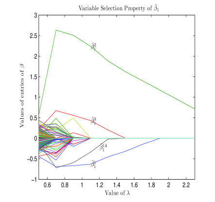
(a) Variable Selection property of $\tilde{\beta}_{1}$

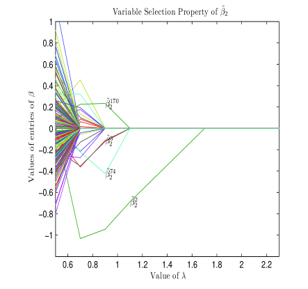
(b) Variable Selection property of $\tilde{\beta}_{2}$

Figure 1: Simulation $1$: Variable selection properties of $\tilde{\beta}_{1}$ and $\tilde{\beta}_{2}$ which are estimated individually via the LPD estimator when $\lambda$ is increasing. The non-vanished entries of $\tilde{\beta}_{1}$ and $\tilde{\beta}_{2}$ are depicted in the plots. The sample size $n_{1}=n_{2}=n_{3}=20$, which is much smaller than the number of features $p=200$. The result apparently attests that by estimating the Bayes’ directions separately, it is likely to mis-include the nuisance features into our model.

Then we switch to apply group sparsity in estimating $\beta_{1}$ and $\beta_{2}$ together. By choosing $\lambda_{1}=\ldots=\lambda_{p}=\lambda$, our estimator works as follows

$$(\hat{\beta}_{1},\hat{\beta}_{2}):=\underset{(\beta_{1},\beta_{2})\in(\mathbb{R}^{p},\mathbb{R}^{p})}{\arg\min}\frac{1}{2}\sum\limits_{k=1}^{2}\beta_{k}^{\prime}S\beta_{k}-\sum\limits_{k=1}^{2}\hat{\delta}_{k}^{\prime}\beta_{k}+\lambda\sum\limits_{j=1}^{p}||\beta^{j}||.$$

The variable selection property of $(\hat{\beta}_{1},\hat{\beta}_{2})$ is also examined as given in Figure 2. Compared with Figure 1, it is evident that the grouped sparse LDA works better in feature selection.

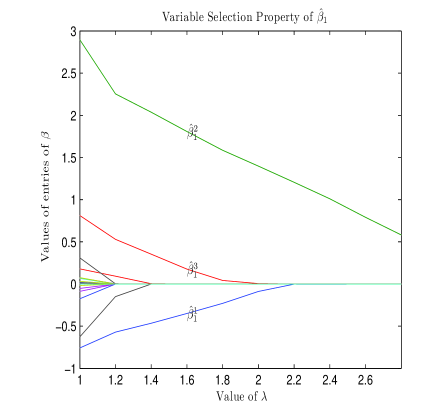
(a) Variable Selection property of $\hat{\beta}_{1}$

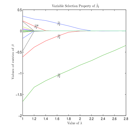
(b) Variable Selection property of $\hat{\beta}_{2}$

Figure 2: Simulation $1$: Variable selection properties of $(\hat{\beta}_{1},\hat{\beta}_{2})$ which are estimated through exploiting grouped sparsity with $\lambda$ growing. It confirms that both $\hat{\beta}_{1}$ and $\hat{\beta}_{2}$ are able to filter out the negligible features when $\lambda$ is attentively chosen.

In our second simulation, we consider more complex $\Sigma$ and $T_{1}\neq T_{2}$. In fact, $\Sigma$ is chosen as:

$$\Sigma_{i,j}=\frac{1}{3^{|i-j|}},\quad\text{for }1\leq i,j\leq p/2\quad\textrm{and}\quad\textrm{diag}(\Sigma)=1$$

Therefore, the correlations exist exclusively within the first $p/2$ features and the remaining ones are pure noise. Let $\beta_{1}=(-1.5,1,0,2,0,\ldots,0)^{\top}\in\mathbb{R}^{p}$, $\beta_{2}=(1,-1.8,-2,0,\ldots,0)^{\top}\in\mathbb{R}^{p}$ and $\mu_{1}=0$. Clearly, $\beta_{1}$ and $\beta_{2}$ have different supports. We sampled $n_{1}=n_{2}=n_{3}=20$ data points. Since $T_{1}\neq T_{2}$, it is not likely that the grouped sparsity estimator can identify the features correctly for both $\hat{\beta}_{1}$ and $\hat{\beta}_{2}$. For this reason, there is no obvious evidence of advantages for either (5) or (4) in the same sense of feature selection as in the former simulation. Instead, we inspect the $l_{2}$ magnitude of Bayes directions for each feature, $i.e.$, the values of $||\tilde{\beta}^{j}||$ and $||\hat{\beta}^{j}||$ for $j=1,\ldots,p$. The outcome is presented in Figure 3.

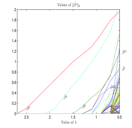
(a) Values of $\|\tilde{\beta}^{j}\|_{2}$

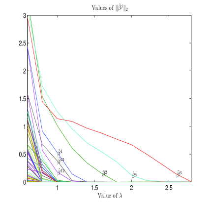
(b) Values of $\|\hat{\beta}^{j}\|_{2}$

Figure 3: Simulation $2$: values of $\|\hat{\beta}^{j}\|_{2}$ and $\|\tilde{\beta}^{j}\|_{2}$ for $j=1,\ldots,p$. In sub-Figure 3(a), it shows that the estimators $(\tilde{\beta}_{1},\tilde{\beta}_{2})$ places the irrelative features $12$ and $21$ in front of the relative feature $1$ as being more important. On the contrary, the grouped sparsity estimator $(\hat{\beta}_{1},\hat{\beta}_{2})$ produces the desired performance. The result in sub-Figure 3(b) entails that the four most informative features are actually $T_{1}\cup T_{2}$.

5 Experiments on real datasets

In this section, we will implement our estimators on several datasets. Our experiment is conducted on three datasets: GLIOMA dataset, MLL dataset, SRBCT dataset. These pre-processed datasets are available from Yang et al. (2006). In the GLIOMA dataset, there are $4434$ genes features chosen from $12625$ features with largest absolute values of $t$-statistics. The dataset contains $50$ samples in four classes with $n_{1}=14,n_{2}=7,n_{3}=14,n_{4}=15$. We split the data into a training set and a testing set. The training set contains $11,5,11,12$ samples from the four classes respectively. The remaining samples are treated as testing data. The MLL dataset includes $72$ samples from three classes with $5848$ features. The authors of Yang et al. (2006) already split the datasets into a training set and testing set. Therefore, we directly adopt our estimator to the training data. In the training set, $n_{1}=20,n_{2}=17,n_{3}=20$. In the testing set, it provides $4,3,8$ samples for each classes. In the SRBCT dataset, there are $83$ samples from four classes. The number of gene features is $2308$. The number of samples for each class is $n_{1}=29,n_{2}=11,n_{3}=18,n_{4}=25$. We also split the dataset into a training set and a testing set. In the training set, there are $26,9,16,22$ samples for each class.
To run LDA, $(\hat{\beta}_{1},\hat{\beta}_{2},\hat{\beta}_{3})$ or $(\hat{\beta}_{1},\hat{\beta}_{2})$ will be estimated from the training set and be employed to predict the labels of the testing data. Define $\hat{\pi}_{j}=\frac{n_{j}}{N}$ as the estimator of $\pi_{j},j=1,2,3$ where $n_{j}$ is based on the training set. The performance is certainly measured by the predicting error rate on the testing set. To demonstrate the efficiency of our estimator, we will compare our grouped LASSO estimator to the estimator (3). The regularization parameter $\lambda$ is chosen by $5$-folded cross validation on the training data. In the case that the error rates happen to be equal for different $\lambda$, we choose the largest one. The exactly same approaches will be applied to (5) and (3). The misclassification error rates are reported in Table 1, which shows that (5) and (3) have matching performance on SRBCT and MLL datasets. However, our grouped LASSO estimator (5) outperforms all the other estimators on GLIOMA dataset.

Estimator	GLIOMA	SRBCT	MLL
$\hat{\beta}$	0.00	0.00	0.00
	(0.15)	(0.00)	(0.00)
$\tilde{\beta}$	0.18	0.00	0.00
	(0.12)	(0.00)	(0.00)
Naive Bayes	0.64	0.90	0.53
$\tilde{\beta}:=S^{+}\hat{\mu}$	0.09	0.60	0.07

Table 1: Experiments on Real Datasets: $\hat{\beta}$ denotes our estimator of grouped LASSO type and $\tilde{\beta}$ denotes the estimator (3). The regularization parameter $\lambda$ is concluded by $5$-folded cross validation. After selecting the best value of $\lambda$, the error rates are reported based on the testing data and the standard variances are also reported in the parentheses, measured in $5$-folded cross validation on training data. In comparison, the performance of Naive Bayes classifier is also given for all the three datasets. Another trivial estimator is constructed via the pseudo-inverse of $S$.

6 Proofs

We begin by stating and proving two preliminary lemmas. Lemma 7 is related to the concentration of $S\beta_{k}-\hat{\delta}_{k}$ for $1\leq k\leq K^{\prime}$, while Lemma 8 will show that event $\mathcal{D}$ holds with high probability. The vectors $e_{1},\ldots,e_{p}$ represent the standard basis vectors in $\mathbb{R}^{p}$.

Lemma 7

For $1\leq k\leq K^{\prime}$, $1\leq j\leq p$ and any $t>0$, then conditioned on $\mathcal{A}$, we have with probability at least $1-\frac{2}{\sqrt{\pi}t}e^{-t^{2}}-e^{-t}$,

$$\big{|}e_{j}^{\prime}S\beta_{k}-e_{j}^{\prime}\hat{\delta}_{k}\big{|}\leq C_{0}\Big{[}\sqrt{\frac{\Sigma_{jj}\Delta_{k}t}{N-K}}\bigvee\frac{\sqrt{\Sigma_{jj}\Delta_{k}}t}{N-K}\bigvee\sqrt{\frac{24(\pi_{1}+\pi_{k+1})\Sigma_{jj}t}{N\pi_{1}\pi_{k+1}}}\Big{]}$$

Proof  We know that $|e_{j}^{\prime}S\beta_{k}-e_{j}^{\prime}\hat{\delta}_{k}|\leq|e_{j}^{\prime}S\beta_{k}-e_{j}^{\prime}\Sigma\beta_{k}|+|e_{j}^{\prime}\delta_{k}-e_{j}^{\prime}\hat{\delta}_{k}|$, thanks to the fact that $\delta_{k}=\Sigma\beta_{k}$. Based on (6), we get,

$$e_{j}^{\prime}\hat{\delta}_{k}|\mathcal{Y}\sim\mathcal{N}\Big{(}e_{j}^{\prime}\delta_{k},\frac{(n_{1}+n_{k+1})\Sigma_{jj}}{n_{1}n_{k+1}}\Big{)}.$$

By the concentration of Gaussian random variable, we have for any $t>0$,

$$\mathcal{P}\Big{(}|e_{j}^{\prime}\hat{\delta}_{k}-e_{j}^{\prime}\delta_{k}|\geq\sqrt{\frac{24(\pi_{1}+\pi_{k+1})\Sigma_{jj}t}{N\pi_{1}\pi_{k+1}}}\Big{|}\mathcal{A}\Big{)}\leq\frac{2}{\sqrt{\pi}t}e^{-t^{2}},$$

where the event $\mathcal{A}$ is defined in Lemma 1. Now we seek to bound $|e_{j}^{\prime}S\beta_{k}-e_{j}^{\prime}\Sigma\beta_{k}|$. Define

$$U=e_{j}^{\prime}S\beta_{k}-e_{j}^{\prime}\Sigma\beta_{k}=\frac{1}{N-K}\sum\limits_{i=1}^{N-K}(e_{j}^{\prime}Z_{:,i}Z_{:,i}^{\prime}\beta_{k}-e_{j}^{\prime}\Sigma\beta_{k})=\frac{1}{N-K}\sum\limits_{i=1}^{N-K}U_{i},$$

where $U_{i}=e_{j}^{\prime}Z_{:,i}Z_{:,i}^{\prime}\beta_{k}-e_{j}^{\prime}\Sigma\beta_{k}$ for $1\leq i\leq N-K$. Then we see that $\mathbb{E}U_{i}=0$ and $U_{1},\ldots,U_{N-K}$ are $i.i.d.$ sub-exponential random variable. Meanwhile,

$$\mathbb{E}U_{i}^{2}\leq\mathbb{E}(e_{j}^{\prime}Z_{:,i}Z_{:,i}^{\prime}\beta_{k})^{2}\leq\sqrt{\mathbb{E}(e_{j}^{\prime}Z_{:,i})^{4}\mathbb{E}(Z_{:,i}^{\prime}\beta_{k})^{4}}\leq C_{0}^{\prime}\Sigma_{jj}\Delta_{k}$$

By Bernstein inequality for the sum of independent sub-exponential random variable, such as (Vershynin, 2010, Corollary 5.17) we get

$$\mathbb{P}\Big{(}U\geq C_{0}\sqrt{\Sigma_{jj}\Delta_{k}}\big{[}\sqrt{\frac{t}{N-K}}\vee\frac{t}{N-K}\big{]}\Big{)}\leq e^{-t}$$

for some constant $C_{0}>0$.  

Lemma 8

Suppose that

$$N\geq K+C_{3}\Big{[}\Big{(}\frac{\Sigma^{+}_{\max}}{\Sigma^{-}_{\max}}\Big{)}^{2}\vee\Big{(}\frac{\Sigma^{+}_{\max}}{\Sigma^{+}_{\min}}\Big{)}^{2}\Big{]}\log(p\vee N)$$

for some constant $C_{3}>0$, there exists an event $\mathcal{D}$ with $\mathbb{P}(\mathcal{D})\geq 1-\frac{1}{p\vee N}$ such that on $\mathcal{D}$,

$$S^{+}_{\min}\geq\frac{\Sigma^{+}_{\min}}{2}\quad\textrm{and}\quad S^{-}_{\max}\leq 2\Sigma^{-}_{\max}$$

Proof  For any $1\leq j\leq p$, consider $S_{jj}-\Sigma_{jj}=\frac{1}{N-K}\sum_{i=1}^{N-K}\xi_{i}^{2}-\Sigma_{jj}$ with $\xi_{i}\sim\mathcal{N}(0,\Sigma_{jj})$ being independent for $1\leq i\leq N-K$. Akin to the proof of Lemma 7, we have with probability at least $1-e^{-t}$ for any $t>0$,

$$|S_{jj}-\Sigma_{jj}|\leq C_{3}^{\prime}\Sigma_{jj}\Big{[}\sqrt{\frac{t}{N-K}}\bigvee\frac{t}{N-K}\Big{]}.$$

Similarly we can get for $1\leq i\neq j\leq p$,

$$\mathbb{P}\Big{(}\big{|}S_{ij}-\Sigma_{ij}\big{|}\geq C_{3}^{\prime}\sqrt{\Sigma_{ii}\Sigma_{jj}}\Big{[}\sqrt{\frac{t}{N-K}}\bigvee\frac{t}{N-K}\Big{]}\Big{)}\leq e^{-t}.$$

The proof is completed after $t$ is adjusted to be $c_{3}^{\prime}\log(p\vee N)$ for some constant $c_{3}^{\prime}>0$.  

Proof of Lemma 1 Let $\epsilon_{1},\ldots,\epsilon_{n}$ be $i.i.d.$ Bernoulli random variable with $\mathbb{E}\epsilon_{1}=\pi$. The Hoeffding inequality states that, for any $0<\delta\leq\frac{1}{2}$,

$$\mathbb{P}\Big{(}\sum\limits_{j=1}^{n}\epsilon_{j}\geq n(1+\delta)\pi\Big{)}\leq e^{-\frac{n\delta^{2}\pi}{4}}$$

and

$$\mathbb{P}\Big{(}\sum\limits_{j=1}^{n}\epsilon_{j}\leq n(1-\delta)\pi\Big{)}\leq e^{-\frac{n\delta^{2}\pi}{4}}.$$

Lemma 1 follows immediately by applying Hoeffding inequality.  

Proof of Proposition 2 By the definition of $(\hat{\beta}_{1},\ldots,\hat{\beta}_{K^{\prime}})$, we have

$$\begin{split}\frac{1}{2}\sum\limits_{k=1}^{K^{\prime}}&\hat{\beta}_{k}^{\prime}S\hat{\beta}_{k}-\sum\limits_{k=1}^{K^{\prime}}\hat{\delta}_{k}^{\prime}\hat{\beta}_{k}+\sum\limits_{j=1}^{p}\|\hat{\beta}^{j}\|\\ \leq&\frac{1}{2}\sum\limits_{k=1}^{K^{\prime}}\beta_{k}^{\prime}S\beta_{k}-\sum\limits_{k=1}^{K^{\prime}}\hat{\delta}_{k}^{\prime}\beta_{k}+\sum\limits_{j=1}^{p}\|\beta^{j}\|.\end{split}$$

Denote $\Phi_{\beta}=[\beta_{1},\beta_{2},\ldots,\beta_{K^{\prime}}]\in\mathbb{R}^{p\times K^{\prime}}$ by arranging $\beta_{j},j=1,\ldots,K^{\prime}$ as columns. Simple algebras will lead to

$$\begin{split}\sum\limits_{j=1}^{p}\lambda_{j}&\|\hat{\beta}^{j}\|\leq-\frac{1}{2}\sum\limits_{k=1}^{K^{\prime}}(\hat{\beta}_{k}-\beta_{k})^{\prime}S(\hat{\beta}_{k}-\beta_{k})\\ +&\sum\limits_{j=1}^{p}\lambda_{j}\|\beta^{j}\|+\sum\limits_{j=1}^{p}(e_{j}^{\prime}S\Phi_{\beta}-(\hat{\delta}^{j})^{\prime})(\hat{\beta}^{j}-\beta^{j})\\ \leq&\sum\limits_{j=1}^{p}\lambda_{j}\|\beta^{j}\|+\sum\limits_{j=1}^{p}\|e_{j}^{\prime}S\Phi_{\beta}-(\hat{\delta}^{j})^{\prime}\|\|\hat{\beta}^{j}-\beta^{j}\|\end{split}$$ (11)

Then by Lemma 7, for any $1\leq k\leq K^{\prime}$, we have, conditioned on $\mathcal{A}$, with probability at least $1-\frac{2}{\sqrt{\pi}t}e^{-t^{2}}-e^{-t}$,

$$|e_{j}^{\prime}S\beta_{k}-\hat{\delta}_{k}^{j}|\leq C_{0}\sqrt{\frac{\bar{\pi}(\Delta_{k}\vee 1)\Sigma_{jj}t}{N-K}}.$$

Therefore, with probability at least $\mathbb{P}(\mathcal{A})-\frac{2Kp}{\sqrt{\pi}t}e^{-t^{2}}-Kpe^{-t}$, we have for all $j=1,\ldots,p$,

$$\|e_{j}^{\prime}S\Phi_{\beta}-(\hat{\delta}^{j})^{\prime}\|\leq C_{0}\sqrt{\frac{\bar{\pi}(\Delta\vee K)\Sigma_{jj}t}{N-K}}.$$

The proof is completed when we plug it into (11). When $\lambda_{j},j=1,\ldots,p$ are chosen as (7), we have

$$2\sum\limits_{j=1}^{p}\|\hat{\beta}^{j}\|\leq 2\sum\limits_{j=1}^{p}\|\beta^{j}\|+\sum\limits_{j=1}^{p}\|\hat{\beta}^{j}-\beta^{j}\|.$$

By the fact $\beta^{j}=0$ for any $j\notin T$, we get

$$2\sum\limits_{j\in T}\|\hat{\beta}^{j}\|+2\sum\limits_{j\notin T}\|\hat{\beta}^{j}\|\leq 2\sum\limits_{j\in T}\|\beta^{j}\|+\sum\limits_{j\in T}\|\hat{\beta}^{j}-\beta^{j}\|+\sum\limits_{j\notin T}\|\hat{\beta}^{j}\|.$$

Then we get $\sum_{j\notin T}\|\hat{\beta}^{j}\|\leq 3\sum_{j\in T}\|\hat{\beta}^{j}-\beta^{j}\|$.  

Proof of Proposition 3 From the proof of Proposition 2, we have on the event $\mathcal{B}_{t}$,

$$\begin{split}\frac{1}{2}\sum\limits_{k=1}^{K^{\prime}}(\hat{\beta}_{k}-\beta_{k})^{\prime}&S(\hat{\beta}_{k}-\beta_{k})+\lambda\sum\limits_{j=1}^{p}\|\hat{\beta}^{j}\|\\ \leq&\lambda\sum\limits_{j=1}^{p}\|\beta^{j}\|+\frac{\lambda}{2}\sum\limits_{j=1}^{p}\|\hat{\beta}^{j}-\beta^{j}\|.\end{split}$$

Together with Proposition 2, we get $\sum_{k=1}^{K^{\prime}}(\hat{\beta}_{k}-\beta_{k})^{\prime}S(\hat{\beta}_{k}-\beta_{k})\leq 3\lambda\sum_{j=1}^{p}\|\hat{\beta}^{j}-\beta^{j}\|\leq 12\lambda\sum_{j\in T}\|\hat{\beta}^{j}-\beta^{j}\|$. Furthermore, we have

$$\begin{split}\sum\limits_{k=1}^{K^{\prime}}(\hat{\beta}_{k}-\beta_{k})^{\prime}&S(\hat{\beta}_{k}-\beta_{k})=\sum\limits_{k=1}^{K^{\prime}}\sum\limits_{i,j=1}^{p}(\hat{\beta}_{k}^{i}-\beta_{k}^{i})S_{ij}(\hat{\beta}_{k}^{j}-\beta_{k}^{j})\\ =&\sum\limits_{k=1}^{K^{\prime}}\Big{[}\sum\limits_{i}^{p}(\hat{\beta}_{k}^{i}-\beta_{k}^{i})^{2}S_{ii}+\sum\limits_{i\neq j}^{p}(\hat{\beta}_{k}^{i}-\beta_{k}^{i})S_{ij}(\hat{\beta}_{k}^{j}-\beta_{k}^{j})\Big{]}\\ \geq&S^{+}_{\min}\sum\limits_{j=1}^{p}\|\hat{\beta}^{k}-\beta^{k}\|^{2}+\sum\limits_{i\neq j}^{p}\sum\limits_{k=1}^{K^{\prime}}(\hat{\beta}_{k}^{i}-\beta_{k}^{i})S_{ij}(\hat{\beta}_{k}^{j}-\beta_{k}^{j})\\ \geq&S^{+}_{\min}\sum\limits_{j=1}^{p}\|\hat{\beta}^{k}-\beta^{k}\|^{2}-S^{-}_{\max}\sum\limits_{i\neq j}^{p}\|\hat{\beta}^{i}-\beta^{i}\|\|\hat{\beta}^{j}-\beta^{j}\|.\end{split}$$

Therefore, on the event $\mathcal{D}$, we have

$$\begin{split}\sum_{k=1}^{K^{\prime}}(\hat{\beta}_{k}-\beta_{k})^{\prime}&S(\hat{\beta}_{k}-\beta_{k})\geq\frac{\Sigma^{+}_{\min}}{2}\sum_{j=1}^{p}\|\hat{\beta}^{j}-\beta^{j}\|^{2}-2\Sigma^{-}_{\max}(\sum\limits_{j=1}^{p}\|\hat{\beta}^{j}-\beta^{j}\|)^{2}\\ \geq&\frac{\Sigma^{+}_{\min}}{2}\sum_{j=1}^{p}\|\hat{\beta}^{j}-\beta^{j}\|^{2}-32\Sigma^{-}_{\max}(\sum\limits_{j\in T}\|\hat{\beta}^{j}-\beta^{j}\|)^{2}\\ \geq&\frac{\Sigma^{+}_{\min}}{2}\sum_{j=1}^{p}\|\hat{\beta}^{j}-\beta^{j}\|^{2}-32s\Sigma^{-}_{\max}\sum\limits_{j\in T}\|\hat{\beta}^{j}-\beta^{j}\|^{2}\end{split}$$

Then (8) is an immediate result. In the case that $\frac{\Sigma^{+}_{\min}}{2}-32s\Sigma^{-}_{\max}\geq\frac{\Sigma^{+}_{\min}}{4}$, (8) indicates that

$$\frac{\Sigma^{+}_{\min}}{4}\sum\limits_{j\in T}\|\hat{\beta}^{j}-\beta^{j}\|^{2}\leq 12\lambda\sum\limits_{j\in T}\|\hat{\beta}^{j}-\beta^{j}\|\leq 12\lambda\sqrt{s\sum\limits_{j\in T}\|\hat{\beta}^{j}-\beta^{j}\|^{2}},$$

which leads to (9). Similarly we can show (10).  

Proof of Proposition 4 By applying KKT condition to (5), we get for any $1\leq j\leq p$,

$$\|\Phi_{\hat{\beta}}^{\prime}Se_{j}-\hat{\delta}^{j}\|\leq\lambda,$$

where $\Phi_{\hat{\beta}}$ is defined similarly in the proof of Proposition 2. Therefore, we get

$$\|e_{j}^{\prime}S\Phi_{\hat{\beta}-\beta}\|\leq\|\hat{\delta}^{j}-\delta^{j}\|+\lambda\leq C_{0}\sqrt{\frac{\bar{\pi}K\Sigma_{jj}t}{N-K}}+\lambda\leq 2\lambda,$$

where the control on $\|\hat{\delta}^{j}-\delta^{j}\|$ is based on the event $\mathcal{B}_{t}$ and Lemma 7. By rewriting $e_{j}^{\prime}S(\hat{\beta}_{k}-\beta_{k})$ as $S_{jj}(\hat{\beta}_{k}^{j}-\beta_{k}^{j})+\sum_{i\neq j}S_{ji}(\hat{\beta}_{k}^{i}-\beta_{k}^{i})=:a_{k}+b_{k}$ for $1\leq k\leq K^{\prime}$, we have

$$\|(a_{1},a_{2},\ldots,a_{K^{\prime}})\|\leq\|e_{j}^{\prime}S\Phi_{\hat{\beta}-\beta}\|+\|(b_{1},b_{2},\ldots,b_{K^{\prime}})\|.$$

If $S^{+}_{\min}\geq\frac{1}{2}\Sigma^{+}_{\min}$ and $S^{-}_{\max}\leq 2\Sigma^{-}_{\min}$, we get

$$\begin{split}\frac{\Sigma^{+}_{\min}}{2}\|&\hat{\beta}^{j}-\beta^{j}\|\leq 2\lambda+\|(b_{1},b_{2},\ldots,b_{K^{\prime}})\|\\ \leq&2\lambda+S^{-}_{\max}\sqrt{\sum\limits_{k=1}^{K^{\prime}}(\sum\limits_{i\neq j}|\hat{\beta}_{k}^{i}-\beta_{k}^{i}|)^{2}}\\ \leq&2\lambda+2\Sigma^{-}_{\max}\sqrt{\sum\limits_{k=1}^{K^{\prime}}\sum\limits_{i\neq i^{\prime}}|\hat{\beta}^{i}_{k}-\beta^{i}_{k}||\hat{\beta}^{i^{\prime}}_{k}-\beta^{i^{\prime}}_{k}|}\\ \leq&2\lambda+2\Sigma^{-}_{\max}\sqrt{\sum\limits_{i\neq i^{\prime}}\|\hat{\beta}^{i}-\beta^{i}\|\|\hat{\beta}^{i^{\prime}}-\beta^{i^{\prime}}\|}\leq 2\lambda+2\Sigma^{-}_{\max}\sum\limits_{j=1}^{p}\|\hat{\beta}^{j}-\beta^{j}\|\\ \leq&2\lambda+8\Sigma^{-}_{\max}\sum\limits_{j\in T}\|\hat{\beta}^{k}-\beta^{k}\|\leq 2\lambda+8\Sigma^{-}_{\max}\sqrt{s\sum\limits_{j\in T}\|\hat{\beta}^{k}-\beta^{k}\|^{2}}\\ \leq&2\lambda+\frac{8\sqrt{C_{1}}\lambda s\Sigma^{-}_{\max}}{\Sigma^{+}_{\min}}\leq(2+\frac{\sqrt{C_{1}}}{16})\lambda,\end{split}$$

where the last inequality is due to Proposition 3. Then we get $\frac{\Sigma^{+}_{\min}}{2}\|\hat{\beta}^{j}-\beta^{j}\|\leq C_{2}\lambda$.  

Proof of Theorem 6 For any $j\in T$, by $\|\bar{\beta}^{j}-\beta^{j}\|=\sum_{j=1}^{K^{\prime}}(\bar{\beta}_{k}^{j}-\beta_{k}^{j})^{2}$, we have $\mathbb{E}\|\bar{\beta}^{j}-\beta^{j}\|=\sum_{k=1}^{K^{\prime}}\mathbb{E}(\bar{\beta}_{k}^{j}-\beta_{k}^{j})^{2}$. For any $1\leq k\leq K^{\prime}$ such that $j\in T_{k}$, we compute $\mathbb{E}(\bar{\beta}_{k}^{j}-\beta_{k}^{j})^{2}$. Define

$$\alpha_{j}:=\left(e_{j}^{\prime}\hat{\Sigma}_{T_{k},T_{k}}^{-1}\hat{\delta}_{k}^{T_{k}}-e_{j}^{\prime}\Sigma_{T_{k},T_{k}}^{-1}\delta_{k}^{T_{k}}\right)^{2}=\left((N-K)e_{j}^{\prime}A\hat{\delta}_{k}^{T_{k}}-e_{j}^{\prime}\Sigma_{T_{k},T_{k}}^{-1}\delta_{k}^{T_{k}}\right)^{2},$$

where $A\sim\mathcal{W}_{s_{k}}^{-1}(\Sigma_{T_{k},T_{k}}^{-1},N-K)$, an inverted Wishart distribution. Therefore, conditioned on $n_{1},\ldots,n_{K}$,

$$\begin{split}\mathbb{E}[\alpha_{j}|n_{1},\ldots,n_{K}]=&\mathbb{E}\Big{(}(N-K)^{2}(e_{j}^{\prime}A\hat{\delta}_{k}^{T_{k}})^{2}\\ -&2(N-K)(e_{j}^{\prime}\Sigma_{T_{k},T_{k}}^{-1}\delta_{k}^{T_{k}})(e_{j}^{\prime}A\hat{\delta}_{k}^{T_{k}})+(e_{j}^{\prime}\Sigma_{T_{k},T_{k}}^{-1}\delta_{k}^{T_{k}})^{2}\Big{|}n_{1},\ldots,n_{K}\Big{)}\end{split}$$

By property of inverted Wishart matrix, (Press, 2012, Theorem 5.2.2), $\mathbb{E}A=\frac{\Sigma_{T_{k},T_{k}}^{-1}}{N-K-s_{k}-1}$. Meanwhile, $\mathbb{E}\hat{\delta}_{k}^{T_{k}}=\delta_{k}^{T_{k}}$ and $A,\hat{\delta}_{k}^{T_{k}}$ are independent. Then, we get,

$$\mathbb{E}[\alpha_{j}|n_{1},\ldots,n_{K}]=(N-K)^{2}\mathbb{E}[(e_{j}^{\prime}A\hat{\delta}_{k}^{T_{k}})^{2}|n_{1},\ldots,n_{K}]-\frac{N-K+s_{k}+1}{N-K-s_{k}-1}(e_{j}^{\prime}\Sigma_{T_{k},T_{k}}^{-1}\delta_{k}^{T_{k}}).$$

Consider $\mathbb{E}Ae_{j}e_{j}^{\prime}A=\mathbb{E}A_{j:}^{\prime}A_{j:}=\textrm{Cov}(A_{j:}^{\prime})+\mathbb{E}A_{j:}^{\prime}\mathbb{E}A_{j:}=\textrm{Cov}(A_{j:}^{\prime})+\frac{1}{(N-K-s_{k}-1)^{2}}\Sigma_{T_{k},T_{k}}^{-1}e_{j}e_{j}^{\prime}\Sigma_{T_{k},T_{k}}^{-1}$. Since $\hat{\delta}_{k}^{T_{k}}\sim\mathcal{N}(\delta_{k}^{T_{k}},\frac{n_{1}+n_{k+1}}{n_{1}n_{k+1}}\Sigma_{T_{k},T_{k}})$, we have,

$$\begin{split}\mathbb{E}[\alpha_{j}|n_{1},\ldots,n_{K}]=&(N-K)^{2}\mathbb{E}\Big{[}\big{<}\textrm{Cov}(A_{j:}^{\prime})\hat{\delta}_{k}^{T_{k}},\hat{\delta}_{k}^{T_{k}}\big{>}|n_{1},n_{k+1}\Big{]}\\ +&\frac{(N-K)^{2}}{(N-K-s_{k}-1)^{2}}\mathbb{E}[(e_{j}^{\prime}\Sigma_{T_{k},T_{k}}^{-1}\hat{\delta}_{k}^{T_{k}})^{2}|n_{1},n_{k+1}]-\frac{N-K+s_{k}+1}{N-K-s_{k}-1}(e_{j}^{\prime}\Sigma_{T_{k},T_{k}}^{-1}\delta_{k}^{T_{k}})^{2}\\ =&(N-K)^{2}\mathbb{E}\Big{[}\big{<}\textrm{Cov}(A_{j:}^{\prime})\hat{\delta}_{k}^{T_{k}},\hat{\delta}_{k}^{T_{k}}\big{>}|n_{1},n_{k+1}\Big{]}+\frac{(s_{k}+1)^{2}}{(N-K-s_{k}-1)^{2}}(e_{j}^{\prime}\Sigma_{T_{k},T_{k}}^{-1}\delta_{k}^{T_{k}})^{2}\\ +&\frac{(N-K)^{2}}{(N-K-s_{k}-1)^{2}}\frac{n_{1}+n_{k+1}}{n_{1}n_{k+1}}\big{(}\Sigma_{T_{k},T_{k}}^{-1}\big{)}_{j,j}\end{split}$$

The first term can be calculated as,

$$\begin{split}\mathbb{E}\Big{[}\big{<}\textrm{Cov}(A_{j:}^{\prime})\hat{\delta}_{k}^{T_{k}},\hat{\delta}_{k}^{T_{k}}\big{>}|n_{1},n_{k+1}\Big{]}=&\big{<}\textrm{Cov}(A_{j:}^{\prime})\delta_{k}^{T_{k}},\delta_{k}^{T_{k}}\big{>}+\Big{<}\frac{n_{1}+n_{k+1}}{n_{1}n_{k+1}}\Sigma_{T_{k},T_{k}},\textrm{Cov}(A_{j:}^{\prime})\Big{>}.\end{split}$$

Since, (Press, 2012, Theorem 5.2.2)

$$\textrm{Cov}(A_{ij},A_{ik})=\frac{(N-K-s_{k}+1)(\Sigma_{T_{k},T_{k}}^{-1})_{ij}(\Sigma_{T_{k},T_{k}}^{-1})_{ik}+(N-K-s_{k}-1)(\Sigma_{T_{k},T_{k}}^{-1})_{ii}(\Sigma_{T_{k},T_{k}}^{-1})_{jk}}{(N-K-s_{k})(N-K-s_{k}-1)^{2}(N-K-s_{k}-3)},$$

we get that

$$\begin{split}\big{<}\textrm{Cov}(A_{j:}^{\prime})\delta_{k}^{T_{k}},\delta_{k}^{T_{k}}\big{>}=&\frac{(N-K-s_{k}+1)}{(N-K-s_{k})(N-K-s_{k}-1)^{2}(N-K-s_{k}-3)}(e_{j}^{\prime}\Sigma_{T_{k},T_{k}}^{-1}\delta_{k}^{T_{k}})^{2}\\ +&\frac{(\Sigma_{T_{k},T_{k}}^{-1})_{j,j}\Delta_{k}}{(N-K-s_{k})(N-K-s_{k}-1)(N-K-s_{k}-3)}\end{split}$$

and

$$\begin{split}\big{<}\frac{n_{1}+n_{k+1}}{n_{1}n_{k+1}}\Sigma_{T_{k},T_{k}},\textrm{Cov}(A_{j:}^{\prime})\big{>}=&\frac{(n_{1}+n_{k+1})(N-K-s_{k}+1)\big{<}\Sigma_{T_{k},T_{k}}^{-1}e_{j}e_{j}^{\prime}\Sigma_{T_{k},T_{k}}^{-1},\Sigma_{T_{k},T_{k}}\big{>}}{n_{1}n_{k+1}(N-K-s_{k})(N-K-s_{k}-1)^{2}(N-K-s_{k}-3)}\\ +&\frac{(n_{1}+n_{k+1})s_{k}(\Sigma_{T_{k},T_{k}}^{-1})_{j,j}}{n_{1}n_{k+1}(N-K-s_{k})(N-K-s_{k}-1)(N-K-s_{k}-3)}.\end{split}$$

Putting together all the results above, we have that

$$\mathbb{E}\alpha_{j}\approx\frac{s_{k}^{2}+N-K}{(N-K)^{2}}(\beta_{k}^{j})^{2}+\frac{2(\pi_{1}+\pi_{k+1})}{(N-K)\pi_{1}\pi_{k+1}}(\Sigma_{T_{k},T_{k}}^{-1})_{j,j}+\frac{(\Sigma_{T_{k},T_{k}}^{-1})_{j,j}}{N-K}\Delta_{k}.$$

The remaining of the proof is straightforward.

References

- Anderson [2003] T.W. Anderson. An Introduction to Multivariate Statistical Analysis. Wiley Interscience, 2003.
- Bickel and Levina [2004] Peter J Bickel and Elizaveta Levina. Some theory for fisher’s linear discriminant function,’naive bayes’, and some alternatives when there are many more variables than observations. Bernoulli, pages 989–1010, 2004.
- Cai et al. [2012] T Tony Cai, Weidong Liu, and Harrison H Zhou. Estimating sparse precision matrix: Optimal rates of convergence and adaptive estimation. arXiv preprint arXiv:1212.2882, 2012.
- Cai and Liu [2011] Tony Cai and Weidong Liu. A direct estimation approach to sparse linear discriminant analysis. Journal of the American Statistical Association, 106(496), 2011.
- Fan et al. [2012] J Fan, Y Feng, and X Tong. A road to classification in high dimensional space. Journal of the Royal Statistical Society. Series B, Statistical methodology, 74(4):745–771, 2012.
- Fan and Fan [2008] Jianqing Fan and Yingying Fan. High dimensional classification using features annealed independence rules. Annals of statistics, 36(6):2605, 2008.
- Han et al. [2010] Yahong Han, Fei Wu, Jinzhu Jia, Yueting Zhuang, and Bin Yu. Multi-task sparse discriminant analysis (mtsda) with overlapping categories. In AAAI, 2010.
- Kolar and Liu [2013] Mladen Kolar and Han Liu. Feature selection in high-dimensional classification. pages 329–337, 2013.
- Koltchinskii [2011] Vladimir Koltchinskii. Oracle Inequalities in Empirical Risk Minimization and Sparse Recovery Problems: Ecole d’Eté de Probabilités de Saint-Flour XXXVIII-2008, volume 2033. Springer, 2011.
- Lê Cao et al. [2011] Kim-Anh Lê Cao, Simon Boitard, and Philippe Besse. Sparse pls discriminant analysis: biologically relevant feature selection and graphical displays for multiclass problems. BMC bioinformatics, 12(1):253, 2011.
- Liu and Ye [2010] Jun Liu and Jieping Ye. Efficient l1/lq norm regularization. arXiv preprint arXiv:1009.4766, 2010.
- Lounici et al. [2009] Karim Lounici, Massimiliano Pontil, Alexandre B Tsybakov, and Sara Van De Geer. Taking advantage of sparsity in multi-task learning. arXiv preprint arXiv:0903.1468, 2009.
- Mai et al. [2012] Qing Mai, Hui Zou, and Ming Yuan. A direct approach to sparse discriminant analysis in ultra-high dimensions. Biometrika, 2012.
- Mai et al. [2014] Qing Mai, Yi Yang, and Hui Zou. Multiclass sparse discriminant analysis. under review, 2014.
- Merchante et al. [2012] Luis Francisco Sánchez Merchante, Yves Grandvalet, and Gerrad Govaert. An efficient approach to sparse linear discriminant analysis. arXiv preprint arXiv:1206.6472, 2012.
- Muirhead [2009] Robb J Muirhead. Aspects of multivariate statistical theory, volume 197. John Wiley & Sons, 2009.
- Press [2012] S James Press. Applied multivariate analysis: using Bayesian and frequentist methods of inference. Courier Dover Publications, 2012.
- Shao et al. [2011] Jun Shao, Yazhen Wang, Xinwei Deng, Sijian Wang, et al. Sparse linear discriminant analysis by thresholding for high dimensional data. The Annals of statistics, 39(2):1241–1265, 2011.
- Vershynin [2010] Roman Vershynin. Introduction to the non-asymptotic analysis of random matrices. arXiv preprint arXiv:1011.3027, 2010.
- Witten and Tibshirani [2011] Daniela M Witten and Robert Tibshirani. Penalized classification using fisher’s linear discriminant. Journal of the Royal Statistical Society: Series B (Statistical Methodology), 73(5):753–772, 2011.
- Yang et al. [2006] Kun Yang, Zhipeng Cai, Jianzhong Li, and Guohui Lin. A stable gene selection in microarray data analysis. BMC bioinformatics, 7(1):228, 2006.
- Yuan [2010] Ming Yuan. High dimensional inverse covariance matrix estimation via linear programming. The Journal of Machine Learning Research, 11:2261–2286, 2010.
- Yuan and Lin [2006] Ming Yuan and Yi Lin. Model selection and estimation in regression with grouped variables. Journal of the Royal Statistical Society: Series B (Statistical Methodology), 68(1):49–67, 2006.
- Zhu et al. [2014] Xiaofeng Zhu, Heung-Il Suk, and Dinggang Shen. Sparse discriminative feature selection for multi-class alzheimer’s disease classification. In Machine Learning in Medical Imaging, pages 157–164. Springer, 2014.