Knowledge Propagation in Contextualized Knowledge Repositories: an Experimental Evaluation

Abstract

As the interest in the representation of context dependent knowledge in the Semantic Web has been recognized, a number of logic based solutions have been proposed in this regard. In our recent works, in response to this need, we presented the description logic-based Contextualized Knowledge Repository (CKR) framework. CKR is not only a theoretical framework, but it has been effectively implemented over state-of-the-art tools for the management of Semantic Web data: inference inside and across contexts has been realized in the form of forward SPARQL-based rules over different RDF named graphs. In this paper we present the first evaluation results for such CKR implementation. In particular, in first experiment we study its scalability with respect to different reasoning regimes. In a second experiment we analyze the effects of knowledge propagation on the computation of inferences.

1 Introduction

Recently, the representation of context dependent knowledge in the Semantic Web has been recognized as a relevant issue. This lead to the introduction of a growing number of logic based proposals, e.g. [5, 6, 9, 10, 11, 12]. In this line of research, in our previous works we introduced the Contextualized Knowledge Repository (CKR) framework [9, 4, 1, 3]. CKR is a description logics-based framework defined as a two-layered structure: intuitively, a lower layer contains a set of contextualized knowledge bases, while the upper layer contains context independent knowledge and meta-data defining the structure of contextual knowledge bases.

The CKR framework has not only been presented as a theoretical framework, but we also proposed effective implementations based on its definitions [4, 2]. In particular, in [4] we presented an implementation for the CKR framework over state-of-the-art tools for storage and inference over RDF data. Intuitively, the CKR architecture can be implemented by representing the global context and the local object contexts as distinct RDF named graphs. Inference inside (and across) named graphs is implemented as SPARQL based forward rules. We use an extension of the Sesame framework that we developed, called SPRINGLES, which provides methods to demand an inference materialization over multiple graphs: rules are encoded as SPARQL queries and it is possible to customize their evaluation strategy. The rule set encodes the rules of the formal materialization calculus we proposed for the CKR framework [4] and the evaluation strategy follows the calculus translation process.

In this paper we present the results of an initial experimental evaluation of such implementation of CKR framework over RDF. In particular, the experiments we present are aimed at answering two different research questions:

• RQ1 (scalability): what is the effect on the amount of time requested for inference closure computation with respect to the number and size of contexts of a CKR?

• RQ2 (propagation): what is the effect on the amount of time requested for inference closure computation with respect to the number of connections across contexts? (considering a fixed number of contexts and a fixed amount of knowledge exchanged).

As we will detail in the following sections, by means of our experiments we answered the questions with these findings:

• F1 (scalability): reasoning regime at the global and local level strongly impacts on the scalability of reasoning and its behaviour. Considering only global level reasoning, results suggest that the management of contexts does not add overhead to the reasoning in global context; by considering also reasoning inside contexts, inference time appears to be influenced by the expressivity and number of contexts.

• F2 (propagation): knowledge propagation cost linearly depends on the number of connections. Moreover, the representation of references to local interpretation of symbols using context connections is always more compact w.r.t. replicating symbols for each local interpretation: the first solution in general requires more computational time, but outperforms the second solution in case of a larger number of connections.

The remainder of the paper is organized as follows: in Section 2 we summarize the basic formal definitions for CKR and its associated calculus; in Section 3 we summarize how the presented definitions have been implemented over RDF named graphs; in Section 4 we present the test setup and experimental evaluations; finally, in Section 5 we suggest some possible extensions to the current evaluation and implementation work.

2 Contextualized Knowledge Repositories

In the following we provide an informal summary of the definitions for the CKR framework: for a formal and detailed description and for complete examples, we refer to [4] where the current formalization for CKR has been first introduced.

Intuitively, a CKR is a two layered structure: the upper layer consists of a knowledge base $\mathfrak{G}$ containing (1) meta-knowledge, i.e. the structure and properties of contexts of the CKR, and (2) global (context-independent) knowledge, i.e., knowledge that applies to every context; the lower layer consists of a set of (local) contexts that contain (locally valid) facts and can refer to what holds in other contexts.

Syntax. In order to separate the elements of the meta-knowledge from the ones of the object knowledge, we build CKRs over two distinct vocabularies and languages. The meta-knowledge of a CKR is expressed in a DL language containing the elements that define the contextual structure. A meta-vocabulary is a DL vocabulary $\Gamma$ containing the sets of symbols for context names $\boldsymbol{\mathsf{N}}$; module names $\boldsymbol{\mathsf{M}}$; context classes $\boldsymbol{\mathsf{C}}$, including the class $\mathsf{Ctx}$; contextual relations $\boldsymbol{\mathsf{R}}$; contextual attributes $\boldsymbol{\mathsf{A}}$; and for every attribute $\mathsf{A}\in\boldsymbol{\mathsf{A}}$, a set $\mathsf{D_{A}}$ of attribute values of $\mathsf{A}$. The role $\mathsf{mod}$ defined on $\boldsymbol{\mathsf{N}}\times\boldsymbol{\mathsf{M}}$ expresses associations between contexts and modules. Intuitively, modules represent pieces of knowledge specific to a context or context class; attributes describe contextual dimensions (e.g. time, location, topic) identifying a context (class). The meta-language ${\cal L}_{\Gamma}$ of a CKR is a DL language over $\Gamma$ (where, formally, the range and domain of attributes and $\mathsf{mod}$ are restricted as explained above).

The knowledge in contexts of a CKR is expressed via a DL language ${\cal L}_{\Sigma}$, called object-language, based on an object-vocabulary $\Sigma$. The expressions of the object language are evaluated locally to each context, i.e., contexts can interpret each symbol independently. To access the interpretation of expressions inside a specific context or context class, we extend ${\cal L}_{\Sigma}$ to ${\cal L}^{e}_{\Sigma}$ with eval expressions of the form $\textsl{eval}(X,\mathsf{C})$, where $X$ is a concept or role expression of ${\cal L}_{\Sigma}$ and $\mathsf{C}$ is a concept expression of ${\cal L}_{\Gamma}$ (with $\mathsf{C}\sqsubseteq\mathsf{Ctx}$). Intuitively, $\textsl{eval}(X,\mathsf{C})$ can be read as “the interpretation of $X$ in all the contexts of type $\mathsf{C}$”.

On the base of previous languages, we define a Contextualized Knowledge Repository (CKR) as a structure $\mathfrak{K}=\langle\mathfrak{G},\{\mathrm{K}_{\mathsf{m}}\}_{\mathsf{m}\in\boldsymbol{\mathsf{M}}}\rangle$ where: (i) $\mathfrak{G}$ is a DL knowledge base over ${\cal L}_{\Gamma}\cup{\cal L}_{\Sigma}$; (ii) every $\mathrm{K}_{\mathsf{m}}$ is a DL knowledge base over ${\cal L}^{e}_{\Sigma}$, for each module name $\mathsf{m}\in\boldsymbol{\mathsf{M}}$. The knowledge in a CKR can be expressed by means of any DL language: in this paper, we consider $\mathcal{SROIQ}\text{-RL}$ (defined in [4]) as language of reference. $\mathcal{SROIQ}\text{-RL}$ is a restriction of $\mathcal{SROIQ}$ syntax corresponding to OWL RL [8]. $\mathfrak{K}$ is a $\mathcal{SROIQ}\text{-RL}$ CKR, if $\mathfrak{G}$ and all $K_{\mathsf{m}}$ are knowledge bases over the extended language of $\mathcal{SROIQ}\text{-RL}$ where eval-expressions can only occur in left-concepts and contain left-concepts or roles.

Semantics. The model-based semantics of CKR basically follows the two layered structure of the framework. A CKR interpretation is a structure $\mathfrak{I}=\langle{\cal M},\mathcal{I}\rangle$ s.t.: (i) ${\cal M}$ is a DL interpretation of $\Gamma\cup\Sigma$ (respecting the intuitive interpretation of $\mathsf{Ctx}$ as the class of all contexts); (ii) for every $x\in\mathsf{Ctx}^{\cal M}$, $\mathcal{I}(x)$ is a DL interpretation over $\Sigma$ (with same domain and interpretation of individual names of ${\cal M}$). The interpretation of ordinary DL expressions on ${\cal M}$ and $\mathcal{I}(x)$ in $\mathfrak{I}=\langle{\cal M},\mathcal{I}\rangle$ is as usual; eval expressions are interpreted as follows: for every $x\in\mathsf{Ctx}^{\cal M}$, $\textsl{eval}(X,\mathsf{C})^{\mathcal{I}(x)}=\bigcup_{\mathsf{e}\in\mathsf{C}^{{\cal M}}}X^{\mathcal{I}(\mathsf{e})}$, i.e. the union of all elements in $X^{\mathcal{I}(\mathsf{e})}$ for all contexts $e$ in $\mathsf{C}^{{\cal M}}$.

A CKR interpretation $\mathfrak{I}$ is a CKR model of $\mathfrak{K}$ iff the following conditions hold: (i) for $\alpha\in{\cal L}_{\Sigma}\cup{\cal L}_{\Gamma}$ in $\mathfrak{G}$, ${\cal M}\models\alpha$; (ii) for $\left\langle x,y\right\rangle\in\mathsf{mod}^{\cal M}$ with $y=\mathsf{m}^{\cal M}$, $\mathcal{I}(x)\models\mathrm{K}_{\mathsf{m}}$; (iii) for $\alpha\in\mathfrak{G}\cap{\cal L}_{\Sigma}$ and $x\in\mathsf{Ctx}^{\cal M}$, $\mathcal{I}(x)\models\alpha$. Intuitively, while the first two conditions impose that $\mathfrak{I}$ verifies the contents of global and local modules associated to contexts, last condition states that global knowledge has to be propagated to local contexts.

Materialization calculus. Reasoning inside a CKR has been formalized in form of a materialization calculus. In particular, the calculus proposed in [4] is an adaptation of the calculus presented in [7] in order to define a reasoning procedure for deciding instance checking in the structure of a $\mathcal{SROIQ}\text{-RL}$ CKR. As we discuss in following sections, this calculus provides the formalization for the definition of rules for the implementation of CKR based on RDF named graphs and forward SPARQL rules.

Intuitively, the calculus is based on a translation to datalog: the axioms of the input CKR are translated to datalog atoms and datalog rules are added to such translation to encode the global and local inferences rules; instance checking is then performed by translating the ABox assertion to be verified as a datalog fact and verifying whether it is entailed by the CKR program. The calculus, thus, has three components: (1) the input translations $I_{glob}$, $I_{loc}$, $I_{rl}$, where given an axiom $\alpha$ and $\mathsf{c}\in\boldsymbol{\mathsf{N}}$, each $I(\alpha,\mathsf{c})$ is a set of datalog facts or rules: intuitively, they encode as datalog facts the contents of input global and local DL knowledge bases; (2) the deduction rules $P_{loc}$, $P_{rl}$, which are sets of datalog rules: they represent the inference rules for the instance-level reasoning over the translated axioms; and (3) the output translation $O$, where given an axiom $\alpha$ and $\mathsf{c}\in\boldsymbol{\mathsf{N}}$, $O(\alpha,\mathsf{c})$ is a single datalog fact encoding the ABox assertion $\alpha$ that we want to prove to be entailed by the input CKR (in the context $\mathsf{c}$).

We briefly present here the form of the different sets of translation and deduction rules: tables with the complete set of rules can be found in [4].

(i) $\mathcal{SROIQ}\text{-RL}$ translation: Rules in $I_{rl}(S,c)$ translate to datalog facts $\mathcal{SROIQ}\text{-RL}$ axioms (in context $c$). E.g., we translate atomic concept inclusions with the rule $A\sqsubseteq B\mapsto\{{\tt subClass}(A,B,c)\}$. The rules in $P_{rl}$ are the deduction rules corresponding to axioms in $\mathcal{SROIQ}\text{-RL}$: e.g., for atomic concept inclusions we have

${\tt subClass}(y,z,c),{\tt inst}(x,y,c)\to{\tt inst}(x,z,c)$

(ii) Global and local translations: Global input rules of $I_{glob}$ encode the interpretation of $\mathsf{Ctx}$ in the global context. Similarly, local input rules $I_{loc}$ and local deduction rules $P_{loc}$ provide the translation and rules for elements of the local object language. In particular for eval expressions in concept inclusions, we have the input rule $\textsl{eval}(A,\mathsf{C})\sqsubseteq B\mapsto\{{\tt subEval}(A,\mathsf{C},B,\mathsf{c})\}$ and the corresponding deduction rule (where $\mathsf{g}$ identifies the global context):

${\tt subEval}(a,c_{1},b,c),{\tt inst}(c^{\prime},c_{1},\mathsf{g}),{\tt inst}(x,a,c^{\prime})\to{\tt inst}(x,b,c)$

(iii) Output rules: The rules in $O(\alpha,\mathsf{c})$ provide the translation of ABox assertions that can be verified to hold in context $c$ by applying the rules of the final program. For example, atomic concept assertions in a context $\mathsf{c}$ are translated by $A(a)\mapsto\{{\tt inst}(a,A,\mathsf{c})\}$.

Given a CKR $\mathfrak{K}=\langle\mathfrak{G},\{\mathrm{K}_{\mathsf{m}}\}_{\mathsf{m}\in\boldsymbol{\mathsf{M}}}\rangle$, the translation to its datalog program $PK(\mathfrak{K})$ proceeds in four steps:

1. the global program $PG(\mathfrak{G})$ for $\mathfrak{G}$ is translated by applying input rules $I_{glob}$ and $I_{rl}$ to $\mathfrak{G}$ and adding deduction rules $P_{rl}$;

2. Let $\boldsymbol{\mathsf{N}}_{\mathfrak{G}}=\{\mathsf{c}\in\boldsymbol{\mathsf{N}}\;|\;PG(\mathfrak{G})\models{\tt inst}(\mathsf{c},\mathsf{Ctx},\mathsf{g})\}$. For every $\mathsf{c}\in\boldsymbol{\mathsf{N}}_{\mathfrak{G}}$, we define the knowledge base associated to the context as

   $\mathrm{K}_{\mathsf{c}}=\bigcup\{\mathrm{K}_{\mathsf{m}}\in\mathfrak{K}\;|\;PG(\mathfrak{G})\models{\tt triple}(\mathsf{c},\mathsf{mod},\mathsf{m},\mathsf{g})\}$

3. We define each local program $PC(\mathsf{c})$ for $\mathsf{c}\in\boldsymbol{\mathsf{N}}_{\mathfrak{G}}$ by applying input rules $I_{loc}$ and $I_{rl}$ to $\mathrm{K}_{\mathsf{c}}$ and adding deduction rules $P_{loc}$ and $P_{rl}$.

4. The final CKR program $PK(\mathfrak{K})$ is then defined as the union of $PG(\mathfrak{G})$ with all local programs $PC(\mathsf{c})$.

We say that $\mathfrak{K}$ entails an axiom $\alpha$ in a context $\mathsf{c}\in\boldsymbol{\mathsf{N}}$ if the elements of $PK(\mathfrak{K})$ and $O(\alpha,\mathsf{c})$ are defined and $PK(\mathfrak{K})\models O(\alpha,\mathsf{c})$. We can show (see [4]) that the presented rules and translation process provide a sound and complete calculus for instance checking for $\mathcal{SROIQ}\text{-RL}$ CKR.

3 CKR Implementation on RDF

We recently presented a prototype [4] implementing the forward reasoning procedure over CKR expressed by the materialization calculus. The prototype accepts RDF input data expressing OWL-RL axioms and assertions for global and local knowledge modules: these different pieces of knowledge are represented as distinct named graphs, while contextual primitives have been encoded in a RDF vocabulary. The prototype is based on an extension of the Sesame RDF Framework and structured in a client-server architecture: the main component, called CKR core module and residing in the server-side part, exposes the CKR primitives and a SPARQL 1.1 endpoint for query and update operations on the contextualized knowledge. The module offers the ability to compute and materialize the inference closure of the input CKR, add and remove knowledge and execute queries over the complete CKR structure.

The distribution of knowledge in different named graphs asks for a component to compute inference over multiple graphs in a RDF store, since inference mechanisms in current stores usually ignore the graph part. This component has been realized as a general software layer called SPRINGLES. Intuitively, the layer provides methods to demand a closure materialization on the RDF store data: rules are encoded as named graphs aware SPARQL queries and it is possible to customize both the input ruleset and the evaluation strategy. The general form of SPRINGLES rules is the following:

⬇

:<rule-name> a spr:Rule ;

spr:head """ <graph pattern>""" ;

spr:body """ <sparql query>""" .

<graph-pattern> is an RDF (named) graph that can contain a set of variables, which are bounded in the SPARQL query of the body. The body of a rule is a SPARQL query that is evaluated. The result of the evaluation of the rule body is a set of bindings for the variables that occurs in the rule head. For every such a binding the corresponding statement in the head of the rule is added to the repository.

In our case, the ruleset basically encodes the rules of the presented materialization calculus. As an example, we present the rule dealing with atomic concept inclusions:

⬇

:prl-subc a spr:Rule ;

spr:head """ GRAPH ?mx { ?x rdf:type ?z } """ ;

spr:body """ GRAPH ?m1 { ?y rdfs:subClassOf ?z }

GRAPH ?m2 { ?x rdf:type ?y }

GRAPH sys:dep { ?mx sys:derivedFrom ?m1,?m2 }

FILTER NOT EXISTS

{ GRAPH ?m0 { ?x rdf:type ?z }

GRAPH sys:dep { ?mx sys:derivedFrom ?m0 } } """ .

where prefix spr: corresponds to symbols in the vocabulary of SPRINGLES objects and sys: prefixes utility “system” symbols used in the definition of the rules evaluation plan. Intuitively, when the condition in the body part of the rule is verified in graphs ?m1 and ?m2, the head part is materialized in the inference graph ?mx. Note that in the formulation of the rule we work at the level of knowledge modules (i.e. named graphs). Note that the body of the rules contains a “filter” condition, which is a SPARQL based method to avoid the duplication of conclusions: the FILTER condition imposes a rule to be fired only if its conclusion is not already present in the context.

The rules are evaluated with a strategy that basically follows the same steps of the translation process defined for the calculus. The plan goes as follows: (i) we compute the closure on the graph for global context $\mathfrak{G}$, by a fixpoint on rules corresponding to $P_{rl}$; (ii) we derive associations between contexts and their modules, by adding dependencies for every assertion of the kind $\mathsf{mod}(\mathsf{c},\mathsf{m})$ in the global closure; (iii) we compute the closure the contexts, by applying rules encoded from $P_{rl}$ and $P_{loc}$ and resolving $eval$ expressions by the metaknowledge information in the global closure.

4 Experimental Evaluation

In this section we illustrate the experiments we performed to assess the performance of the CKR prototype and their results. We begin by presenting the method we used to create the synthetic test sets that we generated for such evaluation.

Generation of synthetic test sets. In order to create our test sets, we developed a simple generator that can output randomly generated CKRs with certain features. In particular, for each generated CKR, the generator takes in input: (1) the number $n$ of contexts (i.e. local named graphs) to be generated; (2) the dimensions of the signature to be declared (number $m$ of base classes, $l$ of properties and $k$ of individuals); (3) the axiom size for the global and local modules (number of global TBox, ABox and RBox axioms and number of TBox, ABox and RBox axioms per context); (4) optionally, the number of additional local eval axioms and the number of individuals to be propagated across contexts. Intuitively, the generation of a CKR proceeds as follows:

1. The contexts (named ${\tt:\!c0},\dots,{\tt:\!cn}$) are declared in the global context named graph and are linked to a different module name (${\tt:\!m0},\dots,{\tt:\!mn}$), corresponding to the named graph containing their local knowledge.

2. Base classes (named ${\tt:\!A0},\dots,{\tt:\!Am}$), object properties (${\tt:\!R0},\dots,{\tt:\!Rl}$) and individuals (${\tt:\!a0},\dots,{\tt:\!ak}$) are added to the global graph: these symbols are used in the generation of global and local axioms.

3. Then generation of global axioms takes place. We chose to generate axioms as follows, in order to create realistic instances of knowledge bases:

   • Classes and properties names are taken from the base signature using random selection criteria in the form of (the positive part of) a Gaussian curve centered in $0$: intuitively, classes equal or near to ${\tt:\!A0}$ are more probable in axioms than ${\tt:\!An}$.

   • Individuals are randomly selected using a uniform distribution.

   • TBox, ABox and RBox axioms in $\mathcal{SROIQ}\text{-RL}$ are added in the requested number to the global context module following the percentages shown in Table 1 (note that the reported axioms are normal form $\mathcal{SROIQ}\text{-RL}$ axioms, as defined in [4]). Such percentages have been selected in order to simulate the common distribution in the use of the constructs in real knowledge bases.

4. The same generation criteria are then applied in the case of local graphs representing the local knowledge of contexts.

5. If specified, the requested number for eval axioms of the form $\textsl{eval}(A,\mathsf{C})\sqsubseteq B$ and for the set of individuals in the scope of the eval operator (i.e. as local members of $A$) are added to local contexts graphs.

TBox axiom	%
$A\sqsubseteq B$	50%
$A\sqsubseteq\neg B$	20%
$A\sqsubseteq\exists R.\{a\}$	10%
$A\sqcap B\sqsubseteq C$	5%
$\exists R.A\sqsubseteq B$	5%
$A\sqsubseteq\forall R.B$	5%
$A\sqsubseteq\leqslant\!1R.B$	5%

ABox axiom	%
$A(a)$	40%
$R(a,b)$	40%
$\neg R(a,b)$	10%
$a=b$	5%
$a\neq b$	5%

RBox axiom	%
$R\sqsubseteq T$	50%
$\mathrm{Inv}(R,S)$	25%
$R\circ S\sqsubseteq T$	10%
$\mathrm{Dis}(R,S)$	10%
$\mathrm{Irr}(R)$	5%

Table 1: Percentages of generated axioms.

Experimental Setup. Evaluation experiments were carried out on a 4 core Dual Intel Xeon Processor machine with 32Gb 1866MHZ DDR3 RAM, standard S-ATA (7.200RPM) HDD, running a Linux RedHat 6.5 distribution. We allocated 6Gb of memory to the JVM running the SPRINGLES web-app (i.e. the RDF storage and inference prototype), while 20Gb were allocated to the utility program managing the upload, profiling and cleaning of the test repositories. In order to abstract from the possible overhead for the repository setup, the tests have been averaged over multiple runs of the closure operation for each CKR.

The tests were carried out on different CKR rulesets in order to study their applicability in practical reasoning. The rulesets are limitations to the full set of rules and evaluation strategy presented in previous sections, in particular:

• ckr-rdfs-global: inference is only applied to the global context (no local reasoning inside local contexts named graphs). Applies only inference rules for RDFS and for the definition of CKR structure (e.g. association of named graphs for knowledge modules to contexts).

• ckr-rdfs-local: inference is applied to the graphs both for global and local contexts. Again, applies only inference rules for RDFS and CKR structure rules.

• ckr-owl-global: inference is only applied to the global context, considering all of the inference rules for $\mathcal{SROIQ}\text{-RL}$ and CKR structure rules.

• ckr-owl-local: full strategy defined by the materialization calculus. Inference is applied to the global and local parts, using all of the (global and local) $\mathcal{SROIQ}\text{-RL}$ and CKR rules.

More in details, application of RDFS rules corresponds to the limitation of OWL RL closure step only to the inference rules for subsumption on classes and object properties.

TS1: scalability evaluation. The first experiments we carried out on the CKR prototype had the task to determine the (average) inference closure time with respect to the increase in number of contexts and their contents: with reference to the research questions in the introduction, this first evaluation aimed at answering question RQ1.

Using the CKR generator tool, we generated the set of test CKRs shown in Table 2: we call this test set TS1.

				Global KB			Local KBs
Contexts	Classes	Roles	Indiv.	TBox	RBox	ABox	TBox	RBox	ABox	Total axioms
1	10	10	20	10	5	20	10	5	20	70
1	50	50	100	50	25	100	50	25	100	350
1	100	100	200	100	50	200	100	50	200	700
1	500	500	1000	500	250	1000	500	250	1000	3.500
1	1000	1000	2000	1000	500	2000	1000	500	2000	7.000
5	10	10	20	10	5	20	10	5	20	210
5	50	50	100	50	25	100	50	25	100	1.050
5	100	100	200	100	50	200	100	50	200	2.100
5	500	500	1000	500	250	1000	500	250	1000	10.500
5	1000	1000	2000	1000	500	2000	1000	500	2000	21.000
10	10	10	20	10	5	20	10	5	20	385
10	50	50	100	50	25	100	50	25	100	1.925
10	100	100	200	100	50	200	100	50	200	3.850
10	500	500	1000	500	250	1000	500	250	1000	19.250
10	1000	1000	2000	1000	500	2000	1000	500	2000	38.500
50	10	10	20	10	5	20	10	5	20	1.785
50	50	50	100	50	25	100	50	25	100	8.925
50	100	100	200	100	50	200	100	50	200	17.850
50	500	500	1000	500	250	1000	500	250	1000	89.250
50	1000	1000	2000	1000	500	2000	1000	500	2000	178.500
100	10	10	20	10	5	20	10	5	20	3.535
100	50	50	100	50	25	100	50	25	100	17.675
100	100	100	200	100	50	200	100	50	200	35.350
100	500	500	1000	500	250	1000	500	250	1000	176.750
100	1000	1000	2000	1000	500	2000	1000	500	2000	353.500

Table 2: Test set TS1.

Intuitively, TS1 contains sets of CKRs with an increasing number of contexts, in which CKRs have an increasing number of axioms. We note that no eval axioms were added to TS1 knowledge bases.

We ran the CKR prototype on 3 generations of TS1 also varying the reasoning regime among the rulesets detailed above: the different generation instances of TS1 are necessary in order to reduce the impact of special cases in the random generation. The results of the experiments on TS1 are reported in Table 3. In the table, for each of the generated CKRs (referred by number of contexts and number of base classes in the first two columns), we show the number of total asserted triples in column Triples (averaged on the 3 versions of TS1). The following columns list the results of the closure for each of the rulesets: for a ruleset, we list the (average) total number of triples (asserted + inferred), the inferred triples and the (average) time in milliseconds for the closure operation. The value timedout in the measures indicates that the closure operation exceeded 30 minutes (1.800.000 ms.).

			ckr-rdfs-global			ckr-owl-global			ckr-rdfs-local			ckr-owl-local
Ctx.	Cls.	Triples	Total	Inf.	Time	Total	Inf.	Time	Total	Inf.	Time	Total	Inf.	Time
1	10	208	228	20	222	234	26	326	249	41	291	298	90	868
1	50	1079	1165	87	221	1288	209	518	1351	272	323	1918	839	4596
1	100	2165	2398	233	260	2666	501	943	2687	521	346	3803	1638	15916
1	500	10549	11870	1321	846	13293	2743	22930	14833	4284	2461	22828	12278	556272
1	1000	20981	23600	2619	1528	25957	4976	95957	29993	9012	4644	timedout	timedout	timedout
5	10	644	685	41	176	698	54	226	780	136	193	1470	826	11721
5	50	3124	3259	135	190	3330	205	341	4134	1010	522	9874	6750	328107
5	100	6201	6450	249	254	6675	475	962	8845	2645	1258	31615	25414	913617
5	500	30928	31994	1066	719	33025	2097	23109	44987	14059	7819	timedout	timedout	timedout
5	1000	61691	64363	2672	1491	66661	4969	106967	95636	33945	16291	timedout	timedout	timedout
10	10	1149	1216	66	165	1225	76	202	1427	278	541	6141	4992	448249
10	50	5620	5782	163	210	5895	275	460	8008	2388	1392	timedout	timedout	timedout
10	100	11058	11353	295	281	11865	807	1745	16315	5257	2986	timedout	timedout	timedout
10	500	56578	57836	1258	910	59052	2474	33643	86821	30243	17375	timedout	timedout	timedout
10	1000	112824	115273	2449	2030	117666	4842	114443	173938	61113	36647	timedout	timedout	timedout
50	10	5509	5780	271	208	5785	276	256	7003	1494	2167	timedout	timedout	timedout
50	50	26327	26676	348	323	26795	467	825	35640	9312	14598	timedout	timedout	timedout
50	100	52037	52543	506	603	52749	713	2384	78439	26402	21461	timedout	timedout	timedout
50	500	259810	261355	1546	2025	262722	2913	41973	416088	156278	299504	timedout	timedout	timedout
50	1000	520276	523082	2807	4350	525702	5426	214434	827451	307176	397110	timedout	timedout	timedout
100	10	10658	11171	513	242	11181	523	279	12916	2258	1865	timedout	timedout	timedout
100	50	51709	52347	638	442	52461	752	1241	73639	21930	31003	timedout	timedout	timedout
100	100	103341	104035	694	531	104259	918	2784	145788	42447	47179	timedout	timedout	timedout
100	500	514497	516316	1819	3469	517567	3070	87325	844215	329718	774657	timedout	timedout	timedout
100	1000	1028233	1031367	3135	7835	1033725	5492	394881	1674765	646532	1018616	timedout	timedout	timedout

Table 3: Scalability results for test set TS1.

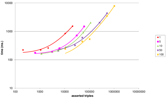
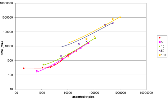
In order to analyze the results, the behaviour of the prototype for each of the rulesets has been plotted to graphs, shown in Figure 1. Each of the series represents a set with a fixed number of contexts (1 to 100) and each point a CKR. The $x$ axis represents the number of asserted triples, while the $y$ axis shows the time in milliseconds; the red horizontal line depicts the 30 minutes limit for timeout. To better visualize the behaviour of the series, we plotted a trend line for each of the series: the lines represent an approximation of the data trend calculated by polynomial regression.

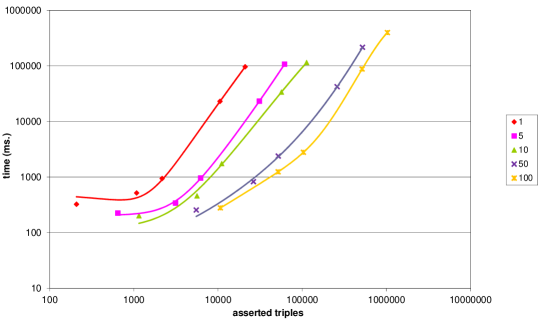a) ckr-rdfs-global	b) ckr-owl-global
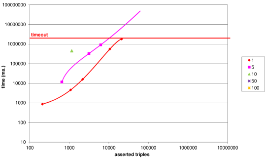c) ckr-rdfs-local	d) ckr-owl-local

Figure 1: Scalability graphs for TS1.

Some conclusions can be derived from these data and graphs: the first most evident fact is that the reasoning regime strongly impacts the scalability of the system. Thus, in practical cases the choice of a naive application of the full OWL RL ruleset might not be viable, in presence of large local datasets: on the other hand, if expressive reasoning inside contexts is not required, scalability can be enhanced by relying on the RDFS rulesets (or, in general, by carefully tailoring the ruleset to the required expressivity).

By analyzing the graphs and the approximations, it is also possible to observe that the system shows a different behaviour depending on the different reasoning regimes. In the case of ckr-rdfs-global and ckr-owl-global, the results suggest that the management of named graphs does not add overhead to the reasoning in the global context. This can be also seen by checking Table 3: for a similar number of inferred triples the separation across different graphs does not influence the reasoning time. For example, this is visible for cases with similar $y$ values of the graph (e.g. the case for 1000 classes in series for 1 and 5 contexts, in both rulesets). In the case of ckr-rdfs-local, the graphs show that local reasoning clearly influences the total inference time. In particular, at the growth of number of contexts, the behaviour tends to be linear in the number of asserted triples. While the data we have on ckr-owl-local are more limited, this behaviour seems to be confirmed by the trend lines. On the other hand, OWL local reasoning seems to influence the reasoning time with respect to the RDFS case: informally, this can be seen in the graph by the larger time overhead across points with a similar number of asserted triples (i.e. on the same $x$ values) but a higher number of contexts.

TS2 and TS3: knowledge propagation evaluation. The second set of experiments we carried out was aimed at answering question RQ2: we wanted to establish the cost of knowledge propagation among contexts, with respect to an increasing number of connections (i.e. eval expressions) across contexts. To this aim, we generated two test sets, called TS2 and TS3 structured as follows:

• TS2 is composed by 100 CKRs, each of them with 100 contexts. Except for the triples needed for the definition of the contextual structure, both the global and local knowledge bases contain no randomly generated axioms. The CKRs inside TS2 are generated with an increasing number of contexts connections trough eval axioms (from no connections to the case of “fully connected” contexts). In particular, for $n=100$ contexts and $k$ connections, in each context $c_{i}$ we add axioms of the kind:

  $$\textsl{eval}(D_{0},\{c_{i+1(mod\ n)}\})\sqsubseteq D_{1},\ \dots,\ \textsl{eval}(D_{0},\{c_{i+k(mod\ n)}\})\sqsubseteq D_{1}$$

  Moreover, in each context we add a fixed number of instances (10 in the case of TS2) of the local concept $D_{0}$, that will be propagated through contexts and added to local $D_{1}$ concepts by the inference rules for the above eval expressions.

• TS3 analogously contains 100 CKRs of 100 contexts and again no randomly generated global or local axioms. Differently from TS2, TS3 contains no eval axioms and the connections across contexts are simulated by having multiple versions of $D_{0}$ (namely $D_{0\text{-}0},\dots,D_{0\text{-}99}$) to represent the local interpretation of the concept. Thus, for $n=100$ contexts and $k$ connections, in each context $c_{i}$ we add axioms of the kind $D_{0\text{-}j}\sqsubseteq D_{1}$ for $j\in\{i+1(mod\ n),\dots,i+k(mod\ n)\}$. Also, not only we add to $c_{i}$ the 10 local instances of $D_{0\text{-}i}$, but we also “pre-propagate” instances of each $D_{0\text{-}j}$ by explicitly adding them to the knowledge of $c_{i}$.

We remark that the way of expressing “contextualized symbols” used in TS3 has been discussed and compared to the CKR representation in [1].

	TS2				TS3
Related	Triples	Total	Inf.	Time	Triples	Total	Inf.	Time
0	2803	3305	502	276	2803	3305	502	299
4	4703	9205	4502	893	11703	16205	4502	577
9	6703	16205	9502	1564	22703	32205	9502	1017
14	8703	23205	14502	2245	33703	48205	14502	1450
19	10703	30205	19502	2932	44703	64205	19502	1960
24	12703	37205	24502	3467	55703	80205	24502	2580
29	14703	44205	29502	4196	66703	96205	29502	3154
34	16703	51205	34502	4847	77703	112205	34502	4099
39	18703	58205	39502	5987	88703	128205	39502	4645
44	20703	65205	44502	6223	99703	144205	44502	5488
49	22703	72205	49502	6878	110703	160205	49502	6456
54	24703	79205	54502	7689	121703	176205	54502	7545
59	26703	86205	59502	8547	132703	192205	59502	8205
64	28703	93205	64502	9076	143703	208205	64502	9159
69	30703	100205	69502	9640	154703	224205	69502	10335
74	32703	107205	74502	10711	165703	240205	74502	10992
79	34703	114205	79502	11223	176703	256205	79502	11879
84	36703	121205	84502	14611	187703	272205	84502	13088
89	38703	128205	89502	12846	198703	288205	89502	13912
94	40703	135205	94502	14999	209703	304205	94502	15064
99	42703	142205	99502	14107	220703	320205	99502	15799

Table 4: Knowledge propagation results (extract) for test set TS2 and TS3.

We ran the CKR prototype for 5 independent runs on TS2 and TS3, only considering ckr-owl-local ruleset. An extract of the results of experiments on the two test sets is reported in Table 4: CKRs in the two sets are ordered with respect to the number of relations across contexts; for each CKR, the numbers of asserted, total and inferred triples are shown, followed by the (average) closure time in milliseconds. To facilitate the analysis of the results, we plotted such data in histograms in Figure 2. The $x$ axis represents the number of local connections, while the $y$ axis shows the time in milliseconds. Again, to better visualize the behaviour of the series, we plotted a trend line for each of the series, calculated by polynomial regression.

Figure 2: Knowledge propagation graphs for TS2 and TS3.

From the graph of TS2, we can note that knowledge propagation cost depends linearly on the number of connections: from the data in Table 4 we can calculate that the average increase in closure time for $k$ local connections (for each context) w.r.t. the base case of 0 connections amounts to $(51,\!2\cdot k)\%$. The comparison with TS3 confirms the compactness of a contextualized representation of symbols (cfr. findings in [1]): in fact, note that for an equal number of connections, the number of inferences in both TS2 and TS3 cases is equal, but TS3 always require a larger number of asserted triples. Also, the graph clearly shows that TS3 grows more than linearly: for a small number of connections the knowledge propagation in TS2 requires more inference time ($14,\!9\%$ more, on average), but with the growth of local connections (at $\sim\!68\%$ of number of contexts) the cost of TS3 local reasoning surpasses the propagation overhead.

5 Conclusions and Future Works

In this paper we provided a first evaluation for the performance of the RDF based implementation of the CKR framework. In first experiment we evaluated the scalability of the current version of the prototype under different reasoning regimes. The second experiment was aimed at evaluating the cost of intra-context knowledge propagation and its relation to its simulation by “reification” of contextualized symbols.

Some further experimental evaluations can be interesting to be carried out over our contextual model: one of these can regard the study of the cost and advantages of the separation of the same amount of knowledge across different contexts. With respect to the current CKR implementation, the scalability experiments clearly showed that the current naive strategy (defined by a direct translation of the formal calculus) might not be suitable for a real application of the full reasoning to large scale datasets. In this regard, we are going to study different evaluation strategies and optimizations to the current strategy and evaluate the results with respect to the naive case. One of such possible optimizations can regard a “pay-as-you-go” strategy, in which inference rules are activated only for constructs that are recognized in the local language of a context.

References

- [1] Bozzato, L., Ghidini, C., Serafini, L.: Comparing contextual and flat representations of knowledge: a concrete case about football data. In: K-CAP 2013. pp. 9–16. ACM (2013)
- [2] Bozzato, L., Eiter, T., Serafini, L.: Contextualized Knowledge Repositories with Justifiable Exceptions. In: DL2014. CEUR-WP, vol. 1193, pp. 112–123. CEUR-WS.org (2014)
- [3] Bozzato, L., Homola, M., Serafini, L.: Towards More Effective Tableaux Reasoning for CKR. In: DL2012. CEUR-WP, vol. 824, pp. 114–124. CEUR-WS.org (2012)
- [4] Bozzato, L., Serafini, L.: Materialization Calculus for Contexts in the Semantic Web. In: DL2013. CEUR-WP, vol. 1014. CEUR-WS.org (2013)
- [5] Khriyenko, O., Terziyan, V.: A framework for context sensitive metadata description. IJSMO 1(2), 154–164 (2006)
- [6] Klarman, S.: Reasoning with Contexts in Description Logics. Ph.D. thesis, Free University of Amsterdam (2013)
- [7] Krötzsch, M.: Efficient inferencing for OWL EL. In: JELIA 2010. Lecture Notes in Computer Science, vol. 6341, pp. 234–246. Springer (2010)
- [8] Motik, B., Fokoue, A., Horrocks, I., Wu, Z., Lutz, C., Grau, B.C.: OWL 2 Web Ontology Language Profiles. W3C recommendation, W3C (Oct 2009), http://www.w3.org/TR/2009/REC-owl2-profiles-20091027/
- [9] Serafini, L., Homola, M.: Contextualized knowledge repositories for the semantic web. J. of Web Semantics 12 (2012)
- [10] Straccia, U., Lopes, N., Lukácsy, G., Polleres, A.: A general framework for representing and reasoning with annotated semantic web data. In: AAAI 2010. AAAI Press (2010)
- [11] Tanca, L.: Context-Based Data Tailoring for Mobile Users. In: BTW 2007 Workshops. pp. 282–295 (2007)
- [12] Udrea, O., Recupero, D., Subrahmanian, V.S.: Annotated RDF. ACM Trans. Comput. Log. 11(2), 1–41 (2010)