Semihard processes with BLM renormalization scale setting

Abstract

We apply the BLM scale setting procedure directly to amplitudes (cross sections) of several semihard processes. It is shown that, due to the presence of $\beta_{0}$-terms in the NLA results for the impact factors, the obtained optimal renormalization scale is not universal, but depends both on the energy and on the process in question. We illustrate this general conclusion considering the following semihard processes: (i) inclusive production of two forward high-$p_{T}$ jets separated by large interval in rapidity (Mueller-Navelet jets); (ii) high-energy behavior of the total cross section for highly virtual photons; (iii) forward amplitude of the production of two light vector mesons in the collision of two virtual photons.

1 Introduction

We discuss the application of the BFKL method BFKL to the description of semihard processes, i.e. processes in the kinematic region where the energy variable $s$ is substantially larger than the hard scale $Q^{2}$, namely $s\gg Q^{2}\gg\Lambda^{2}_{\rm QCD}$, where $Q$ is the typical transverse momentum and $\Lambda_{\rm QCD}$ is the QCD scale.

The BFKL approach allows to resum systematically in all orders of perturbation series the terms enhanced by leading logarithms of energy, $\alpha_{s}^{n}\ln^{n}(s/Q^{2})$ (leading logarithmic approximation or LLA) and sub-leading ones, $\alpha_{s}^{n+1}\ln^{n}(s/Q^{2})$ (next-to-LLA or NLA). The practical application of BFKL to physical processes encounters serious difficulties due to large NLA corrections and big renormalization scale setting uncertainties. Due to that, one needs to apply some optimization method to the QCD perturbative series. We adopt here the Brodsky-Lepage-Mackenzie (BLM) approach BLM that eliminates the renormalization scale ambiguity by absorbing the non-conformal $\beta_{0}$-terms into the running coupling. In particular, we apply this optimization method to (i) the production of two forward high-$p_{T}$ jets separated by a large interval in rapidity (Mueller-Navelet jets MN ), (ii) the total cross section for the collision of two off-shell photons with large virtualities and (iii) the forward amplitude for the electroproduction of two light vector mesons.

2 BFKL amplitude and BLM scale setting

Within the class of semihard processes, we are interested in the study of physical observables directly related to the forward amplitude. One of these observables is the cross section itself that, due to the optical theorem, can be written as $\sigma=\frac{{\rm Im}_{s}{\cal A}}{s}$.

In the BFKL approach, both in the LLA and in the NLA, ${\rm Im}_{s}{\cal A}$ is given as the convolution of the Green’s function ($G_{\omega}$) of two interacting Reggeized gluons with momenta $q_{1,2}$ and of the impact factors of the colliding particles ($\Phi_{1}$ and $\Phi_{2}$):

$${\rm Im}_{s}\left({\cal A}\right)=\frac{s}{(2\pi)^{2}}\int\frac{d^{2}\vec{q}_{1}}{\vec{q}_{1}^{\,\,2}}\Phi_{1}(\vec{q}_{1},s_{0})\int\frac{d^{2}\vec{q}_{2}}{\vec{q}_{2}^{\,\,2}}\Phi_{2}(-\vec{q}_{2},s_{0})\int\limits^{\delta+i\infty}_{\delta-i\infty}\frac{d\omega}{2\pi i}\left(\frac{s}{s_{0}}\right)^{\omega}G_{\omega}(\vec{q}_{1},\vec{q}_{2})\,,$$ (1)

where $s$ is the squared center-of-mass energy of the colliding particles, while $s_{0}$ is an artificial scale introduced in the BFKL approach to perform the Mellin transform from the $s$-space to the complex angular momentum plane. Moving to the $(n,\nu)$-representation, which means using the basis of the eigenfunctions of the leading-order (LO) BFKL kernel instead of that of transverse momenta, we get

$${\rm Im}_{s}\left({\cal A}\right)=\frac{s}{(2\pi)^{2}}\sum^{\infty}_{n=-\infty}\int\limits^{\infty}_{-\infty}d\nu\left(\frac{s}{s_{0}}\right)^{\bar{\alpha}_{s}(\mu_{R})\chi(n,\nu)}\alpha_{s}^{2}(\mu_{R})c_{1}(n,\nu)c_{2}(n,\nu)\left\{1+\bar{\alpha}_{s}(\mu_{R})\left(\frac{c^{(1)}_{1}(n,\nu)}{c_{1}(n,\nu)}+\frac{c^{(1)}_{2}(n,\nu)}{c_{2}(n,\nu)}\right)\right.$$

$$\left.+\bar{\alpha}^{2}_{s}(\mu_{R})\ln\frac{s}{s_{0}}\left[\bar{\chi}(n,\nu)+\frac{\beta_{0}}{8N_{c}}\chi(n,\nu)\left(-\chi(n,\nu)+\frac{10}{3}+2\ln\mu_{R}^{2}+i\frac{d}{d\nu}\ln\frac{c_{1}(n,\nu)}{c_{2}(n,\nu)}\right)\right]\right\}\;.$$ (2)

The cross section could be represented, accordingly, as

$$\sigma=\frac{1}{\left(2\pi\right)^{2}}\left[C_{0}+\sum_{n=1}^{\infty}2\cos\left(n\phi\right)C_{n}\right]\,.$$ (3)

Here $c_{i=1,2}(n,\nu)$ and $c_{i=1,2}^{(1)}(n,\nu)$ are the impact factors at the LO and next-to-LO (NLO) in the $(n,\nu)$-representation, respectively; $\chi(n,\nu)$ is the LO BFKL characteristic function and $\bar{\chi}(n,\nu)$ is related with the NLO correction to the BFKL kernel. For more details on the derivation of Eq. (2), see e.g. Ref. BLM_paper . Note that $C_{0}$ is the total cross section, while the $C_{n}$’s with $n\neq 0$ are associated to azimuthal angle correlations, as in the case of Mueller-Navelet jets.

According to the BLM method, the renormalization scale $\mu_{R}$ in an the expression for a certain observable is chosen such that it makes the $\beta_{0}$-dependent part vanish. For the observable $C_{n}$, originally given in the $\overline{\rm MS}$ scheme, we first perform a finite renormalization transformation to the physical MOM scheme, which implies the replacement

$$\alpha_{s}^{\overline{\rm MS}}=\alpha_{s}^{\rm MOM}\left(1+\frac{\alpha_{s}^{\rm MOM}}{\pi}T\right)\;,\;\;\;\;\;T=T^{\beta}+T^{\rm conf}\;,$$ (4)

$$T^{\beta}\ =\ -\frac{\beta_{0}}{2}\left(1+\frac{2}{3}I\right)\;,\;\;\;\;\;T^{\rm conf}\ =\ \frac{C_{A}}{8}\left[\frac{17}{2}I+\frac{3}{2}\left(I-1\right)\xi+\left(1-\frac{1}{3}I\right)\xi^{2}-\frac{1}{6}\xi^{3}\right]\;,$$

where $I=-2\int_{0}^{1}dx\frac{\ln\left(x\right)}{x^{2}-x+1}\simeq 2.3439$ and $\xi$ is a gauge parameter. We thus get

$$C^{\rm MOM}_{n}=\frac{1}{(2\pi)^{2}}\int\limits^{\infty}_{-\infty}d\nu\left(\frac{s}{s_{0}}\right)^{\bar{\alpha}^{\rm MOM}_{s}(\mu_{R})\chi(n,\nu)}\left(\alpha^{\rm MOM}_{s}(\mu_{R})\right)^{2}c_{1}(n,\nu)c_{2}(n,\nu)$$

$$\times\left[1+\bar{\alpha}^{\rm MOM}_{s}(\mu_{R})\left\{\frac{\bar{c}^{(1)}_{1}(n,\nu)}{c_{1}(n,\nu)}+\frac{\bar{c}^{(1)}_{2}(n,\nu)}{c_{2}(n,\nu)}+\frac{2T^{\rm conf}}{N_{c}}+\frac{\tilde{c}_{1}^{(1)}}{c_{1}}+\frac{\tilde{c}_{2}^{(1)}}{c_{2}}\right\}\right.$$ (5)

$$+\left(\bar{\alpha}^{\rm MOM}_{s}(\mu_{R})\right)^{2}\ln\frac{s}{s_{0}}\left\{\!\bar{\chi}(n,\nu)+\frac{T^{\rm conf}}{N_{c}}\chi(n,\nu)\left.+\frac{\beta_{0}}{4N_{c}}\chi(n,\nu)\left(\!-\frac{\chi(n,\nu)}{2}+\frac{5}{3}+\ln\frac{\mu_{R}^{2}}{Q_{1}Q_{2}}+f(\nu)-2\left(1+\frac{2}{3}I\right)\right)\right\}\right]\,,$$

where $\tilde{c}_{1,2}^{(1)}$ represent the part of the impact factor depending on $\beta_{0}$, while $\bar{c}_{1,2}^{(1)}$ is the rest. In particular, the contribution to the NLO impact factor that is proportional to $\beta_{0}$ is universally expressed through the lowest order impact factors,

$$\frac{\tilde{c}_{1}^{(1)}}{c_{1}}+\frac{\tilde{c}_{2}^{(1)}}{c_{2}}\ =\ \frac{\beta_{0}}{2N_{c}}\left[\frac{5}{3}+\ln\frac{\mu_{R}^{2}}{Q_{1}Q_{2}}+f(\nu)\right]\;,$$ (6)

where the function $f(\nu)$ depends on the process considered and is given by

$$i\frac{d}{d\nu}\ln\left(\frac{c_{1}}{c_{2}}\right)\equiv 2\left[f(\nu)-\ln\left(Q_{1}Q_{2}\right)\right]\;.$$

Here $Q_{1,2}$ denotes the hard scale which enters impact factor $c_{1,2}$.

Now the optimal scale $\mu_{R}^{\rm BLM}$ is chosen such that it makes the expression proportional to $\beta_{0}$ vanish:

$$C^{\beta}_{n}=\frac{1}{(2\pi)^{2}}\int\limits^{\infty}_{-\infty}d\nu\left(\frac{s}{s_{0}}\right)^{\bar{\alpha}^{\rm MOM}_{s}(\mu^{\rm BLM}_{R})\chi(n,\nu)}\left(\alpha^{\rm MOM}_{s}(\mu^{\rm BLM}_{R})\right)^{3}$$

$$\times c_{1}(n,\nu)c_{2}(n,\nu)\frac{\beta_{0}}{2N_{c}}\left[\frac{5}{3}+\ln\frac{(\mu^{\rm BLM}_{R})^{2}}{Q_{1}Q_{2}}+f(\nu)-2\left(1+\frac{2}{3}I\right)\right.$$ (7)

$$\left.+\bar{\alpha}^{\rm MOM}_{s}(\mu^{\rm BLM}_{R})\ln\frac{s}{s_{0}}\frac{\chi(n,\nu)}{2}\left(-\frac{\chi(n,\nu)}{2}+\frac{5}{3}+\ln\frac{(\mu^{\rm BLM}_{R})^{2}}{Q_{1}Q_{2}}+f(\nu)-2\left(1+\frac{2}{3}I\right)\right)\right]=0\;.$$

Unfortunately, Eq. (7) can be solved only numerically. Therefore here we will limit ourselves to approximate approaches to the BLM scale setting. We consider the BLM scale as a function of $\nu$ and choose it in order to put equal to zero either the terms in the second line of Eq. (7) (case $(a)$) or those in the third line of the same equation (case $(b)$). This corresponds to the vanishing of the $\beta_{0}$-terms originating from the NLO corrections of the impact factors or of the BFKL kernel, respectively. We have then the two following cases:

$$\left(\mu_{R,a}^{\rm BLM}\right)^{2} = Q_{1}Q_{2}\ \exp\left[2\left(1+\frac{2}{3}I\right)-f\left(\nu\right)-\frac{5}{3}\right]\;,$$ (8)

$$\left(\mu_{R,b}^{\rm BLM}\right)^{2} = Q_{1}Q_{2}\ \exp\left[2\left(1+\frac{2}{3}I\right)-f\left(\nu\right)-\frac{5}{3}+\frac{1}{2}\chi\left(\nu,n\right)\right]\;.$$ (9)

3 Application to some semihard processes

Now we test the two solutions, Eqs. (8) and (9), on different semihard processes: (i) the inclusive production of Mueller-Navelet jets, (ii) the collision of two highly-virtual photons at large energies and (iii) the production of two light vector mesons in the collision of two virtual photons, $\gamma^{*}\gamma^{*}\to V_{1}V_{2}$.

For these particular processes we have $f(\nu)=0$ in the first two cases, while $f(\nu)\ =\ \psi\left(3+2i\nu\right)+\psi\left(3-2i\nu\right)-\psi\left(\frac{3}{2}+i\nu\right)-\psi\left(\frac{3}{2}-i\nu\right)$ for the case of meson pair production.

Some of our results are reported in Fig. 1. In particular we show the forward amplitude for the $\gamma^{*}\gamma^{*}\to V_{1}V_{2}$ process and the cross section of the Mueller-Navelet jets production process as a function of the rapidity interval between the produced pair of mesons or jets. For the explicit definition of the considered quantities, see Ivanov:2005gn and jet_paper , correspondingly.

Other results for Mueller-Navelet jets, including moments of azimuthal angular correlations between jets, can be found in Fig. 3 of jet_paper .

Our results for the application of BLM method to the high-energy behavior of the total cross section for highly virtual photons is given instead in Fig. 6 of photon_paper (see also Caporale:2008is ).

4 Discussion

We note that in all cases the NLA corrections are very large and important. To illustrate this statement, we show in Fig. 1 also the LLA contributions, calculated for natural (i.e. non-optimal) choices of the energy and renormalization scales. Due to this fact, NLA predictions for semihard processes depend substantially on the choice of energy scale $s_{0}$ and on the value of renormalization scale $\mu_{R}$. We adopted here the BLM procedure to fix $\mu_{R}$.

The application of the BLM approach to semihard reactions was pioneered in Brodsky:1998kn , where the method was applied to calculate the intercept of the BFKL Pomeron in the NLO. Later on, in Brodsky:2002ka the total cross section of $\gamma^{*}\gamma^{*}$ interactions at high energy was studied. Recently it was shown in Ducloue:2013bva that the application of the BLM method leads to a successful phenomenology of Mueller-Navelet jet production at LHC.

One should mention, however, that the implementation of the BLM method in Brodsky:2002ka ; Ducloue:2013bva was approximate, because it did not take into account the $\beta_{0}$-dependent parts of the NLA forward amplitudes originating from the NLO impact factors. Instead, only contributions coming from the NLO corrections to the BFKL kernel were considered, which corresponds to our case $(b)$, given in Eq. (9). Our case $(a)$, see (8), means instead the approximation when one takes into account the $\beta_{0}$-terms coming only from the impact factors and neglects those originating from the kernel.

Note that an explicit solution of the BLM scale setting equation (7) leads to optimal scale values which depend on the process energy, $s$. To some extent, the explicit solution of (7) gives a scale that interpolates between the approximate ones presented in (8) and (9). Note also the BLM scale derived from (7) is not universal, but depends on the process in question, through the form of the LO impact factors, $c_{1,2}(n,\nu)$.

We observe that the difference of the two predictions for the Mueller-Navelet jet production cross section derived here using the approximate choices $(a)$ and $(b)$ of the BLM scale is not big. In our forthcoming paper BLM_paper we will present results for this and other Mueller-Navelet observables obtained also with the “exact” determination of BLM scale, as defined by Eq. (7). We will study also the dependence of the predictions obtained with BLM method on the variation of the energy scale parameter $s_{0}$.

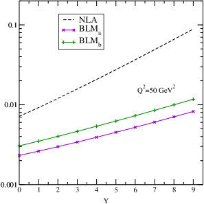
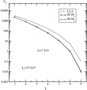
Figure 1: Forward amplitude for the process $\gamma*\gamma*\to V_{1}V_{2}$ (left) and cross section of $p+p\to\textup{jet}+\textup{jet}+X$ (right).

References

- (1) V.S. Fadin, E.A. Kuraev, L.N. Lipatov, Phys. Lett. B 60 (1975) 50; E.A. Kuraev, L.N. Lipatov, V.S. Fadin, Zh. Eksp. Teor. Fiz. 71 (1976) 840; 72 (1977) 377; Ya.Ya. Balitskii, L.N. Lipatov, Sov. J. Nucl. Phys. 28 (1978) 822.
- (2) S.J. Brodsky, G.P. Lepage, P.B. Mackenzie, Phys. Rev. D 28 (1983) 228.
- (3) A.H. Mueller, H. Navelet, Nucl. Phys. B 282 (1987) 727.
- (4) F. Caporale, D.Yu. Ivanov, B. Murdaca, A. Papa, On the BLM optimal renormalization scale setting for semihard processes, in preparation.
- (5) D.Yu. Ivanov and A. Papa, Nucl. Phys. B 732 (2006) 183.
- (6) F. Caporale, D.Yu. Ivanov, B. Murdaca, A. Papa, Eur. Phys. J. C 74 (2014) 10, 3084.
- (7) D.Yu. Ivanov, B. Murdaca, A. Papa, JHEP 1410 (2014) 58.
- (8) F. Caporale, D.Yu. Ivanov and A. Papa, Eur. Phys. J. C 58 (2008) 1.
- (9) S.J. Brodsky, V.S. Fadin, V.T. Kim, L.N. Lipatov and G.B. Pivovarov, JETP Lett. 70 (1999) 155.
- (10) S.J. Brodsky, V.S. Fadin, V.T. Kim, L.N. Lipatov and G.B. Pivovarov, JETP Lett. 76 (2002) 249 [Pisma Zh. Eksp. Teor. Fiz. 76 (2002) 306].
- (11) B. Ducloué, L. Szymanowski and S. Wallon, Phys. Rev. Lett. 112 (2014) 082003.