Holographic thermalization of charged operators

Abstract

We study a light-like charged collapsing shell in AdS-Reissner-Nordstrom spacetime, investigating whether the corresponding Vaidya metric is supported by matter that satisfies the null energy condition. We find that, if the absolute value of the charge decreases during the collapse, energy conditions are fulfilled everywhere in spacetime. On the other hand, if the absolute value of the charge increases, the metric does not satisfy energy conditions in the IR region. Therefore, from the gauge/gravity perspective, this last case is only useful to study the thermalization of the UV degrees of freedom. For all these geometries, we probe the thermalization process with two point correlators of charged operators, finding that the thermalization time grows with the charge of the operator, as well as with the dimension of space.

I Introduction

The study of non-equilibrium processes in quantum field theory is an important and active area of research (see noneq for references). The subject has most diverse applications that range from astrophysics and cosmology, i.e. the study of particle production at the end of inflation and the generation of density fluctuations, to relativistic heavy ion collisions, i.e. the dynamics of the quark-gluon plasma at RHIC. For the case of near-equilibrium states there exist well developed formalisms: linear response, kinetic theory or fluid dynamics. This techniques rely on the existence of a dilute equilibrium ensemble or weak coupling. However in many physical instances the system to be studied can be strongly coupled or in a dense state or both, and therefore in these situations the standard techniques do not apply.

The question of whether a given subset of the degrees of freedom of a certain system reaches equilibrium starting from an arbitrary initial state, and whether such equilibrium can be described by a thermal density matrix, is an open one whose answer seems to depend on the details of the underlying dynamics nonequil2 . A large number of numerical and analytical research on such quenching process has been published (see quenches and references therein), regarding both weakly coupled systems in the perturbative regime nonequil-peturbative , and integrable systems nonequil-integrable . Moreover, strong coupling QFT’s have been studied numerically in the lattice nonequil-lattice .

In this paper we will consider the study of far from equilibrium strongly coupled systems using the gauge/gravity correspondence. As it is well known, the holographic correspondence is the natural arena for analyzing strongly coupled QFT problems translating them into classical gravity computations. For near-equilibrium states, the correspondence has been extensively studied with particular emphasis in the linear response and the hydrodynamic regime, in terms of perturbations of the black hole geometry (see the recent reviews hube ; HotQCD ). More recently, attention has been paid to far-from-equilibrium states. Reference bala made a holographic proposal to model the sudden injection of energy into the QFT vacuum state, and its subsequent thermalization, in terms of an AdS Vaidya geometry. The dynamical Vaidya spacetime physically corresponds to the collapse of a homogeneous massless shell in AdS, leading to the formation of a black hole Vaidya1 . It interpolates between pure AdS spacetime (vacuum) in the distant past to an AdS black hole (thermal state) in the distant future. Two point functions of operators $\cal O$ of large conformal dimensions, which in the dual picture can be computed in the semiclassical approximation in terms of geodesics, and Wilson loops and entanglement entropy, which in the gravity perspective relate to minimal (hyper)surfaces, were used as probes of thermalization. The resulting picture is that the UV degrees of freedom thermalize first, followed later by the IR ones (top-down thermalization bala ). From the gravity perspective this is an expected result since IR probes explore deeply in the radial direction being therefore sensitive to the shell position for longer times.

The aforementioned results were generalized in martin ; subad to situations with a non-trivial chemical potential or, in the dual perspective, to the case in which the system experiences a sudden injection of both energy and particles. The dual geometry was chosen to be that of a charged collapsing null shell interpolating between AdS in the distant past and asymptotically AdS Reissner-Nordstrom black hole (AdSRN) in the distant future. The thermalization was probed by two point functions of chargeless operators, Wilson loops, and entanglement entropy. The emergent picture of martin was that as the final chemical potential is increased, it takes longer for the system to thermalize (see Garfinkle -elena2 for related works).

It is the aim of the present paper to extend the studies mentioned above. In particular, since the Vaidya geometry is known to be supported by an energy-momentum tensor satisfying null energy conditions, in the present work we analyze the energy conditions of the previously explored charged Vaidya geometries martin ; subad and its further generalizations. We afterwards study the thermalization process by probing the system with charged operators.

The organization of the paper is the following: In section II we analyze whether the Vaidya metric used in martin ; subad , that represents a quench on the chemical potential and temperature in the dual field theory, is supported by matter satisfying null energy conditions, in section III we probe the thermalization process with two point functions of charged operators. The results are presented and discussed in section IV. We conclude with a summary in section V. In the appendices we discuss Eddingtong-Finkelstein coordinates, the worldline formalism and the WKB approximation, used in the text to obtain the two-point functions of charged operators.

II Background geometry

The gauge/gravity duality relates a strongly coupled quantum field theory (QFT) in $d$ flat spacetime dimensions with a weakly coupled gravity theory in a $d+1$ dimensional spacetime which asymptotes to anti-de Sitter spacetime. According to the standard gauge/gravity dictionary, a finite temperature state of the field theory is represented by a geometry with a horizon in the bulk side. Moreover, a global symmetry in the field theory induces a gauge symmetry in the gravity side. As a consequence, the presence of a chemical potential for a global $U(1)$ charge at finite temperature on the QFT side is described in the dual gravitational picture by the presence of an electrically charged black hole [hartnoll, ]. In the simplest example, an equilibrium state with finite temperature and chemical potential is represented by an AdSRN black hole with given mass and charge. On the other hand, a process in which the temperature and chemical potential vary can be represented by a metric which interpolates between two such geometries with different values of mass and charge. In this section, we describe those geometries and analyze the energy momentum tensor that is needed to support them. We model the dynamical geometry by the collapse of a thin shell of null dust. It turns out to be convenient to substitute the standard time coordinate $t$, which is not constant across the shell, by an infalling radial null coordinate $v$ which is.

In what follows, we take $d$ to be the spacetime dimension of the dual field theory, hence our bulk geometry will be $d+1$ dimensional. The indices $\mu,\nu=0\dots d$ denote the bulk coordinates $x^{\mu}=(v,{\bf x},z)$.

II.1 Equilibrium state

Bulk geometry

In Eddington-Finkelstein ingoing null coordinates, the metric and gauge fields corresponding to a planar AdS_d+1 Reissner-Nordstrom black hole take the form (see appendix A)

$$ds^{2} = \frac{L^{2}}{z^{2}}\left(-fdv^{2}-2dvdz+d{\bf x}^{2}_{d-1}\right)\,,$$ (1)

$$F = L\,F_{zv}\,dz\wedge dv\,,$$ (2)

where $f$ and $F_{zv}$ are functions of $z$ that read

$$f = 1-Mz^{d}+Q^{2}z^{2(d-1)}\,,$$ (3)

$$F_{zv} = -\gamma(d\!-\!2){Q}z^{d-3},~{}~{}~{}~{}~{}~{}~{}~{}~{}~{}~{}~{}\mbox{with}~{}~{}~{}~{}~{}\gamma^{2}=\frac{d-1}{2(d-2)}\,.$$ (4)

The static background (1)-(2) is a vacuum solution of the $(d+1)$-dimensional Einstein-Maxwell system with negative cosmological constant $\Lambda=-{d(d-1)}/{2(\kappa L)^{2}}$

$$S_{EM}=\frac{1}{2\kappa^{2}}\int d^{d+1}x\sqrt{-g}\left[R+\frac{d(d-1)}{L^{2}}\right]-\frac{1}{4}\int d^{d+1}x\sqrt{-g}F_{\mu\nu}F^{\mu\nu}\,.$$ (5)

Setting $\kappa^{2}=1$ the equations of motion following from $S_{EM}$ are

$$R_{\mu\nu}-\frac{1}{2}g_{\mu\nu}R+\Lambda g_{\mu\nu} = T_{\mu\nu}^{\sf Maxwell},$$ (6)

$$\nabla_{\mu}F^{\mu\nu} = 0\,,$$ (7)

where

$$T_{\mu\nu}^{\sf Maxwell}=F_{\mu\alpha}F_{\nu\beta}g^{\alpha\beta}-\frac{1}{4}g_{\mu\nu}F^{2}\,.$$ (8)

The geometry (1) asymptotes AdS space with radius $L$ as we approach the boundary located at $z=0$, and the constants $M$ and $Q$ correspond to the ADM mass and electric charge respectively. The metric (1) has a curvature singularity at $z\to\infty$ and has horizons whenever the function $f$ vanishes. To characterize the horizons, notice that $f$ has two stationary points, one at $z=0$ at which $f=1$, and a second one (a local minimum) at $z_{min}=(d\,M/2(d-1)Q^{2})^{1/(d-2)}$. The curvature singularity will be hidden from the outside as long as $f(z_{min})\leq 0$, which implies a constraint on the possible values of $M,Q$

$$\left(\frac{M^{d-1}}{Q^{d}}\right)^{2}\geq\left(\frac{2(d-1)}{d}\right)^{d}\left(\frac{2(d-1)}{d-2}\right)^{d-2}\,.$$ (9)

Whenever this inequality is satisfied, we generically have two horizons at $z=z_{\pm}$ (inner/outer). Moreover, when the bound is saturated the two horizons coincide and the configuration is called an extremal black hole solution (more on this below). We will demand the constraint (9) on all our solutions in order to have a physically sensible gravitational background.

Although charged black holes generically depend on two arbitrary parameters $Q$ and $M$, this is not so in the planar horizon case. The absence of a scale on the horizon geometry allows us to get rid of one of the parameters. Explicitly, the rescaling $(v,{\bf x},z)=z_{-}(\tilde{v},\tilde{\bf x},\tilde{z})$ maps the (outer) horizon position to $\tilde{z}=1$. Defining $\tilde{M}=Mz_{-}^{d}$ and $\tilde{Q}=Qz_{-}^{d-1}$ one finds that $\tilde{M}=1+\tilde{Q}^{2}$ resulting into hartnoll

$$f = 1-(1+\tilde{Q}^{2})\tilde{z}^{d}+\tilde{Q}^{2}\tilde{z}^{2(d-1)}\,,$$ (10)

$$F_{zv} = -\gamma\,(d\!-\!2){\tilde{Q}}\tilde{z}^{d-3}\,.$$ (11)

This is the parametrization often used in the literature for the planar Reissner-Nordstrom AdS black hole. It automatically satisfies the constraint (9), and notice that $\tilde{Q}$ can take any arbitrary value. The geometry (10) has generically two horizons. Depending on the value of $\tilde{Q}$ one has: (i) an outer one at $\tilde{z}_{-}=1$ and an inner one at $\tilde{z}_{+}>1$ for $|\tilde{Q}|\leq\sqrt{d/{(d-2)}}$, (ii) coincident horizons at $\tilde{z}_{\pm}=1$ for $\tilde{Q}^{2}=d/(d-2)$ (extremal BH), and (iii) an inner horizon at $\tilde{z}_{+}=1$ and an outer one at $\tilde{z}_{-}<1$ for $|\tilde{Q}|>\sqrt{d/{(d-2)}}$. An appropriate rescaling of the holographic coordinate maps the type (iii) solutions to the type (i) ones.

Summarizing, the background (10)-(11) with $|\tilde{Q}|\leq\sqrt{d/{(d-2)}}$ parametrizes the most general static planar AdSRN solution with an outer horizon located at $\tilde{z}_{-}=1$ and an inner horizon located at $\tilde{z}_{+}\geq 1$.

Boundary theory

As mentioned above, the AdS boundary is located at $z=0$ and, as it is well known, the static geometry (1)-(2) represents a dual QFT equilibrium state characterized by a chemical potential $\mu$ and a temperature $\sf T$ hartnoll . The bulk variable $v$ is identified with the dual gauge theory time $t$ since both coincide at $z=0$ (see (12) below).

The standard procedure to relate the boundary and bulk parameters is to impose regularity of the Wick rotated solution. For the static case (3)-(4), the redefinition

$$-idt_{E}=dv+\frac{dz}{f}\,,$$ (12)

turns the geometry (1) into the Euclidean form

$$ds^{2} = \frac{1}{z^{2}}\left(fdt_{E}^{2}+\frac{dz^{2}}{f}+d{\bf x}^{2}_{d-1}\right)\,.$$ (13)

We note in passing that if the function $f$ were $v$-dependent, as it will become later when we define Vaidya metrics, the redefinition (12) would not be allowed, the right hand side being not an exact differential. The metric (13) is regular at the outer horizon $z=z_{-}$ if we periodically identify $t_{E}\equiv t_{E}+\beta$, with

$$\beta=\frac{4\pi}{|f_{z}(z_{-})|}\,,$$ (14)

the subindex $z$ on $f_{z}$ denotes derivative with respect to $z$. The boundary theory temperature is then defined as

$${\sf T}\equiv\frac{1}{\beta}=\frac{d\,Mz_{-}^{d}-2(d-1)Q^{2}z_{-}^{2d-2}}{4\pi z_{-}}\,.$$ (15)

Regarding the chemical potential of the boundary theory, it relates to the black hole charge as follows: we can choose the bulk gauge potential to be

$$A_{v}=-\gamma QL\,z^{d-2}+\mu L\,,$$ (16)

with $\mu$ arbitrary. From (12) one has $iA_{t_{E}}=-\gamma QLz^{d-2}+\mu L$. Since the $t_{E}$ circle smoothly collapses at the outer horizon, the gauge field must satisfy $A_{t_{E}}(z_{-})=0$ to avoid singularities. This condition fixes the asymptotic value of the gauge field to

$$\mu=\gamma Qz_{-}^{d-2}\,.$$ (17)

For a fixed mass black hole, increasing the chemical potential (i.e. the black hole charge) decreases the black hole temperature. The extremal bound in (9) corresponds to the ${\sf T}=0$ and $\mu\neq 0$ case. In the gauge/gravity duality context one identifies the gauge field boundary value $\mu$ as the source for the QFT conserved charge operator.

II.2 Time dependent states

Bulk geometry

To construct a time dependent geometry, we promote the $z$-dependent functions $f$ and $F_{zv}$ on (2) to $(z,v)$-dependent functions. In other words, we keep the ansatz for the metric and the field strength (1)-(2), but the functions $f,F_{zv}$ now depend on both variables $z,v$. Under this conditions, extra matter contributions $T_{\mu\nu}^{\sf Matter}$ and $j^{\mu}_{\sf Matter}$ need to be added to the right hand side of (6)-(7), in order to satisfy Einstein-Maxwell equations of motion. They physically represent an infalling charged matter shell giving birth to the black hole [Vaidya1, ]. The additional contribution to the energy momentum tensor is defined as

$$T_{\mu\nu}^{\sf Matter}=\left[G_{\mu\nu}-\frac{(d-1)d}{2L^{2}}\,g_{\mu\nu}\right]-T_{\mu\nu}^{\sf Maxwell}\,.$$ (18)

Working out the components of $T^{\sf Matter}_{\mu\nu}$ in terms of the functions $f,F_{zv}$ and their derivatives one finds

$$T_{vv}^{\sf Matter} = \frac{(d-1)}{2z^{2}}\bigg{(}f\big{(}\,zf_{z}-d\,f+d\big{)}-z\,f_{v}\bigg{)}-\frac{z^{2}}{2}\,fF_{zv}^{2}\,,$$ (19)

$$T_{vz}^{\sf Matter} = \frac{(d-1)}{2z^{2}}\bigg{(}z\,f_{z}-d\,f+d\bigg{)}-\frac{z^{2}}{2}\,F_{zv}^{2}\,,$$ (20)

$$T_{x_{i}x_{j}}^{\sf Matter} = \delta_{ij}\left[\frac{1}{2}f_{zz}-\frac{(d-1)}{2z^{2}}\bigg{(}2z\,f_{z}-d\,f+d\bigg{)}-\frac{z^{2}}{2}\,F_{zv}^{2}\right]\,.$$ (21)

In the right hand side of these expressions a subindex in $f$ denote partial derivative, $f_{v}\equiv\partial_{v}f$ and $f_{z}\equiv\partial_{z}f$.

A crucial point to be verified is whether the infalling matter that supports the time dependent solution satisfies appropriate energy conditions. In particular, the weakest energy condition that can be imposed is the so called null energy condition, that states that for any null vector $n^{\mu}$, the energy momentum tensor must satisfy

$$T_{\mu\nu}^{\sf Matter}n^{\mu}n^{\nu}\geq 0\,,$$ (22)

everywhere in spacetime. Writing a generic vector as $n^{\mu}=(n^{v},n^{z},n^{x},{\bf 0}_{d-2})$, where we have used the rotational invariance in the Cartesian coordinates ${\bf x}_{d-1}$ to eliminate redundant components, the condition for it to be null reads

$$g_{\mu\nu}n^{\mu}n^{\nu}=\frac{1}{z^{2}}(-f(n^{v})^{2}-2n^{v}n^{z}+(n^{x})^{2})=0\,.$$ (23)

This equation can be solved for $n^{z}$. There is one solution $n^{v}=n^{x}=0$ under which (22) vanishes identically imposing no constraint. On the other hand, when $n^{v}\neq 0$ the solution reads $n^{z}=((n^{x})^{2}-f(n^{v})^{2})/2n^{v}$, and upon replacing it into the energy condition (22) one finds

$$(T_{vv}^{\sf Matter}-fT_{vz}^{\sf Matter})(n^{v})^{2}+(T^{\sf Matter}_{xx}+T^{\sf Matter}_{vz})(n^{x})^{2}\geq 0\,.$$ (24)

In order for this quadratic form to be positive definite for any null vector, we need $(T_{vv}^{m}-fT_{vz}^{m})\geq 0$ and $(T^{m}_{xx}+T^{m}_{vz})\geq 0$, using (19)-(21) one finds

$$f_{v}\leq 0\,,$$ (25)

$$zf_{zz}-(d-1)f_{z}-2{z^{3}}\,F_{zv}^{2}\geq 0\,.$$ (26)

This set of equations constraint the $(z,v)$-dependence of the ansatz functions $f,F_{zv}$.

Another important requirement to be imposed on the solution is that any physical matter current sourcing the gauge fields must be time-like or null. Defining the matter current as

$$j^{\nu}_{\sf Matter} = \nabla_{\mu}F^{\mu\nu}$$ (27)

$$= \frac{1}{\sqrt{-g}}\,\partial_{\mu}\left(\sqrt{-g}F^{\mu\nu}\right)\,,$$

we find

$$j^{z}_{\sf Matter} = \frac{z^{4}}{L^{3}}F_{zv,v}\,,$$ (28)

$$j^{v}_{\sf Matter} = \frac{({d-3})z^{3}}{L^{3}}F_{zv}-\frac{z^{4}}{L^{3}}F_{zv,z}\,.$$ (29)

The matter current must satisfy

$$g_{\mu\nu}\,j^{\mu}_{\sf Matter}\,j^{\nu}_{\sf Matter}\leq 0\,,$$ (30)

or using (29)

$$\left(\frac{({d-3})}{z}F_{zv}-F_{zv,z}\right)\left(2F_{zv,v}+f\left(\frac{({d-3})}{z}F_{zv}-F_{zv,z}\right)\right)\geq 0\,.$$ (31)

We now consider the particular case where the $f,F_{zv}$ functions keep the same $z$-dependence as in (3)-(4), and $M$ and $Q$ become $v$-dependent functions $\hat{M}(v)$ and $\hat{Q}(v)$. As expected, this implies that the locus of zeros of $f$ (i.e. the horizon positions $\hat{z}_{\pm}$) will be $v$-dependent, and equations (28)-(29) imply that $j^{\mu}_{\sf Matter}=(0,j^{z}_{\sf Matter},{\bf 0}\,)$ with $j^{z}_{\sf Matter}$ given by (28). This matter current satisfies condition (30) as an equality, which means that the charged source for the gauge field is light-like. Moreover, the ensuing $T_{\mu\nu}^{\sf Matter}$ takes a null dust form, and the energy condition (26) is again satisfied as an equality. In passing, we notice that although we have a time dependent electric field, the matter current leads to no magnetic field in Ampere’s law. In summary, generalizing the ansatz to $v$-dependent functions $\hat{M}(v)$ and $\hat{Q}(v)$ in $f$ and $F_{zv}$ leads to a physically sensible gravity solution as long as they satisfy (25), which can be rewritten as

$$\hat{M}_{v}\geq 2\hat{Q}\hat{Q}_{v}z^{d-2}\,.$$ (32)

This energy condition (32) was discussed in martin ; subad . We would like to remark that (32) coincides with the condition for the horizon not the recede. Indeed, if we define the (time dependent) horizon position $\hat{z}_{h}$ as the solution to $f(\hat{z}_{h},v)=0$, we get $d\hat{z}_{h}/dv=-f_{v}/f_{z}\propto-\hat{M}_{v}+2\hat{Q}\hat{Q}_{v}z^{d-2}$, thus from the condition $d\hat{z}_{h}/dv\leq 0$ we obtain (32) (see Fig. 3 below). Nevertheless, condition (32) must be satisfied even in the absence of horizons.

We now turn to analyze its consequences:

• When the charge $\hat{Q}$ vanishes, (32) translates into

  $$\hat{M}_{v}\geq 0\,.$$ (33)

  Therefore, any interpolation between pure AdS and the planar AdS-Schwarzschild metric with a monotonically growing mass function, asymptotically reaching a constant value $M$, is a healthy solution of Einstein-Maxwell equations. The required additional matter contribution satisfies the null energy condition. The chargeless Vaidya metric case, used in bala to study thermalization of a strongly coupled plasma at zero chemical potential after an energy quench, allows for an arbitrary time pattern of energy injection (this is a well known result, and we mention it here only for completeness).

• If the charge remains constant as we perform the quench ($\hat{Q}_{v}=0$), condition (32) reduces to (33). As discussed above, the constraint (32) is identically satisfied as long as the mass function is monotonically increasing. The corresponding Vaidya geometry can be used to study thermalization processes at fixed chemical potential after an injection of energy.

• For non-constant charge situations, outside of the support of $\hat{Q}_{v}$, condition (32) reduces to (33). On the other hand, for analytic $\hat{Q}$ the support is non-compact, implying

  • Whenever $\hat{Q}\hat{Q}_{v}>0$, it is immediate to see that (32) is violated at large enough $z$ for any fixed value of $v$. Notice that $\hat{Q}\hat{Q}_{v}>0$ corresponds to an increasing absolute value of the charge, what we will call a “charging” background in what follows. The null energy condition therefore tell us that we can use a charging AdS Vaidya ansatz to study the thermalization of the dual field theory, as long as our probes explore the near boundary region. From the dual point of view this means that the geometry can only be trusted to describe the UV degrees of freedom of the field theory. These classes of solutions were used in martin ; subad to study the thermalization process after a quench on energy and chemical potential.

  • No additional constraint follows from (32) for the case of a “discharging” background $\hat{Q}\hat{Q}_{v}<0$, provided the mass is increasing $M_{v}>0$.

In summary, the charged metrics obtained by promoting the AdSRN charge and the mass into $v$-dependent functions (with growing mass), satisfy energy conditions everywhere in spacetime whenever they are “discharging” $\hat{Q}\hat{Q}_{v}<0$, while violate energy conditions in the bulk for large enough $z$, i.e. in the deep IR, whenever they are “charging” $\hat{Q}\hat{Q}_{v}>0$. In this last case probing the near boundary geometry is still a safe option. Note that in the above definitions, and throughout this paper, we use the words “charging” and “discharging” as referring to an increasing or decreasing absolute value of the charge.

In what follows, we use the aforementioned charging and discharging geometries in order to get information about the thermalization processes of the boundary theory. To such end, we choose our functions $\hat{M}$ and $\hat{Q}$ as interpolating between initial constant values $M_{\sf in}$ and $Q_{\sf in}$ in the asymptotic past $v\to-\infty$ and final constant values $M$ and $Q$ in the asymptotic future $v\to\infty$.

In the time-dependent background, the field strength in (2) can be obtained from the gauge potential

$$A_{v}=-\gamma\hat{Q}L\,z^{d-2}+\hat{\mu}L\,,$$ (34)

with $\hat{\mu}$ an arbitrary $v$-dependent function. The background $v$-dependence precludes the global definition of a time coordinate, since (12) is not an exact differential, avoiding an Euclidean continuation. Thus, the only constraint we impose on the function $\hat{\mu}$ arises from the regularity of the Euclidean continuation of the asymptotic regions $v\to\pm\infty$. In other words we choose $\hat{\mu}\to\gamma Q_{\sf in}z_{\sf in}^{d-2}$ when $v\to-\infty$, and $\hat{\mu}\to\gamma Qz_{h}^{d-2}$ when $v\to\infty$, where $z_{\sf in}$ and $z_{h}$ are the positions of the horizons before and after the quench.

Boundary theory

In the dual field theory, the proposed geometry describes a system interpolating between two different values of the temperature as the result of injecting energy homogeneously into the system, and at the same time quenching the chemical potential. The quench can take the chemical potential up or down depending on whether we have a charging or a discharging geometry, and corresponds to a homogeneous injection of particles/antiparticles into the system. Even if, as mentioned in the previous sections, there is no global time coordinate, with the hindsight of the static background we define a time coordinate in the asymptotic region $z\to 0$ as $t\sim v$: the variable $v$ at the boundary then coincides with the gauge theory time.

III Probes of thermalization

As a probe for analyzing the thermalization process, we study equal time two point correlators of charged scalar operators $\mathcal{O}_{\Delta}$ of conformal dimension $\Delta$. Decomposing the bulk coordinates as ${x}^{\mu}=(x^{\alpha},z)$, the AdS/CFT dictionary relates the QFT two point correlator $\langle\mathcal{O}_{\Delta}(x^{\alpha}_{1})\mathcal{O}_{\Delta}(x^{\alpha}_{2})\rangle$ to the Feynman propagator $G({x}_{1}^{\alpha},z_{1}|\,{x}^{\alpha}_{2},z_{2})$ of a charged scalar field of mass $m=\sqrt{\Delta(\Delta-d)}/L$ propagating in the bulk, according to the formula banks

$$\langle\mathcal{O}_{\Delta}(x^{\alpha}_{1})\mathcal{O}_{\Delta}(x^{\alpha}_{2})\rangle=\lim_{z_{1},z_{2}\to 0}\,z_{1}^{-\Delta}{z_{2}}^{-\Delta}G(x^{\alpha}_{1},z_{1}|\,x^{\alpha}_{2},z_{2})\,.$$ (35)

In the large mass limit $1\ll mL\approx\Delta$, the bulk propagator can be approximated by the classical trajectory (see appendix B)

$$G(x^{\alpha}_{1},z_{1}|\,x^{\alpha}_{2},z_{2})\approx e^{iS_{\sf on-shell}(x^{\alpha}_{1},z_{1}|\,x^{\alpha}_{2},z_{2})}\,,$$ (36)

with

$$S_{\sf on-shell}(x^{\alpha}_{1},z_{1}|\,x^{\alpha}_{2},z_{2})=\left.\int d\tau\left(-m\sqrt{-g_{\mu\nu}\dot{x}^{\mu}\dot{x}^{\nu}}+{\sf e}A_{\mu}\dot{x}^{\mu}\right)\right|_{x^{\mu}(\tau)=x^{\mu}_{\sf classical}(\tau)}\,.$$ (37)

Here $S_{\sf on-shell}$ is the appropriate action for the time-like trajectory, for a particle of mass $m$ and charge $\sf e$, evaluated on the classical trajectory $x^{\mu}_{\sf classical}(\tau)$ that joins $(x_{1}^{\alpha},z_{1})$ and $(x_{2}^{\alpha},z_{2})$. The charge to mass quotient ${\sf e}/m$ is supposed to remain finite in the large $m$ limit (see Appendix B for details). In the limit of large conformal dimension ${\Delta}\gg 1$, equations (35)-(37) instruct us to compute the two-point correlator (35) from the classical trajectory of a charged particle whose endpoints sit at the boundary. It is important to realize that any such trajectory lies completely in the classically forbidden region, a complete discussion of the different ways to access such region with classical trajectories is given in Appendix C. For the time being, let us analytically continue the parameter $\tau$ and the electric charge $\sf e$ according to $\tau=-i\tau_{E}$ and ${\sf e}=i{\sf e}_{E}$, resulting in

$$G(x^{\alpha}_{1},z_{1}|\,x^{\alpha}_{2},z_{2})=e^{-S^{E}_{\sf on-shell}(x^{\alpha}_{1},z_{1}|\,x^{\alpha}_{2},z_{2})}\,,$$ (38)

with

$$S^{E}_{\sf on-shell}(x^{\alpha}_{1},z_{1}|\,x^{\alpha}_{2},z_{2})=m\left.\int d\tau_{E}\left(\sqrt{g_{\mu\nu}{x^{\prime}}^{\mu}{x^{\prime}}^{\nu}}+q_{E}A_{\mu}x^{\prime\mu}\right)\right|_{x^{\mu}(\tau_{E})=x^{\mu}_{\sf classical}(\tau_{E})}\,.$$ (39)

where we defined $q_{E}={\sf e}_{E}/m$.

In what follows we evaluate the two point correlator according to

$$\langle\mathcal{O}_{\Delta}(x^{\alpha}_{1})\mathcal{O}_{\Delta}(x^{\alpha}_{2})\rangle=\lim_{z_{\epsilon}\to 0}z_{\epsilon}^{-2\Delta}e^{-S^{E}_{\sf on-shell}(x^{\alpha}_{1},z_{\epsilon}|\,x^{\alpha}_{2},z_{\epsilon})}\,,$$ (40)

where $z_{\epsilon}$ is a cutoff in holographic direction, and the on-shell Euclidean action $S^{E}_{\sf on-shell}(x^{\alpha}_{1},z_{\epsilon};x^{\alpha}_{2},z_{\epsilon})$ is given in (38), and evaluated on classical paths starting at $(x^{\alpha}_{1},z_{\epsilon})$ and ending at $(x^{\alpha}_{2},z_{\epsilon})$. In AdS space any geodesic approaching the boundary has a divergent logarithmic contribution to the length $\sim-\log z$, the $z^{\Delta}$ factors in (35) are present to precisely cancel this contribution. In Appendix D we show that expression (40) for the correlator coincides with the standard holographic definition, as the quotient of the subleading to the leading components of the bulk scalar field as $z$ approaches the boundary, when the Klein-Gordon equation is solved in the WKB approximation.

Therefore, to evaluate the two-point correlator for the quench we insert in (39) the time dependent background of section II.2. Afterwards, we compare it with the corresponding correlator obtained by substituting in formula (40) the static background of section II.1. The probed degrees of freedom can be said to have reached thermal equilibrium, whenever the quantity

$$\delta S=S^{E}_{\begin{subarray}{c}\!\!\!\!\!\!\!\!\!\!\sf on-shell\\ \sf t-dependent\end{subarray}}-S^{E}_{\begin{subarray}{c}\!\!\!\!\sf on-shell\\ \sf equilibrium\end{subarray}}\,,$$ (41)

vanishes. Our interest is to find a time profile of $\delta S$.

In the present work we look for spacelike $\sf U$-shaped trajectories for mass $m$ and charge $\sf e$ on the the aforementioned backgrounds starting and ending at the boundary, whose endpoints are separated along one of the Cartesian coordinates by a distance $\ell$, and in time by a distance $\Delta t$ (see Figs. 1 and 2).

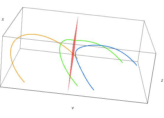
Figure 1: U-shaped profiles of the geodesics required to compute the two-point correlators. Gauge theory time runs horizontally to the right and is parametrized by the $v$-coordinate in eq. (1). The endpoints of the trajectories, located at the AdS boundary, are separated in space and time (see (44)). The geometry to the left of the shell is pure AdS ($\sf T=0$), at $v=0$ energy and charge are injected homogeneously into the system giving rise to the formation of a charged black hole geometry ($\sf T>0$) to the right of the shell. Early geodesics (orange) intersect the shell at $v=0$ (red plane) only once, late geodesics (green) intersect it twice, while thermalized geodesics (blue) do not intersect it at all.

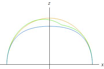
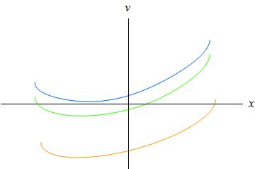
Figure 2: Plots of the three types of geodesics that we encounter in our calculations. Early geodesics (orange) intersect the shell at $v=0$ (red line) only once, late geodesics (green) intersect it twice, while thermalized geodesics (blue) do not intersect it at all. The plots show the $xz$ (left), the $xv$ (center) and $vz$ (right) projections.

We choose to parametrize the curve as $x^{\mu}(x)=(v(x),z(x),x_{1}(x)\!=\!x,{\bf x}_{d-2})$ with ${\bf x}_{d-2}$ constant, and without any loss of generality we take $x_{i}<x<x_{f}$, with $x_{i},x_{f}$ the extremes of the $\sf U$-shaped curve whose tip sits at $x=0$. The boundary conditions for the trajectories we are interested in are

$$z(x_{i})=z(x_{f})=z_{\epsilon},\quad\quad v(x_{i})=t_{i}\,,\quad\quad v(x_{f})=t_{f}\,.$$ (42)

where, as mentioned above, we have regularized the problem by considering geodesics whose endpoints lie at $z=z_{\epsilon}$, instead of $z=0$ ($z_{\epsilon}\to 0$ should be taken at the end of the computations). Alternatively, the trajectories can be characterized in terms of the boundary conditions at the tip

$$z(0)=z_{*},\quad\quad v(0)=v_{*}\,,\quad\quad v^{\prime}(0)=v^{\prime}_{*}\,,\quad\quad\quad z^{\prime}(0)=0\,.$$ (43)

Viewed from the tip, two branches appear: (i) for $x_{i}<x<0$ the trajectory describes $z\in(0,z_{*})$ and hence $z^{\prime}>0$, (ii) while for $0<x<x_{f}$ it goes from the tip $z=z_{*}>0$ to the boundary $z=0$ therefore $z^{\prime}<0$. These two branches correspond to the two signs in (48)

The space and time separation characterizing the geodesic are given by

$$\ell=x_{f}-x_{i}\,,\qquad\qquad\qquad\Delta t=t_{f}-t_{i}\,.$$ (44)

At this point we can already suspect that $\ell$ will be a growing function of $z_{*}$, implying that any upper cutoff in $z_{*}$ imposes an upper cutoff in $\ell$. This behavior is well known and can be explicitly checked in the numerical calculations of the forthcoming sections. Moreover, this implies that if we are interested in restricting the region of the geometry to be probed by our geodesics to the near boundary patch, then we must impose an upper bound on $\ell<\ell_{\sf Max}$. In other words, the violation of energy conditions in the bulk for the charging case imposes an IR cutoff in the degrees of freedom that can be probed (see fig. 3).

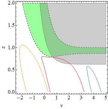
Figure 3: Geodesics and the null energy condition: the grey zone depicts the (IR) region in which the null energy condition (32) is violated. We also depict the position of the outer/inner horizon, defined as the $z(v)$ solution to $f(z,v)=0$, as dashed lines. The yellow and blue geodesics do not explore the sick region and can be used to analyze thermalization. The red geodesics on the other hand enter into the sick region and we cannot trust them to probe the thermalization process, in other words the background geometry can be used to analyze the thermalization of degrees of freedom above an IR cutoff. Note that in concordance with the discussion below (32), the region where the horizon recedes does not satisfy the energy conditions. The background interpolates between pure $AdS$ in the past to a $Q=2$ and $M=1+Q^{2}$ black hole in the future.

III.1 Equilibrium state

Inserting the eternal AdSRN solution (13) into the action (39) we get

$$S^{E}_{\sf equilibrium} = mL\int_{x_{i}}^{x_{f}}dx\left(\frac{1}{z}\sqrt{1-f\,v^{\prime 2}-2z^{\prime}v^{\prime}}-q_{E}(\gamma{Q}z^{d-2}-\mu)v^{\prime}\right)\,,$$ (45)

where prime $(^{\prime})$ denotes derivative with respect to the Euclidean parameter $\tau_{E}$, that we have gauge fixed to $\tau_{E}=x$. The first term corresponds to the geodesic length, while the second codifies the coupling to the gauge potential. Notice that only for the case of geodesics starting and ending at the same value of $v$ can one drop the $\mu$ contribution on the second term.

The two resulting second order equations of motion can be shown to have two first integrals: one coming from reparametrization invariance, which in our coordinates turns into the conserved Hamiltonian generating translation along the $x$ parameter, and the second from $v$-independence of the metric. The equations to be solved are

$$z\sqrt{1-f\,v^{\prime 2}-2z^{\prime}v^{\prime}} = \frac{1}{\tilde{E}}\,,$$ (46)

$$(f\,v^{\prime}+z^{\prime})\tilde{E}+\gamma q_{E}Qz^{d-2} = f_{*}\,v^{\prime}_{*}\tilde{E}+\gamma q_{E}Qz_{*}^{d-2}\,,$$ (47)

where the value of the constants on the right hand side have been fixed at the tip of the $\sf U$-shaped curve ($x=0$) according to the conditions (43): ${\tilde{E}}=1/z_{*}\sqrt{1-f_{*}\,v_{*}^{\prime 2}}$ where $f(z_{*})=f_{*}$.

Solving (46)-(47) for $z^{\prime}$ one obtains

$$z^{\prime}=\pm\sqrt{\left(\frac{1}{\tilde{E}^{2}z^{2}}-1\right)f+\left(f_{*}v^{\prime}_{*}+\frac{\gamma q_{E}Q}{\tilde{E}}(z_{*}^{d-2}-z^{d-2})\right)^{2}}\,.$$ (48)

As explained above, the double sign in this expression corresponds to the two branches of the U-shaped trajectory: the positive sign corresponds to $x_{i}<x<0$ while the negative one happens for $0<x<x_{f}$. Solving for $v^{\prime}$ one obtains

$$v^{\prime}=\frac{1}{f}\left(\frac{\gamma q_{E}Q}{\tilde{E}}(z_{*}^{d-2}-z^{d-2})+f_{*}\,v^{\prime}_{*}-z^{\prime}\right)\,,$$ (49)

with $z^{\prime}$ given by (48). The two parameters at the tip ($z_{*},v^{\prime}_{*}$) are related to ($\ell,\Delta t$) by noting that

$$\ell=x_{f}-x_{i}=\int_{x_{i}}^{0}dx+\int_{0}^{x_{f}}dx=2\int_{0}^{z_{*}}\frac{dz}{z^{\prime}}\,,$$ (50)

and

$$\Delta t=t_{f}-t_{i}=v(x_{f})-v(x_{i})=\int_{x_{i}}^{x_{f}}dx\,v^{\prime}\,.$$ (51)

Finally, inserting (46) and (49) into (45) we can express the on-shell action as

$$S^{E}_{\begin{subarray}{c}\!\!\!\!\sf on-shell\\ \sf equilibrium\end{subarray}}=2\frac{mL}{\tilde{E}}\int_{z_{\epsilon}}^{z_{*}}\frac{dz}{z^{\prime}}\left(\frac{1}{z^{2}}+\gamma q_{E}Q\frac{z^{d-2}}{f}\left(\gamma q_{E}Q(z^{d-2}-z_{*}^{d-2})-f_{*}v^{\prime}_{*}\tilde{E}\right)\right)+mL\,\mu q_{E}\Delta t\,.$$ (52)

Since the on-shell action diverges when the endpoints of the trajectory reach the boundary, we have regularized (52) by introducing a cutoff $z_{\epsilon}$. The factor of two arises from the two branches of the trajectory giving identical contributions. The formulae above enable us to compute the on shell action (52) as a function of $\ell$ and $\Delta t$. Notice that the $v$-independence of the background implies that no dependence on $v_{*}$ is expected.

III.2 Time dependent state

The action for a charged particle moving in the time dependent metric takes the form (45), but with the constants $Q$ and $M$ substituted by the $v$-dependent functions $\hat{Q}$ and $\hat{M}$.

$$S^{E}_{\sf t-dependent} = mL\int_{x_{i}}^{x_{f}}dx\left(\frac{1}{z}\sqrt{1-f\,v^{\prime 2}-2z^{\prime}v^{\prime}}-q_{E}(\gamma{\hat{Q}}z^{d-2}-\hat{\mu})v^{\prime}\right)\,.$$ (53)

Notice that we have also introduced a $v$-dependent $\hat{\mu}$ (see discussion below (34)). Due to the lack of $v$-translation invariance, the on shell action cannot be taken into a pure $z$ integral as in (52). The equations to be solved now are

$$z\sqrt{1-f\,v^{\prime 2}-2z^{\prime}v^{\prime}} = \frac{1}{E}\,,$$ (54)

$$E\left(fv^{\prime\prime}+z^{\prime\prime}+\frac{f_{v}v^{\prime 2}}{2}+f_{z}z^{\prime}v^{\prime}\right) = -\gamma{q_{E}}\hat{Q}(d-2)z^{d-3}z^{\prime}\,,$$ (55)

where the value of $E$ is again fixed at the tip of the curve (43) and given by ${E}=1/z_{*}\sqrt{1-f_{*}\,v_{*}^{\prime 2}}$.

These equations are solved numerically by the shooting method. In practice, we shoot from the turning point $z_{*}$ with initial (final) conditions (43) for $0<x<x_{f}$ and $x_{i}<x<0$. For each choice of values $(z_{*},v_{*},v^{\prime}_{*})$ at the tip we will find an $\sf U$-shaped geodesic characterized by $(\ell,\Delta t,t_{f})$ (see Figs. 1 and 2). The plots below give the thermalization curves for $\delta S$ given by (41) with the on-shell action (53) being generically a function $S^{E}_{\begin{subarray}{c}\!\!\!\!\!\!\!\!\!\!\sf on-shell\\ \sf t-dependent\end{subarray}}\!\!\!\!\!\!(\ell,\Delta t,t_{f})$.

Notice that, since the time dependent charging background violates the null energy conditions for large enough $z$, in such case we need to make sure that our geodesics are only probing the healthy part of the geometry (see Fig. 3). As mentioned before, this implies that we can probe thermalization with correlation functions with bounded $\ell<\ell_{\sf Max}$. On the other hand in the discharging background, we have no such IR cutoff and we can probe the thermalization with any value of $\ell$.

IV Results

The considerations of the previous sections were made for arbitrary functions $\hat{M}$ and $\hat{Q}$. In this section, in order to proceed with the numerical evaluation of the thermalization time for different probes, we will need explicit expressions for those functions. We choose

$$\hat{M} = \frac{M-M_{\sf in}}{2}\left(1+\tanh\left(\frac{v}{v_{0}}\right)\right)+M_{\sf in}\,,$$ (56)

$$\hat{Q} = \frac{Q-Q_{\sf in}}{2}\left(1+\tanh\left(\frac{v}{v_{0}}\right)\right)+Q_{\sf in}\,.$$ (57)

Here $v_{0}$ parametrizes the shell thickness and the $v_{0}\to 0$ case corresponds to the shock wave discussed in bala . These functions satisfy

$${\lim_{v\to{-\infty}}}\hat{M}=M_{\sf in}\,,\qquad\qquad\qquad{\lim_{v\to\infty}}\hat{M}=M$$

$${\lim_{v\to{-\infty}}}\hat{Q}=Q_{\sf in}\,,\qquad\qquad\qquad\;\;{\lim_{v\to\infty}}\hat{Q}=Q\,.$$ (58)

Therefore the backgrounds we consider interpolate between an AdSRN black hole with mass $M_{\sf in}$ and charge $Q_{\sf in}$ in the distant past $v\ll v_{0}$ and an AdSRN black hole with mass $M$ and charge $Q$ in the distant future $v\gg v_{0}$.

IV.1 Vanishing background charge

We start by analyzing the thermalization process in the case of vanishing background charge, which corresponds to a thermal quench with vanishing chemical potential in the boundary theory. To this end, we choose

$$\hat{M} = \frac{M-M_{\sf in}}{2}\left(1+\tanh\left(\frac{v}{v_{0}}\right)\right)+M_{\sf in}\,,$$ (59)

$$\hat{Q} = 0\,.$$ (60)

For the case of vanishing $\Delta t$ we reproduced the results of bala , and for nonvanishing $\Delta t$ we find results in agreement to those in Aparicio:2011zy .

The results are summarized in Fig. 4, where the thermalization curves $\delta S$ involving the on-shell action are plotted as functions of $t_{f}$. The thermalization time, defined as the approximated value of $t_{f}$ at which the curve reaches the horizontal axis $\delta S=0$, increases with $\ell$ and with $\Delta t$, implying that UV degrees of freedom thermalize first. This is the phenomenon known as “top down thermalization”. Moreover, we see that the thermalization time also increases with the dimension of the system.

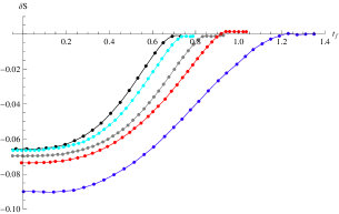
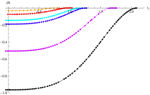
Figure 4: Two point correlators as a function of $t_{f}$ for a thermal quench in the absence of chemical potential (Sect IV.A).   Left: plots for $d=3$, $\ell=1.4$ and $\Delta t=0,0.1,0.3,0.5,1$ (black, azure, gray, red and blue resp.).   Center: plot for $d=3$, $\Delta t=0.5$ and $\ell=1,1.4,1.8,2,3,4$ (orange, red, azure, blue, violet and black resp.).   Right: plot for $\ell=1.4$, $\Delta t=0.5$ and $d=3,4,5$ (red, blue and violet resp.). All cases correspond to a chargeless background interpolating between $M_{\sf in}=0$ and $M=1$.

IV.2 Vanishing probe charge

We now consider a quench in both the temperature and the chemical potential. We first study the effects of the background on a vanishing probe charge $q_{E}=0$. For the sake of illustration, we set our background to be pure AdS (${\sf T}=\mu=0$) in the asymptotic past, and AdSRN (${\sf T},\mu\neq 0$) in the asymptotic future, namely

$$\hat{M} = \frac{M}{2}\left(1+\tanh\left(\frac{v}{v_{0}}\right)\right)\,,$$ (61)

$$\hat{Q} = \frac{Q}{2}\left(1+\tanh\left(\frac{v}{v_{0}}\right)\right)\,.$$ (62)

As could have been expected, since we are probing the system with uncharged operators ($q_{E}=0$), the background charge $\hat{Q}$ has little effect in the form of the thermalization curves. The phenomenon of top-down thermalization is again present, and the thermalization time grows with the dimension of the field theory as in the previous case. The results are depicted in Fig. 5 and are in agreement with those of Refs. martin .

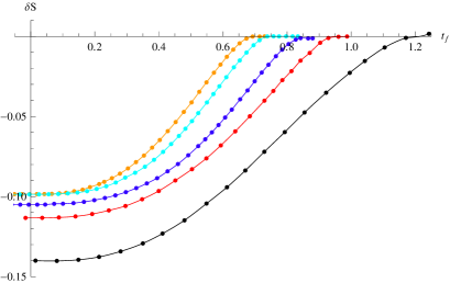
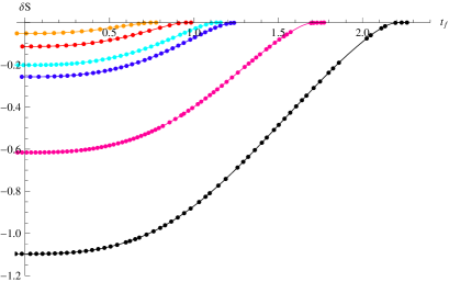
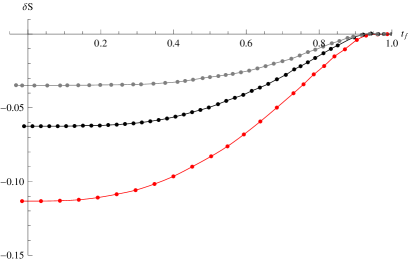
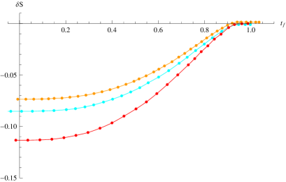
Figure 5: Two point functions for uncharged operators as a function of $t_{f}$ for a an energy and charge quench (Sect IV.B). Top left: plots for $d=3$, $\ell=1.4$ and $\Delta t=0,0.1,0.3,0.5,1$ (orange, azure,blue, red and black resp.). Top right: plots for $d=3$, $\Delta t=0.5$, and $\ell=1,1.4,1.8,2,3,4$ (orange, red, azure, blue, violet and black resp.). Bottom left: plots for $\ell=1.4$, $\Delta t=0.5$ and $d=3,4,5$ (red, black and grey resp.). Bottom right: plots for $d=3$, $\ell=1.4$, $\Delta t=0.5$ and $Q=0,0.5,1$ (orange, azure and red resp.). In all cases we start from pure AdS at past infinity to $M=1$ at future infinity, for the first three cases the final charge is $Q=1$.

IV.3 Constant background charge

To analyze the thermalization process for a thermal and chemical potential quench we consider the $\hat{M}$ and $\hat{Q}$ functions to be

$$\hat{M} = \frac{M-M_{\sf in}}{2}\left(1+\tanh\left(\frac{v}{v_{0}}\right)\right)+M_{\sf in}\,,$$ (63)

$$\hat{Q} = Q_{\sf in}\,.$$ (64)

This background interpolates between a AdSRN black hole of mass $M_{\sf in}$ and charge $Q_{\sf in}$ in the distant past $v\ll v_{0}$, to a heavier AdSRN black hole ($M>M_{\sf in}$) in the distant future $v\gg v_{0}$ preserving the charge $Q_{\sf in}$. In the following we choose to re-scale the $z$-coordinate so as to have $M_{\sf in}=1+Q_{\sf in}^{2}$ in the far past. This ensures that the background satisfies the bound (9) in the past, and since the evolution increases the mass while keeping the charge constant, (32) is also satisfied. Notice that although the background charge is constant, the chemical potential changes when injecting energy into the system. The reason for this is that we should demand regularity of the euclidean rotated asymptotic geometries (see discussion after eq. (34)). We choose the profile for the chemical potential to be

$$\hat{\mu}=\frac{\mu-\mu_{\sf in}}{2}\left(1+\tanh\left(\frac{v}{v_{0}}\right)\right)+\mu_{\sf in}\,,$$ (65)

with

$$\mu_{\sf in}=\gamma Q_{{\sf in}},\quad\quad\mu=\gamma Q_{{\sf in}}z_{h}^{d-2}\,,$$ (66)

where $z_{h}<1$ is the horizon position after the quench. The initial position being $z_{\sf in}=1$ due to the condition $M_{\sf in}=1+Q_{\sf in}^{2}$. Notice that during the quench the absolute value of the chemical potential reduces, but it cannot reach $\mu=0$.

Figs. 6 to 9 show the results corresponding to an interpolation between $M_{\sf in}=2$ and $M=3$ with $Q_{\sf in}=1$. In Figs. 6 and 7 we see that thermalization time increases as a function of $\ell$ and $\Delta t$ respectively, showing again the top-down thermalization effect, and Fig. 8 shows that the thermalization time increases with the spacetime dimension. Finally in Fig. 9 we see that, for positive chemical potential, the thermalization time probed with charged operators grows with the charge $q_{E}$ of the operator, this is an expected result from the gauge theory perspective.

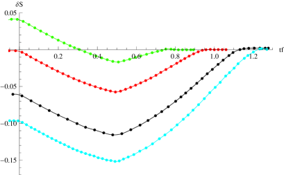
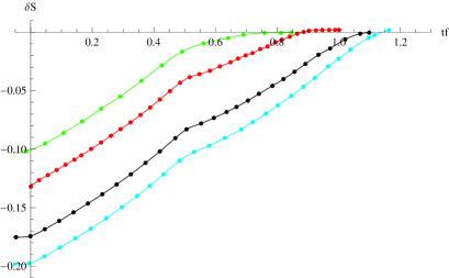
Figure 6: Two point functions of charged operators as a function of $t_{f}$ for a thermal and chemical potential quench modeled by an interpolation between $M_{\sf in}=1+Q_{\sf in}^{2}$ in the far past to $M=3$ in the future, keeping the charge $Q=Q_{\sf in}=1$ constant (Sect IV.C). The plots correspond to $d=3$, $\Delta t=0.5$ and $\ell=1,1.4,1.8,2$ (green, red, black and azure resp.).
Left: $q_{E}=1$. Right: $q_{E}=-1$.

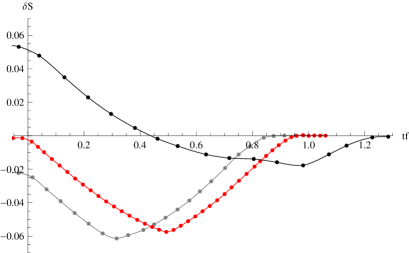
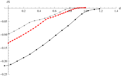
Figure 7: Two point functions of charged operators as a function of $t_{f}$ for a thermal and chemical potential quench modeled by an interpolation between $M_{\sf in}=1+Q_{\sf in}^{2}$ in the far past to $M=3$ in the future, keeping the charge $Q=Q_{\sf in}=1$ constant (Sect IV.C). The plots correspond to $d=3$, $\ell=1.4$ and $\Delta t=0.3,0.5,1$ (gray, red and black resp.). Left: $q_{E}=1$. Right: $q_{E}=-1$.

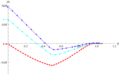
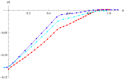
Figure 8: Two point functions of charged operators as a function of $t_{f}$ for a thermal and chemical potential quench modeled by an interpolation between $M_{\sf in}=1+Q_{\sf in}^{2}$ in the far past to $M=3$ in the future, keeping the charge $Q=Q_{\sf in}=1$ constant (Sect IV.C). The plots correspond to $\ell=1.4$, $\Delta t=0.5$ and $d=3,4,5$ (red, azure, blue resp.). Left: $q_{E}=1$. Right: $q_{E}=-1$.

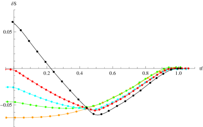
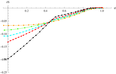
Figure 9: Two point functions of charged operators as a function of $t_{f}$ for a thermal and chemical potential quench modeled by an interpolation between $M_{\sf in}=1+Q_{\sf in}^{2}$ in the far past to $M=3$ in the future, keeping the charge $Q=Q_{\sf in}=1$ constant (Sect IV.C). The plots correspond to $d=3$, $\ell=1.4$, $\Delta t=0.5$ and $|q_{E}|=0,0.3,0.65,1,2$ (yellow, green, azure, red and black resp.). Left: $q_{E}>0$. Right: $q_{E}<0$.

A peculiar feature appears in all the figures: a peak arises at fixed $t_{f}$ where the derivative of $\delta S$ with respect to $t_{f}$ has a sudden change. This can be understood with the help of Fig. 7, in which it is evident that such peak happens for $t_{f}\simeq\Delta t$. Indeed, each point $t_{f}$ in the curves represents a geodesic that, according to our boundary conditions (42), starts at the boundary at $t=t_{f}-\Delta t$ and ends at $t=t_{f}>0$. Since the shell enters space at $t=0$, early trajectories starting at negative times ($t_{f}<\Delta t$) cross the shell once in order to return to the boundary. On the other hand, late trajectories starting at positive times ($t_{f}>\Delta t$) either cross the shell twice, or do not cross it at all, this last case corresponds to a thermalized situation (see Fig.1). These three classes of trajectories prove the spacetime in different ways. Let us first assume $\hat{Q}q_{E}>0$, then, for early trajectories, the gravitational force of the background competes with the electromagnetic interaction during the first part of the trajectory (close to $t=t_{f}-\Delta t$), after the particle crosses the shell the two forces pull in the same direction (close to $t=t_{f}$). For late trajectories, the two forces compete only close to the tip of the trajectory, and cooperate at both extremes, close to $t=t_{f}-\Delta t$ and $t=t_{f}$. Finally in the third case the forces cooperate all along the trajectory. The same reasoning can be repeated for $\hat{Q}q_{E}<0$, with the regions in which the forces compete or cooperate being interchanged. This can be visualized in Figs. 1 and 2, in which the three types of geodesics are shown. The absence of peaks for vanishing probe charge is another evidence of their relation to the electromagnetic interaction.

As can be seen in Fig. 9, there is a remarkable additional feature on the plots: there exists a value of $t_{f}$ such that the function $\delta S$ does not depend on the probe charge $q_{E}$. We do not have an explanation for this behavior at the moment.

IV.4 Discharging background

To study a discharging background of the kind described in section II.2 we need to choose $|Q|<|Q_{\sf in}|$. For illustrative purposes we will take the extreme case $Q=0$ with the functions $\hat{M}$ and $\hat{Q}$ reading

$$\hat{M} = \frac{M-M_{\sf in}}{2}\left(1+\tanh\left(\frac{v}{v_{0}}\right)\right)+M_{\sf in}\,,$$ (67)

$$\hat{Q} = -\frac{Q_{\sf in}}{2}\left(1+\tanh\left(\frac{v}{v_{0}}\right)\right)+Q_{\sf in}\,.$$ (68)

These functions interpolate between an AdSRN black hole with mass $M_{\sf in}$ and charge $Q_{\sf in}$ in the distant past $v\ll v_{0}$ and an AdS black hole with mass $M$ (and vanishing charge) in the distant future $v\gg v_{0}$. We again re-scale the radial coordinate so that $M_{\sf in}=1+Q_{\sf in}^{2}$ in the initial state. In the final state, the bound (9) is satisfied since the charge vanishes. From the dual point of view, we are modeling the process of a sudden decrease of the absolute value of the chemical potential while energy is being injected into the system. We would like to mention that this instance cannot be modeled with a constant charge background and complements the results of the previous section.

Results are shown in Figs. 10 to 13. Again we see that top-down thermalization arises and that the thermalization time grows with $\ell$, $\Delta t$ and the space dimension. The peak at $t_{f}=\Delta t$ is also present, the reasons being the same as explained in the previous section. Thermalization time also increases with the charge of the probe.

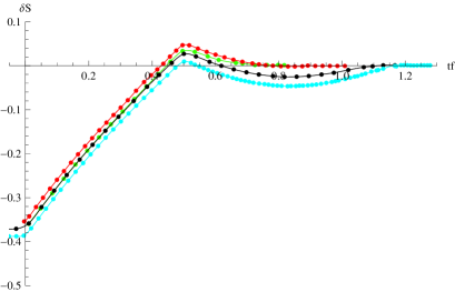
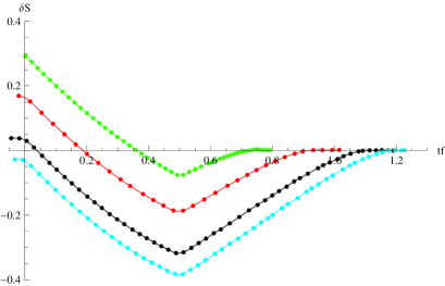
Figure 10: Two point functions of charged operators as a function of $t_{f}$ for a thermal and chemical potential quench leading to a final vanishing chemical potential (Sect IV.D). Plots correspond to $d=3$, $\Delta t=0.5$ and $\ell=1,1.4,1.8,2$ ( green, red, black and azure resp.). Left: $q_{E}=1$. Right: $q_{E}=-1$. In Figs. 10-14, the geometry interpolates between a RNAdS with $M_{\sf in}=1+Q_{\sf in}^{2}$, $Q_{\sf in}=-1$ and pure AdS with $M=3$.

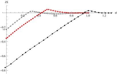
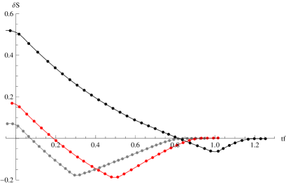
Figure 11: Two point functions of charged operators as a function of $t_{f}$ for a thermal and chemical potential quench leading to a final vanishing chemical potential (Sect IV.D). Plots correspond to $d=3$, $\ell=1.4$ and $\Delta t=0.3,0.5,1$ (gray, red and black resp.). Left: $q_{E}=1$. Right: $q_{E}=-1$.

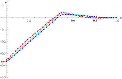
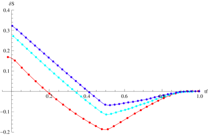
Figure 12: Two point functions of charged operators as a function of $t_{f}$ for a thermal and chemical potential quench leading to a final vanishing chemical potential (Sect IV.D). Plots correspond to $\ell=1.4$, $\Delta t=0.5$ and $d=3,4,5$ (red, azure and blue resp.). Left: $q_{E}=1$. Right: $q_{E}=-1$.

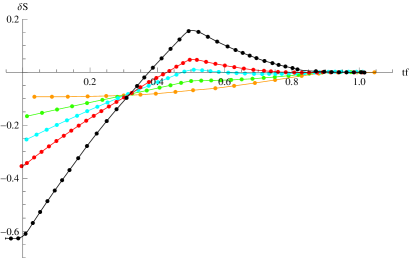
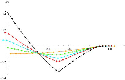
Figure 13: Two point functions of charged operators as a function of $t_{f}$ for a thermal and chemical potential quench leading to a final vanishing chemical potential (Sect IV.D). Plots correspond to $d=3$, $\ell=1.4$, $\Delta t=0.5$ and $|q_{E}|=0,0.3,0.65,1,2$ (orange, green, azure, red and black resp.). Left: $q_{E}>0$. Right: $q_{E}<0$.

IV.5 Charging background

We conclude by analyzing the thermalization process for a quench leading to an increase on both the temperature and the chemical potential (this situation has been considered before in martin for the case of uncharged operators). The functions $\hat{M}$ and $\hat{Q}$ read

$$\hat{M} = \frac{M}{2}\left(1+\tanh\left(\frac{v}{v_{0}}\right)\right)\,,$$ (69)

$$\hat{Q} = \frac{Q}{2}\left(1+\tanh\left(\frac{v}{v_{0}}\right)\right)\,.$$ (70)

These functions interpolate between a pure AdS solution in the distant past $v\ll v_{0}$, to a AdSRN solution in the distant future $v\gg v_{0}$ with mass $M$ and charge $Q$. We rescale the radial coordinates so as to have $M=1+Q^{2}$ in the future state. From the dual point of view, as energy flows into the system, the absolute value of the chemical potential suddenly increases. As discussed in Sect II.2, in the present situation the null energy condition is violated in the deep IR, so we must check that our geodesics do not reach such region (see Fig. 3).

Results are shown in Figs. 14 to 17, with features similar to the previous cases, namely, top-down thermalization, thermalization time growing with the dimension of space, peaks denoting the transition between the different classes of geodesics, etc. It is worth mentioning that the swallow tale structure found in martin also appears for non-vanishing probe charges as can be seen in Fig. 18.

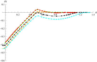
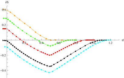
Figure 14: Two point functions of charged operators as a function of $t_{f}$ for a thermal and chemical potential quench modeled by a charging background (Sect. IV.E). Plots corresponding to $d=3$, $\Delta t=0.5$ and $\ell=1,1.4,1.8,2$ (orange, green, red, black and azure resp.). Left: $q_{E}=1$. Right: $q_{E}=-1$.
The geometry interpolates between pure AdS and AdSRN with $M=1+Q^{2}$ and $Q=1$.

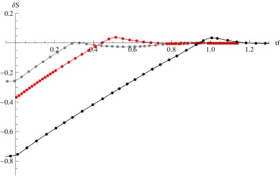
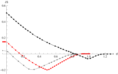
Figure 15: Two point functions of charged operators as a function of $t_{f}$ for a thermal and chemical potential quench modeled by a charging background (Sect. IV.E). Plots corresponding to $d=3$, $\ell=1.4$ and $\Delta t=0.3,0.5,1$ (gray, red and black resp.).
Left: $q_{E}=1$. Right: $q_{E}=-1$.

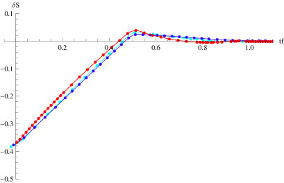
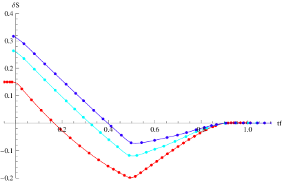
Figure 16: Two point functions of charged operators as a function of $t_{f}$ for a thermal and chemical potential quench modeled by a charging background (Sect. IV.E). Plots corresponding to $d=3$, $\ell=1.4$ and $\Delta t=0.5$ for $d=3,4,5$ (red, azure and blue resp.). Left: $q_{E}=1$. Right: $q_{E}=-1$.

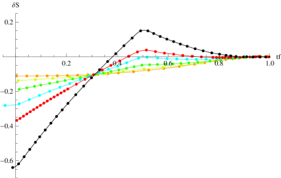
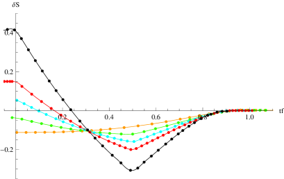
Figure 17: Two point functions of charged operators as a function of $t_{f}$ for a thermal and chemical potential quench modeled by a charging background (Sect. IV.E). Plots corresponding to $d=3$, $\ell=1.4$ and $\Delta t=0.5$. Left: $q_{E}=0,0.1,0.3,0.65,1,2$ (orange, light yellow, green, azure, red, black resp.) Right: $-q_{E}=0,0.3,0.65,1,2$ (orange, green, azure, red and black resp.).

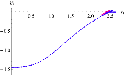
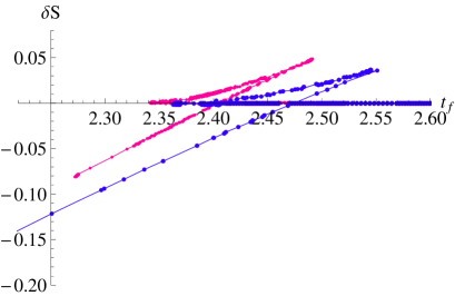
Figure 18: Two point functions of charged operators as a function of $t_{f}$ for a thermal and chemical potential quench modeled by a charging background (Sect. IV.E). Plots corresponding to a charging backgound from pure AdS to an extremal AdSRN. Plots coreespond to $d=3$, $M=1+Q^{2}$, $Q=\sqrt{3}$, $\ell=4$, $\Delta t=0.5$ and $q_{E}=0,0.5$ (blue and violet resp.). On the right we have zoomed the swallow tale region.

V Conclusions

We have analyzed the energy conditions for the external matter needed to support a family of charged AdS-Vaidya metrics. The metrics studied interpolate between two AdSRN black holes with different mass and charge, or between pure AdS and an AdSRN black hole with non-vanishing charge. They have been used in the literature, via the AdS/CFT correspondence, to model the thermalization process in a strongly coupled plasma after a quench in energy and chemical potential.

We found that the null energy condition is violated in the infrared region of the geometry for increasing mass whenever the absolute value of the black hole charge increases in time. On the other hand, when the absolute value of the black hole charge is kept constant or decreases, the null energy condition is satisfied everywhere. This implies that charged Vaidya metrics can be used to analyze thermalization processes for all energy scales only when the quench decreases the absolute value of the chemical potential. On the other hand, when the quench increases the absolute value of the chemical potential, then the metric is only useful for probing the thermalization process above an IR cutoff1.

We applied the above results to study the thermalization of a strongly coupled plasma after a quench in the energy and chemical potential, considering the cases where the chemical potential either increases or decreases in absolute value. As probe of thermalization we considered charged operators two point functions. We found that the thermalization time increases with the charge of the operator, as well as with the dimension of the field theory. As expected in these kind of holographic constructions, the thermalization is top-down, in the sense that UV degrees of freedom thermalize earlier, followed by IR ones.

VI Acknowledgments

We thank Martin Schvellinger, Walter Baron and Damian Galante for helpful discussions on thermalization of strongly coupled plasmas via AdS/CFT. We also thank Anibal Iucci and Nicolás Nessi for helpful exchange on the general knowledge about thermalization after quenches and Jerónimo Peralta Ramos and Pablo Rodriguez Ponte for discussions. This work was partially supported by Conicet grant PIP2009-0396, PIP 0595/13, ANPCyT grant PICT2008-1426 and UNLP grant 11/X648.

Appendix A Eddington-Finkelstein null coordinates

For completeness we quote here some well known facts of the Eddington-Finkelstein coordinate system $X^{\mu}=(v,{\bf x},z)$ chosen in (1). Parametrizing the geodesics as $X^{\mu}=(v(z),{\bf x}(z),z)$ it is immediate to see that the curve $X^{\mu}=(v_{0},{\bf x}_{0},z)$ moving along the holographic direction is null. In what follows we show that the sign of the $dvdz$ term in (1) determines whether the curve is either ingoing or outgoing. This in turn determines whether the mass shell in a Vaydia metric is ingoing or outgoing.

We start by considering the timelike vector $\partial_{v}$ to be future directed. The null geodesics on the $(v,z)$ plane for the AdS_d+1 black hole geometry are obtained from

$$(1-Mz^{d})dv^{2}\pm 2dvdz=0\Longrightarrow v(z)=C\mp 2z\,_{2}F_{1}\left(1,\frac{1}{d},1+\frac{1}{d},Mz^{d}\right)\,,$$ (71)

here $C$ is an integration constant and ${}_{2}F_{1}$ is Gauss hyper-geometric function, blowing up at $Mz^{d}=1$ and having an expansion ${}_{2}F_{1}\approx z+{\cal O}(z^{d+1})$ near the boundary of AdS. The upper sign choice in (71) therefore implies that the geodesic displayed in (71) is escaping from the horizon as $v$ increases. Taking into account that $\partial_{v}$ is timelike outside the horizon, we conclude that the $v=v_{0}$ curve corresponds to a radially ingoing null geodesic.

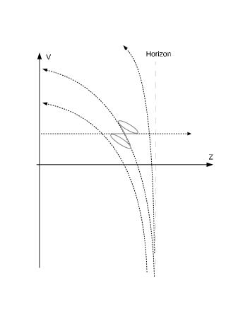
Figure 19: Null geodesics and light cones for the EF (ingoing) coordinates chosen in the body of the paper. The plot shows the solutions of (71) for the upper sign.

Appendix B World line formalism and geodesic approximation

The bulk propagator $G(x_{2}^{\alpha},z_{2}|\,x_{1}^{\alpha},z_{1})$ in (35) is the Green function of the equation of motion of a bulk charged scalar field, or in other words

$$G(x_{2}^{\alpha},z_{2}|\,x_{1}^{\alpha},z_{1}) = \left\langle{x_{2}^{\alpha},z_{2}}\left|\,\frac{i}{g^{\mu\nu}D_{\mu}D_{\nu}-m^{2}+i\epsilon}\,\right|{x_{1}^{\alpha},z_{1}}\right\rangle\,,$$ (72)

where $D_{\mu}=\partial_{\mu}-i{\sf e}A_{\mu}$ is the covariant derivative for a charged scalar of charge ${\sf e}$. Schwinger’s proper time representation consists in rewriting the inverse operator (72) as bastianelli ; Marolf ; kiri

$$G(x_{2}^{\alpha},z_{2}|\,x_{1}^{\alpha},z_{1}) = \int_{0}^{\infty}dT\left\langle{x_{2}^{\alpha},z_{2}}\left|\,e^{iT\left(g^{\mu\nu}D_{\mu}D_{\nu}-m^{2}+i\epsilon\right)}\,\right|{x_{1}^{\alpha},z_{1}}\right\rangle\,.$$ (73)

The exponential inside the bracket can be understood as the evolution operator for the Hamiltonian $H=-g^{\mu\nu}D_{\mu}D_{\nu}+m^{2}$, which allows us to write

$$G({x_{2}^{\alpha},z_{2}|\,x_{1}^{\alpha},z_{1}})=\int_{0}^{\infty}dT\int_{x(0)=(x_{1}^{\alpha},z_{1})}^{x^{\mu}(T)=(x_{1}^{\alpha},z_{1})}\!\!\!\!{\cal D}x(\tau)\,e^{iS_{\sf 1particle}[x(\tau)]}\,,$$

$$\mbox{with}\qquad S_{\sf 1particle}[x(\tau)]=\int_{0}^{T}d\tau\left(\frac{1}{4}g_{\mu\nu}\dot{x}^{\mu}\dot{x}^{\nu}+{\sf e}A_{\mu}\dot{x}^{\mu}-m^{2}\right)\,.$$ (74)

Here $S_{\sf 1particle}[x(\tau)]$ is a one-particle action written in terms of a world line proper time parameter $\tau\in[0\dots T]$, and a dot ($\dot{~}{}$) means derivative with respect to $\tau$. We can rescale $\tau\to\tau T$ in order to get $\tau\in[0\dots 1]$ and we end up with

$$G({x_{2}^{\alpha},z_{2}|\,x_{1}^{\alpha},z_{1}})=\int_{0}^{\infty}dT\int_{x^{\mu}(0)=(x_{1}^{\alpha},z_{1})}^{x^{\mu}(1)=(x_{2}^{\alpha},z_{2})}\!\!\!\!{\cal D}x(\tau)\,e^{iS_{\sf 1particle}[x(\tau)]}\,,$$

$$\mbox{with}\qquad S_{\sf 1particle}[x(\tau)]=\int_{0}^{1}d\tau\left(\frac{1}{4T}g_{\mu\nu}\dot{x}^{\mu}\dot{x}^{\nu}+{\sf e}A_{\mu}\dot{x}^{\mu}-Tm^{2}\right)\,.$$ (75)

Notice that this one-particle action is not invariant under reparametrization of the world line. Introducing the einbein $e_{\tau}(\tau)$, we can interpret (75) as a gauge fixed expression for an originally reparametrization invariant action Marolf ; kiri

$$G({x_{2}^{\alpha},z_{2}|\,x_{1}^{\alpha},z_{1}})=\int{\cal D}e_{\tau}(\tau)\delta({\dot{e}_{\tau}})\int_{x^{\mu}_{\sf initial}=(x_{1}^{\alpha},z_{1})}^{x^{\mu}_{\sf final}=(x_{2}^{\alpha},z_{2})}\!\!\!\!{\cal D}x(\tau)\,e^{iS_{\sf invariant}[x(\tau)]}\,,$$

$$\mbox{with}\qquad S_{\sf invariant}[x(\tau)]=\int d\tau\left(\frac{1}{4e_{\tau}}g_{\mu\nu}\dot{x}^{\mu}\dot{x}^{\nu}+{\sf e}A_{\mu}\dot{x}^{\mu}-e_{\tau}m^{2}\right)\,.$$ (76)

The gauge fixing amounts to setting $e_{\tau}=T$, and the $T$ integral in (75) corresponds to the leftover (Teichmüller) parameter after gauge fixing kiri . In the limit of large mass $m$, in which we are interested, we can take the semiclassical approximation of the integral (76), to have

$$G({x_{2}^{\alpha},z_{2}|\,x_{1}^{\alpha},z_{1}})=e^{iS_{\sf on-shell}(x^{\alpha}_{1},z_{1};x^{\alpha}_{2},z_{2})}\,,$$

$$\mbox{with}\qquad S_{\sf on-shell}({x_{1}^{\alpha},z_{1}|\,x_{2}^{\alpha},z_{2}})=\left.\int d\tau\left(-m\sqrt{-g_{\mu\nu}\dot{x}^{\mu}\dot{x}^{\nu}}+{\sf e}A_{\mu}\dot{x}^{\mu}\right)\right|_{x^{\mu}(\tau)=x^{\mu}_{\sf classical}(\tau)}\,,$$ (77)

where the quotient ${\sf e}/m$ is assumed finite in the large $m$ limit, and $x^{\mu}_{\sf classical}(\tau)$ are the classical trajectories starting at $(x^{\alpha}_{1},z_{1})$ and ending at $(x_{2}^{\alpha},z_{2})$.

Appendix C Accessing the classically forbidden region

The classical trajectories we need to compute lie completely in the classically forbidden region. Indeed, from the action

$$S=\int d\tau\left(-m\sqrt{-g_{\mu\nu}\dot{x}^{\mu}\dot{x}^{\nu}}+{\sf e}A_{\mu}\dot{x}^{\mu}\right)\,,$$ (78)

we find the canonical momenta

$$p_{\mu}=\frac{m\,g_{\mu\nu}\dot{x}^{\nu}}{\sqrt{-g_{\mu\nu}\dot{x}^{\mu}\dot{x}^{\nu}}}+{\sf e}A_{\mu}\,,$$ (79)

and time reparametrization invariance imply

$$g^{\mu\nu}(p_{\mu}-{\sf e}A_{\mu})(p_{\nu}-{\sf e}A_{\nu})+m^{2}=0\,,$$ (80)

As we now show, these momenta become imaginary in the near boundary region, implying that such region is forbidden from a classical point of view.

C.1 Vanishing probe charge

Let us first consider the case ${\sf e}=0$. Using the explicit form of our metric and gauge fields, the action reads

$$S=-mL\int d\tau\,\frac{1}{z}\sqrt{-\dot{\bf x}_{d-1}^{2}+f\dot{v}^{2}+2\dot{z}\dot{v}}\,.$$ (81)

The resulting canonical momenta are

$$p_{v} = -\frac{mL}{zR}(f\dot{v}+\dot{z})\,,$$

$$p_{z} = -\frac{mL}{zR}\dot{v}\,,\qquad\qquad\qquad\qquad{\rm with}\quad R=\sqrt{-\dot{\bf x}_{d-1}^{2}+f\dot{v}^{2}+2\dot{z}\dot{v}}\,,$$

$${\bf p}_{d-1} = \frac{mL}{zR}\dot{\bf x}_{d-1}\,,$$ (82)

and the constraint (80) results

$$fp_{z}^{2}-2p_{v}p_{z}+{\bf p}^{2}_{d-1}=-\frac{m^{2}L^{2}}{z^{2}}\,.$$ (83)

Since for small $z$ we have $f\simeq 1$, any $v$-dependence in $f$ is washed out near the boundary implying that the quantity $p_{v}$ becomes constant. For fixed $p_{v}$, the quadratic polynomial in $p_{z}$ in the left hand side of (83) has a lower bound at $p_{z}=p_{v}$. On the other hand, the right hand side becomes arbitrarily negative as $z\to 0$. Thus, for $z$ small enough, the relation cannot be satisfied with real momenta, and the momenta must become complex. Indeed, for small enough $z$ the relation (83) can be solved as $p_{z}\approx imL/z+p_{v}$, implying that it can be satisfied with pure imaginary momenta $p_{z}=ip_{z}^{E}$ and $p_{v}=ip_{v}^{E}$. Based on this, for generic $z$ we propose the ansatz ${\bf p}_{d-1}=i{\bf p}_{d-1}^{E}$, $p_{z}=ip_{z}^{E}$ and $p_{v}=ip_{v}^{E}$, and in this new variables we have

$$p_{v}^{E} = i\frac{mL}{zR}(f\dot{v}+\dot{z})\,,$$

$$p_{z}^{E} = i\frac{mL}{zR}\dot{v}\,,\qquad\qquad\qquad\qquad{\rm with}\quad R=\sqrt{-\dot{\bf x}_{d-1}^{2}+f\dot{v}^{2}+2\dot{z}\dot{v}}\,,$$

$${\bf p}^{E}_{d-1} = -i\frac{mL}{zR}\dot{\bf x}_{d-1}\,,$$ (84)

and

$$-f{p^{E}_{z}}^{2}+2p^{E}_{v}p^{E}_{z}-{{\bf p}^{E}_{d-1}}^{\!\!\!\!2}=-\frac{m^{2}L^{2}}{z^{2}}\,.$$ (85)

We can re-absorb the $i$ factors in the velocities via a Wick rotation of the wordline time $\tau=-i\tau_{E}$ obtaining

$$p_{v}^{E} = -\frac{mL}{zR}(fv^{\prime}+z^{\prime})\,,$$

$$p_{z}^{E} = -\frac{mL}{zR}v^{\prime}\,,\qquad\qquad\qquad\qquad{\rm with}\quad R=\sqrt{{\bf x}_{d-1}^{\prime 2}-fv^{\prime 2}-2z^{\prime}v^{\prime}}\,,$$

$${\bf p}^{E}_{d-1} = \frac{mL}{zR}{\bf x}^{\prime}_{d-1}\,,$$ (86)

where a prime $(^{\prime})$ means derivative with respect to $\tau_{E}$. With these redefinitions, the momenta (86) can be re-interpreted as derived from the Euclidean action obtained via the substitution $\tau=-i\tau_{E}$ in (81), namely

$$S_{E}=mL\int d\tau_{E}\,\frac{1}{z}\sqrt{{{\bf x}^{\prime}}_{d-1}^{2}-fv^{\prime 2}-2z^{\prime}v^{\prime}}\,.$$ (87)

In other words, the imaginary momenta of (81) in the forbidden region can be re-interpreted as the real momenta of its “Euclidean worldline time” version (87).

This “Euclideanization” implies re-interpreting the complex valued classical solution of the equations of motion in the classically forbidden region, as the real valued classical solution of the Wick rotated system. Notice that in solving relation (83) for small enough $z$ we could include a real part on the momenta $p_{z}=ip_{z}^{E}+p_{Re}$ and $p_{v}=ip_{v}^{E}-p_{Re}$, or for generic $z$ we could put ${\bf p}_{d-1}=i{\bf p}_{d-1}^{E}+{\bf p}_{Re}$, $p_{z}=ip_{z}^{E}+p_{Re}$ and $p_{v}=ip_{v}^{E}-p_{Re}$, what would be a more general solution. Nevertheless, with this complex momenta, the imaginary unit $i$ could not be removed from the equations of motion by Wick rotation of the worldline parameter $\tau=-i\tau_{E}$, and the there would be no real-valued Euclidean variables to access the forbidden region. As expexcted the square root $R$ in (86) is real only for spacelike trajectories. In other words, our Euclidean action (87) allows us to find trajectories joining spacelike separated boundary points.

The conclusion is that, in the absence of charge, spacelike separated points in the forbidden region can be joined by real classical trajectories of the Euclidean worldline time action (87), obtained from the original one (81) via the Wick rotation $\tau=-i\tau_{E}$. This is a standard prescription and the one used in bala .

C.2 Non-vanishing probe charge

C.2.1 Wick rotation of the worldline time and the probe charge

For non-vanishing charge on the other hand, several complications arise. In this case, the action read

$$S=\int d\tau\left(-\frac{mL}{z}\sqrt{-\dot{\bf x}_{d-1}^{2}+f\dot{v}^{2}+2\dot{z}\dot{v}}+{\sf e}A_{v}\dot{v}\right)\,.$$ (88)

Writing the momenta (79) explicitly we have

$$p_{v} = -\frac{mL}{zR}(f\dot{v}+\dot{z})+{\sf e}A_{v}\,,$$

$$p_{z} = -\frac{mL}{zR}\dot{v}\,,\qquad\qquad\qquad\qquad{\rm with}\quad\left\{\begin{array}[]{l}A_{v}=-{L\gamma\hat{Q}}z^{d-2}+\mu L\,,\\ {}\\ R=\sqrt{-\dot{\bf x}_{d-1}^{2}+f\,\dot{v}^{2}+2\dot{z}\dot{v}}\,,\end{array}\right.$$ (92)

$${\bf p}_{d-1} = \frac{mL}{zR}\dot{\bf x}_{d-1}\,,$$ (93)

while the relation (80) becomes

$$fp_{z}^{2}-2(p_{v}-{\sf e}A_{v})p_{z}+{\bf p}^{2}_{d-1}=-\frac{m^{2}L^{2}}{z^{2}}\,.\,.$$ (94)

Again close enough to the boundary the explicit $v$ dependence disappears, and the momentum $p_{v}$ becomes a constant. For fixed $p_{v}$ the polynomial in $p_{z}$ in the left hand side of (94) has a minimum at $p_{z}=p_{v}-{\sf e}\mu L$ while its right hand side becomes arbitrarily negative, implying that the relation cannot be satisfied for real momenta at small $z$. As in the previous case, this can be solved by pure imaginary momenta ${\bf p}_{d-1}=i{\bf p}_{d-1}^{E}$, $p_{z}=ip_{z}^{E}$ and $p_{v}=ip_{v}^{E}$, and we then write

$$p_{v}^{E} = i\frac{mL}{zR}(f\dot{v}+\dot{z})-i{\sf e}A_{v}\,,$$

$$p_{z}^{E} = i\frac{mL}{zR}\dot{v}\,,\qquad\qquad\qquad\qquad{\rm with}\quad\left\{\begin{array}[]{l}A_{v}=-{L\gamma\hat{Q}}z^{d-2}+\mu L\,,\\ {}\\ R=\sqrt{-\dot{\bf x}_{d-1}^{2}+f\,\dot{v}^{2}+2\dot{z}\dot{v}}\,,\end{array}\right.$$ (98)

$${\bf p}_{d-1}^{E} = -i\frac{mL}{zR}\dot{\bf x}_{d-1}\,,$$ (99)

and (80) becomes

$$-f({p^{E}_{z}})^{2}+2(p_{v}^{E}+i{\sf e}A_{v})p_{z}^{E}-({{\bf p}^{E}_{d-1}})^{2}=-\frac{m^{2}L^{2}}{z^{2}}\,.$$ (100)

Now, if we want to interpret the momenta as obtained via a Wick rotation of the wordline time $\tau=-i\tau_{E}$, we get

$$p_{v}^{E} = -\frac{mL}{zR}(fv^{\prime}+z^{\prime})-i{\sf e}A_{v}\,,$$

$$p_{z}^{E} = -\frac{mL}{zR}v^{\prime}\,,\qquad\qquad\qquad\qquad{\rm with}\quad\left\{\begin{array}[]{l}A_{v}=-{L\gamma\hat{Q}}z^{d-2}+\mu L\,,\\ {}\\ R=\sqrt{{{\bf x}^{\prime}}_{d-1}^{2}-f\,v^{\prime 2}-2z^{\prime}v^{\prime}}\,,\end{array}\right.$$ (104)

$${\bf p}_{d-1}^{E} = \frac{mL}{zR}{\bf x}^{\prime}_{d-1}\,,$$ (105)

where we see that the imaginary unit multiplying ${\sf e}A_{v}$ still avoids a solution of the equations of motion with real coordinates. In order to allow that, we also perform the analytic continuation ${\sf e}=i{\sf e}_{E}$, obtaining

$$p_{v}^{E} = -\frac{mL}{zR}(fv^{\prime}+z^{\prime})+{\sf e}_{E}A_{v}\,,$$

$$p_{z}^{E} = -\frac{mL}{zR}v^{\prime}\,,\qquad\qquad\qquad\qquad{\rm with}\quad\left\{\begin{array}[]{l}A_{v}=-{L\gamma\hat{Q}}z^{d-2}+\mu L\,,\\ {}\\ R=\sqrt{{{\bf x}^{\prime}}_{d-1}^{2}-f\,v^{\prime 2}-2z^{\prime}v^{\prime}}\,,\end{array}\right.$$ (109)

$${\bf p}_{d-1}^{E} = \frac{mL}{zR}{\bf x}^{\prime}_{d-1}\,,$$ (110)

These momenta can be obtained from the Wick rotated action

$$S=\int d\tau_{E}\left(\frac{mL}{z}\sqrt{{{\bf x}^{\prime}}_{d-1}^{2}-fv^{\prime 2}-2z^{\prime}v^{\prime}}+{\sf e}_{E}A_{v}v^{\prime}\right)\,,$$ (111)

In conclusion, by Wick rotating the worldline parameter $\tau=-i\tau_{E}$ and the probe charge ${\sf e}=i{\sf e}_{E}$, we obtain a mechanical system (111) whose classical solutions with real valued coordinates are equivalent to the complex-valued solutions of our original system (88) in the forbidden region.

C.2.2 Justification by Kaluza-Klein reduction

A way to understand the previous statement about the Wick rotation of the probe charge, is by dimensional oxidation of the $(d+1)$-dimensional Vaidya metric plus gauge potential to a purely geometric $(d+2)$-dimensional background. We write

$$ds_{d+2}^{2}=\frac{L^{2}}{z^{2}}\left(-fdv^{2}-2dvdz+d{\bf x}_{d-1}^{2}\right)+(du+\kappa A_{v}dv)^{2}\,,$$ (112)

where $u$ is the additional spatial direction and $\kappa$ is the five dimensional gravitational coupling. The Kaluza-Klein reduction of (112) along the direction $u$ corresponds to the charged Vaidya metric (1)-(2) we employed in our calculations.

The action for a massive particle in this $(d+2)$-dimensional background is

$$S_{d+2}=-\int d\tau\frac{ML}{z}\sqrt{f\dot{v}^{2}+2\dot{v}\dot{z}-\dot{\bf x}_{d-1}^{2}-\frac{z^{2}}{L^{2}}\left(\dot{u}+\kappa A_{v}\dot{v}\right)^{2}}\,,$$ (113)

whose canonical momenta read

$$p_{v} = -\frac{ML}{zR}\left(f\dot{v}+\dot{z}-\frac{z^{2}}{L^{2}}\left(\dot{u}+\kappa A_{v}\dot{v}\right)\kappa A_{v}\right)\,,$$

$$p_{z} = -\frac{ML}{zR}\dot{v}\,,$$

$${\bf p}_{d-1} = \frac{ML}{zR}\dot{\bf x}_{d-1}\,,\quad\qquad\qquad\quad{\rm with}\quad\left\{\begin{array}[]{l}A_{v}=-{L\gamma\hat{Q}}z^{d-2}+\mu L\,,\\ {}\\ R=\sqrt{f\dot{v}^{2}+2\dot{v}\dot{z}-\dot{\bf x}_{d-1}^{2}-\frac{z^{2}}{L^{2}}\left(\dot{u}+\kappa A_{v}\dot{v}\right)^{2}}\,,\end{array}\right.$$ (117)

$$p_{u} = \frac{Mz}{LR}\left(\dot{u}+\kappa A_{v}\dot{v}\right)\,,$$

with the mass shell constraint taking the form

$$fp_{z}^{2}-2(p_{v}-\kappa p_{u}A_{v})p_{z}+{\bf p}^{2}_{d-1}+\frac{p_{u}^{2}L^{2}}{z^{2}}=-\frac{M^{2}L^{2}}{z^{2}}\,.$$ (118)

In the above equations, the momentum $p_{u}$ is a conserved quantity. So, the dynamics of the remaining degrees of freedom can be equivalently described by making use of the “Routhian” ${\cal L}_{4d}$ obtained by Legendre transforming the original Lagrangian with respect to $u$, namely ${\cal L}_{4d}={\cal L}_{5d}-p_{u}\dot{u}$. This Routhian plays the role of a Lagrangian for the remaining coordinates. In other words, the equations of motion for the remaining coordinates can be obtained, after fixing the value of $p_{u}$, by varying the action

$$S_{d+1}=\int d\tau\left(-\frac{mL}{z}\sqrt{f\dot{v}^{2}+2\dot{v}\dot{z}-\dot{\bf x}_{d-1}^{2}}+{\sf e}A_{v}\dot{v}\right)\,,$$ (119)

where we have defined

$$m = \sqrt{M^{2}+p_{u}^{2}}\,,$$

$${\sf e} = \kappa p_{u}\,.$$ (120)

Action (119) is nothing but (88) so, as expected by KK reasoning, the dynamics of the chargeless $(d+2)$-dimensional particle is equivalent to that of a $(d+1)$-dimensional charged particle whose mass and charge are obtained from the $p_{u}$ momentum.

In (118) we again notice that for small enough $z$ the momentum $p_{v}$ is conserved, and for fixed $p_{u}$ and $p_{v}$ the left hand side of the on-shell relation has a minimum at $p_{z}=p_{v}-kp_{u}A_{v}$, while its right hand side goes into arbitrarily large negative values, implying that it cannot be satisfied with real momenta. By defining the purely imaginary momenta $p_{v}=ip_{v}^{E}$, $p_{z}=ip_{z}^{E}$, ${\bf p}_{d-1}=i{\bf p}_{d-1}^{E}$ and $p_{u}=ip_{u}^{E}$, and Wick rotating the worldline parameter $\tau=-i\tau_{E}$, we get

$$p_{v}^{E} = -\frac{ML}{zR}\left(fv^{\prime}+z^{\prime}-\frac{z^{2}}{L^{2}}\left(u^{\prime}+\kappa A_{v}v^{\prime}\right)\right)\,,$$

$$p_{z}^{E} = -\frac{ML}{zR}v^{\prime}\,,$$

$${\bf p}_{d-1}^{E} = \frac{ML}{zR}{\bf x}^{\prime}_{d-1}\,,\quad\qquad\qquad\quad{\rm with}\quad\left\{\begin{array}[]{l}A_{v}=-{L\gamma\hat{Q}}z^{d-2}+\mu L\,,\\ {}\\ R=\sqrt{-fv^{\prime 2}-2v^{\prime}z^{\prime}+{{\bf x}^{\prime}}_{d-1}^{2}+\frac{z^{2}}{L^{2}}\left(u^{\prime}+\kappa A_{v}v^{\prime}\right)^{2}}\,,\end{array}\right.$$ (124)

$$p_{u}^{E} = \frac{Mz}{LR}\left(u^{\prime}+\kappa A_{v}v^{\prime}\right)\,,$$

and (80) now reads

$$-f{p_{z}^{E}}^{2}+2(p_{v}^{E}-\kappa p_{u}^{E}A_{v})p^{E}_{z}-{{\bf p}^{E}_{d-1}}^{2}-\frac{{p_{u}^{E}}^{2}L^{2}}{z^{2}}=-\frac{M^{2}L^{2}}{z^{2}}\,.$$ (125)

Which can now be fulfilled at small $z$ with real Euclidean momenta. These equations can be obtained from the $(d+2)$-Euclidean action

$$S_{d+2}^{E}=\int d\tau_{E}\,\frac{ML}{z}\sqrt{-fv^{\prime 2}-2v^{\prime}z^{\prime}+{{\bf x}^{\prime}}_{d-1}^{2}+\frac{z^{2}}{L^{2}}\left(u^{\prime}+\kappa A_{v}v^{\prime}\right)^{2}}\,.$$ (126)

As above, making use of the conservation of $p_{u}^{E}$, the dynamics encoded in (126) can be equivalently obtained from the Routhian obtained from Legendre transform of the Lagrangian (126), in other words from the action

$$S_{d+1}^{E}=\int d\tau\left(\frac{mL}{z}\sqrt{-fv^{\prime 2}-2v^{\prime}z^{\prime}+{{\bf x}^{\prime}}_{d-1}^{2}}+{\sf e}_{E}A_{v}\dot{v}\right)\,,$$ (127)

where we have defined

$$m = \sqrt{M^{2}-{p^{E}_{u}}^{2}}\,,$$

$${\sf e}_{E} = \kappa p_{u}^{E}\,.$$ (128)

So we have re-obtained our action (111) but now by a Wick rotation of the worldline parameter only in $d+2$ dimensions, justifying our $(d+1)$-dimensional procedure of Wick rotating the worldline parameter and the probe charge.

Appendix D WKB approximation

We show in this appendix that the geodesic approach (36) is equivalent to the WKB approximation of the standard Green funcion definition. The standard definition of the holographic Green function of the boundary operator $\cal O$, dual to a charged scalar field $\Phi$ in the bulk, follows from the near boundary expansion

$$\Phi=A_{+}z^{\Delta_{+}}+A_{-}z^{\Delta_{-}}\,,$$ (129)

where $A_{+}$ and $A_{-}$ are functions of $x^{\mu}$, and then using the formula

$$\langle\mathcal{O}_{\Delta}(x^{\alpha}_{1})\mathcal{O}_{\Delta}(x^{\alpha}_{2})\rangle = \frac{A_{+}}{A_{-}}\,,$$ (130)

where $A_{-},A_{-}$ are evaluated in $x^{\alpha}=x^{\alpha}_{2}-x^{\alpha}_{1}$.

To obtain the expansion (129) we use the WKB approximation to solve the Klein-Gordon equation for $\Phi$

$$(g^{\mu\nu}D_{\mu}D_{\nu}-m^{2})\Phi=0\,.$$ (131)

We start by rewriting

$$(\nabla_{\mu}\nabla^{\mu}-2i{\sf e}A_{\mu}\nabla^{\mu}-i{\sf e}\nabla_{\mu}A^{\mu}-{\sf e}^{2}A_{\mu}A^{\mu}-m^{2})\Phi=0\,,$$ (132)

and then define $\Phi=\exp(i{\sf S})$, to get

$$i\nabla_{\mu}\nabla^{\mu}{\sf S}-\nabla_{\mu}{\sf S}\nabla^{\mu}{\sf S}+(2qA_{\mu}\nabla^{\mu}{\sf S}-iq\nabla_{\mu}A^{\mu})m-(q^{2}A_{\mu}A^{\mu}+1)m^{2}=0\,,$$ (133)

where ${\sf e}=mq$. Next we propose

$${\sf S}=mS_{1}+S_{0}+{\cal O}\left({\frac{1}{m}}\right)\,,$$ (134)

obtaining to the lowest order

$$g^{\mu\nu}\left(\partial_{\mu}S_{1}-qA_{\mu}\right)\left(\partial_{\nu}S_{1}-qA_{\nu}\right)+1=0\,,$$ (135)

$$i\nabla^{\mu}(\partial_{\nu}S_{1}-qA_{\nu})-2g^{\mu\nu}\partial_{\mu}S_{0}(\partial_{\nu}S_{1}-qA_{\nu})=0\,.$$ (136)

If we rescale $mS_{1}=S$ from the first equation we get

$$g^{\mu\nu}\left(\partial_{\mu}S-{\sf e}A_{\mu}\right)\left(\partial_{\nu}S-{\sf e}A_{\nu}\right)+m^{2}=0\,.$$ (137)

This is the Hamilton-Jacobi equation for a relativistic spinless particle. From Hamilton-Jacobi theory, we know that the function $S$ can the identified with the on-shell classical one-particle action, its derivatives being the momenta $\partial_{\mu}S=p_{\mu}$, which implies that equation (137) is nothing but the mass shell constraint (80)

$$g^{\mu\nu}(p_{\mu}-{\sf e}A_{\mu})(p_{\nu}-{\sf e}A_{\nu})+m^{2}=0\,.$$ (138)

Regarding the second equation above, writing $S_{0}=-(i/2)\log B^{2}$, with $B$ is an arbitrary function, we get

$$\nabla^{\mu}\left[B^{2}(p_{\mu}-{\sf e}A_{\mu})\right]=0\,.$$ (139)

This equation gives the first quantum correction, and can be identified with the continuity equation for the probability current $j_{\nu}=B^{2}(p_{\nu}-{\sf e}A_{\nu})$.

For an asymptotically AdS metric, close to the boundary $z=0$, there are two approximated solutions of (137)-(139)

$$S_{\pm} \simeq {\bf p}_{d-1}\cdot{\bf x}_{d-1}-p_{v}v\pm mL\log z\,,$$ (140)

$$B^{2} \simeq \,\frac{c^{2}}{z}\,,$$ (141)

depending on integration constants $p_{v},{\bf p}_{d-1}$ and $c$. Extending these solutions $S_{\pm}$ to the bulk IR region, we get the general form of the scalar field

$$\Phi=\frac{c}{\sqrt{z}}\left(e^{iS_{+}}+e^{iS_{-}}\right)\,,$$ (142)

and we can thus identify

$$A_{\pm}=\lim_{z\to 0}z^{\mp mL}e^{iS_{\pm}}B\,.$$ (143)

In other words

$$\langle\mathcal{O}_{\Delta}(x^{\alpha}_{1})\mathcal{O}_{\Delta}(x^{\alpha}_{2})\rangle=\frac{A_{+}}{A_{-}}=\lim_{z\to 0}z^{-2mL}e^{i(S_{+}-S_{-})}\,.$$ (144)

Now, by noticing that the functions $S_{\pm}$ correspond to the classical on shell action integrated from the turning point at the tip of the trajectory $z=z_{*}$ into the boundary $z=z_{\epsilon}$ with the $\pm$ identifying each of the geodesic branches, we can establish that $S_{+}-S_{-}=S_{\sf on-shell}$. With this, we recover formula (35), where we replaced $\Delta=mL$ in the large $m$ limit (see hartho for a related discussion).

References

- (1) Quantum field theory of non-equilibrium states, J Rammer, CUP, 2007; Nonequilibrium quantum field theory, E. Calzetta and B-L Hu, CUP, 2008; Field Theory of Non-Equilibrium System, A. Kamenev, CUP, 2011.
- (2) J. Berges, AIP Conf. Proc. 739 (2005) 3 [hep-ph/0409233].
- (3) A. Polkovnikov, K. Sengupta, A. Silva, and M. Vengalattore, Colloquium: Nonequilibrium dynamics of closed interacting quantum systems, Rev. Mod. Phys. 83, 863 (2011). For quantum quenches see P. Calabrese and J. Cardy, Phys. Rev. Lett. 96 (2006) 1368 01; J. Stat. Mech. (2007) P06008.
- (4) See for example: M. Moeckel and S. Kehrein, Interaction Quench in the Hubbard Model, Phys. Rev. Lett. 100, 175702 (2008); A. Mitra and T. Giamarchi, Mode-Coupling-Induced Dissipative and Thermal Effects at Long Times after a Quantum Quench, Phys. Rev. Lett. 107, 150602 (2011).
- (5) See for example: M. A. Cazalilla, Effect of Suddenly Turning on Interactions in the Luttinger Model, Phys. Rev. Lett. 97, 156403; E. Barouch, B. M. McCoy, and M. Dresdenm, Statistical Mechanics of the XY Model. I, Phys. Rev. A 2, 1075 (1970); P. Calabrese and J. Cardy, Time Dependence of Correlation Functions Following a Quantum Quench, Phys. Rev. Lett. 96, 136801 (2006); J. Mossel, J-S. Caux, Exact time evolution of space- and time-dependent correlation functions after an interaction quench in the 1D Bose gas, New J. Phys. 14, 075006 (2012). M. Rigol, V. Dunjko, V. Yurovsky and M. Olshanii, Phys. Rev. Lett. 98 (2007) 50405. For experimental observations, see T. Kinoshita, T. Wenger and D.S. Weiss, Nature 440 (2006) 900.
- (6) See for example J. Berges and I.-O. Stamatescu, Simulating nonequilibrium quantum fields with stochastic quantization techniques, Phys. Rev. Lett. 95 (2005) 202003 [hep-lat/0508030],
- (7) V. E. Hubeny and M. Rangamani, Adv. High Energy Phys. 2010 (2010) 297916 [arXiv:1006.3675 [hep-th]].
- (8) Jorge Casalderrey-Solana, Hong Liu, David Mateos, Krishna Rajagopal, and Urs Achim Wiedemann, Gauge/String Duality, Hot QCD and Heavy Ion Collisions, [arXiv:1101.0618 [hep-th]].
- (9) V. Balasubramanian, A. Bernamonti, J. de Boer, N. Copland, B. Craps, E. Keski-Vakkuri, B. Muller and A. Schafer et al., Phys. Rev. Lett. 106 (2011) 191601 [arXiv:1012.4753 [hep-th]]; V. Balasubramanian, A. Bernamonti, J. de Boer, N. Copland, B. Craps, E. Keski-Vakkuri, B. Muller and A. Schafer et al., Phys. Rev. D 84 (2011) 026010 [arXiv:1103.2683 [hep-th]].
- (10) P. C. Vaidya, Curr. Sci. 12 (1943) 183; P. C. Vaidya, Proc. Indian. Acad. Sci. A. 33 (1951) 264
- (11) D. Galante and M. Schvellinger, JHEP 1207 (2012) 096 [arXiv:1205.1548 [hep-th]]; E. Caceres and A. Kundu, JHEP 1209 (2012) 055 [arXiv:1205.2354 [hep-th]]; E. Caceres, A. Kundu and D. -L. Yang, JHEP 1403 (2014) 073 [arXiv:1212.5728 [hep-th]].
- (12) E. Caceres, A. Kundu, J. F. Pedraza and W. Tangarife, JHEP 1401 (2014) 084 [arXiv:1304.3398 [hep-th]].
- (13) D. Garfinkle, L. A. Pando Zayas and D. Reichmann, JHEP 1202 (2012) 119 [arXiv:1110.5823 [hep-th]].
- (14) A. Allais and E. Tonni, JHEP 1201 (2012) 102 [arXiv:1110.1607 [hep-th]].
- (15) S. R. Das, J. Phys. Conf. Ser. 343 (2012) 012027 [arXiv:1111.7275 [hep-th]].
- (16) D. Steineder, S. A. Stricker and A. Vuorinen, JHEP 1307 (2013) 014 [arXiv:1304.3404 [hep-ph]].
- (17) B. Wu, JHEP 1210 (2012) 133 [arXiv:1208.1393 [hep-th]].
- (18) X. Gao, A. M. Garcia-Garcia, H. B. Zeng and H. Q. Zhang, JHEP 1406 (2014) 019 [arXiv:1212.1049 [hep-th]].
- (19) A. Buchel, L. Lehner, R. C. Myers and A. van Niekerk, JHEP 1305 (2013) 067 [arXiv:1302.2924 [hep-th]].
- (20) V. Keranen, E. Keski-Vakkuri and L. Thorlacius, Phys. Rev. D 85 (2012) 026005 [arXiv:1110.5035 [hep-th]].
- (21) J. Abajo-Arrastia, J. Aparicio and E. Lopez, JHEP 1011 (2010) 149 [arXiv:1006.4090 [hep-th]].
- (22) W. Fischler, S. Kundu and J. F. Pedraza, JHEP 1407 (2014) 021 [arXiv:1311.5519 [hep-th]].
- (23) T. Albash and C. V. Johnson, New J. Phys. 13 (2011) 045017 [arXiv:1008.3027 [hep-th]].
- (24) P. Fonda, L. Franti, V. Ker nen, E. Keski-Vakkuri, L. Thorlacius and E. Tonni, JHEP 1408 (2014) 051 [arXiv:1401.6088 [hep-th]].
- (25) X. X. Zeng, D. Y. Chen and L. F. Li, Holographic thermalization and gravitational collapse in the spacetime dominated by quintessence dark energy, arXiv:1408.6632 [hep-th].
- (26) A. Buchel, R. C. Myers and A. van Niekerk, arXiv:1410.6201 [hep-th].
- (27) W. Fischler and S. Kundu, JHEP 1305 (2013) 098 [arXiv:1212.2643 [hep-th]].
- (28) V. Balasubramanian, A. Bernamonti, B. Craps, V. Ker nen, E. Keski-Vakkuri, B. M ller, L. Thorlacius and J. Vanhoof, JHEP 1304 (2013) 069 [arXiv:1212.6066 [hep-th]].
- (29) W. Baron, D. Galante and M. Schvellinger, JHEP 1303 (2013) 070 [arXiv:1212.5234 [hep-th]]; W. H. Baron and M. Schvellinger, JHEP 1308 (2013) 035 [arXiv:1305.2237 [hep-th]].
- (30) Y. Z. Li, S. F. Wu and G. H. Yang, Phys. Rev. D 88 (2013) 086006 [arXiv:1309.3764 [hep-th]].
- (31) X. Zeng and W. Liu, Physics Letters B 726 (2013) 481 [arXiv:1305.4841 [hep-th]].
- (32) E. Caceres, A. Kundu, J. F. Pedraza and D. L. Yang, arXiv:1411.1744 [hep-th].
- (33) S. A. Hartnoll, Class. Quant. Grav. 26 (2009) 224002 [arXiv:0903.3246 [hep-th]]; S. A. Hartnoll, arXiv:1106.4324 [hep-th].
- (34) T. Banks, M. R. Douglas, G. T. Horowitz and E. J. Martinec, hep-th/9808016; H. Dorn, M. Salizzoni and C. Sieg, Fortsch. Phys. 52 (2004) 684 [hep-th/0402020].
- (35) J. Aparicio and E. Lopez, JHEP 1112, 082 (2011) [arXiv:1109.3571 [hep-th]].
- (36) R. P. Feynman, interaction,” Phys. Rev. 80 (1950) 440; Julian Schwinger, Vacuum Polarization, Phys. Rev. 82 (1951) 664; L. S. Schulman, Techniques and Applications of Path Integration, Wiley, New York, 1981; V. Balasubramanian and S. F. Ross, Phys. Rev. D 61 (2000) 044007 [hep-th/9906226].
- (37) J. Louko, D. Marolf and S. F. Ross, Phys. Rev. D 62 (2000) 044041 [hep-th/0002111].
- (38) E. Kiritsis, Leuven notes in mathematical and theoretical physics [hep-th/9709062];
- (39) S. A. Hartnoll, D. M. Hofman and D. Vegh, JHEP 1108 (2011) 096 [arXiv:1105.3197 [hep-th]].