Effects of thermal fluctuations on thermal inflation

Abstract

The mechanism of thermal inflation, a relatively short period of accelerated expansion after primordial inflation, is a desirable ingredient for a certain class of particle physics models if they are not to be in contention with the cosmology of the early Universe. Though thermal inflation is most simply described in terms of a thermal effective potential, a thermal environment also gives rise to thermal fluctuations that must be taken into account. We numerically study the effects of these thermal fluctuations using lattice simulations. We conclude that though they do not ruin the thermal inflation scenario, the phase transition at the end of thermal inflation proceeds through phase mixing and is therefore not accompanied by the formations of bubbles nor appreciable amplitude of gravitational waves.

I Introduction

The idea of the inflationary Universe inflation is now a key part of the standard model of cosmology. The primordial period of accelerated expansion at the beginning of the Universe provides not only a solution to the flatness and horizon problems, but also the initial density fluctuations that seed the formation of large-scale structure.

It has been claimed that a period of accelerated expansion has the potential to reconcile a certain class of particle physics models with cosmology. The gravitino, a fermionic partner of the graviton with spin $3/2$, appears in the theory of supergravity. Its number density per comoving volume is proportional to the reheating temperature after inflation gravitinoproblem . Therefore, if the reheating temperature is high, the gravitinos are abundantly produced. The lifetime of the gravitino is estimated as $\tau\sim 8\pi M_{\rm Pl}^{2}/m_{3/2}^{3}\sim 10^{5}\,{\rm sec}$ if the gravitino mass takes a value $m_{3/2}=10^{3}{\rm GeV}$ with $M_{\rm Pl}=2.4\times 10^{18}\,{\rm GeV}$ being the reduced Planck mass. Namely, they decay after Big-Bang Nucleosythesis (BBN) due to their very weak interactions. Subsequently, the decay products of gravitinos spoil the light elements after BBN. This is called the gravitino problem. The scalar fields called moduli, with Planck-suppressed couplings, are also dangerous in a similar way moduliproblem . They start to oscillate when the Hubble parameter becomes as small as their mass and soon dominate the Universe, since the initial amplitude of such oscillations is expected to be on the order of $M_{\rm Pl}$. Driven by the coherent oscillations of the moduli fields the Universe evolves like a matter-dominated one, until the moduli decay to reheat the Universe. The moduli fields are coupled very weakly with other fields, and as a result of their long lifetime the reheating temperature is so low that BBN does not work. Furthermore, in Ref. Kawasaki:1997ah it is shown that the energy density of moduli is also constrained by X($\gamma$)-ray observations, requiring that the theoretical prediction does not exceed the observed backgrounds. One can dilute the moduli fields by assuming a short, low-energy inflationary period after the moduli begin oscillating at $H\approx m_{\rm moduli}$ Yamamoto:1985rd ; Lyth:1995hj ; moduliproblem_TI . This type of temporally short inflationary period is called thermal inflation, and is driven by a scalar field with almost flat potential called the flaton Yamamoto:1985rd ; Lyth:1995hj . In a similar way, thermal inflation can also evade the gravitino problem gravitinoproblem by diluting them after their generation. In summary, thermal inflation is needed to dilute the unwanted relics formed after primordial inflation in a similar way that primordial inflation can solve the monopole problem of the big bang model.

Thermal inflation has been studied by many authors due to its other interesting properties. First, it is related to gravitational waves. A period of accelerated expansion after the generation of tensor perturbations in the primordial inflationary period leads to their dilution diluteGWs . This is a non-negligible effect that must be taken into account when determining the value of the primordial tensor-to-scalar ratio and constraining models of inflation using observations. In addition, the collision of bubbles created at the end of thermal inflation can give rise to gravitational waves Easther:2008sx ; generateGWs . Second, thermal inflation provides a mechanism for baryogenesis. Though it washes out the baryon number generated before thermal inflation, we can consider mechanisms for generating baryon asymmetry at the end of thermal inflation baryogenesis . Third, effects of thermal inflation on the primordial density fluctuations are studied in Ref. Kawasaki:2009hp .

In a similar way as with primordial inflation, the mechanism of thermal inflation is often described in terms of an effective potential. A key difference with most models of primordial inflation, however, is that there exists a radiation bath during thermal inflation. Interactions with particles in the thermal bath lead to thermal corrections to the flaton potential, which creates a small dip at the origin of the flaton potential. Thermal inflation is driven by the potential energy of the flaton at the origin and we usually assume it ends through a first-order phase transition.

Though the existence of a thermal bath is necessary for thermal inflation to occur, it also leads to thermal fluctuations that affect the dynamics of the flaton field. Since these effects are not accounted for in the effective potential approach, we incorporate the effect of thermal fluctuations separately. In this paper we consider two phases which are relevant to the thermal inflation scenario. The first phase is before the beginning of thermal inflation. If in some spatial regions the flaton value is kept large even when the Universe cools, thermal inflation never begins. The second phase is the end of thermal inflation. If thermal inflation ends with a first-order phase transition, bubbles are generated and their collisions induce gravitational waves. Therefore, in order to predict gravitational-wave observables, it is important to study how thermal inflation ends with thermal fluctuations taken into account.

This paper is organized as follows. In Section II, we take a brief look at the thermal inflation scenario. Though it is often described in terms of an effective potential, we consider the flaton dynamics based on the effective action in Section III. We study the flaton dynamics further in detail by performing lattice simulations, whose setup is summarized in Section IV, and discuss the results in Section V. In Section VI, we summarize the implications of our study for the thermal inflation scenario.

II Scenario of Thermal Inflation

We briefly review the scenario of thermal inflation in this section. In considering the dynamics of thermal inflation, we often use the thermal effective potential. Since thermal inflation occurs after primordial inflation and reheating, there is a hot thermal bath and interactions between the flaton and the fields in the bath lead to thermal corrections to the flaton potential. The flaton is kept at the origin of the potential owing to this correction and the potential energy at the origin drives thermal inflation. One example of the flaton potential at zero temperature is

$$V_{0}(\phi)=V_{\rm TI}-\frac{1}{2}m_{\phi}^{2}\phi^{2}+\lambda_{6}\phi^{6},$$ (1)

where the second term represents a tachyonic mass term, whose value is assumed to be set by the soft SUSY breaking scale, $m_{\phi}\approx m_{\rm soft}\approx 10^{3}{\rm GeV}$. The energy scale of thermal inflation is determined by the constant term $V_{\rm TI}$. The exactly flat potential is curved due to SUSY breaking, and stabilized by unrenormalizable terms . By requiring the potential energy at the bottom of the potential to be zero, we obtain $\lambda_{6}=\frac{m_{\phi}^{6}}{54V_{\rm TI}^{2}}$ and $\phi_{\rm vev}=\sqrt{3V_{\rm TI}}/m_{\phi}$, where $\phi_{\rm vev}$ is the vacuum expectation value of the flaton.

Let us move on to the thermal corrections. The one-loop effective potential arising from thermal corrections is given by

$$V_{T}^{\rm 1-loop}(\phi)=T^{4}\sum_{p}g_{p}J_{p}\left(\frac{m_{p}(\phi,T)}{T}\right)\,,$$ (2)

where $p$ labels both the bosonic and fermionic degrees of freedom and the function $J_{p}$ is expressed in terms of an integral as

$$J_{\pm}(y)=\pm\frac{1}{2\pi^{2}}\int_{0}^{\infty}dx\,x^{2}{\rm ln}\left(1\mp e^{-\sqrt{x^{2}+y^{2}}}\right)\,,$$ (3)

for bosons and fermions, respectively. Following Ref.Easther:2008sx , the effective mass squared for fields in the bath are

$$m_{p}^{2}(\phi,T)\approx\left\{\begin{array}[]{lll}m_{\rm b}^{2}+\frac{1}{2}\lambda_{\rm b}^{2}\phi^{2}+(\frac{1}{4}\lambda_{\rm b}^{2}+\frac{2}{3}g_{\rm b}^{2})T^{2}&{\rm boson\,,}\\ \frac{1}{2}\lambda_{\rm f}^{2}\phi^{2}+\frac{1}{6}g_{\rm f}^{2}T^{2}&{\rm fermion\,.}\\ \end{array}\right.\,$$ (6)

Here we consider Yukawa couplings between the flaton and scalar boson and fermion, with coupling constants $\lambda_{\rm b}$ and $\lambda_{\rm f}$, respectively. The coupling constants $g_{\rm b}$ and $g_{\rm f}$ are associated with the gauge interactions of the scalar boson and fermion, respectively. We assume that the masses of other bosons are also determined by $m_{\rm soft}\approx 10^{3}$GeV and that fermions are massless at tree level. Since these corrections lower the potential by ${\cal O}(T^{4}/10)$ around $|\phi|~{}\mbox{\raisebox{-4.30554pt}{$\stackrel{{\scriptstyle\textstyle<}}{{\textstyle\sim}}$ }}T$, there appears a small dip at the origin, which traps the flaton to drive thermal inflation. We show an example flaton potential in Fig.1.

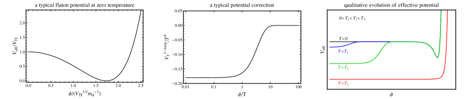
Figure 1: The zero-temperature potential of the flaton and its finite-temperature correction.

Thermal inflation begins when the energy density of other components decays to be as small as the potential energy of the flaton. If the Universe is dominated by radiation, the temperature at the beginning of thermal inflation, $T_{\rm begin}$, is given by $T_{\rm begin}=\left(\frac{30}{\pi^{2}g_{*}}V_{\rm TI}\right)^{1/4}$.

During thermal inflation, the potential energy of the false vacuum phase around the origin is larger than that of the true vacuum, meaning that we might expect tunneling from the false to the true vacuum. However, the tunneling rate is so small Yamamoto:1985rd that the flaton is assumed to be fixed at the origin until the dip almost disappears. Since the order of the curvature of the dip is determined by the temperature as $V_{\rm eff}^{\prime\prime}\sim{\cal O}(T^{2})$, thermal inflation ends when the temperature becomes as small as $m_{\phi}\approx m_{s}$. Therefore, by choosing $V_{\rm TI}$ and $m_{\phi}$, one can tune the duration of thermal inflation. Namely, the number of $e$-folds of thermal inflation is roughly given by

$${\cal N}=\log\left(\frac{T_{\rm begin}}{T_{\rm end}}\right)\sim\log\left(\frac{V_{\rm TI}^{\frac{1}{4}}}{m_{\phi}}\right)\,.$$ (7)

If we set $m_{\phi}=10^{3}$GeV and $V_{\rm TI}^{\frac{1}{4}}=10^{7}$GeV, we obtain ${\cal N}\sim 9$.

Here we consider how thermal inflation solves the gravitino problem gravitinoproblem . The gravitino, which only has suppressed interactions and hence a long lifetime, decays after BBN and its decay products affect the abundances of light elements. As such, we can constrain the abundance of the gravitino in the early Universe using observations Kawasaki:2004qu . We use the variable $Y_{3/2}=n_{3/2}/s$ to represent the comoving number density of gravitinos, since the entropy density, $s$, is proportional to $a^{-3}$ if there is no entropy production. Before the gravitinos decay, $Y_{3/2}$ is approximately proportional to the reheating temperature $T_{\rm R}$. Hence, if the reheating temperature is high, we have to decrease $Y_{3/2}$. According to Ref.Kawasaki:2004qu , $T_{\rm R}~{}\mbox{\raisebox{-4.30554pt}{$\stackrel{{\scriptstyle\textstyle>}}{{\textstyle\sim}}$ }}10^{6}\,{\rm GeV}$ may be problematic. A solution proposed in Ref.Lyth:1995hj is to increase the entropy density via flaton decay after thermal inflation. The ratio of the entropy densities before and after the flaton decay is

$$\frac{s_{\rm after}}{s_{\rm before}}\approx\frac{\frac{4}{3}\frac{V_{\rm TI}}{T_{\rm R,TI}}}{\frac{2\pi^{2}}{45}g_{*}(T_{\rm end})T_{\rm end}^{3}}=1.5\times 10^{17}\left(\frac{V_{\rm TI}^{\frac{1}{4}}}{10^{7}\,{\rm GeV}}\right)^{4}\left(\frac{T_{\rm R,TI}}{1\,{\rm GeV}}\right)^{-1}\left(\frac{T_{\rm end}}{1\,{\rm TeV}}\right)^{-3}\left(\frac{g_{*}(T_{\rm end})}{200}\right)^{-1}\,,$$ (8)

where $T_{\rm R,TI}$ is the reheating temperature associated with the flaton decay. Due to this significant entropy production the abundance of gravitinos is made harmless.

As another possibility, let us consider the case where the Universe transitions to thermal inflation after being dominated by oscillating moduli. Hereafter we use $\Phi$ to represent one of the moduli fields. Since the moduli start oscillating when the Hubble parameter becomes as small as the mass of the moduli ($m_{\Phi}$), they start oscillating before reheating if the reheating temperature is lower than $\sim\sqrt{m_{\Phi}M_{\rm Pl}}$. The energy density of the moduli at reheating is estimated as

$$\rho_{\Phi}({\rm at\,\,reheating})=\frac{1}{2}m_{\Phi}^{2}\Phi_{0}^{2}\times\left(\frac{a_{\rm osc}}{a_{\rm R}}\right)^{3}=\frac{1}{2}m_{\Phi}^{2}\Phi_{0}^{2}\times\left(\frac{H_{\rm R}}{H_{\rm osc}}\right)^{2}=\frac{1}{2}\Phi_{0}^{2}H_{\rm R}^{2}\,,$$ (9)

where $\Phi_{0}$ is the initial amplitude of the oscillating moduli and the subscript “osc” represents the value at the onset of oscillation. After reheating, since the temperature scales as $T\propto a^{-1}$, $\rho_{\Phi}$ scales as $\propto T^{3}$. Therefore $T_{\rm begin}$ is determined by

$$\frac{1}{2}\Phi_{0}^{2}H_{\rm R}^{2}\times\left(\frac{T_{\rm begin}}{T_{\rm R}}\right)^{3}=V_{\rm TI}\,,$$ (10)

then we obtain

$$T_{\rm begin}\approx 9.7\times 10^{5}\left(\frac{g_{*}}{200}\right)^{-1/3}\left(\frac{T_{\rm R}}{10^{9}\,{\rm GeV}}\right)^{1/3}\left(\frac{V_{\rm TI}^{\frac{1}{4}}}{10^{7}\,{\rm GeV}}\right)^{4/3}\left(\frac{\Phi_{0}}{M_{\rm Pl}}\right)^{1/3}\,{\rm GeV}\,.$$ (11)

On the other hand, if the reheating temperature is high, the oscillations begin in the radiation-dominated Universe, when

$$m_{\Phi}^{2}=H_{\rm osc}^{2}=\frac{\pi^{2}}{90}g_{*}\frac{T_{\rm osc}^{4}}{M_{\rm Pl}^{2}}\,,$$ (12)

is satisfied. If $\Phi_{0}$ is as large as $M_{\rm Pl}$, the energy density associated with the coherent oscillation of moduli soon becomes dominant. In this case $T_{\rm begin}$ is determined by

$$\frac{1}{2}m_{\Phi}^{2}\Phi_{0}^{2}\times\left(\frac{T_{\rm begin}}{T_{\rm osc}}\right)^{3}=V_{\rm TI}\,,$$ (13)

combining the above expressions we obtain

$$T_{\rm begin}\approx 3.4\times 10^{5}\left(\frac{g_{*}}{200}\right)^{-1/4}\left(\frac{V_{\rm TI}^{\frac{1}{4}}}{10^{7}\,{\rm GeV}}\right)^{4/3}\left(\frac{m_{\Phi}}{1\,{\rm TeV}}\right)^{-1/6}\left(\frac{\Phi_{0}}{M_{\rm Pl}}\right)^{2/3}\,{\rm GeV}\,.$$ (14)

Let us move on to the cosmological moduli problem. The moduli abundance $Y_{\Phi}=n_{\Phi}/s$ should also be small enough so as not to spoil BBN Ellis:1990nb . Assuming the moduli start oscillating before reheating, during the era when the energy density associated with the coherent oscillations of the inflaton dominate the Universe, the moduli abundance before flaton decay is evaluated as

$$Y_{\Phi}=\frac{\frac{1}{m_{\Phi}}\frac{1}{2}\Phi_{0}^{2}H_{\rm R}^{2}}{\frac{4}{3T_{\rm R}}\times 3M_{\rm Pl}^{2}H_{\rm R}^{2}}=\frac{1}{8}\frac{T_{\rm R}}{m_{\Phi}}\left(\frac{\Phi_{0}}{M_{\rm Pl}}\right)^{2}\,,$$ (15)

where we use eq. (9) and assume that there is no entropy production after reheating. After the flaton decays, by using eq. (8), $Y_{\Phi}$ becomes

$$Y_{\Phi,\,{\rm after}}\approx \,\,\frac{\pi^{2}}{240}g_{*}(T_{\rm end})\left(\frac{\Phi_{0}}{M_{\rm Pl}}\right)^{2}\frac{T_{\rm R}T_{\rm R,TI}T_{\rm end}^{3}}{m_{\Phi}V_{\rm TI}}\,$$

$$= \,\,8.2\times 10^{-13}\left(\frac{V_{\rm TI}^{\frac{1}{4}}}{10^{7}\,{\rm GeV}}\right)^{-4}\left(\frac{T_{\rm R}}{10^{9}\,{\rm GeV}}\right)\left(\frac{T_{\rm R,TI}}{1\,{\rm GeV}}\right)\left(\frac{T_{\rm end}}{m_{\Phi}}\right)^{3}\left(\frac{m_{\Phi}}{1\,{\rm TeV}}\right)\left(\frac{\Phi_{0}}{M_{\rm Pl}}\right)^{2}\left(\frac{g_{*}(T_{\rm end})}{200}\right)\,.$$ (16)

Therefore, with appropriate parameters, thermal inflation can make $Y_{\rm\Phi}$ small enough for successful BBN.

III flaton dynamics in a thermal bath

In this section, we consider the flaton dynamics based on finite-temperature field theory. In order to describe the dynamics of the expectation values of quantum fields in a thermal bath, we use the effective action method, which has been studied in several contexts FTEA ; Yamaguchi:1996dp ; Yokoyama:2004pf ; Greiner:1996dx based on the in-in or the closed time-path formalisms. Using this method, we can evaluate the evolution of expectation values by performing path integrals along two time paths, with two field variables $\phi_{\pm}$ defined on each path. Generally the effective action can be expressed as FTEA ; Yamaguchi:1996dp ; Yokoyama:2004pf ; Greiner:1996dx

$$\Gamma=S_{0}+\Gamma_{\rm R}+\Gamma_{\rm I}\,,$$ (17)

where $S_{0}$ is the tree level action, and $\Gamma_{\rm R}$ and $\Gamma_{\rm I}$, respectively, represent the real and imaginary parts coming from interactions. The imaginary part has the following structure

$$\exp\left[i\Gamma_{\rm I}\right] =\exp\left[-\frac{1}{2}\int d^{4}x_{1}d^{4}x_{2}A_{\rm a}(x_{1}-x_{2})\phi_{\Delta}(x_{1})\phi_{\Delta}(x_{2})+A_{\rm m}(x_{1}-x_{2})\phi_{\Delta}(x_{1})\phi_{\Delta}(x_{2})\phi_{c}(x_{1})\phi_{c}(x_{2})\right]\,,$$ (18)

and we can rewrite it as

$$\exp\left[i\Gamma_{\rm I}\right]=\int{\cal D}\xi_{\rm a}{\cal D}\xi_{\rm m}\,P[\xi_{\rm a}]P[\xi_{\rm m}]\exp\left[iS_{\rm noise}\right]\,,$$ (19)

where

$$P[\xi_{\rm a}] \propto\exp\left[-\frac{1}{2}\int d^{4}x_{1}d^{4}x_{2}\,\xi_{\rm a}(x_{1})A_{\rm a}^{-1}(x_{1}-x_{2})\xi_{\rm a}(x_{2})\right]\,,$$

$$P[\xi_{\rm m}] \propto\exp\left[-\frac{1}{2}\int d^{4}x_{1}d^{4}x_{2}\,\xi_{\rm m}(x_{1})A_{\rm m}^{-1}(x_{1}-x_{2})\xi_{\rm m}(x_{2})\right]\,,$$

$$S_{\rm noise} =\int d^{4}x\,\left[\xi_{\rm a}(x)\phi_{\Delta}(x)+\xi_{\rm m}(x)\phi_{\Delta}(x)\phi_{c}(x)\right]\,,$$

$$\phi_{c}=\frac{\phi_{+}+\phi_{-}}{2}\,,\quad\phi_{\Delta}=\phi_{+}-\phi_{-}\,.$$ (20)

We can interpret the new variables $\xi_{\rm a}$ and $\xi_{\rm m}$ as stochastic noises whose probability distributions are given by $P[\xi_{\rm a}]$ and $P[\xi_{\rm m}]$, respectively. Finally the equation of motion for $\phi_{c}$, which is obtained by varying the effective action with respect to $\phi_{\Delta}$, becomes the Langevin equation

$$\Box\phi(x)+V_{\rm eff}^{\prime}[\phi]+\int_{-\infty}^{t}dt^{\prime}\int d^{3}x^{\prime}\,B_{\rm a}(x-x^{\prime})\phi(x^{\prime})+\phi(x)\int_{-\infty}^{t}dt^{\prime}\int d^{3}x^{\prime}\,B_{\rm m}(x-x^{\prime})\phi^{2}(x^{\prime})$$

$$= \xi_{\rm a}(x)+\xi_{\rm m}(x)\phi(x)\,.$$ (21)

We briefly see specific examples studied in Ref. Yokoyama:2004pf . An interaction term ${\cal L}_{\rm int}=-\lambda^{2}\chi^{2}\phi^{2}$, where $\chi$ is a real scalar field, leads to both additive and multiplicative noises and the corresponding non-local terms. Functions $A$ and $B$ for additive noise and the correspondent non-local terms in Fourier space are calculated as

$$A_{\rm a}(\omega,\vec{k})=-16\pi i\lambda^{4}\int \frac{d^{3}q_{1}}{(2\pi)^{3}}\frac{d^{3}q_{2}}{(2\pi)^{3}}\frac{d^{3}q_{3}}{(2\pi)^{3}}(2\pi)^{3}\delta^{3}(\vec{q}_{1}+\vec{q}_{2}+\vec{q}_{3}-\vec{k})\frac{1}{8\omega_{q_{1}}\omega_{q_{2}}\omega_{k-q_{1}-q_{2}}}$$

$$\times\Large[ \left\{(1+n_{q_{1}})(1+n_{q_{2}})(1+n_{q_{3}})+n_{q_{1}}n_{q_{2}}n_{q_{3}}\right\}\delta(\omega-\omega_{q_{1}}-\omega_{q_{2}}-\omega_{q_{3}})$$

$$+ \left\{(1+n_{q_{1}})(1+n_{q_{2}})n_{q_{3}}+n_{q_{1}}n_{q_{2}}(1+n_{q_{3}})\right\}\delta(\omega-\omega_{q_{1}}-\omega_{q_{2}}+\omega_{q_{3}})$$

$$+ \left\{(1+n_{q_{1}})n_{q_{2}}(1+n_{q_{3}})+n_{q_{1}}(1+n_{q_{2}})n_{q_{3}}\right\}\delta(\omega-\omega_{q_{1}}+\omega_{q_{2}}-\omega_{q_{3}})$$

$$+ \left\{n_{q_{1}}(1+n_{q_{2}})(1+n_{q_{3}})+(1+n_{q_{1}})n_{q_{2}}n_{q_{3}}\right\}\delta(\omega+\omega_{q_{1}}-\omega_{q_{2}}-\omega_{q_{3}})$$

$$+ \left\{(1+n_{q_{1}})n_{q_{2}}n_{q_{3}}+n_{q_{1}}(1+n_{q_{2}})(1+n_{q_{3}})\right\}\delta(\omega-\omega_{q_{1}}+\omega_{q_{2}}+\omega_{q_{3}})$$

$$+ \left\{n_{q_{1}}(1+n_{q_{2}})n_{q_{3}}+(1+n_{q_{1}})n_{q_{2}}(1+n_{q_{3}})\right\}\delta(\omega+\omega_{q_{1}}-\omega_{q_{2}}+\omega_{q_{3}})$$

$$+ \left\{n_{q_{1}}n_{q_{2}}(1+n_{q_{3}})+(1+n_{q_{1}})(1+n_{q_{2}})n_{q_{3}}\right\}\delta(\omega+\omega_{q_{1}}-\omega_{q_{2}}+\omega_{q_{3}})$$

$$+ \left\{n_{q_{1}}n_{q_{2}}n_{q_{3}}+(1+n_{q_{1}})(1+n_{q_{2}})(1+n_{q_{3}})\right\}\delta(\omega+\omega_{q_{1}}+\omega_{q_{2}}+\omega_{q_{3}})\Large]\,,$$ (22)

$$B_{\rm a}(\omega,\vec{k})=8\pi\lambda^{4}\int \frac{d^{3}q_{1}}{(2\pi)^{3}}\frac{d^{3}q_{2}}{(2\pi)^{3}}\frac{d^{3}q_{3}}{(2\pi)^{3}}(2\pi)^{3}\delta^{3}(\vec{q}_{1}+\vec{q}_{2}+\vec{q}_{3}-\vec{k})\frac{1}{8\omega_{q_{1}}\omega_{q_{2}}\omega_{q_{3}}}$$

$$\times\Large[ \left\{(1+n_{q_{1}})(1+n_{q_{2}})(1+n_{q_{3}})-n_{q_{1}}n_{q_{2}}n_{q_{3}}\right\}\delta(\omega-\omega_{q_{1}}-\omega_{q_{2}}-\omega_{q_{3}})$$

$$+ \left\{(1+n_{q_{1}})(1+n_{q_{2}})n_{q_{3}}-n_{q_{1}}n_{q_{2}}(1+n_{q_{3}})\right\}\delta(\omega-\omega_{q_{1}}-\omega_{q_{2}}+\omega_{q_{3}})$$

$$+ \left\{(1+n_{q_{1}})n_{q_{2}}(1+n_{q_{3}})-n_{q_{1}}(1+n_{q_{2}})n_{q_{3}}\right\}\delta(\omega-\omega_{q_{1}}+\omega_{q_{2}}-\omega_{q_{3}})$$

$$+ \left\{n_{q_{1}}(1+n_{q_{2}})(1+n_{q_{3}})-(1+n_{q_{1}})n_{q_{2}}n_{q_{3}}\right\}\delta(\omega+\omega_{q_{1}}-\omega_{q_{2}}-\omega_{q_{3}})$$

$$+ \left\{(1+n_{q_{1}})n_{q_{2}}n_{q_{3}}-n_{q_{1}}(1+n_{q_{2}})(1+n_{q_{3}})\right\}\delta(\omega-\omega_{q_{1}}+\omega_{q_{2}}+\omega_{q_{3}})$$

$$+ \left\{n_{q_{1}}(1+n_{q_{2}})n_{q_{3}}-(1+n_{q_{1}})n_{q_{2}}(1+n_{q_{3}})\right\}\delta(\omega+\omega_{q_{1}}-\omega_{q_{2}}+\omega_{q_{3}})$$

$$+ \left\{n_{q_{1}}n_{q_{2}}(1+n_{q_{3}})-(1+n_{q_{1}})(1+n_{q_{2}})n_{q_{3}}\right\}\delta(\omega+\omega_{q_{1}}-\omega_{q_{2}}+\omega_{q_{3}})$$

$$+ \left\{n_{q_{1}}n_{q_{2}}n_{q_{3}}-(1+n_{q_{1}})(1+n_{q_{2}})(1+n_{q_{3}})\right\}\delta(\omega+\omega_{q_{1}}+\omega_{q_{2}}+\omega_{q_{3}})\Large]\,,$$ (23)

where $\omega_{q_{i}}=\sqrt{|\vec{q}_{i}|^{2}+m_{\chi}^{2}}$ and $n_{q_{i}}=\frac{1}{e^{\beta\omega_{q_{i}}}-1}$. For the multiplicative noise and corresponding non-local term, we find

$$A_{\rm m}(\omega,\vec{k})=2\pi\lambda^{4}\int\frac{d^{3}q}{(2\pi)^{3}}\frac{1}{\omega_{q}\omega_{k-q}}\times\Large[ \left\{(1+n_{q})(1+n_{k-q})+n_{q}n_{k-q}\right\}\delta(\omega-\omega_{q}-\omega_{k-q})$$

$$+ \left\{(1+n_{q})n_{k-q}+n_{q}(1+n_{k-q})\right\}\delta(\omega-\omega_{q}+\omega_{k-q})$$

$$+ \left\{(n_{q}(1+n_{k-q})+(1+n_{q})n_{k-q}\right\}\delta(\omega+\omega_{q}-\omega_{k-q})$$

$$+ \left\{n_{q}n_{k-q}+(1+n_{q})(1+n_{k-q})\right\}\delta(\omega+\omega_{q}+\omega_{k-q})\Large]\,,$$ (24)

$$B_{\rm m}(\omega,\vec{k})=-2\pi i\lambda^{4}\int\frac{d^{3}q}{(2\pi)^{3}}\frac{1}{\omega_{q}\omega_{k-q}}\times\Large[ \left\{(1+n_{q})(1+n_{k-q})-n_{q}n_{k-q}\right\}\delta(\omega-\omega_{q}-\omega_{k-q})$$

$$+ \left\{(1+n_{q})n_{k-q}-n_{q}(1+n_{k-q})\right\}\delta(\omega-\omega_{q}+\omega_{k-q})$$

$$+ \left\{(n_{q}(1+n_{k-q})-(1+n_{q})n_{k-q}\right\}\delta(\omega+\omega_{q}-\omega_{k-q})$$

$$+ \left\{n_{q}n_{k-q}-(1+n_{q})(1+n_{k-q})\right\}\delta(\omega+\omega_{q}+\omega_{k-q})\Large]\,.$$ (25)

Though the noise terms generally consist of both additive noise, $\xi_{\rm a}$, and multiplicative noise, $\xi_{\rm m}\phi$, we focus on the additive noise term since the former is more important to trigger phase transition. This noise term is related to the “friction” term through the fluctuation-dissipation relation Yokoyama:2004pf ; Greiner:1996dx

$$\frac{\rm noise\,\,correlation}{\rm dissipation\,\,coefficient}=\frac{A_{\rm a}(\omega,\vec{k})}{iB_{\rm a}(\omega,\vec{k})/2\omega}=\omega\frac{e^{\omega/T}+1}{e^{\omega/T}-1}\to 2T\,\,(T\gg\omega)\,.$$ (26)

In Ref. Yamaguchi:1996dp it was shown that the damping scale of the fermionic noise correlation is independent of the mass of the fermion, which is different from the bosonic noise whose correlation damps exponentially above the mass scale. Therefore, in the high-temperature regime $T\gg m$, the dominant noise component comes from interactions with fermions. More quantitatively, the correlation function for fermionic noise can be expressed as

$$\langle\xi(t,\vec{x})\xi(t,\vec{x}^{\prime})\rangle\propto\frac{T^{4}}{r^{2}}e^{-2\pi rT}\,,\quad{\rm for}\,\,\,r\gg\frac{1}{\pi T}\,,\quad(r=|\vec{x}-\vec{x}^{\prime}|)\,.$$ (27)

From this expression we take the correlation length of thermal noise as $(\pi T)^{-1}$. This length scale is very important in estimating the typical value of the flaton at finite temperature. Here let us take a quick look at this typical field value, as this will help us to understand the results of numerical simulations later. The form of the effective potential is too complicated to be well approximated by a simple polynomial function, so for simplicity let us neglect the potential here. Following Ref. Yamaguchi:1997sy , the mean square value of the coarse-grained field $\phi$ over the spatial scale $R$ is given by

$$\langle\phi^{2}\rangle_{\rm R}=\frac{1}{2\pi^{2}}\int_{0}^{\infty}dk\,k\left(\frac{1}{2}+\frac{1}{e^{\frac{k}{T}}-1}\right)\,W(k,R)^{2}\,,$$ (28)

where $W(k,R)$ is the coarse-graining window function. As an example, if we take the Gaussian function

$$W(k,R)=e^{-\frac{1}{2}k^{2}R^{2}}\,,$$ (29)

we obtain $\sqrt{\langle\phi^{2}\rangle}\approx 0.43T$ for $R=(\pi T)^{-1}$.

Since the correlation length of the noise is $\sim(\pi T)^{-1}$, we can treat the noise as being uncorrelated on larger scales. The same is true for the temporal noise correlation, since it is suppressed exponentially for $\Delta t>(\pi T)^{-1}$. As such, the noise term can be approximated by a white, Gaussian random variable when we consider dynamics on spatial and temporal scales that are larger than the above correlation length. Hence we use the following simple EoM.

$$\ddot{\phi}(\vec{x},t)-\vec{\nabla}^{2}\phi(\vec{x},t)+\eta\dot{\phi}(\vec{x},t)+V_{\rm eff}^{\prime}[\phi]=\xi(\vec{x},t)\,,$$ (30)

where the correlation function of the noise term is

$$\left\langle\xi(\vec{x},t)\xi(\vec{x}^{\prime},t^{\prime})\right\rangle=D\delta(t-t^{\prime})\delta^{3}(\vec{x}-\vec{x}^{\prime})\,.$$ (31)

The fluctuation-dissipation relation in this simple EoM is

$$\frac{D}{\eta}=2T\,.$$ (32)

Due to the fluctuation-dissipation relation, equilibrium values do not depend on the friction coefficient $\eta$. Its value is related with the decay rate of $\phi$ particle if $\phi$ is oscillating FTEA ; Yokoyama:2004pf ; Greiner:1996dx . On dimensional grounds we can take $\Gamma\propto T$. Since the value of $\eta$ only determines the time scale on which the system approaches equilibrium, here we simply take $\eta=T$ as strong enough couplings between the flaton and the thermal bath are required for successful thermal inflation. Then the ratio of the equilibration timescale to the cosmic expansion timescale is

$$\frac{\rm equilibration\,\,timescale}{\rm Hubble\,\,time}\sim\frac{\eta^{-1}}{H^{-1}}=\frac{T^{-1}}{H^{-1}}\sim\begin{cases}\frac{T}{M_{\rm Pl}}&(\rm RD\,\,era)\,,\\ &\\ \frac{V_{\rm TI}^{\frac{1}{2}}}{M_{\rm Pl}\,T}&(\rm during\,\,thermal\,\,inflation)\,.\end{cases}$$ (33)

We see that this ratio is much smaller than unity in both the RD era and the period of thermal inflation, from which we can conclude that the equilibration time is still much shorter than the Hubble time even if we take other choices for the value of $\eta$. This huge difference between the two timescales allows us to safely ignore the Hubble expansion in simulations we show later.

IV Setup of Numerical Simulations

In this section we summarize the details of our three-dimensional lattice simulation. We solved the equation of motion given by eq. (30) by the second-order explicit Runge-Kutta method with the second-order finite differences approximating the spatial derivatives. The basic setup is the same as in Ref.Yamaguchi:1996dp . In numerical calculations we use dimensionless variables like $\tilde{x}=Tx$, $\tilde{t}=Tt$, $\tilde{\phi}=\phi/T$, and $\tilde{\xi}=\xi/T^{3}$ since the scale of interest is deeply related to the temperature.

The noise correlation function on the lattice becomes

$$\langle\xi(\vec{x}_{i},t_{m})\xi(\vec{x}_{j},t_{n})\rangle=2\eta\delta(t_{m}-t_{n})\delta^{3}(\vec{x}_{i}-\vec{x}_{j})\to\frac{2\eta}{\Delta t(\Delta x)^{3}}\delta_{m,n}\delta_{i,j}\,,$$ (34)

since on the lattice the delta functions are properly replaced as $\delta(t_{m}-t_{n})\to(\Delta t)^{-1}\delta_{m,n}$ and $\delta^{3}(\vec{x}_{i}-\vec{x}_{j})\to(\Delta x)^{-3}\delta_{i,j}$. The value of noise variable on each lattice is given by

$$\xi(\vec{x}_{i},t_{m})=\left(\frac{2\eta}{\Delta t(\Delta x)^{3}}\right)^{\frac{1}{2}}{\mathcal{G}}_{i,m}\,,$$ (35)

where ${\mathcal{G}}$ is a standard Gaussian random variable.

We also define approximation function of the potential term, which is shown in Appendix. As can be seen later, the quantitative shape of the effective potential is very sensitive to the temperature, especially at the end of thermal inflation. Therefore we use the above approximation function both in the lattice simulation and semi-analytic calculation.

We choose the initial condition for simulations as

$$\phi(\vec{x},t=0)=\dot{\phi}(\vec{x},t=0)=0\,.$$ (36)

Although this is an admittedly unrealistic initial condition, we have confirmed that the field quickly reaches the thermal configuration compared to the typical duration of simulation time and the timescale of the temperature variation.

With the above settings we use the $256^{3}$ lattice points and $m_{\phi}$ (and $m_{\rm b}$ in eq. (6))$=10^{3}$ and $10^{2}$ GeV, but the qualitative results do not depend on these mass values.

V Results of Numerical Simulations

V.1 phase 1: before thermal inflation

A necessary initial condition for the flaton to drive thermal inflation is that the field value of the flaton should be homogeneously close to zero before thermal inflation begins. However, the form of the 1-loop effective potential suggests that there is more than one local minimum, and if the flaton field is trapped in the true vacuum in some spatial regions, the thermal inflation scenario does not work. In order to determine whether or not this problem is encountered, we simulated the time evolution of the flaton from a very high temperature, $T_{\rm 0}$, to the temperature at which thermal inflation begins.

The “high” temperature $T_{\rm 0}$ is determined by the following consideration. In order to realize a situation where the typical value of the flaton is $\phi_{\rm vev}$ ($\equiv\sqrt{3V_{\rm TI}}/m_{\phi}$, the vacuum expectation value at $T=0$), we first perform a simulation at $T=\phi_{\rm vev}$, expecting $\sqrt{\langle\phi^{2}\rangle}\approx T\approx\phi_{\rm vev}$. At this temperature the shape of the effective potential becomes like the potential labelled “$T=T_{1}$” in the right panel of Fig.1. We then perform a second simulation, setting the temperature to half of that in the previous simulation and using the final configuration of the previous simulation to determine the initial conditions. Since we fix the gridsize of the simulation and the value of the lattice spacing normalized by the temperature, the physical size of the second simulation box is larger than that of the previous, hotter simulation. We therefore use periodic boundary conditions and define the initial condition for $\phi$ and $\dot{\phi}$ as averaged quantities of the previous values of close grids on each new grids. Repeating this procedures $N$ times we can follow the flaton dynamics from $T=T_{0}$ to $T=T_{0}\times 2^{-N}\sim T_{\rm begin}$.

In the numerical simulations we consider corrections to the potential coming from a single bosonic and single fermionic degree of freedom. In order to try and establish the importance of the thermal effects we perform simulations with two choices of the coupling constants appearing in eq. (6). Hereafter we refer to these two choices as the strongly and weakly coupled cases, and they correspond to taking $\lambda_{\rm b}=g_{\rm b}=\lambda_{\rm f}=g_{\rm f}=1$ and $\lambda_{\rm b}=g_{\rm b}=\lambda_{\rm f}=g_{\rm f}=0.1$ respectively. We also consider two different scenarios. In the first scenario thermal inflation is preceded by moduli domination (MD$\to$TI) and in the second scenario thermal inflation is preceded by radiation domination (RD$\to$TI). The results of one example simulation are shown in Fig.2. For the form of effective potential used in this study, we confirm that the typical value of the flaton is $\sqrt{\langle\phi^{2}\rangle}\approx T$, regardless of the temperature before thermal inflation. In other words, we do not see any spatial regions where the field value remains so large that the flaton potential energy becomes inhomogeneous and ruins the thermal inflation scenario.

We close this subsection with comments on the validity of our multistage simulation. The result shown in Fig. 2 confirms us that we properly follow the dynamics of the flaton from a high temperature to $T_{\rm begin}$, with multistage simulation. Since the equilibration timescale ($\sim\eta^{-1}$) is much shorter than that of temperature change ($\sim H^{-1}$), the system approaches the equilibrium rapidly enough in each simulation with a fixed temperature. In other words, even though we impose out-of-equilibrium initial condition which is simply connected by the previous simulation where the temperature is set twice as hot, we can realize the equilibrium distribution ($\sqrt{\langle\phi^{2}\rangle}\sim T$) by performing a simulation for a longer time than $\eta^{-1}$ (but much shorter than $H^{-1}$). Therefore repetitive simulations enable us to consider a system in quasi-equilibrium state for a longer time than Hubble time without including the exact change in temperature. The smooth change of the root mean square (RMS) value obtained in Fig. 2 justifies a factor of 2 change of the temperature at each step is small enough to warrant the adiabatic change of the temperature in the sequential simulations. As for the maximum value, we note that for random $256^{3}$ realization of Gaussian distribution, the probability the maximun exceeds 6.2$\sigma$ (5.6T) is 1 $\%$ and that it lies lower than 5.2 $\sigma$ (4.6T) is also 1$\%$. Although the field value at each point is correlated with nearby points, we find one-point distribution function is close to a Gaussian distribution. Hence we may conclude the observed maximum values in Fig. 2 are also in accordance with the entire distribution.

scenario	couplings	$T_{\rm begin}$[GeV]	$\phi_{\rm vev}(=T_{0})$[GeV]
MD $\to$ TI	strong	$2.1\times 10^{6}$	$3.7\times 10^{12}$
MD $\to$ TI	weak	$1.7\times 10^{7}$	$8.3\times 10^{13}$
RD $\to$ TI	strong	$2.1\times 10^{6}$	$6.0\times 10^{10}$
RD $\to$ TI	weak	$1.7\times 10^{7}$	$3.9\times 10^{12}$

Table 1: The temperature at the beginning of thermal inflation and VEV of the flaton. Since the ratio of these values is ${\cal O}(10^{6})\sim 2^{20}$, we performed about 20 simulations to follow the flaton dynamics from $T_{0}$ to $T_{\rm begin}$.

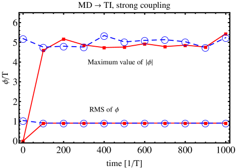
Figure 2: The results of one example multistage lattice simulation that was performed assuming moduli-domination before thermal inflation and strong coupling to the fields in the thermal bath. In other cases the results are qualitatively the same. The root mean square of $\phi$ and the maximum value of $|\phi|$ in the first and the last simulation at each reference time are shown. The red lines with square vertices are the results of the first (hot) simulation and the dashed blue lines with circular vertices are those of the last simulation, where $T\sim T_{\rm begin}$. Since we impose the initial conditions $\phi=\dot{\phi}=0$ in the first simulation and the initial conditions for the following simulations are determined sequentially by the final configuration of the preceding, higher temperature simulation, the flaton distribution at each first reference time is not the equilibrium configuration.

V.2 phase 2: at the end of thermal inflation

It is believed that thermal inflation ends with a first-order phase transition accompanied by the formation of bubbles, and that the collision of these bubbles then leads to gravitational wave production. Here we briefly review the theory of tunneling at a finite temperature and define the percolation temperature at which the bubbles collide and start generating gravitational waves.

The tunneling rate per unit volume at temperature $T$ is estimated as Linde:1980tt

$$\Gamma(T)\sim T^{4}e^{-\frac{S_{3}}{T}}\,,$$ (37)

where $S_{3}$ is the Euclidean action after performing the time integral,

$$S_{3}=\int d^{3}x\left(\frac{1}{2}\left(\nabla\phi\right)^{2}+V(\phi)\right)\,.$$ (38)

The dominant contribution to the tunneling rate comes from the solution of the equation of motion,

$$\frac{d^{2}\phi}{dr^{2}}+\frac{2}{r}\frac{d\phi}{dr}-\frac{dV}{d\phi}=0\,,\quad(r=|\vec{x}|)$$ (39)

under the boundary conditions $\phi(r=\infty)=0$ and $\left.\frac{d\phi}{dr}\right|_{r=0}=0$.

The fraction of spatial regions occupied by bubbles can be written as Guth:1981uk

$$F(t)=1-e^{-P(t)}\,,$$ (40)

where the function $P(t)$ is given by

$$P(t)= \int^{t}dt^{\prime}\,\Gamma(t^{\prime})\frac{4\pi}{3}\left(\int_{t^{\prime}}^{t}dt^{\prime\prime}\,\frac{a(t)}{a(t^{\prime\prime})}\right)^{3}$$

$$= \frac{4\pi}{3}\int^{t}dt^{\prime}\,\Gamma(t^{\prime})\frac{1}{H^{3}}\left(e^{H(t-t^{\prime})}-1\right)^{3}\,.$$ (41)

Making use of eq.(37) we can rewrite this in terms of temperature as

$$P(T)=\frac{4\pi}{3}\int_{T}^{\infty}dT^{\prime}\,\frac{T^{\prime 3}}{H^{4}}\left(\frac{T^{\prime}}{T}-1\right)^{3}e^{-\frac{S_{3}(T)}{T}}\,.$$ (42)

In this paper we define the percolation temperature as $F(T=T_{\rm p})=0.5$ . Note that since the exponential factor $\exp[-S_{3}(T)/T]$ is very sensitive to the temperature and quickly becomes small when we take a large value of $T$, it is sufficient to take the upper limit of the integral to be some finite value. For example, it is enough to take it as $2T_{\rm curv}$, where $T_{\rm curv}$ is the temperature at which the curvature of the potential becomes zero. After evaluating the above quantities numerically, we find that the difference between the percolation temperature $T_{\rm p}$ and $T_{\rm curv}$ is tiny, so that the Universe becomes filled with critical bubbles almost immediately after bubble formation effectively begins.

From the above consideration based on the shape of the flaton effective potential, we may expect that thermal inflation ends with a first-order phase transition characterized by critical bubble formation. However, this description is based on the assumption that the flaton is well within the false vacuum phase before bubble nucleation occurs.

We see from Fig.3 that around the percolation temperature the potential barrier is located at $\phi\ll T$ and the height of the barrier is much smaller than $T^{4}$. Taking thermal fluctuations into account, since the width of the field distribution is $\sqrt{\langle\phi^{2}\rangle}\approx T$, we conclude that the small potential barrier cannot trap the flaton in the false vacuum phase until the temperature becomes as small as the temperature at which critical bubble nucleation occurs. This means that the two phases coexist well before the percolation epoch in the bubble nucleation picture, and the phase transition proceeds with phase-mixing. As such, the standard description of the end of thermal inflation in terms of a strong first-order phase transition which is accompanied with bubble formation is inappropriate.

Now let us investigate more quantitatively the failure of critical bubble formation as a description of the end of thermal inflation. The width of the wall trapping the flaton is broad at high temperatures and gradually becomes thin as the temperature drops. We define the width in field space, $\phi_{\rm wid}$, at temperature $T$, as

$$V_{\rm eff}[\phi=\phi_{\rm wid},T]=V_{\rm eff}[\phi=0,T]\,.$$ (43)

Since the shape of the effective potential depends on temperature, we obtain $\phi_{\rm wid}(T)$ by solving the above equation. As a typical temperature at which phase-mixing occurs, we define the temperature $T_{\rm sub}$ as

$$\phi_{\rm wid}(T=T_{\rm sub})=T_{\rm sub}\,,$$ (44)

i.e. $T_{\rm sub}$ is the temperature at which the width of the potential wall becomes as small as the temperature. As we see from the simulations in the previous subsections and the analytical estimation (eq. (28)), the typical value of $\phi$ is as large as $T$. Therefore, at $T=T_{\rm sub}$, and if the height of the potential barrier is small enough, spatial regions in which the flaton lies outside of the potential dip are ubiquitous in the Universe. We call such regions subcritical bubbles subcriticalbubble , which are continuously created and destroyed by thermal fluctuations and hence differ from the critical bubbles which only grow after being nucleated by tunneling. For the effective potential we study in this paper, the relations $T_{\rm sub}>T_{\rm p}$ and $F(T_{\rm sub})\ll 1$ hold. Therefore, at $T=T_{\rm sub}$ the flaton is no longer trapped at the local minimum at the origin, meaning that there are practically no critical bubbles. Specific values are shown in Table 2. We would like to make a comment on the temperature at the end of thermal inflation, $T_{\rm end}$ quantitatively. In Section II we estimated $T_{\rm end}\sim m_{\phi}$. Table 2, however, shows that while $T_{\rm curv}$, $T_{\rm p}$, and $T_{\rm sub}$ coincide with each other within $5\%$ they deviate from $m_{\phi}$ by a factor of 5 - 40. Hence we should use $T_{\rm end}\sim T_{\rm sub}$ to estimate the proper duration of thermal inflation.

By performing numerical simulations at $T=T_{\rm sub}$ we are able to verify that the height of the potential barrier is small enough for the flaton to escape from $\phi=0$. In some cases we found that the flaton rolls down to the bottom of the potential – meaning that thermal inflation ends at $T>T_{\rm sub}$ – and in other cases we found that the flaton remained around the origin, but with a distribution width that was broader than the potential well. We thus see that all cases deviate from the standard scenario in which thermal inflation ends as the result of a strong first-order phase transition. We summarize the dependence of the potential shape on temperature in Fig.4 schematically.

scenario	couplings	$T_{\rm curv}$[GeV]	$T_{\rm p}$[GeV]	$T_{\rm sub}$[GeV]	$F(T_{\rm sub})$	simulated $\sqrt{\langle\phi^{2}\rangle}$ at $T_{\rm sub}$
MD $\to$ TI	strong	5230	5239 ($2\times 10^{-3}$)	5502($5\times 10^{-2}$)	$10^{-84}$	$\phi_{\rm vev}$
MD $\to$ TI	weak	41216.96	41216.97($4\times 10^{-7}$)	41378($4\times 10^{-3}$)	less than $10^{-2000}$	$0.91T$
RD $\to$ TI	strong	5230	5252 ($4\times 10^{-3}$)	5502($5\times 10^{-2}$)	$10^{-77}$	$\phi_{\rm vev}$
RD $\to$ TI	weak	41216.96	41216.97($4\times 10^{-7}$)	41378($4\times 10^{-3}$)	less than $10^{-2000}$	$0.91T$

Table 2: Specific temperature values for four different scenarios. In all four scenarios we take $m_{\phi}=1\,{\rm TeV}$. Since the temperatures themselves are almost the same, we also show the relative differences $(T_{\rm p}-T_{\rm curv})/T_{\rm curv}$ and $(T_{\rm sub}-T_{\rm curv})/T_{\rm curv}$ in brackets. In evaluating $T_{\rm p}$ and $F(T)$, we fix the value of $V_{\rm TI}$ so that thermal inflation begins at $T=T_{\rm curv}\times e^{6}$. The RMS values of $\phi$ at $T=T_{\rm sub}$, obtained by simulations with duration $t=2000/T$, are also shown. In the two strongly-coupled cases the flaton leaves the origin and settles in its VEV. In the two weakly-coupled cases the flaton stays at the origin, but the width of its distribution function is as broad as the barrier. Though the potential barrier is negligible, the potential force arising from the tachyonic mass term is also so weak that it may take a long time to displace the flaton from the origin.

Figure 3: Some examples of the effective potential at $T=T_{\rm curv}$, $T_{\rm p}$, and $T_{\rm sub}$ are shown. Since at $T=T_{\rm p}$ the local maximum is located at $\phi<T$ and its height is much smaller than $T^{4}$, the flaton is able to escape the local minimum and critical bubble formation theory is not applicable.

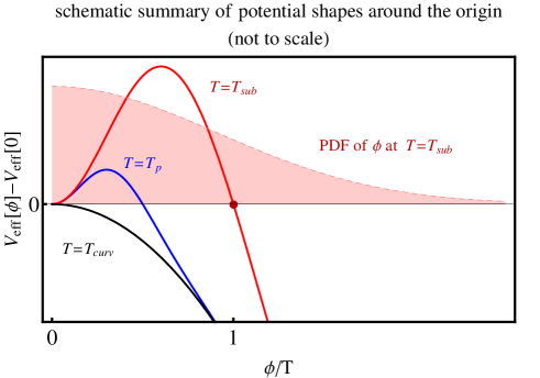
Figure 4: A schematic relation of the potential shapes at $T=T_{\rm sub}$, $T_{\rm p}$, and $T_{\rm curv}$. We also show the probability distribution function of the flaton at $T=T_{\rm sub}$, which indicates that subcritical bubbles are abundant in the Universe at $T=T_{\rm sub}$.

VI Conclusion

In this paper we studied the effect of thermal fluctuations on the thermal inflation scenario. Thermal inflation is a short period of accelerated expansion after reheating and provides a way to dilute dangerous moduli and gravitinos in order to make theories based on supersymmetry compatible with cosmological observations. Thermal inflation is driven by the flaton potential energy at the origin with the help of thermal corrections. Since the thermal environment gives rise to thermal fluctuations as well, we used lattice simulations to study the dynamics of the flaton taking into account the 1-loop effective potential, thermal fluctuations and the dissipation term. First we studied the effects of thermal fluctuations before thermal inflation. Though the effective potential contains multiple local minima during the course of the evolution of the Universe, the flaton settles at the origin before thermal inflation even when thermal fluctuations are taken into account. Therefore the scenario of thermal inflation may be feasible. Second, we find that thermal inflation ends with a cross over phase transition. The tunneling rate of the flaton from the origin of the potential is so small that the tunneling does not occur until the position of the potential barrier becomes very close to the origin. However, since the height of the barrier is much smaller than $T^{4}$, the flaton can escape over the barrier before tunneling occurs. Though the form of the effective potential suggests that thermal inflation ends with a first-order phase transition accompanied by bubble formation, thermal fluctuations make the transition to proceed through phase mixing, which is characterized by subcritical bubbles. As such, we cannot expect critical bubble formation and the production of gravitational waves.

Appendix : constructing approximation functions of the potential term

In this section, we consider the approximation of Eq. (3), which determines the functional shape of the thermal correction to the flaton potential. Expanding the integrand of Eq. (3), we can perform the integration term by term,

$$J_{\pm}(y) =\mp\frac{1}{2\pi^{2}}\sum_{n=1}^{\infty}\frac{(\pm 1)^{n}}{n}\int_{0}^{\infty}\!dx\,x^{2}e^{-n\sqrt{x^{2}+y^{2}}},$$

$$=\mp\frac{y^{2}}{2\pi^{2}}\sum_{n=1}^{\infty}\frac{(\pm 1)^{n}}{n^{2}}K_{2}(ny),$$ (45)

where $K_{2}(x)$ is the modified Bessel function of the second kind. The derivative of $J(y)$ with respect to $y$, which appears in the field equation, (30), is calculated as

$$\frac{dJ}{dy} =\pm\frac{y^{2}}{2\pi^{2}}\sum_{n=1}^{\infty}\frac{(\pm 1)^{n}}{n}K_{1}(ny).$$ (46)

For convenience, we define the shape function,

$$S_{\pm}(y)\equiv\sum_{n=1}^{\infty}\frac{(\pm 1)^{n}}{n}K_{1}(ny).$$ (47)

The modified Bessel function $K_{1}(z)$ for small $z$ can be approximated as

$$K_{1}(z)\approx\frac{1}{z}.$$ (48)

Therefore, the shape function for small $y$ becomes

$$S_{\pm}(y)\approx\frac{1}{y}\sum_{n=1}^{\infty}\frac{(\pm 1)^{n}}{n^{2}}=\frac{1}{y}\times\begin{cases}\displaystyle\zeta(2),&\mbox{for }+\\ \displaystyle-\frac{\zeta(2)}{2}.&\mbox{for }-\end{cases}$$ (49)

Away from $y=0$ this approximation breaks down almost immediately. Moreover, it is difficult to achieve better accuracy by simply retaining more terms in the expansion in Eq. (48), since there are logarithmic terms like $\ln z$, meaning that we cannot take the infinite summation analytically. Instead, we use the following ansatz,

$$\widetilde{S}^{(0)}_{+}(y) =\frac{e^{-y}}{y}\left(\zeta(2)+a_{1}y+a_{2}y^{2}+a_{3}y^{3}\right),$$ (50)

$$\widetilde{S}^{(0)}_{-}(y) =\frac{e^{-y}}{y}\left(-\frac{\zeta(2)}{2}+b_{1}y+b_{2}y^{2}+b_{3}y^{3}+b_{4}y^{4}\right),$$ (51)

where $a_{i}$ and $b_{i}$ are determined by requiring a good fit with the shape function in the limited region $0\leq y\leq 2$; we obtain $a_{i}=(0.146773,0.106023,-0.0248936)$ and $b_{i}=(-0.772073,0.163142,-0.0547415,0.0107667)$.

In the opposite limit, for large $y$ we can truncate the infinite summation in Eq. (47) at relatively small $n$ thanks to the asymptotically exponential decay of $K_{1}(ny)$. Here we take the summation up to $n=2$. We also use the asymptotic expansion of the modified Bessel functions. To guarantee accuracy, we expand $K_{1}(y)$ up to $y^{-3}$ and $K_{1}(2y)$ up to $y^{-1}$. Eventually we obtain

$$\widetilde{S}^{(\infty)}_{\pm}(y)=\pm\sqrt{\frac{\pi}{2y}}e^{-y}\left(1+\frac{3}{8y}-\frac{15}{128y^{2}}+\frac{105}{1024y^{3}}\right)+\sqrt{\frac{\pi}{16y}}e^{-2y}\left(1+\frac{3}{16y}\right).$$ (52)

Finally, we approximate the shape function given in Eq. (47) as

$$S_{\pm}(y)\approx\begin{cases}\widetilde{S}_{\pm}^{(0)}(y),&{\rm for}\;y<2,\\[5.69054pt] \widetilde{S}_{\pm}^{(\infty)}(y),&{\rm for}\;y\geq 2.\end{cases}$$ (53)

The partitioned fitting curve for the shape function constructed here has an accuracy $E=1.73\times 10^{-3}$ for $S_{-}$ and $E=2.06\times 10^{-3}$ for $S_{+}$, where $E\equiv||1-\widetilde{S}_{\pm}(y)/S_{\pm}(y)||_{\infty}$. Note that, as a result of the naive matching of the two functions, $dV^{1{\rm-loop}}_{T}/d\phi$ is discontinuous at $y=2$ by construction. However, this is not problematic, since the amplitude of the discontinuity in $dV_{T}/d\phi$ at $y=2$ is on the order of $0.1\%$.

References

- (1) A. A. Starobinsky, Phys. Lett. B 91, 99 (1980); K. Sato, Mon. Not. Roy. Astron. Soc. 195, 467 (1981); A. H. Guth, Phys. Rev. D 23, 347 (1981).
- (2) M. Y. Khlopov and A. D. Linde, Phys. Lett. B 138, 265 (1984); J. R. Ellis, J. E. Kim and D. V. Nanopoulos, Phys. Lett. B 145, 181 (1984).
- (3) G. D. Coughlan, W. Fischler, E. W. Kolb, S. Raby and G. G. Ross, Phys. Lett. B 131, 59 (1983); T. Banks, D. B. Kaplan and A. E. Nelson, Phys. Rev. D 49, 779 (1994) [hep-ph/9308292]; B. de Carlos, J. A. Casas, F. Quevedo and E. Roulet, Phys. Lett. B 318, 447 (1993) [hep-ph/9308325].
- (4) M. Kawasaki and T. Yanagida, Phys. Lett. B 399, 45 (1997) [hep-ph/9701346].
- (5) K. Yamamoto, Phys. Lett. B 168, 341 (1986).
- (6) D. H. Lyth and E. D. Stewart, Phys. Rev. Lett. 75, 201 (1995) [hep-ph/9502417]; D. H. Lyth and E. D. Stewart, Phys. Rev. D 53, 1784 (1996) [hep-ph/9510204].
- (7) T. Asaka, J. Hashiba, M. Kawasaki and T. Yanagida, Phys. Rev. D 58, 083509 (1998) [hep-ph/9711501]; T. Asaka and M. Kawasaki, Phys. Rev. D 60 (1999) 123509 [hep-ph/9905467]; K. Choi, W. I. Park and C. S. Shin, JCAP 1303, 011 (2013) [arXiv:1211.3755 [hep-ph]].
- (8) L. E. Mendes and A. R. Liddle, Phys. Rev. D 60, 063508 (1999).
- (9) R. Easther, J. T. Giblin, Jr., E. A. Lim, W. I. Park and E. D. Stewart, JCAP 0805, 013 (2008) [arXiv:0801.4197 [astro-ph]].
- (10) A. Kosowsky, M. S. Turner and R. Watkins, Phys. Rev. Lett. 69, 2026 (1992); M. Kamionkowski, A. Kosowsky and M. S. Turner, Phys. Rev. D 49, 2837 (1994) [astro-ph/9310044].
- (11) E. D. Stewart, M. Kawasaki and T. Yanagida, Phys. Rev. D 54, 6032 (1996) [hep-ph/9603324]; D. -h. Jeong, K. Kadota, W. -I. Park and E. D. Stewart, JHEP 0411, 046 (2004) [hep-ph/0406136]; M. Kawasaki and K. Nakayama, Phys. Rev. D 74, 123508 (2006) [hep-ph/0608335]. S. Kim, W. I. Park and E. D. Stewart, JHEP 0901, 015 (2009) [arXiv:0807.3607 [hep-ph]]; K. Choi, K. S. Jeong, W. I. Park and C. S. Shin, JCAP 0911, 018 (2009) [arXiv:0908.2154 [hep-ph]];
- (12) M. Kawasaki, T. Takahashi and S. Yokoyama, JCAP 0912, 012 (2009) [arXiv:0910.3053 [hep-th]].
- (13) M. Kawasaki, K. Kohri and T. Moroi, Phys. Rev. D 71 (2005) 083502 [astro-ph/0408426].
- (14) J. R. Ellis, G. B. Gelmini, J. L. Lopez, D. V. Nanopoulos and S. Sarkar, Nucl. Phys. B 373 (1992) 399; E. Holtmann, M. Kawasaki, K. Kohri and T. Moroi, Phys. Rev. D 60, 023506 (1999) [hep-ph/9805405]
- (15) M. Morikawa, Phys. Rev. D 33, 3607 (1986); M. Gleiser and R. O. Ramos, Phys. Rev. D 50, 2441 (1994) [hep-ph/9311278].
- (16) J. Yokoyama, Phys. Rev. D 70, 103511 (2004) [hep-ph/0406072].
- (17) C. Greiner and B. Muller, Phys. Rev. D 55, 1026 (1997) [hep-th/9605048].
- (18) M. Yamaguchi and J. Yokoyama, Phys. Rev. D 56, 4544 (1997) [hep-ph/9707502].
- (19) M. Yamaguchi and J. Yokoyama, Nucl. Phys. B 523, 363 (1998) [hep-ph/9805333].
- (20) A. D. Linde, Phys. Lett. B 100, 37 (1981); A. D. Linde, Contemp. Concepts Phys. 5, 1 (1990) [hep-th/0503203].
- (21) A. H. Guth and E. J. Weinberg, Phys. Rev. D 23, 876 (1981).
- (22) M. Gleiser, E. W. Kolb and R. Watkins, Nucl. Phys. B 364, 411 (1991); M. Gleiser and E. W. Kolb, Phys. Rev. Lett. 69, 1304 (1992); M. Gleiser and E. W. Kolb, Phys. Rev. D 48, 1560 (1993) [hep-ph/9208231]; T. Shiromizu, M. Morikawa and J. Yokoyama, Prog. Theor. Phys. 94, 795 (1995) [hep-ph/9501312].