Abstract

Statistical dependence between hypotheses poses a significant challenge to the stability of large scale multiple hypotheses testing. Ignoring it often results in an unacceptably large spread in the false positive proportion even though the average value is acceptable [39, 21, 40, 49]. However, the statistical dependence structure of data is often unknown. Using a generic signal-processing model, Bayesian multiple testing, and simulations, we demonstrate that the variance of the false positive proportion can be substantially reduced even under unknown short range dependence. We do this by modeling the data generating process as a stationary ergodic binary signal process embedded in noisy observations. We derive conditional probabilities needed for the Bayesian multiple testing by incorporating nearby observations into a second order Taylor series approximation. Simulations under general conditions are carried out to assess the validity and the variance reduction of the approach. Along the way, we address the problem of sampling a random Markov matrix with specified stationary distribution and lower bounds on the top absolute eigenvalues, which is of interest in its own right.

Keywords and phrases: multiple hypothesis testing, FDR, HMM

MSC 2010 subject classifications: Primary 62H15, 62M02, 62M07

1 Introduction

The problem of multiplicity in simultaneous hypothesis testing has been well recognized in experimental research and in statistics for more than half a century. However, contemporary technologies have multiplied the scale of the problem by several orders of magnitude. Whereas classical problems were concerned with simultaneous inference of several or tens of hypotheses, present-day data intensive technologies such as DNA microarray in genomics and functional magnetic resonance imaging (fMRI) in brain imaging routinely produce tens or even hundreds of thousands of simultaneous hypotheses.

To get an idea on the severity of the problem of multiplicity, consider, for example, fMRI used to detect brain areas that activate in response to a specific task. A single fMRI can contain hundreds of thousands of multivariate observations, each being a time series of measurements at a spatial location, or “voxel”, in the brain [34]. A typical analysis on such a dataset uses a “massively univariate approach”. For each voxel, a separate hypothesis test is performed on the time series of its measurements with the null hypothesis being that there is no activation in the voxel. Even with no brain activation in any voxel, if there are, say 100,000 voxels, a voxel-wise significance level of $0.05$ would result in roughly 5000 significant $p$-values, in other words, 5000 false positives. Therefore it is necessary to choose a more stringent, sufficiently small $p$-value threshold. However, a $p$-value threshold that is too stringent will result in unacceptably many false negatives often resulting in failure to detect any voxels with significant brain activation. Determining a $p$-value threshold that strikes a balance between the two extremes is at the heart of the large scale multiple testing problem. See [22, 41] for a broad overview of research in multiple testing.

False positives are usually referred to as false discoveries in multiple testing literature. The outcomes of multiple testing are summarized in the table below. Here, $V$ is the number of Type I errors (false discoveries), $T$ the number of false non-discoveries (false negatives), $S$ the number of true discoveries (NTD) or true positives and $U$ the number of true non-discoveries (true negatives). $R$ is the total number of discoveries (positives) and $A$ the total number of non-discoveries (negatives). Finally $m_{0}$ is the number of true nulls and $m$ the total number of hypotheses.

Hypothesis	Accept	Reject	Total
True null	$U$	$V$	$m_{0}$
False null	$T$	$S$	$m_{1}$
	$A$	$R$	$m$

Procedures that reliably control Type I errors have been a focus in large scale multiple testing. To start with, a numerical criterion on the testing result has to be specified. Since its introduction by Benjamini and Hochberg [2], the false discovery rate (FDR) has been widely used. Consequently, a great deal of research has been focused in particular on procedures that tend to have a low FDR irrespective of the distribution of data or the application.

By definition, the FDR is the expectation of $V/\max\!\left\{R,1\right\}$. The latter, known as the false discovery proportion (FDP), is a random variable and summarizes the Type I errors of the multiple testing on the data at hand. When its variance is high there will be a high probability of it being substantially larger than the FDR, making the testing result less reliable even if on average it is at an acceptable level. Since it is usually not feasible to improve the reliability by repeating a large scale multiple testing procedure numerous times, it is important to achieve low variability of the FDP. In a similar spirit, a performance indicator of practical importance is stability, defined as the the standard deviation of the total number of discoveries [26, 33].

Assuming independence of test statistics of the hypotheses, the FDR can be controlled by the well-known Benjamini-Hochberg (BH) procedur e [2, 54]. However, in practice the data in large scale multiple testing almost always has certain statistical dependence. Under various assumptions of dependence, the BH procedure is still valid, i.e., able the bound the FDR at a desired level [56, 3, 45, 46, 11]. On the other hand, the FDR is mostly, though not entirely, concerned with Type I errors. There are other important metrics to evaluate a multiple testing procedure. Besides the aforementioned metrics on variability, a key metric is power, defined as $\mathrm{E}(S)$ or $\mathrm{E}(S/m_{1})$. When several aspects are taken into account, in the presence of substantial dependence between the nulls, the overall performance of the BH procedure deteriorates, sometimes severely [16, 21, 39, 40, 42].

To tackle statistical dependence in multiple testing, some studies have taken a probabilistic approach by modeling the data as stochastic processes with nontrivial dependence structure. They use specific models such as hidden Markov models [55, 56], Markov random fields [38, 35], or Gaussian random fields [9, 48]. The main strength of these models is their tractability. However, the statistical dependence structure of a dataset is often unknown or only partially known, which is in fact a major obstacle to multiple testing. For example, recent research has shown that that the principal cause of the invalid cluster inferences in fMRI is spatial autocorrelation functions that do not follow the assumed Gaussian shape [19].

In this paper, we consider the FDR control with acceptable variability in the FDP, when the knowledge about the dependence structure of the nulls is very limited. We propose a Bayesian approach that is based on a generic signal-processing model and demonstrate through simulations that the variance of the FDP can be substantially reduced even under unknown short range dependence. While the nulls are modeled by a hidden process, no assumptions are made on the dependence structure of the process. Thus, the approach is nonparametric regarding the dependence between the nulls. Under the Bayesian setting, it is known that multiple testing based on the conditional probabilities of the nulls is optimal under certain criteria ([10, 47]; cf. Section 2). However, the conditional probabilities are not available due to the unknown dependence structure of the nulls. The idea of our approach is to treat the conditional probabilities as functions of the signal strength and approximates them by a second order Taylor series in the weak-signal regime. In addition to providing much technical convenience, consideration of the weak-signal regime is of practical relevance due to the challenge it poses to multiple testing for very noisy data [34]. The resulting approximation has two novel features. First, it naturally incorporates clusters of neighboring observations. Second, it does this without knowledge of the joint distribution of neighboring nulls. Instead, it utilizes their empirical moments. Expansion in terms of moments or cumulants is a defining feature in well known approximations such as normal approximation and Edgeworth approximation. It is interesting that our approximation has a similar feature, even though it results from a Taylor expansion in a parameter not directly related to the hidden process of the nulls.

After a brief literature review in Section 2, in Section 3, we introduce the signal-processing model used in the Bayesian approach and then derive the second order Taylor approximations to the conditional probabilities. In Section 4, we report numerical studies to assess multiple testing based on approximated conditional likelihoods in the presence of dependence. The results show that the multiple testing can control the FDR while having a much smaller variance in the FDP comparing to the BH procedure. To conduct the numerical study, we have to address the problem of sampling a random Markov matrix with specified stationary distribution and lower bounds on the top absolute eigenvalues. This sampling issue is of interest in its own right. Finally, Section 5 makes some concluding remarks.

2 Related works and basic setup

There is now a large literature to address statistical dependence in multiple testing [20, 21, 49, 17, 55, 11, 31, 16, 46, 39, 40, 45, 3, 54, 56, 24]. Sun and Cai [55] proposed to exploit the dependence structure of hypotheses from a decision-theoretical point of view and considered a Hidden Markov Model (HMM). Let $H_{1},\ldots,H_{m}$ be a set of hypotheses and $\eta_{j}=0$ if $H_{j}$ is true, and 1 otherwise. Assume that $\boldsymbol{\eta}=(\eta_{1},\ldots,\eta_{m})$ form a Markov chain and $\boldsymbol{X}=(X_{1},\ldots,X_{m})$ is a set of observations that are independent conditional on $\boldsymbol{\eta}$. Then they showed that a thresholding procedure for the conditional likelihoods $\mathrm{P}(H_{j}\text{ is false}\,|\,\boldsymbol{X})=\mathrm{P}(\eta_{j}=1\,|\,\boldsymbol{X})$ minimizes $\mathrm{E}(\lambda V+T)$ for some $\lambda>0$. From a Bayesian perspective, the Markov process is a prior on $\boldsymbol{\eta}$ and $\mathrm{P}(\eta_{j}=1\,|\,\boldsymbol{X})$ the posterior likelihood for $H_{j}$ being true. In an earlier work [47], it was shown that for any prior on $\boldsymbol{\eta}$ and any type of data $\boldsymbol{X}$, the following BH-type procedure, which will be referred to as the Bayes BH procedure, controls the FDR at a fixed target level $\alpha\in(0,1)$.

Bayes BH Procedure
1. Sort $\mathrm{P}(\eta_{j}=1\,|\,\boldsymbol{X})$ in ascending order as $q_{1}\leq q_{2}\leq\ldots\leq q_{m}$. 2. If $q_{m}<1-\alpha$, then accept all $H_{j}$, otherwise reject all $H_{j}$ with $\displaystyle\mathrm{P}(\eta_{j}=1\,|\,\boldsymbol{X})\geq q_{R},$ where $R=\max\{1\leq k\leq m:k^{-1}\sum^{k}_{j=1}q_{m-j+1}\geq 1-\alpha\}$.

It was shown in [10] that the Bayes BH procedure is power optimal a posteriori, that is, it has the largest $\mathrm{E}(S\,|\,\boldsymbol{X})$ among all procedures with $\mathrm{E}(\mathrm{FDP}\,|\,\boldsymbol{X})\leq\alpha$. For comparison and later use, the BH procedure is based on $p$-values of hypotheses and can be described as follows [50, 2, 54].

BH Procedure
1. Sort the $p$-values in ascending order as $p_{1}\leq p_{2}\leq\ldots\leq p_{m}$. 2. If $p_{1}>\alpha/m$, then accept all $H_{j}$, otherwise reject all $H_{j}$ with $p_{j}\leq p_{R}$, where $R=\max\{1\leq k\leq m:p_{k}\leq k\alpha/m\}$.

The above results highlight the importance of $\mathrm{P}(\eta_{j}=1\,|\,\boldsymbol{X})$ in multiple testing. Once they are computed, the Bayes BH procedure can be immediately applied. However, to precisely evaluate the conditional likelihoods either by closed-form calculation or simulation, it is necessary to elaborate on the joint dependence structure of $\boldsymbol{\eta}$ and $\boldsymbol{X}$, which is typically impossible. In addition, from a signal processing point of view, multiple testing becomes useful typically when signals are relatively weak. We therefore wish to approximate $\mathrm{P}(\eta_{j}=1\,|\,\boldsymbol{X})$ using partial information on the dependence structure that is easy to infer, with reasonable accuracy especially when the signal is relatively weak.

In [10], under the HMM model, $\mathrm{P}(\eta_{j}\,|\,\boldsymbol{X})$ was approximated by a second order Taylor series in signal strength. The Taylor series only uses the the joint distribution of triples of nulls. It turns out that under suitable conditions, these distributions can be nonparametrically estimated provided that a sample of uncontaminated signals is available. The Markovian structure is not necessary for the Taylor series approximation. This observation is the starting point of the development in the following sections.

3 Approximate conditional likelihoods for multiple testing

As mentioned at the end of last section, our Bayesian approach is to apply the Bayes BH procedure to the conditional likelihoods of false nulls given the data. In this section, we first describe a generic signal processing framework for the Bayesian multiple testing. Then we derive a second order Taylor series to approximate the conditional likelihoods. Finally, we specialize to the case where the data consists of observations that can be described as outcomes of localized interactions between attenuated signals and noise. We assume that the parametric form of the signal-noise interaction is known. However, throughout the derivation, no parametric form of the joint distribution of the signals is assumed.

3.1 Signal processing point of view of multiple testing

Let $(H_{t})_{t\in T}$ be a set of hypotheses indexed by a finite set $T$, which can be as simple as $\{1,\ldots,m\}$, or endowed with certain topology to incorporate, say spatial, relationships between the hypotheses. The “signal” is a set of Bernoulli random variables indexed by $T$, henceforth denoted by $\boldsymbol{\eta}=(\eta_{t},\in T)$. For each $t\in T$, let $\eta_{t}=0$ if $H_{t}$ is true and 1 otherwise. The values of $\eta_{t}$, however, are unobservable, and the task is to determine which $H_{t}$ are false, or equivalently, which $\eta_{t}$ are equal to 1. In contrast to [55, 10], no dependence structure of $\boldsymbol{\eta}$ is assumed.

On the other hand, let $\boldsymbol{X}$ denote a vector of observations. In the most general setting, $\boldsymbol{X}$ can be of any type. We assume that conditional on $\boldsymbol{\eta}$, $\boldsymbol{X}$ has a probability density of the form

$$\rho(\boldsymbol{x}\,|\,\boldsymbol{\eta})=\mathrm{e}^{q(\boldsymbol{x},\epsilon\boldsymbol{\eta})},$$ (1)

where the function $q$ is assumed to be known. The parameter $\epsilon>0$ in (1) will be referred to as “signal strength”. Observe that as $\epsilon=0$, $\boldsymbol{X}$ is independent of $\boldsymbol{\eta}$, and hence contains no information about the hypotheses. Under the setting, for each $t\in T$, the conditional likelihood of $H_{t}$ being true given the data $\boldsymbol{X}$ is $\mathrm{P}(\eta_{t}=1\,|\,\boldsymbol{X})$. Thus, making decisions on the nulls is equivalent to recovering $\boldsymbol{\eta}$ from the data $\boldsymbol{X}$.

Notation. We will treat each $(x_{t})_{t\in T}$ as a column vector. Thus, for $\boldsymbol{u}=(u_{t})_{t\in T}$ and $\boldsymbol{v}=(v_{t})_{t\in T}$, $\boldsymbol{u}^{\mathrm{t}}\boldsymbol{v}=\sum_{t\in T}u_{t}v_{t}$. If $p$ is a function on $\mathbb{R}$, then $p(\boldsymbol{x})$ is a shorthand for $(p(x_{t}))_{t\in T}$. $(M_{st})_{s,t\in T}$ denotes a matrix with rows indexed by $s$ and columns indexed by $t$. Finally, $\mathrm{diag}(\boldsymbol{x})$ denotes the diagonal matrix $(M_{st})_{s,t\in T}$ with $M_{tt}=x_{t}$ and $M_{st}=0$ for $s\neq t$.

3.2 Taylor series approximation of conditional likelihoods

We next derive an approximation to $\mathrm{P}(\eta_{t}=1\,|\,\boldsymbol{X})$ using a second order Taylor series in $\epsilon$. The method, however, can attain higher order Taylor series as well. The approximation is valid when the signal strength $\epsilon$ is low, precisely when the power of multiple testing suffers the most. While our objective is to approximate $\mathrm{P}(\eta_{t}=1\,|\,\boldsymbol{X})$, the conditional log-likelihood ratios When the effect of the hypotheses on the data is “localized”, i.e., $\boldsymbol{X}=(X_{t})_{t\in T}$ with $X_{t}$ being independent conditionally on $\boldsymbol{\eta}$, the approximation takes a simpler form. It only needs as inputs the first three moments of $\boldsymbol{\eta}$ and the distribution of $X_{t}$ conditional on $\eta_{t}$ for individual $t$, as opposed to information on how the whole $\boldsymbol{X}$ depends on $\boldsymbol{\eta}$. We will argue that in many settings of signal processing, both the moments of $\boldsymbol{\eta}$ and the local dependence may be inferred with reasonable precision. Results of simulations and computations for the approximated conditional likelihoods are presented in Section 4.

$$r_{t}(\boldsymbol{X})=\ln\frac{\mathrm{P}(\eta_{t}=1\,|\,\boldsymbol{X})}{\mathrm{P}(\eta_{t}=0\,|\,\boldsymbol{X})},\quad t\in T$$ (2)

are more convenient to work with. Each $r_{t}(\boldsymbol{X})$ is simply the logit transform of $\mathrm{P}(\eta_{t}=1\,|\,\boldsymbol{X})$. Conversely, the latter is the logistic transform of the former, i.e.,

$$\mathrm{P}(\eta_{t}=1\,|\,\boldsymbol{X})=\frac{1}{1+\exp\{-r_{t}(\boldsymbol{X})\}}.$$ (3)

Henceforth, quantities derived from taking expectation conditional on $\eta_{t}=i$ will be indexed by $i$ and $t$, e.g.,

$$\mathrm{E}_{it}(\cdot)=\mathrm{E}(\cdot\,|\,\eta_{t}=i),\quad\rho_{it}(\cdot)=\rho(\cdot\,|\,\eta_{t}=i),\quad\mathrm{Cov}_{it}(\cdot)=\mathrm{Cov}(\cdot\,|\,\eta_{t}=i).$$

By Bayes rule, for $t\in T$ and $i=0,1$, $\mathrm{P}(\eta_{t}=i\,|\,\boldsymbol{X})\propto\mathrm{P}(\eta_{t}=i)\rho_{it}(\boldsymbol{X})$. Then

$$r_{t}(\boldsymbol{X})=\ln\frac{\mathrm{P}(\eta_{t}=1)}{\mathrm{P}(\eta_{t}=0)}+\ln\frac{\rho_{1t}(\boldsymbol{X})}{\rho_{0t}(\boldsymbol{X})}$$ (4)

and it is essential to evaluate the second term on the r.h.s. of (4). By conditioning,

$$\rho_{it}(\boldsymbol{X})=\sum_{\boldsymbol{\sigma}:\sigma_{t}=i}\mathrm{P}_{it}(\boldsymbol{\eta}=\boldsymbol{\sigma})\rho(\boldsymbol{X}\,|\,\boldsymbol{\eta}=\boldsymbol{\sigma}).$$ (5)

Lemma 3.1.

Let $\boldsymbol{\eta}$ be a binary process on $T$. Given $g\in C^{2}(\mathbb{R}^{T},\mathbb{R})$, denote its gradient and Hessian by $g^{\prime}$ and $g^{\prime\prime}$, respectively. Then as $\epsilon\to 0$,

$$\ln\mathrm{E}[\mathrm{e}^{g(\epsilon\boldsymbol{\eta})}] =g(\boldsymbol{0})+[g^{\prime}(\boldsymbol{0})^{\mathrm{t}}\mathrm{E}(\boldsymbol{\eta})]\epsilon+\frac{1}{2}[\mathrm{E}(\boldsymbol{\eta}^{\mathrm{t}}g^{\prime\prime}(\boldsymbol{0})\boldsymbol{\eta})+g^{\prime}(\boldsymbol{0})^{\mathrm{t}}\mathrm{Cov}(\boldsymbol{\eta})g^{\prime}(\boldsymbol{0})]\epsilon^{2}+o(\epsilon^{2}).$$ (6)

Moreover, if $\boldsymbol{\pi}=(\pi_{t})_{t\in T}$ and $\boldsymbol{J}=(J_{st})_{s,t\in T}$, with $\pi_{t}=\mathrm{P}(\eta_{t}=1)$ and $J_{st}=\mathrm{P}(\eta_{s}=\eta_{t}=1)$, then

$$\mathrm{E}(\boldsymbol{\eta})=\boldsymbol{\pi},\quad\mathrm{E}(\boldsymbol{\eta}^{\mathrm{t}}g^{\prime\prime}(\boldsymbol{0})\boldsymbol{\eta})=\mathrm{Tr}(g^{\prime\prime}(\boldsymbol{0})\boldsymbol{J}),\quad\mathrm{Cov}(\boldsymbol{\eta})=\boldsymbol{J}-\boldsymbol{\pi}\boldsymbol{\pi}^{\mathrm{t}}.$$ (7)

Proof.

Eq. (6) is well known and can be checked by standard calculation. Since $\eta_{t}$ is binary, $\mathrm{E}(\eta_{t})=\mathrm{P}(\eta_{t}=1)=\pi_{t}$, yielding the first equation in (7). Likewise, $\mathrm{E}(\boldsymbol{\eta}\boldsymbol{\eta}^{\mathrm{t}})=\boldsymbol{J}$. Then the second equation in (7) follows from

$$\mathrm{E}(\boldsymbol{\eta}^{\mathrm{t}}g^{\prime\prime}(\boldsymbol{0})\boldsymbol{\eta})=\mathrm{E}(\mathrm{Tr}(\boldsymbol{\eta}^{\mathrm{t}}g^{\prime\prime}(\boldsymbol{0})\boldsymbol{\eta}))=\mathrm{E}(\mathrm{Tr}(g^{\prime\prime}(\boldsymbol{0})\boldsymbol{\eta}\boldsymbol{\eta}^{\mathrm{t}}))=\mathrm{Tr}(\mathrm{E}(g^{\prime\prime}(\boldsymbol{0})\boldsymbol{\eta}\boldsymbol{\eta}^{\mathrm{t}}))=\mathrm{Tr}(g^{\prime\prime}(\boldsymbol{0})\boldsymbol{J}).$$

The last equation in (7) is also easy to verify. ∎

The desired second order Taylor series approximation to $r_{t}(\boldsymbol{X})$ is as follows. Once an approximate value is obtained, an approximate value of $\mathrm{P}(\eta_{t}=1\,|\,\boldsymbol{X})$ can be obtained by (3).

Theorem 3.2.

Let $q$ be as in (1). Suppose that for each $\boldsymbol{x}$, $q(\boldsymbol{x},\boldsymbol{\theta})$ as a function of $\boldsymbol{\theta}\in\mathbb{R}^{T}$ belongs to $C^{2}$. Let $\gamma(\boldsymbol{x})$ and $H(\boldsymbol{x})$ be the gradient and Hessian of $q(\boldsymbol{x},\boldsymbol{\theta})$ at $\boldsymbol{\theta}=\boldsymbol{0}$, respectively. Then

$$r_{t}(\boldsymbol{X}) =\ln\frac{\mathrm{P}(\eta_{t}=1)}{\mathrm{P}(\eta_{t}=0)}+\gamma(\boldsymbol{X})^{\mathrm{t}}[\mathrm{E}_{1t}(\boldsymbol{\eta})-\mathrm{E}_{0t}(\boldsymbol{\eta})]\epsilon$$

$$\quad+\frac{1}{2}[\mathrm{E}_{1t}(\boldsymbol{\eta}^{\mathrm{t}}H(\boldsymbol{X})\boldsymbol{\eta})-\mathrm{E}_{0t}(\boldsymbol{\eta}^{\mathrm{t}}H(\boldsymbol{X})\boldsymbol{\eta})]\epsilon^{2}$$

$$\quad+\frac{1}{2}\gamma(\boldsymbol{X})^{\mathrm{t}}[\mathrm{Cov}_{1t}(\boldsymbol{\eta})-\mathrm{Cov}_{0t}(\boldsymbol{\eta})]\gamma(\boldsymbol{X})\epsilon^{2}+o_{t,\boldsymbol{X}}(\epsilon^{2})$$ (8)

as $\epsilon\to 0$, where $o_{t,\boldsymbol{X}}(\cdot)$ means that the implicit constant depends on $t$ and $\boldsymbol{X}$.

Proof.

From (5) and the assumption, $\rho_{it}(\boldsymbol{X})=\mathrm{E}_{it}[\rho(\boldsymbol{X}\,|\,\boldsymbol{\eta})]=\mathrm{E}_{it}[\mathrm{e}^{q(\boldsymbol{X},\epsilon\boldsymbol{\eta})}]$. Note that $\boldsymbol{X}$ is fixed. Applying Lemma 3.1 to $g(\cdot):=q(\boldsymbol{X},\cdot)$, for $i=0,1$,

$$\ln\rho_{it}(\boldsymbol{X}) =q(\boldsymbol{X},\boldsymbol{0})+[\gamma(\boldsymbol{X})^{\mathrm{t}}\mathrm{E}_{it}(\boldsymbol{\eta})]\epsilon$$

$$\quad+\frac{1}{2}[\mathrm{E}_{it}(\boldsymbol{\eta}^{\mathrm{t}}H(\boldsymbol{X})\boldsymbol{\eta})+\gamma(\boldsymbol{X})^{\mathrm{t}}\mathrm{Cov}_{it}(\boldsymbol{\eta})\gamma(\boldsymbol{X})]\epsilon^{2}+o_{t,\boldsymbol{X}}(\epsilon^{2}).$$

This together with (4) yields the claimed expansion. ∎

3.3 Localized dependence of data on hypotheses

We now consider the case where the dependence of $\boldsymbol{X}$ on $\boldsymbol{\eta}$ is localized. Specifically, suppose $\boldsymbol{X}=(X_{t})_{t\in T}$ and the function $q$ in (1) can be written as

$$q(\boldsymbol{x},\boldsymbol{\theta})=\sum_{t}q_{t}(x_{t},\theta_{t}).$$ (9)

Under (9), $X_{t}$ are independent conditionally on $\boldsymbol{\eta}$. Then from Theorem 3.2, we have the following.

Corollary 3.3.

Suppose that for each $x$ and $t\in T$, $q_{t}(x,\theta)$ as a function of $\theta\in\mathbb{R}$ belongs to twice continuously differentiable. Let $\gamma_{t}(x)$ and $k_{t}(x)$ be the first and second derivatives of $q_{t}(x,\theta)$ at $\theta=0$, respectively. Let $\gamma(\boldsymbol{x})=(\gamma_{t}(x_{t}))_{t\in T}$ and $k(\boldsymbol{x})=(k_{t}(x_{t}))_{t\in T}$. Then as $\epsilon\to 0$,

$$r_{t}(\boldsymbol{X}) =\ln\frac{\mathrm{P}(\eta_{t}=1)}{\mathrm{P}(\eta_{t}=0)}+\gamma(\boldsymbol{X})^{\mathrm{t}}[\mathrm{E}_{1t}(\boldsymbol{\eta})-\mathrm{E}_{0t}(\boldsymbol{\eta})]\epsilon$$

$$\quad+\frac{1}{2}k(\boldsymbol{X})^{\mathrm{t}}[\mathrm{E}_{1t}(\boldsymbol{\eta})-\mathrm{E}_{0t}(\boldsymbol{\eta})]\epsilon^{2}$$

$$\quad+\frac{1}{2}\gamma(\boldsymbol{X})^{\mathrm{t}}[\mathrm{Cov}_{1t}(\boldsymbol{\eta})-\mathrm{Cov}_{0t}(\boldsymbol{\eta})]\gamma(\boldsymbol{X})\epsilon^{2}+o_{t,\boldsymbol{X}}(\epsilon^{2}).$$ (10)

Proof.

Comparing (3.2) and (3.3), it suffices to show

$$\mathrm{E}_{1t}(\boldsymbol{\eta}^{\mathrm{t}}H(\boldsymbol{X})\boldsymbol{\eta})-\mathrm{E}_{0t}(\boldsymbol{\eta}^{\mathrm{t}}H(\boldsymbol{X})\boldsymbol{\eta})=k(\boldsymbol{X})^{\mathrm{t}}[\mathrm{E}_{1t}(\boldsymbol{\eta})-\mathrm{E}_{0t}(\boldsymbol{\eta})].$$

From (9), it is seen that $H(\boldsymbol{x})=\mathrm{diag}(k(\boldsymbol{x}))$. Then for $i=0,1$,

$$\mathrm{E}_{it}(\boldsymbol{\eta}^{\mathrm{t}}H(\boldsymbol{X})\boldsymbol{\eta})=\mathrm{E}_{it}(\mathrm{Tr}(\boldsymbol{\eta}^{\mathrm{t}}H(\boldsymbol{X})\boldsymbol{\eta})) =\mathrm{E}_{it}(\mathrm{Tr}(\mathrm{diag}(k(\boldsymbol{X}))\boldsymbol{\eta}\boldsymbol{\eta}^{\mathrm{t}})$$

$$=\sum_{s}k_{s}(x_{s})\mathrm{P}_{it}(\eta_{s}=1)=k(\boldsymbol{x})^{\mathrm{t}}\mathrm{E}_{it}(\boldsymbol{\eta}),$$

and hence the desired identity. ∎

Note that $\mathrm{E}_{it}(\boldsymbol{\eta})$ is the vector of $\mathrm{P}(\eta_{s}=1\,|\,\eta_{t}=i)$, $s\in T$. Therefore, it is determined by the first and second moments of $\boldsymbol{\eta}$. Likewise, $\mathrm{Cov}_{it}(\boldsymbol{\eta})$ is determined by the first three moments of $\boldsymbol{\eta}$. On the other hand, $\gamma_{t}(x)$ and $k_{t}(x)$ are determined by how $X_{t}$ depends on $\eta_{t}$, regardless of the statistical dependence at other $s\in T$. Under many settings of signal processing, these quantities can be estimated directly. One can regard $\boldsymbol{\eta}$ as a message sent through a noisy environment, and $\boldsymbol{X}$ the noise-corrupted message being received. Before the communication formally starts, one can first estimate the moments of the distribution of $\boldsymbol{\eta}$. For example, if $\boldsymbol{\eta}$ is a long contiguous segment of a stationary and ergodic binary process, then the moments may be estimated using a sample of $\boldsymbol{\eta}$ by the law of large numbers. If in addition, there is no significant long range dependence in the distribution of $\boldsymbol{\eta}$, then the evaluation of the moments, say $\mathrm{E}(\eta_{0}\eta_{t})$, can be restricted to $t$ within an appropriately chosen radius from 0, which significantly reduces the number of moments to be estimated. On the other hand, one can use pre-selected test signals to estimate the dependence of $X_{t}$ on $\eta_{t}$. If for all $t$, the dependence is the same, i.e., the function $q_{t}$ is the same for all $t$, then an estimation may be obtained from a single observation of the pair $(\boldsymbol{\eta},\boldsymbol{X})$, again by the law of large numbers.

Sometimes it is more convenient to express $X_{t}$ as a result of interaction between $\eta_{t}$ and $Z_{t}$, where $Z_{t}$ are i.i.d.and regarded as noise. Specifically, suppose

$$\begin{array}[]{ll}X_{t}=\varphi_{t}(\epsilon\eta_{t},Z_{t}),&\text{with}\ \boldsymbol{Z}=(Z_{t})_{t\in T}\text{ independent of }\boldsymbol{\eta}\\[4.30554pt] &\text{and}\ Z_{t}\text{ i.i.d.with density }\mathrm{e}^{h(z)}.\end{array}$$ (13)

Then the distribution of $X_{t}$ conditional on $\eta_{t}$ can be derived from the distribution of $Z_{t}$ and the functional form of $\varphi_{t}$. We next consider two important examples, where the signal noise interaction is additive and multiplicative, respectively. The approximation for the additive interaction will be used in the next section.

Example 3.4 (Additive noise).

Let $\varphi_{t}(u,z)=u+z$ for all $t$. We then find that

$$\rho(\boldsymbol{X}\,|\,\boldsymbol{\eta})=\prod_{t}\exp(h(X_{t}-\epsilon\eta_{t}))=\mathrm{e}^{q(\boldsymbol{X},\epsilon\boldsymbol{\eta})},$$

with $q(\boldsymbol{x},\boldsymbol{u})=\sum_{t}h(x_{t}-u_{t})$. Then $\gamma(\boldsymbol{x})=-h^{\prime}(\boldsymbol{x})$ and $H(\boldsymbol{x})=\mathrm{diag}(h^{\prime\prime}(\boldsymbol{x}))$, so by Theorem 3.2,

$$r_{t}(\boldsymbol{X}) =\ln\frac{\mathrm{P}(\eta_{t}=1)}{\mathrm{P}(\eta_{t}=0)}-h^{\prime}(\boldsymbol{X})[\mathrm{E}_{1t}(\boldsymbol{\eta})-\mathrm{E}_{0t}(\boldsymbol{\eta})]\epsilon$$

$$\quad+\frac{1}{2}h^{\prime}(\boldsymbol{X})^{\mathrm{t}}[\mathrm{Cov}_{1t}(\boldsymbol{\eta})-\mathrm{Cov}_{0t}(\boldsymbol{\eta})]h^{\prime}(\boldsymbol{X})\epsilon^{2}$$

$$\quad+\frac{1}{2}h^{\prime\prime}(\boldsymbol{X})^{\mathrm{t}}[\mathrm{E}_{1t}(\boldsymbol{\eta})-\mathrm{E}_{0t}(\boldsymbol{\eta})]\epsilon^{2}+o_{t,\boldsymbol{X}}(\epsilon^{2}),\quad\text{as}\ \epsilon\to 0.$$ (14)

Example 3.5 (Multiplicative noise).

Let $\varphi_{t}(u,z)=z\mathrm{e}^{-u}$ for all $t$. Then,

$$\rho(\boldsymbol{X}\,|\,\boldsymbol{\eta})=\prod_{t}{\exp(\epsilon\eta_{t})\exp(h(X_{t}\exp(\epsilon\eta_{t})))}=\mathrm{e}^{q(\boldsymbol{X},\epsilon\boldsymbol{\eta})},$$

with $q(\boldsymbol{x},\boldsymbol{u})=\sum_{t}[u_{t}+h(x_{t}\mathrm{e}^{u_{t}})]$. Define $g(x)=1+xh^{\prime}(x)$ and $u(x)=xh^{\prime}(x)+x^{2}h^{\prime\prime}(x)$. It is easy to get $\gamma(\boldsymbol{x})=g(\boldsymbol{x})$ and $H(\boldsymbol{x})=\mathrm{diag}(u(\boldsymbol{x}))$. Then, as in the additive case,

$$r_{t}(\boldsymbol{X}) =\ln\frac{\mathrm{P}(\eta_{t}=1)}{\mathrm{P}(\eta_{t}=0)}+g(\boldsymbol{X})[\mathrm{E}_{1t}(\boldsymbol{\eta})-\mathrm{E}_{0t}(\boldsymbol{\eta})]\epsilon$$

$$\quad+\frac{1}{2}g(\boldsymbol{X})^{\mathrm{t}}[\mathrm{Cov}_{1t}(\boldsymbol{\eta})-\mathrm{Cov}_{0t}(\boldsymbol{\eta})]g(\boldsymbol{X})\epsilon^{2}$$

$$\quad+\frac{1}{2}u(\boldsymbol{X})^{\mathrm{t}}[\mathrm{E}_{1t}(\boldsymbol{\eta})-\mathrm{E}_{0t}(\boldsymbol{\eta})]\epsilon^{2}+o_{t,\boldsymbol{X}}(\epsilon^{2}),\quad\text{as}\ \epsilon\to 0.$$

4 Numerical experiments

In this section, we report simulation studies to assess multiple testing based on approximated conditional likelihoods in the presence of dependence. We compare the Bayes BH procedure and the BH procedure. Recall that the former is based on the approximated conditional likelihoods of hypotheses given the data while the latter is based on marginal $p$-values of hypotheses.

4.1 Sampling of chain of null hypotheses

In the simulations, $\boldsymbol{\eta}=(\eta_{1},\ldots,\eta_{m})$ is a long binary hidden Markov chain. This setting is very flexible since hidden Markov models are dense among essentially all finite-state stationary processes [30]. The chain is sampled as follows.

1. Specify a finite state space $E$, a nonempty strict subset $F$ of $E$, and a function $\tau:E\to\{0,1\}$ that maps $F$ to $0$ and $E\setminus F$ to $1$.

2. Randomly sample a probability vector $\boldsymbol{\pi}=(\pi_{s})_{s\in E}$ and a transition matrix $\boldsymbol{P}$ on the states of $E$ such that

   $$\boldsymbol{\pi}^{\mathrm{t}}\boldsymbol{P}=\boldsymbol{\pi}^{\mathrm{t}}$$ (15)

3. Simulate a stationary Markov chain $\boldsymbol{M}=(M_{1},\ldots,M_{m})$ on $E$ with stationary distribution $\boldsymbol{\pi}$ and transition matrix $\boldsymbol{P}$. Set $\eta_{t}=\tau(M_{t})$ for each $t$. We will abbreviate the transform as

   $$\boldsymbol{\eta}=\tau(\boldsymbol{M})$$

   and refer to $\boldsymbol{M}$ as the “parent” Markov chain.

In all the simulations of the study, $E=\{1,2,3,4,5\}$, $F=\{1,2\}$, and $m=10^{5}$. The function $\tau$ is used only for the simulation of $\boldsymbol{\eta}$ and not available for multiple testing. Thus, each realization of $\boldsymbol{\eta}$ is regarded as a large set of hypotheses with an unknown dependence structure. To avoid artifacts that may confound the comparison of multiple testing procedures, both $\boldsymbol{\pi}$ and $\boldsymbol{P}$ are randomly sampled. Denoting by $\psi$ the proportion of false nulls, we need $\boldsymbol{\pi}$ to be such that the proportion of 1’s in $\boldsymbol{\eta}$ is $\psi$. This is achieved by setting $\pi_{s}=(1-\psi)\zeta_{s}/\sum_{s\in F}\zeta_{s}$ for $s\in F$ and $\pi_{s}=\psi\zeta_{s}/\sum_{s\not\in F}\zeta_{s}$ for $s\not\in F$, with $\zeta_{s}$ i.i.d.$\sim$ uniformly distributed on (0,1).

Given $\boldsymbol{\pi}$, the key component of the simulation is the transition matrix $\boldsymbol{P}$, which is to be sampled from positive matrices, i.e., matrices with all entries being positive. Consequently, $\boldsymbol{M}$ is irreducible and aperiodic. In addition to the constraint (15), since we need to control the strength of dependence within $\boldsymbol{\eta}$, it is necessary that the mixing rate of $\boldsymbol{M}$ is controllable. As is well known, 1 is an eigenvalue of $\boldsymbol{P}$ with multiplicity one, and all the other eigenvalues of $\boldsymbol{P}$ have absolute values, i.e. eigenmoduli, strictly less than 1. Sort the eigenmoduli in decreasing order as $1=\varrho_{1}(\boldsymbol{P})>\varrho_{2}(\boldsymbol{P})\geq\ldots\geq\varrho_{d}(\boldsymbol{P})\geq 0$. It is also well-known that the second largest eigenmodulus is an important parameter in determining the mixing rate of a Markov Chain [43]. However the convergence of a Markov chain to its long term behavior is not always determined by a single eigenmodulus. The precise relationship of a Markov Chain’s mixing time to the spectrum of its transition matrix is surprisingly complicated [12, 32]. Thus in addition to second, here we also consider the third largest eigenmodulus. Since the transition matrices that we simulate in the numerical experiments are all 5-by-5, these two parameters of a simulated matrix provide significant information about its spectrum. We next describe a heuristic procedure to sample $\boldsymbol{P}$ that has a prescribed stationary distribution $\boldsymbol{\pi}$.

4.2 Sampling of random transition matrices

The ensemble of $d\times d$ uniformly distributed transition matrices, known as the Dirichlet Markov ensemble, can be represented by the uniform distribution on $\Delta_{d}^{d}$, the $d$-fold Cartesian product of $\Delta_{d}=\{(x_{1},\ldots,x_{d})\in[0,1]^{d}:x_{1}+\ldots+x_{d}=1\}$. The support of this ensemble is a convex $d(d-1)$ dimensional polytope. Uniform sampling of $\boldsymbol{P}$ from the ensemble is easy because the rows of $\boldsymbol{P}$ are i.i.d.$\sim(\xi_{1},\ldots,\xi_{d})/(\xi_{1}+\ldots+\xi_{d})$ with $\xi_{i}$ i.i.d. exponentially distributed; see [7] for more detail. However, in our study, we need to sample from the $(d-1)^{2}$ dimensional polytope of transition matrices that have a prescribed stationary distribution $\boldsymbol{\pi}$. To the best of our knowledge, exact uniform sampling from this polytope is unknown for general $\boldsymbol{\pi}$ [6]. An alternative to exact sampling is to use asymptotically exact methods. For example, [13] constructs a Markov chain whose stationary distribution is the uniform distribution on a convex polytope. In [8], a Gibbs sampler is provided for the uniform distribution on the set of doubly stochastic matrices, i.e., transition matrices whose transposes are also transition matrices. However, doubly stochastic matrices are restrictive for our study, as their stationary distribution is always the uniform one on 1, …, $d$. To sample from the polytope of transition matrices with a specified stationary distribution, we use a heuristic described below. It should be pointed out that matrices sampled this way are not uniformly distributed on the polytope associated with $\boldsymbol{\pi}$. Also, the complexity of the sampling increases fast as $d$ increases, as the dimension of the polytope grows at the order of $d^{2}$. We mention that the properties of a “typical” matrix from the uniform distribution on a closely related polytope of matrices was studied in [1].

Sinkhorn’s algorithm [51, 52] is an iterative scaling procedure that maps each positive matrix, not necessarily square, to a unique positive matrix with prescribed row and column sums. Its scheme is simply to scale the rows of a matrix to obtain the prescribed row sums, then scale the columns of the resulting matrix to obtain the prescribed column sums, and so on until convergence. The algorithm has been extended in many works (cf. [5, 27, 14, 36, 29, 44]), and its geometric rate of convergence and validity for irreducible nonnegative matrices have been established [23]. We will use the following version of the algorithm [52], which, given a $d$-dimensional probability vector $\boldsymbol{\pi}$ with all entries being positive, samples a positive matrix $\boldsymbol{A}$ whose row sum and column sum vectors are both equal to $\boldsymbol{\pi}$ up to a prescribed precision level. Consequently, the final output $\boldsymbol{P}$ is a transition matrix with stationary distribution equal to $\boldsymbol{\pi}$ [28].

1. Sinkhorn’s Algorithm

2. Input: $\boldsymbol{\pi}\in$ Interior$(\Delta_{d})$

3. Sample $\boldsymbol{A}$ uniformly from the set of $d\times d$ transition matrices. ($\boldsymbol{A}$ is positive w.p. 1.)

4. While $\|\boldsymbol{A}\boldsymbol{1}_{d}-\boldsymbol{\pi}\|>\epsilon$ or $\|\boldsymbol{1}_{d}^{\mathrm{t}}\boldsymbol{A}-\boldsymbol{\pi}^{\mathrm{t}}\|>\epsilon$

   1. $\boldsymbol{D}^{L}\leftarrow[\mathrm{diag}(\boldsymbol{A}\boldsymbol{1}_{d})]^{-1}\mathrm{diag}(\boldsymbol{\pi})$

   2. $\boldsymbol{A}\leftarrow\boldsymbol{D}^{L}\boldsymbol{A}$

   3. $\boldsymbol{D}^{R}\leftarrow[\mathrm{diag}(\boldsymbol{1}_{d}^{\mathrm{t}}\boldsymbol{A})]^{-1}\mathrm{diag}(\boldsymbol{\pi})$

   4. $\boldsymbol{A}\leftarrow\boldsymbol{A}\boldsymbol{D}^{R}$

5. Return $\boldsymbol{P}=\mathrm{diag}(\boldsymbol{\pi})^{-1}\boldsymbol{A}$

Sinkhorn’s algorithm partitions the set of irreducible nonnegative matrices into equivalent classes, each consisting of matrices that converge to the same transition matrix with stationary distribution $\boldsymbol{\pi}$. However, since there is no closed form characterization of the equivalence, the sampling distribution of the algorithm in general is unknown. For the special case of $\boldsymbol{\pi}=\boldsymbol{1}_{d}/d$, the sampling distribution is in fact not uniform but “locally flat” at the center of the polytope of doubly stochastic matrices [6].

Despite its intractable sampling distribution, Sinkhorn’s algorithm has several advantages. First, it allows prescribing the stationary distribution of $\boldsymbol{P}$ exactly. Second, it is computationally tractable due to its scalability to high dimensions, geometric convergence, and simplicity. Third, it allows generation of irreducible transition matrices containing one or more 0’s by starting with a nonnegative matrix with 0’s in exactly the same entries [5]. Consequently, it is applicable to simulation of Markov chains on strongly connected finite directed graphs. It is known that under the uniform distribution on $\Delta^{d}_{d}$, all the eigenvalues of a $d\times d$ transition matrix, except 1, converge in probability to 0 as $d\to\infty$ [25, 4]. Our numerical experiments indicate that this is also the case under the sampling distribution of Sinkhorn’s algorithm.

To specify the size of the leading eigenmoduli of $\boldsymbol{P}$, choose $\lambda\in[0,1)$ as a lower bound on $\varrho_{2}(\boldsymbol{P})$ and $\mu\in[0,1)$, $\mu<\lambda$ as a lower bound on $\varrho_{3}(\boldsymbol{P})$. For $\lambda=0$, we simply set $\boldsymbol{P}=\boldsymbol{1}\boldsymbol{\pi}^{\mathrm{t}}$, while for $\lambda\geq 0$ and $\mu\geq 0$ we repeatedly sample $\boldsymbol{P}$ by Sinkhorn’s algorithm until $\varrho_{2}(\boldsymbol{P})\geq\lambda$ and $\varrho_{3}(\boldsymbol{P})\geq\mu$.

4.3 Comparing Bayes BH and BH procedures

After $\boldsymbol{\pi}$ and $\boldsymbol{P}$ are sampled and fixed, the simulation proceeds in two steps. First, one realization of $\boldsymbol{\eta}$ is sampled and used to estimate $\mathrm{E}(\eta_{0})$, $\mathrm{E}(\eta_{i}\,|\,\eta_{0})$, and $\mathrm{E}(\eta_{i}\eta_{j}\,|\,\eta_{0})$. We denote this realization by $\boldsymbol{\theta}$. Then, an independent realization of $\boldsymbol{\eta}$, still denoted by $\boldsymbol{\eta}$, is sampled and used to generate data $\boldsymbol{X}=\epsilon\boldsymbol{\eta}+\boldsymbol{Z}$, where the entries of $\boldsymbol{Z}$ are i.i.d.$\sim N(0,1)$ and $\epsilon>0$ is the signal strength. In the simulation, $\boldsymbol{\eta}$ can be viewed as a signal that needs to be sent through a noisy environment. To do this, we first estimate the moments and conditional moments of the signal up to order two using a sample $\boldsymbol{\theta}$. Meanwhile, we estimate the distribution of the noise $\boldsymbol{Z}$, for example, by sending a long sequence of 0’s. In principle, we can have very good knowledge about the noise environment by repeatedly testing it. Then, based on the estimates, multiple testing is used to recover new signals sent through the environment.

Given $\boldsymbol{X}$, $\mathrm{P}(\eta_{t}=1\,|\,\boldsymbol{X})$ are approximately evaluated using the result in Example 3.4. To reduce computation, only $\mathrm{E}(\eta_{s}\,|\,\eta_{t})$ and $\mathrm{E}(\eta_{s}\eta_{u}\,|\,\eta_{t})$ with $|s-t|\leq w$ and $|u-t|\leq w$ are evaluated, where the “half window length” $w\geq 0$ determines the number of moments that need to be incorporated in the approximation. All the other moments are treated as 0. In the absence of long range dependence, $w$ can be small. The approximated $\mathrm{P}(\eta_{t}=1\,|\,\boldsymbol{X})$ are then used by the Bayes BH procedure. On the other hand, the marginal one-sided $p$-values based on individual $X_{t}$ are used by the BH procedure.

Let $\alpha$ be the nominal FDR control level for both the Bayes BH and the BH procedures. The Bayes BH procedure can estimate the population proportion of false nulls using the observed sample $\boldsymbol{\theta}$. However, the BH procedure does not rely on $\boldsymbol{\theta}$. To level the ground of comparison, the nominal FDR control level for the BH procedure is increased to

$$\tilde{\alpha}=\alpha/(1-\tilde{\psi})\quad\text{with }\tilde{\psi}=(\eta_{1}+\ldots+\eta_{m})/m,$$

i.e., $\tilde{\psi}$ is the actual proportion of false nulls underlying the data $\boldsymbol{X}=\epsilon\boldsymbol{\eta}+\boldsymbol{Z}$. It is well known that the BH procedure under the augmented FDR control level is more powerful while still controlling the FDR at the nominal level [2]. In contrast, the Bayes BH procedure has no access to statistics of $\boldsymbol{\eta}$ or $\boldsymbol{Z}$. It uses $\hat{\psi}=m^{-1}\sum\theta_{t}$ as the estimate of the proportion of false nulls, and derives all the estimates of moments and conditional moments from the observed sample $\boldsymbol{\theta}$.

For a single instance of multiple testing, its performance can be measured by the FDP and the number of true discoveries ($NTD$). Both measures are random variables as they are functions of the data as well as the procedure being used. Their population means and variances can be used to assess the overall performance of a multiple testing procedure, in particular, its validity, power, and stability. To estimate these parameters, the Bayes BH and the BH procedures are applied to multiple replications of data, all of which are generated with the same $\boldsymbol{\eta}$ but with independent realizations of noise. To be specific, given $\boldsymbol{\eta}$, the following steps are taken.

1. Sample $\boldsymbol{X}=\epsilon\boldsymbol{\eta}+\boldsymbol{Z}$. At nominal FDR control level $\alpha$, apply the Bayes BH procedure to the approximated $\mathrm{P}(\eta_{t}=1\,|\,\boldsymbol{X})$. On the other hand, at the augmented nominal FDR control level $\tilde{\alpha}$, apply the BH procedure to the marginal $p$-values of $X_{t}$ under the null $\eta_{t}=0$.

2. Repeat the above step $n=1000$ times. Compare the $\mathrm{FDP}$ and $\mathrm{NTD}$ of the Bayes BH procedure and those of the BH procedure, respectively, in terms of sample mean, sample standard error (SE), and empirical density.

4.4 Results

First, the main parameters used in the simulations are as follows; see Sections 4.1–4.3 for detail. The proportion of false nulls $\psi=\mathrm{P}(\eta_{t}=1)$ takes values in $\{0.05,0.1\}$, the signal strength $\epsilon$ in $\{0.75,1,1.25\}$, and the nominal FDR control level $\alpha$ in $\{0.1,0.2,0.3,0.4,0.5\}$. For the purpose of these numerical experiments, an eigenmodulus of about 0.5 to 0.6 is considered to be moderate, an eigenmodulus of larger than 0.9 is considered to be large and an eigenmodulus smaller than 0.2 is considered to be small. Given half window size $w$, only $\mathrm{E}(\eta_{s}\,|\,\eta_{t})$, $\mathrm{E}(\eta_{s}\eta_{u}\,|\,\eta_{t})$ with $|s-t|\leq w$ and $|u-t|\leq w$ are used to approximate $\mathrm{P}(\eta_{t}=1\,|\,\boldsymbol{X})$, where $\boldsymbol{\eta}=\tau(\boldsymbol{M})$ and $\boldsymbol{X}=\epsilon\boldsymbol{\eta}+\boldsymbol{Z}$. If $\varrho_{2}(\boldsymbol{P})>0$, then $w=3$. On the other hand, if $\varrho_{2}(\boldsymbol{P})=0$, i.e., $\eta_{s}$ are i.i.d.$\sim\boldsymbol{\pi}$, then $w=0$. The length of $\boldsymbol{\eta}$ is $m=10^{5}$. Sample mean, sample SE, and empirical density of the outcomes of multiple testing are based on $n=1000$ replications of $\boldsymbol{X}$ with $\boldsymbol{\eta}$ being fixed.

4.4.1 Strong Dependence

Table 1: Comparison of the Bayes BH (BBH) and the BH procedures by sample means and variations of FDP and NTD in the presence of strong dependence. Here $\varrho_{2}(\boldsymbol{P})$ is large and $\varrho_{3}(\boldsymbol{P})$ is small. The transition matrix of the parent Markov chain is (16) with $\varrho_{2}(\boldsymbol{P})=0.9074$, $\varrho_{3}(\boldsymbol{P})=0.0645$ and $\psi=10\%$.

		BBH	BH	BBH	BH
$\epsilon$	$\alpha$	$\hat{\mu}_{\mathrm{FDP}}$		$\mathrm{SE}(\hat{\mu}_{\mathrm{FDP}})$
0.75	0.4	0.41246	0.40276	0.069156	0.12349
0.75	0.5	0.50544	0.49928	0.030706	0.051165
1	0.1	0.0469	0.0999	0.1682	0.1633
1	0.15	0.1478	0.1465	0.1321	0.1324
1	0.2	0.2095	0.2043	0.0672	0.0995
1	0.2	0.2034	0.2010	0.0719	0.0968
1	0.3	0.3085	0.3027	0.0325	0.0422
1.5	0.1	0.10743	0.0994	0.016124	0.017342
1.5	0.2	0.20871	0.19912	0.010182	0.012625
$\epsilon$	$\alpha$	$\hat{\mu}_{\mathrm{NTD}}$		$\mathrm{SE}(\hat{\mu}_{\mathrm{NTD}})$
0.75	0.4	29.259	34.002	6.6888	23.973
0.75	0.5	134.2	131.19	13.801	57.623
1	0.1	1.0530	4.9680	1.4192	5.1406
1	0.15	8.0090	12.5270	3.8180	10.5292
1	0.2	28.7990	30.8470	6.6985	18.7630
1	0.2	24.7470	30.1690	6.1466	18.8499
1	0.3	137.0970	132.3660	13.4961	43.9223
1.5	0.1	358.46	322.19	22.156	46.92
1.5	0.2	1096.5	1028.1	37.538	73.39

Table 1 displays the results of a set of simulations in which $\varrho_{2}(\boldsymbol{P})$ and $\varrho_{3}(\boldsymbol{P})$ are large and small respectively. The parent Markov chain $\boldsymbol{M}$ has $\varrho_{2}(\boldsymbol{P})=0.9074$ and $\varrho_{3}=0.0645$,

$$\boldsymbol{P}=\begin{pmatrix}0.9286&0.0122&0.0276&0.0063&0.0253\\ 0.0150&0.8548&0.0651&0.0310&0.0340\\ 0.0250&0.9629&0.0097&0.0008&0.0016\\ 0.1653&0.7046&0.0955&0.0267&0.0079\\ 0.2716&0.6988&0.0257&0.0007&0.0033\end{pmatrix},$$ (16)

$\boldsymbol{\pi}=(0.3006,0.5994,0.0505,0.0211,0.0283)^{\mathrm{t}}$, and $\psi=0.1$. Both the Bayes BH and the BH procedures control the FDR around the nominal level $\alpha$, with the former having somewhat smaller variance of the FDP. On the other hand, while both procedures have similar average NTD, the Bayes BH procedure has substantially less variation in the NTD. Thus, the approximate conditional probabilities provide better stability than the marginal $p$-values. In spite of the large $\varrho_{2}(\boldsymbol{P})$, the half window length $w=3$ seems to work well. Table 2 displays the results of another set of simulations in which $\varrho_{2}(\boldsymbol{P})$ is even larger, but still shows similar phenomenon observed in Table 1. In the simulations, $\varrho_{2}(\boldsymbol{P})=0.9566$,

$$\boldsymbol{P}=\begin{pmatrix}0.8993&0.0017522&0.0098301&0.031722&0.057401\\ 0.015641&0.96471&0.0086498&0.0077613&0.0032366\\ 0.66064&0.11572&0.075542&0.067761&0.080337\\ 0.71019&0.090088&0.06356&0.13104&0.0051248\\ 0.57536&0.025292&0.27334&0.10032&0.025692\end{pmatrix}$$ (17)

with $\boldsymbol{\pi}=(0.67187,0.22813,0.02414,0.033354,0.042506)^{\mathrm{t}}$, and $\psi=0.1$.

Table 2: Comparison of the Bayes BH and BH procedures in the presence of strong dependence. $\varrho_{2}(\boldsymbol{P})$ and $\varrho_{3}(\boldsymbol{P})$ are again large and small respectively. The transition matrix of the parent Markov chain is (17) with $\varrho_{2}=0.9566$, $\varrho_{3}=0.1155$ and $\psi=10\%$.

		BBH	BH	BBH	BH
$\epsilon$	$\alpha$	$\hat{\mu}_{\mathrm{FDP}}$		$\mathrm{SE}(\hat{\mu}_{\mathrm{FDP}})$
0.75	0.3	0.29201	0.3071	0.20283	0.20708
0.75	0.4	0.39533	0.39839	0.066775	0.13137
1	0.2	0.21889	0.20237	0.057124	0.096743
1	0.2	0.21572	0.19602	0.056001	0.094159
1	0.25	0.25369	0.2529	0.040186	0.062352
$\epsilon$	$\alpha$	$\hat{\mu}_{\mathrm{NTD}}$		$\mathrm{SE}(\hat{\mu}_{\mathrm{NTD}})$
0.75	0.3	5.365	10.233	3.1205	9.6933
0.75	0.4	36.139	35.77	7.9397	24.235
1	0.2	44.426	27.889	8.9892	17.99
1	0.2	42.673	26.994	8.8113	17.099
1	0.25	90.668	66.256	12.665	31.082

In addition to summary statistics such as sample mean and sample SE, density curves also show better stability of the Bayes BH procedure. Figure 1 displays the kernel smoothing density curves of the FDP and the NTD from several additional sets of simulations with strong dependence (transition matrices not shown). Consistent with the above results, the distribution of the NTD of the Bayes BH procedure is substantially more concentrated than that of the BH procedure.

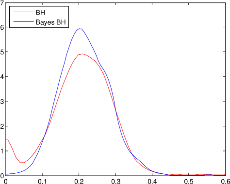
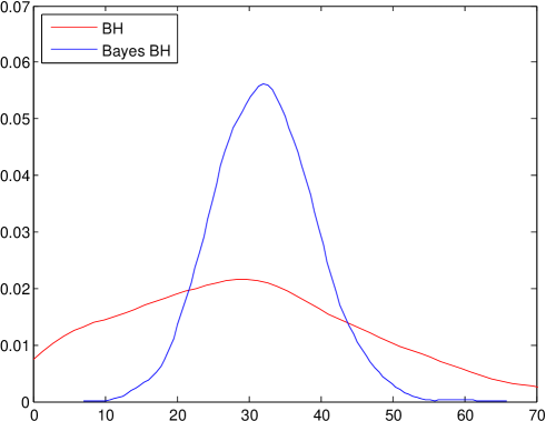
Figure 1: Densities of the $\mathrm{FDP}$ (left) and $\mathrm{NTD}$ (right) of the Bayes BH and BH procedures in the presence of strong dependence of hypotheses

$\psi=0.1$, $\alpha=0.2$, $\epsilon=1$, $\varrho_{2}=0.91$

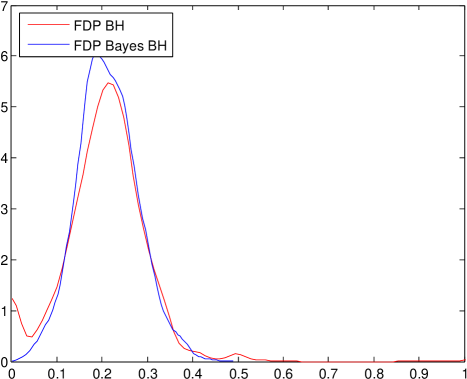
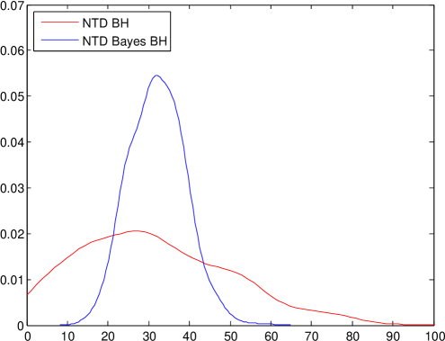
$\psi=0.1$, $\alpha=0.2$, $\epsilon=1$, $\varrho_{2}=0.96$

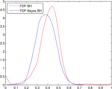
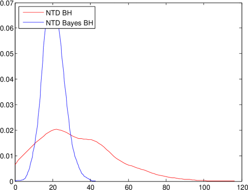
$\psi=0.05$, $\alpha=0.4$, $\epsilon=1$, $\varrho_{2}=0.95$

4.4.2 Additional effects of dependence structure on multiple testing

Table 3 displays the results of a set of simulations in which the dependence of the hypotheses is strong with $\varrho_{2}(\boldsymbol{P})=0.9591$. However, the third largest eigenmodulus, i.e. $\varrho_{3}(\boldsymbol{P})$, is also sampled to be relatively large at $0.5232$. This makes the sampling of $\boldsymbol{P}$ more difficult. In contrast, in the simulations of Section 4.4.1, there is no control on $\varrho_{3}(\boldsymbol{P})$ and as a result, $\varrho_{3}(\boldsymbol{P})$ is small. In most cases, the value is less than 0.3. For example, for the transition matrices in (16) and (17), the value of $\varrho_{3}(\boldsymbol{P})$ is 0.0645 and 0.1155, respectively. The transition matrix of the parent Markov chain for Table 3 is

$$\boldsymbol{P}=\begin{pmatrix}0.0014&0.9653&0.0124&0.0080&0.0129\\ 0.9506&0.0011&0.0056&0.0155&0.0272\\ 0.3236&0.1203&0.5312&0.0238&0.0011\\ 0.8080&0.1589&0.0190&0.0025&0.0115\\ 0.1898&0.7959&0.0053&0.0024&0.0066\\ \end{pmatrix}$$ (18)

with $\boldsymbol{\pi}=(0.47319,0.47681,0.018907,0.01173,0.019363)^{\mathrm{t}}$ and $\psi=0.05$. Note that the proportion of false nulls is only half as large as the one in Section 4.4.1, making error control more difficult. Table 3 shows that in this case, even though the Bayes BH procedure has a harder time to control the FDR, it has substantially less variation in the FDP than the BH procedure does. Further, the power of the Bayes BH procedure is clearly superior to the BH procedure. For example, at a realized FDP $\approx 0.35$, the former makes about 204 true discoveries whereas the latter makes about 149. The Bayes BH procedure also has significantly lower SE-to-mean ratio of the $\mathrm{NTD}$ than the BH procedure. The phenomenon was repeatedly observed when $\varrho_{3}(\boldsymbol{P})$ was sampled to be large. Figure 2 provides examples of the phenomenon. In contrast to Figure 1, the FDP density curves of the two procedures exhibit pronounced differences, and their NTD density curves are far apart instead of overlapping with each other.

Table 3: Comparison of the Bayes BH and BH procedures in the presence of strong dependence with large $\varrho_{2}$ and a relatively large $\varrho_{3}$. The transition matrix of the parent Markov chain is (18) with $\varrho_{2}=0.9591$, $\varrho_{3}>0.5$, and $\psi=5\%$.

		BBH	BH	BBH	BH
$\epsilon$	$\alpha$	$\hat{\mu}_{\mathrm{FDP}}$		$\mathrm{SE}(\hat{\mu}_{\mathrm{FDP}})$
1	0.2	0.29271	0.19	0.10223	0.23451
1	0.3	0.3676	0.30591	0.06527	0.19306
1	0.4	0.47105	0.40827	0.039127	0.11613
1.25	0.2	0.35611	0.1958	0.032559	0.086935
1.25	0.356	0.42145	0.35488	0.02103	0.041823
$\epsilon$	$\alpha$	$\hat{\mu}_{\mathrm{NTD}}$		$\mathrm{SE}(\hat{\mu}_{\mathrm{NTD}})$
1	0.2	23.739	9.0709	3.655	4.1191
1	0.3	53.006	13.288	11.094	9.1999
1	0.4	119.15	19.097	30.862	18.862
1.25	0.2	204.12	30.266	23.961	16.364
1.25	0.356	402.27	149.84	31.26	37.498

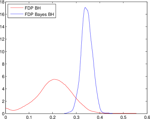
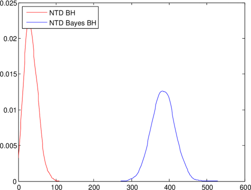
Figure 2: Densities of the $\mathrm{FDP}$ and $\mathrm{NTD}$ of the Bayes BH and BH procedures when both $\varrho_{2}$ and $\varrho_{3}$ are large

$\psi=0.05$, $\alpha=0.2$, $\epsilon=1.25$, $\varrho_{2}=0.91$, $\varrho_{3}=0.382$

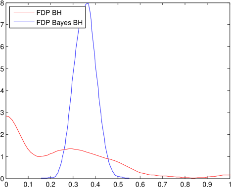
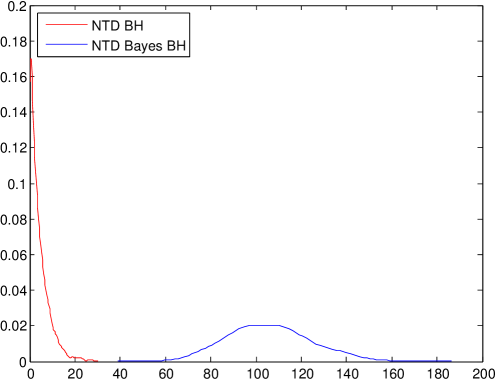
$\psi=0.05$, $\alpha=0.2$, $\epsilon=1$, $\varrho_{2}=0.904$, $\varrho_{3}=0.463$

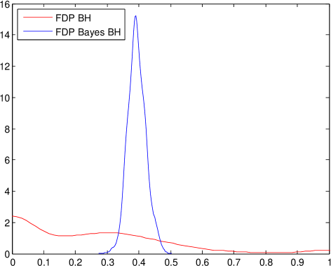
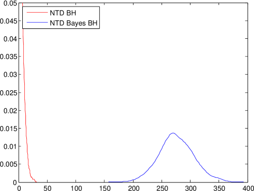
$\psi=0.05$, $\alpha=0.2$, $\epsilon=1$, $\varrho_{2}=0.904$, $\varrho_{3}=0.59$

As noted in the introduction, it is known that the BH procedure is often able to control the FDR under dependence, and certain properties of dependence are sufficient for this to happen [56, 3, 45, 46, 11]. Much less is known about the relationship between properties of dependence and other aspects of performance of multiple testing, such as stability and power. One advantage of random sampling from a large space of dependence structures is that it enables experimental investigation of the relationship. The properties of statistical dependence as characterized by $\varrho_{2}(\boldsymbol{P})$ and $\varrho_{3}(\boldsymbol{P})$ have been the focus here. The above results indicate that $\varrho_{2}(\boldsymbol{P})$ alone is not sufficient to characterize the relative performances of the Bayes BH and the BH procedures. This numerical observation is consistent with what is now known about the mixing times of Markov chains [12, 32]. The results in Table 3 and Figure 2 indicate that $\varrho_{3}(\boldsymbol{P})$ may sometimes play a role in shaping the differences. In our simulations, $\boldsymbol{P}$ is a $5\times 5$ matrix. Thus $\varrho_{2}(\boldsymbol{P})$ and $\varrho_{3}(\boldsymbol{P})$ together provide a significant part of information on the spectrum of the transition matrix. This points to a complex relationship between the dependence structure of the underlying hypotheses and the relative performances of the Bayes BH and the BH procedures.

4.4.3 Moderate dependence

Table 4 displays results for the case of moderate dependence. In this set of simulations, $\varrho_{2}(\boldsymbol{P})=0.6019$,

$$\boldsymbol{P}=\begin{pmatrix}0.1999&0.6548&0.0537&0.0561&0.0354\\ 0.8932&0.0765&0.0137&0.0088&0.0076\\ 0.4431&0.4365&0.0721&0.0284&0.0199\\ 0.1159&0.8271&0.0371&0.0129&0.0070\\ 0.6080&0.0597&0.0505&0.0710&0.2108\\ \end{pmatrix}$$ (19)

with $\boldsymbol{\pi}=(0.4969,0.4031,0.0376,0.0349,0.0275)^{\mathrm{t}}$ and $\psi=0.1$. From the table, the $\mathrm{NTD}$ of the Bayes BH procedure is clearly more stable than that of the BH procedure. This can also be seen from the densities of the $\mathrm{NTD}$ shown in Figure 3. To a lesser extent, the $\mathrm{FDP}$ of the Bayes BH procedure is also more stable than that of the BH procedure except when $\epsilon=0.75$, $\alpha=0.3$ or $0.4$. In the latter situation, the variance of the $\mathrm{FDP}$ of the Bayes BH procedure is still competitive with that of the BH procedure.

Table 4: Comparison of the Bayes BH and BH procedures in the presence of moderate dependence. The transition matrix of the parent Markov chain is (19) with $\varrho_{2}=0.6019$ and $\psi=10\%$

		BBH	BH	BBH	BH
$\epsilon$	$\alpha$	$\hat{\mu}_{\mathrm{FDP}}$		$\mathrm{SE}(\hat{\mu}_{\mathrm{FDP}})$
0.75	0.3	0.29201	0.3071	0.20283	0.20708
0.75	0.4	0.22492	0.3014	0.2719	0.2124
0.75	0.5	0.4966	0.50118	0.03134	0.045887
1	0.2	0.192	0.2012	0.075112	0.084956
1	0.3	0.294	0.30074	0.035074	0.040486
$\epsilon$	$\alpha$	$\hat{\mu}_{\mathrm{NTD}}$		$\mathrm{SE}(\hat{\mu}_{\mathrm{NTD}})$
0.75	0.3	2.094	9.431	1.8608	9.2073
0.75	0.4	22.28	38.658	5.6593	25.412
0.75	0.5	121.26	138.26	12.793	60.366
1	0.2	22.542	32.796	5.8157	18.614
1	0.3	116.64	129.34	12.984	42.037

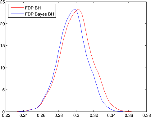
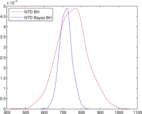
Figure 3: Densities of the FDP and NTD of the Bayes BH and BH procedures in the presence of moderate dependence of hypotheses

$\psi=0.1$, $\alpha=0.3$, $\epsilon=1.25$, $\varrho_{2}=0.67$

4.4.4 Independence

Finally, as a test on the validity of the Bayes BH procedure, Table 5 displays results when $\varrho_{2}(\boldsymbol{P})=0$ and, as a result, the entries of $\boldsymbol{\eta}$ are i.i.d. In the simulations, $\psi=0.05$ and $\boldsymbol{P}=\boldsymbol{1}_{5}\boldsymbol{\pi}^{\mathrm{t}}$, where the stationary probability vector $\boldsymbol{\pi}$ is randomly sampled as in Section 4.1. As can be seen, under independence, both the Bayes BH procedure and the BH procedure are valid. In terms of power, although the NTD of the Bayes BH procedure has a smaller average than that of the BH procedure, its stability is clearly superior. Similar phenomenon can be seen from the density plot in Figure 3.

Table 5: Comparison of the Bayes BH and BH procedures when there is no dependence in data

		BBH	BH	BBH	BH
$\epsilon$	$\alpha$	$\hat{\mu}_{\mathrm{FDP}}$		$\mathrm{SE}(\hat{\mu}_{\mathrm{FDP}})$
1	0.3	0.29028	0.29932	0.19437	0.18847
1	0.4	0.39102	0.39308	0.081393	0.123
1	0.5	0.50282	0.50157	0.039488	0.065857
1.25	0.2	0.19442	0.19951	0.072535	0.083292
$\epsilon$	$\alpha$	$\hat{\mu}_{\mathrm{NTD}}$		$\mathrm{SE}(\hat{\mu}_{\mathrm{NTD}})$
1	0.3	5.322	11.16	2.9969	9.6522
1	0.4	22.881	32.613	5.9599	19.899
1	0.5	79.951	87.779	10.701	36.661
1.25	0.2	24.838	31.121	5.9329	15.893

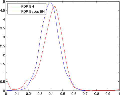
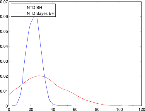
Figure 4: Densities of the FDP and NTD of the Bayes BH and BH procedures when hypotheses are independent

$\psi=0.05$, $\alpha=0.4$, $\epsilon=1$, $\varrho_{2}=0$

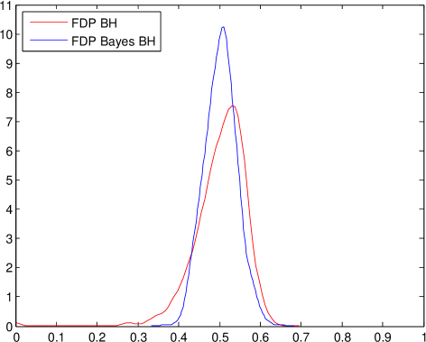
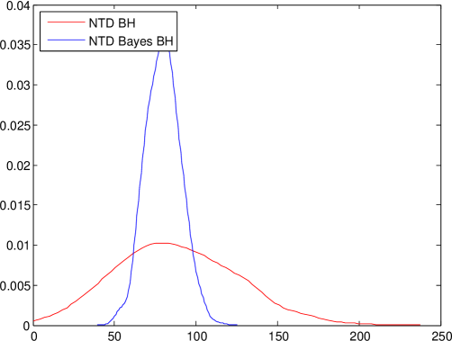
$\psi=0.05$, $\alpha=0.5$, $\epsilon=1$, $\varrho_{2}=0$

5 Conclusion

We presented a flexible signal processing model of large scale multiple testing and used probability approximation to conduct multiple testing. This allowed us to empirically demonstrate that even when very little is known about the dependence structure of the hypotheses, substantial reduction in variance can be achieved by using approximated conditional probabilities in multiple testing. Using simulations designed to generate very general dependence structures, we provided evidence for the effectiveness of the local conditioning approach to FDR and power variance reduction in large scale multiple testing. Conditional likelihood has been fruitfully exploited in multiple testing [18, 15, 16]. Indeed, the notion of Local False Discovery Rate introduced in [18] is a conditional likelihood that does not directly borrow strength from nearby observations. In contrast, our approach explicitly incorporates nearby observations into the conditional likelihood. Our analysis indicates that the reduction in the standard deviations of the FDP and the number of true discoveries can be substantial when conditional likelihood is used. In particular, for very noisy data, even when there is some increase in the FDR as compared to using $p$-values the reduction in the standard deviation of FDR may justify a Bayesian approach.

The effects of dependence on large scale multiple tests has been a topic of research at least since the beginning of this century [3]. Various special dependence structures between the hypotheses have been studied and continue to be studied to ascertain the effectiveness of both $p$-value based and Empirical Bayes methods [3, 56, 53] in multiple testing. In addition, with some notable exceptions [39, 21, 40, 49, 26, 33], the standard deviations of the FDR and the number of true discoveries has usually taken a second place to the estimates themselves. However, given that it is often impractical to repeat a multiple test numerous times, not controlling the standard deviation of the power and the FDR can lead to highly biased estimates of FDR. The need for simulating general dependence structures is crucial to testing the performance of our approach. This led us to the random HMM dependence structures that can be generated by using random Markov matrices using Sinkhorn’s algorithm.

Our approach strikes a compromise between generality and tractability by using the signal processing framework that models data as a function of signal, signal strength, i.i.d. noise and signal noise interaction. The flexibility can be useful in application. For instance, additive noise is not the only signal-noise interaction that is seen in fMRI practice [37], so a different signal-noise interaction function may improve the analysis. Assuming a fixed signal noise interaction and a fixed noise distribution is not unrealistic in many applications. The challenge is that they are usually unknown. Two important issues that we have not addressed here is modeling real data with this approach and obtaining a “noiseless” sample of the data for measuring moments. These two issues are intimately connected to the application in question. Obtaining a noiseless sample of the signals is not very difficult in a signal processing context. However, in DNA microarray analysis and in fMRI it remains a challenge to not just find a noiseless sample but also to arrive at the signal strength and the signal noise interaction. A possible solution might be to incorporate a parametric model to the underlying binary process that identifies false nulls. Thus our next goal is the development of ideas that successfully apply the signal processing and local dependence approach to multiple testing.

The connection of large scale multiple testing to signal processing is obvious but the challenge in applications is often that very little is known about the signal distribution, signal dependence, the noise distribution and how they interact. However this is not always the case [lindquist_2008, 34]. Stochastic models of fMRI data have been modeled in the signal processing framework using random fields [48, 9]. The fMRI blood-oxygen-level dependent (BOLD) response is the signal of interest. Multiple types of noise including system-related instabilities, subject motion and physiological fluctuation corrupt the signal [lindquist_2008]. The “signal-to-noise-ratio” captures the signal strength; see Figure 5 in [34].

We have developed a novel flexible stochastic modeling framework for casting an arbitrary multiple test as a signal processing problem. It explicitly decomposes the data into four distinct inputs. A Bernoulli signal process or network, a noise with an arbitrary continuous distribution, a scalar signal strength and a signal-noise interaction function. Each of these features is relevant to fMRI data. We place very few assumptions on the dependence structure of the signals while allowing local correlation. Our probality model allows an arbitrary, but known, continuous noise distribution. Our model allows an arbitrary, but known, signal-noise interaction function.

References

- [1] Barvinok, A. (2010). What does a random contingency table look like? Combin. Probab. Comput. 19, 4, 517–539.
- [2] Benjamini, Y. and Hochberg, Y. (1995). Controlling the false discovery rate: a practical and powerful approach to multiple testing. J. R. Stat. Soc. Ser. B 57, 289–300.
- [3] Benjamini, Y. and Yekutieli, D. (2001). The control of the false discovery rate in multiple testing under dependency. Ann. Statist. 29, 4, 1165–1188.
- [4] Bordenave, C., Caputo, P., and Chafaï, D. (2012). Circular law theorem for random Markov matrices. Probab. Theory Related Fields 152, 3–4, 751–779.
- [5] Brualdi, R. A., Parter, S. V., and Schneider, H. (1966). The diagonal equivalence of a nonnegative matrix to a stochastic matrix. J. Math. Anal. Appl. 16, 31–50.
- [6] Cappellini, V., Sommers, H.-J., Bruzda, W., and Życzkowski, K. (2009). Random bistochastic matrices. J. Phys. A 42, 36, 365209, 23 pp.
- [7] Chafaï, D. (2010). The Dirichlet Markov ensemble. J. Multivariate Anal. 101, 3, 555–567.
- [8] Chatterje, S., Diaconis, P., and Sly, A. (2010). Properties of uniform doubly stochastic matrices. ArXiv e-prints..
- [9] Cheng, D. and Schwartzman, A. (2017). Multiple testing of local maxima for detection of peaks in random fields. Ann. Statist. 45, 2, 529–556.
- [10] Chi, Z. (2011). Effects of statistical dependence on multiple testing under a hidden Markov model. Ann. Statist. 39, 1, 439–473.
- [11] Clarke, S. and Hall, P. (2009). Robustness of multiple testing procedures against dependence. Ann. Statist. 37, 1, 332–358.
- [12] Diaconis, P. (1995). The cutoff phenomenon in finite Markov chains. Proc. Natl. Acad. Sci. USA 93, 1659––1664.
- [13] Diaconis, P., Lebeau, G., and Michel, L. (2012). Gibbs/Metropolis algorithms on a convex polytope. Math. Z. 272, 1-2, 109–129.
- [14] Eaves, B. C., Hoffman, A. J., Rothblum, U. G., and Schneider, H. (1985). Line-sum-symmetric scalings of square nonnegative matrices. Math. Programming Stud. 25, 124–141. Mathematical programming, II.
- [15] Efron, B. (2004). Large-scale simultaneous hypothesis testing: the choice of a null hypothesis. J. Amer. Statist. Assoc. 99, 465, 96–104.
- [16] Efron, B. (2007). Correlation and large-scale simultaneous significance testing. J. Amer. Statist. Assoc. 102, 477, 93–103.
- [17] Efron, B. (2010). Correlated -values and the accuracy of large-scale statistical estimates. J. Amer. Statist. Assoc. 105, 491, 1042–1055.
- [18] Efron, B., Tibshirani, R., Storey, J. D., and Tusher, V. G. (2001). Empirical Bayes analysis of a microarray experiment. J. Amer. Statist. Assoc. 96, 456, 1151–1160.
- [19] Eklund, A., Nichols, T. E., and Knutsson, H. (2016). Cluster failure: why hy fMRI inferences for spatial extent have inflated false-positive rates. Proc. Natl. Acad. Sci. USA 113, 28, 7900–7905.
- [20] Fan, J. and Han, X. (2017). Estimation of the false discovery proportion with unknown dependence. J. R. Stat. Soc. Ser. B 79, 4, 1143–1164.
- [21] Fan, J., Han, X., and Gu, W. (2012). Estimating false discovery proportion under arbitrary covariance dependence. J. Amer. Statist. Assoc. 107, 499, 1019–1035.
- [22] Farcomeni, A. (2008). A review of modern multiple hypothesis testing, with particular attention to the false discovery proportion. Stat. Methods Med. Res. 17, 4, 347–388.
- [23] Franklin, J. and Lorenz, J. (1989). On the scaling of multidimensional matrices. Linear Algebra Appl. 114/115, 717–735.
- [24] Genovese, C. and Wasserman, L. (2004). A stochastic process approach to false discovery control. Ann. Statist. 32, 3, 1035–1061.
- [25] Goldberg, G. and Neumann, M. (2003). Distribution of subdominant eigenvalues of matrices with random rows. SIAM J. Matrix Anal. Appl. 24, 3, 747–761 (electronic).
- [26] Gordon, A., Glazko, G., Qiu, X., and Yakovlev, A. (2007). Control of the mean number of false discoveries, Bonferroni and stability of multiple testing. Ann. Appl. Statist. 1, 1, 179–190.
- [27] Hartfiel, D. J. (1971). Concerning diagonal similarity of irreducible matrices. Proc. Amer. Math. Soc. 30, 419–425.
- [28] Hartfiel, D. J. (1974). A study of convex sets of stochastic matrices induced by probability vectors. Pacific J. Math. 52, 405–418.
- [29] Knight, P. A. (2008). The Sinkhorn-Knopp algorithm: convergence and applications. SIAM J. Matrix Anal. Appl. 30, 1, 261–275.
- [30] Künsch, H., Geman, S., and Kehagias, A. (1995). Hidden Markov random fields. Ann. Appl. Probab. 5, 3, 577–602.
- [31] Leek, J. T. and Storey, J. D. (2008). A general framework for multiple testing dependence. Proc. Natl. Acad. Sci. USA 105, 48, 18718––18723.
- [32] Levin, D. A., Peres, Y., and Wilmer, E. L. (2009). Markov chains and mixing times. American Mathematical Society, Providence, RI. With a chapter by James G. Propp and David B. Wilson.
- [33] Li, D. (2015). Power and stability comparisons of multiple testing procedures with false discovery rate control. Journal of Statistical Computation and Simulation 85, 14, 2808–2822.
- [34] Lindquist, M. A. and Mejia, A. (2015). Zen and the art of multiple comparisons. Psychosom. Med. 77, 2, 114–125.
- [35] Liu, J., Zhang, C., and Page, D. (2016). Multiple testing under dependence via graphical models. Ann. Appl. Stat. 10, 3, 1699–1724.
- [36] Marshall, A. W. and Olkin, I. (1968). Scaling of matrices to achieve specified row and column sums. Numer. Math. 12, 83–90.
- [37] Marx, M., Pauly, K. B., and Chang, C. (2013). A novel approach for global noise reduction in resting-state fMRI: APPLECOR. Neuroimage 64, 19–31.
- [38] Nguyen, H. D., McLachlan, G. J., Cherbuin, N., and Janke, A. L. (2014). False discovery rate control in magnetic resonance imaging studies via Markov random fields. IEEE Trans Med Imaging 33, 8, 1735–1748.
- [39] Owen, A. B. (2005). Variance of the number of false discoveries. J. R. Stat. Soc. Ser. B 67, 3, 411–426.
- [40] Qiu, X., Klebanov, L., and Yakovlev, A. (2005). Correlation between gene expression levels and limitations of the empirical Bayes methodology for finding differentially expressed genes. Stat. Appl. Genet. Mol. Biol. 4, Art. 34, 32 pp. (electronic).
- [41] Roquain, E. (2011). Type I error rate control for testing many hypotheses: a survey with proofs. Journal de la Societe Francaise de Statistique 152, 2, 3–38.
- [42] Roquain, E. and Villers, F. (2011). Exact calculations for false discovery proportion with application to least favorable configurations. Ann. Statist. 39, 1, 584–612.
- [43] Rosenthal, J. S. (1995). Convergence rates for Markov chains. SIAM Rev. 37, 3, 387–405.
- [44] Rothblum, U. G. and Schneider, H. (1989). Scalings of matrices which have prespecified row sums and column sums via optimization. Linear Algebra Appl. 114/115, 737–764.
- [45] Sarkar, S. K. (2002). Some results on false discovery rate in stepwise multiple testing procedures. Ann. Statist. 30, 1, 239–257.
- [46] Sarkar, S. K. (2006). False discovery and false non-discovery rates in single-step multiple testing procedures. Ann. Statist. 34, 1, 394–415.
- [47] Sarkar, S. K., Zhou, T., and Ghosh, D. (2008). A general decision theoretic formulation of procedures controlling FDR and FNR from a Bayesian perspective. Statistica Sinica 18, 925–945.
- [48] Schwartzman, A., Gavrilov, Y., and Adler, R. J. (2011). Multiple testing of local maxima for detection of peaks in 1D. Ann. Statist. 39, 6, 3290–3319.
- [49] Schwartzman, A. and Lin, X. (2011). The effect of correlation in false discovery rate estimation. Biometrika 98, 1, 199–214.
- [50] Simes, R. J. (1986). An improved Bonferroni procedure for multiple tests of significance. Biometrika 73, 3, 751–754.
- [51] Sinkhorn, R. (1964). A relationship between arbitrary positive matrices and doubly stochastic matrices. Ann. Math. Statist. 35, 876–879.
- [52] Sinkhorn, R. (1967). Diagonal equivalence to matrices with prescribed row and column sums. Amer. Math. Monthly 74, 402–405.
- [53] Stephens, M. (2017). False discovery rates: a new deal. Biostatistics 18, 2, 275–294.
- [54] Storey, J. D., Taylor, J. E., and Siegmund, D. O. (2004). Strong control, conservative point estimation and simultaneous conservative consistency of false discovery rates: a unified approach. J. R. Stat. Soc. Ser. B 66, 1, 187–205.
- [55] Sun, W. and Cai, T. T. (2009). Large-scale multiple testing under dependence. J. R. Stat. Soc. Ser. B 71, 2, 393–424.
- [56] Wu, W.-B. (2008). On false discovery control under dependence. Ann. Statist. 36, 1, 364–380.