How rare is the Bullet Cluster
(in a $\Lambda$CDM universe)?

Abstract

The Bullet Cluster (1E 0657-56) is well-known as providing visual evidence of dark matter but it is potentially incompatible with the standard $\Lambda$CDM cosmology due to the high relative velocity of the two colliding clusters. Previous studies have focussed on the probability of such a high relative velocity amongst selected candidate systems. This notion of ‘probability’ is however difficult to interpret and can lead to paradoxical results. Instead, we consider the expected number of Bullet-like systems on the sky up to a specified redshift, which allows for direct comparison with observations. Using a Hubble volume N-body simulation with high resolution we investigate how the number of such systems depends on the masses of the halo pairs, their separation, and collisional angle. This enables us to extract an approximate formula for the expected number of halo-halo collisions given specific collisional parameters. We use extreme value statistics to analyse the tail of the pairwise velocity distribution and demonstrate that it is fatter than the previously assumed Gaussian form. We estimate that the number of dark matter halo pairs as or more extreme than 1E 0657-56 in mass, separation and relative velocity is $1.3^{+2.0}_{-0.6}$ up to redshift $z=0.3$. However requiring the halos to have collided and passed through each other as is observed decreases this number to only 0.1. The discovery of more such systems would thus indeed present a challenge to the standard cosmology.

1 Introduction

Large clusters of galaxies are the biggest gravitationally bound objects in the universe. Naïvely they would be expected to correspond to ‘fundamental observers’ who follow the Hubble flow and move away from each other. The discovery of the Bullet Cluster (1E 0657-56), a system consisting of two very massive clusters of galaxies which have undergone a collision with a high relative velocity, thus requires an assessment of whether the standard $\Lambda$CDM cosmology is able to accommodate such an extreme event. The subsequent discovery of many more merging clusters motivates a general study of the statistics of such events. Since such collisions involve non-linear interactions, the predictions of the $\Lambda$CDM model have to be extracted from cosmological N-body simulations.

The Bullet Cluster located at $z=0.296$ is the best studied of such mergers, since its collisional trajectory is normal to the line of sight. It is extreme in several respects. The main cluster has a high mass of $M_{\rm main}\simeq 1.5\times 10^{15}M_{\odot}$, with the subcluster mass $M_{\rm Bullet}\simeq 1.5\times 10^{14}M_{\odot}$, separation $d_{12}\simeq 0.72$ Mpc [1, 2], and a very high velocity $v_{12}\simeq 4500$ km/s [3] deduced from the analysis of the bow shock. This should be compared to the expected separation velocity in the Hubble flow: $v_{\rm Hubble}=H_{z=0.3}\times d_{12}\simeq 70$ km/s, where $H_{z}\simeq H_{0}(1+z)\sqrt{1+\Omega_{m}z}$ and $H_{0}\equiv 100h$  km/s/Mpc is the Hubble parameter at $z=0$ with $h\simeq 0.7$. However the relative velocity of the two dark matter (DM) peaks does not necessarily correspond to the shock front velocity of the baryons observed in X-rays, and a lower estimate of $v_{12}\simeq 3000$ km/s was given in Ref.[4].

Recent hydrodynamical simulations indeed show that the morphology (DM and gas) of the Bullet system is well reproduced by requiring $v_{12}\simeq 3000$ km/s and $d_{12}\simeq 2.5$ Mpc/$h$ between the DM halos at redshift $z=0.5$ [5, 6]. This is broadly comparable to Ref.[7] which had estimated earlier: $v_{12}\simeq 3200$ km/s at $d_{12}\simeq 2.5$ Mpc/$h$. Simpler hydrodynamical simulations done earlier [8, 9] had also found a lower relative velocity to reproduce the morphology better. The extreme properties of 1E 0657-56 can now be framed in terms of these initial conditions required to produce the observed collision.

Searching for Bullet-like systems satisfying these initial conditions in N-Body simulations is convenient as the two clusters can be taken to be well separated and are thus easily identified. However because of its rarity the Bullet system can only be found in the largest N-Body simulations, provided the mass resolution is good (i.e. the DM ‘particle’ mass is small). Ref.[10] shows that to find a Bullet-like system, the volume of the simulation needs to be at least $\sim(4.5$ Gpc/$h)^{3}$, with the mass resolution better than $M_{\rm par}\sim 6.5\times 10^{11}M_{\odot}/h$.

Various definitions of what constitutes a Bullet-like system have been employed. Ref.[11] used a 0.5 (Gpc/$h$)³ simulation and looked at the most massive subclusters moving away from the host cluster with velocity $>4500$ km/s and a separation $>0.7$ Mpc/$h$ at redshift $z=0.3$. With such a small simulation volume they did not find any host halo as massive as 1E 0657-56 so needed to extrapolate to find the fraction of appropriate subclusters. They estimated this to be $\sim 0.01$, however this is uncertain to at least an order of magnitude.

Ref.[12] used a (3 Gpc/$h)^{3}$ simulation with $M_{\rm par}\sim 2.3\times 10^{11}M_{\odot}/h$ to look at the fraction of subhalos with high enough velocity among systems satisfying the conditions in Ref.[7]. This fraction, dubbed ‘probability’, was found to be about $10^{-10}$ at $z=0$, by fitting a Gaussian to the pairwise velocity distribution in order to estimate the tail of the distribution. This was interpreted as an inconsistency between $\Lambda$CDM and the observation of 1E 0657-56.

Ref.[10] studied the effect of the box size and the resolution on the tail of the pairwise velocity distribution and found that simulations with small boxes and poor resolution struggle to produce systems as extreme as 1E 0657-56. Using rather different definitions for a Bullet-like system than Refs.[11] and [12] they estimated the fraction of systems with high enough relative velocity by fitting a skewed Gaussian to the pairwise velocity distribution. Again dubbed ‘probability’, this was estimated to be $\sim 10^{-8}$, still very inconsistent with $\Lambda$CDM.

Ref.[13] used a large simulation with volume of (21 Gpc/$h)^{3}$ but poor resolution $M_{\rm par}\sim 1.2\times 10^{12}M_{\odot}/h$. They also used a different percolation parameter ($b=0.15$ instead of the conventional $b=0.2$) in their Friend of Friends (FoF) halo finder, arguing that this more faithfully reconstructs the masses of halos corresponding to the Bullet system. The tail of the pairwise velocity distribution was analysed in the Extreme Value Statistics (EVS) approach to show that it is significantly fatter than a Gaussian-like tail. Using a similar definition for Bullet-like systems as Ref.[10] they found that the fraction (again called ‘probability’) of such high-velocity encounters is about $\sim 6\times 10^{-6}$, again raising a problem for $\Lambda$CDM.

Ref.[14] explored the effect of halo finders on the pairwise velocity distribution. In particular, a configuration-space based FoF algorithm was compared to rockstar [15], a phase-space based halo finder. Using the same definition for a Bullet-like system as in Ref.[10], it was found that the FoF halo finder fails to identify the collisions in the high-velocity tail and leads to ‘probabilities’ almost two orders of magnitude lower that when the better performing rockstar halo finder is used.

Finally Ref.[16] used a (6 Gpc/$h)^{3}$ volume with $M_{\rm par}\sim 7.5\times 10^{11}M_{\odot}/h$ and argued that a Bullet-like system [8] at $z=0.3$ is not too far from other halo pairs in the simulation. Instead of focussing on the extreme properties of colliding dark matter halos, Ref.[17] looked at the morphology of the gas and dark matter in the colliding clusters and found that the displacement between the gas and dark matter similar to 1E 0657-56 is expected in about 1% of the clusters. Some other investigations [4, 13, 18] have even considered whether the apparent inconsistency posed by the Bullet Cluster can be alleviated by invoking a new long range ‘fifth’ force in the ‘dark sector’. Rather than engage in such speculations we address in this paper the main shortcoming of the previous studies, viz. the ill-defined ‘probability’ of finding systems like 1E 0657-56 on the sky.

We use Dark Sky Simulations [19], one of the biggest N-Body simulations with volume (8 Gpc/$h)^{3}$, as well as one of the best resolutions $M_{\rm par}\sim 3.9\times 10^{10}M_{\odot}/h$. The halo catalogue used was produced by a phase-space based (rockstar) halo finder that performs better than the configuration-space based finders used earlier. We carefully explore the dependence of the pairwise velocity distribution on the different definitions of Bullet-like systems. Furthermore, the machinery of EVS is used to examine the tail of the distribution, rather than assuming that a Gaussian fit is a good description. We also study an observationally better motivated quantity, viz. the absolute number of bullet-like systems expected in a survey up to some particular redshift. This should be contrasted with the fraction of extreme objects (in a population of less extreme objects) that has been the focus of earlier studies.

In Section 2 we describe the N-Body simulation used and demonstrate the importance of using a phase-space based halo finder for searching for systems similar to 1E 0657-56. Section 3 summarises the EVS tools relevant for modelling the tails of distributions. In Section 4 we show how the expected number of Bullet-like systems can be estimated. We also discuss some of the paradoxical features of the ‘probability’ — defined as a fraction of Bullet-like systems in a population of candidate systems — that has been studied previously. Section 5 contains the main results of our paper, viz. the expected number of systems similar to 1E 0657-56 in $\Lambda$CDM.

2 Simulations and halo finders

The biggest dataset of the Dark Sky Simulation (DS) Early Data Release [19] has a box of volume (8 Gpc/$h)^{3}$ with $N^{3}=10240^{3}$ ‘dark matter particles’ corresponding to $M_{\rm par}\sim 3.9\times 10^{10}M_{\odot}/h$. Such a large volume and good resolution make it ideal for the study of rare objects like the Bullet Cluster [10].

Halos in the DS simulation were identified with the rockstar [15] halo finder. For computational convenience we reduced the halo catalogue by requiring $M_{\rm halo}>3.5\times 10^{13}M_{\odot}/h$. rockstar is a phase-space based halo finder and therefore performs better at identifying Bullet-like systems which are characterised by a small distance between the two massive clusters with a high relative velocity. Standard Friend of Friend (FoF) halo finders work in configuration space and therefore struggle to tell the two nearby clusters apart — this leads to underestimation of the number of Bullet-like systems in N-Body simulations. In phase space however the host and the bullet clusters are well separated due to the high relative velocity, hence can be correctly identified as two separate clusters.

To illustrate this point, the host and the bullet halo are generated at the DS simulation resolution, using the NFW [20] density profile as it best fits weak lensing data on 1E 0657-56 [4]. The DM particles are given the velocities as in Ref.[21]. The two halos are placed at various distances with their relative velocity set at 3000 km/s. Then both rockstar and a FoF algorithm with percolation parameter $b=0.2$ are used to extract the halo information. At separations of 5 Mpc/$h$ and 4 Mpc/$h$ both halo finders identify the two halos correctly. However at 3 Mpc/$h$ the FoF algorithm identifies 2 halos only $\sim$30% of the time, while at 2 Mpc/$h$ and below it identifies only 1. By contrast, rockstar finds 2 halos at all separations. Thus we expect a depletion of the number of nearby mergers when a FoF based halo finder is used, leading to underestimation of the number of objects similar to the Bullet system.

3 Extreme value statistics

Events in the tail of the pairwise velocity distribution need to be modelled without assuming a functional form for the underlying distribution and EVS provides a framework for doing so. We briefly outline the formalism relevant to this study following Ref.[22].

We are interested in modelling the statistical behaviour of extreme values of a random variable $X$. The probability that $X$ exceeds a specified high threshold $\mu$ is:

$${\rm Pr}\left\{X>\mu+x|X>\mu\right\}=\frac{1-F(\mu+x)}{1-F(\mu)}$$ (3.1)

Here $F(x)={\rm Pr}\left\{X<x\right\}$ is the cumulative distribution function which is unknown and needs to be estimated.

The central result of EVS is that the maxima of a sequence of random variables $X_{\rm max}=\left\{X_{1},...,X_{N}\right\}$ with a common cumulative distribution function $F(x)$ tend to be distributed in the limit $N\rightarrow\infty$ according the Generalized Extreme Value distribution $G(x)$:

$${\rm Pr}\left\{X_{\rm max}<x\right\}=F_{X_{1}}(x)\times...\times F_{X_{N}}(x)=F^{N}(x)\approx G(x)$$ (3.2)

where

$$G_{\mu,\sigma,\xi}(x)=\exp\left\{-\left[1+\xi\left(\frac{x-\mu}{\sigma}\right)\right]^{-1/\xi}\right\}$$ (3.3)

for some $\mu,\sigma>0$ and $\xi$. From Eqs.(3.2) and (3.3) we can estimate $F(x)$ and thus approximate Eq.(3.1) by the Generalized Pareto Distribution (GPD) $H(x)$:

$${\rm Pr}\left\{X>\mu+x|X>\mu\right\}=1-H_{\mu,\sigma,\xi}(x),\quad\mathrm{where:} H_{\mu,\sigma,\xi}(x)=1-\left[1+\xi\left(\frac{x-\mu}{\sigma}\right)\right]^{-1/\xi}$$ (3.4)

with the condition $1+\xi\left((x-\mu)/\sigma\right)>0$. The above expression is fitted to the extreme events and provides a model independent description of the tails of probability distributions. If the underlying distribution is ‘Gaussian-like’ (e.g. Gaussian or skewed Gaussian), the tail parameter $\xi$ equals 0. Longer tails have $\xi>0$ whereas shorter ones have $\xi<0$.

The next step in modelling the tail is the choice of the threshold $\mu$. If it is too low, the asymptotically valid GPD does not apply and our estimate will be biased. If $\mu$ is too high, the reduced number of extreme events available results in high variance in the estimated parameters. Provided the GPD description is valid above some threshold $\mu_{1}$ then it is also valid for a higher threshold $\mu_{2}>\mu_{1}$ with new parameters ($\mu_{2},\sigma_{\mu_{2}},\xi_{\mu_{2}}$). However, the tail parameter $\xi_{\mu}$ and the combination $\sigma_{\mu}-\mu\xi_{\mu}$ should remain constant. Therefore the simplest method for the appropriate choice of the threshold $\mu$ focusses on finding a region of stability of these parameter combinations. In order to minimise the variance, the lowest $\mu$ consistent with stability is finally chosen as the threshold.

4 The number (versus ‘probability’) of Bullet-like systems

A Bullet-like system can be defined by cuts in the collisional parameters describing the merger of two clusters. Such a definition is particularly suited for the DM-only N-Body simulations. The collisional parameters are the separation $d_{12}$ between the two halos, the two masses $m_{1}$ and $m_{2}$, the relative speed $v_{12}$, and the angle $\theta$ between the relative velocity and the separation. To simplify the problem the mass cut is often made in terms of the average mass $\langle M\rangle$ of the two halos and we shall do so too.

The most prominent feature of 1E 0657-56 is the high relative velocity of its subcluster with respect to the main cluster. Thus both the pairwise velocity distribution $\mathrm{d}n/\mathrm{d}v_{12}$ and its cumulative $n(>v_{12})$ (where $n$ is the number density of the halo pairs) will be studied.

The observationally relevant quantity is the expected number of Bullet-like objects up to some redshift. However, the quantity studied so far has been the fraction of such objects with respect to less extreme candidate systems (i.e. having a lower relative velocity) [11, 14, 13, 10, 12]. This fraction is then interpreted as the ‘probability’ of finding a Bullet-like system although it is not directly related to the likelihood of observing such an object on the sky. In terms of the number densities it is expressed as $p_{v}=n(v_{12}>v_{\rm Bullet}\mid\textrm{other cuts})/n(v_{12}>0\mid\textrm{other cuts})$. The probability defined in this way is relative to the objects defined by the initial mass, distance, and angle cuts and has a non-trivial and sometimes paradoxical dependence on those cuts. For example, increasing the mass cut in the definition of a Bullet-like system leads to an increase in the ‘probability’, even though the actual number of systems has been reduced drastically (see Figs. 2-3).

Alternatively, the high masses of the two colliding clusters can be taken as the main defining parameters and the ‘probability’ written as $p_{m}=n(m_{1},m_{2}>M_{\rm main},M_{\rm Bullet}\mid\textrm{other cuts})/n(m_{1},m_{2}>0\mid\textrm{other cuts})$, where the relative velocity cut has now been taken before the mass cut. Even though we are looking at the same Bullet-like objects, one finds $p_{v}\neq p_{m}$ simply due to the different order of the cuts taken in the collisional parameters.

In what follows we focus therefore on the observationally motivated and intuitively accessible quantity, viz. the expected number of Bullet-like systems on the sky up to a specified redshift. This can be expressed (in a flat universe) as:

$$N(<z)=\int_{0}^{z}n(v_{12}>v_{\rm Bullet},\mathrm{cuts}\mid z^{\prime})4\pi D_{\rm c}^{2}(z^{\prime})\,\mathrm{d}D_{\rm c}(z^{\prime}),$$ (4.1)

where $n(v_{12}>v_{\rm Bullet},\mathrm{cuts}\mid z)$ is the comoving number density of Bullet-like objects at redshift $z$, and $D_{\rm c}(z)$ is the comoving distance to $z$.

Estimating the pairwise velocity function $\mathrm{d}n/\mathrm{d}v_{12}$ and its cumulative version $n(>v_{12})$ in large simulations at many different redshifts can be computationally expensive. However, $\mathrm{d}n/\mathrm{d}v_{12}$, and consequently $n(>v_{12})$, were found to have a stable shape up to $z\sim 0.5$ [13, 10]. This simplifies the analysis and we can approximate:

$$n(v_{12}>v_{\rm Bullet},\mathrm{cuts}\mid z)\approx\alpha(z)\times n(v_{12}>v_{\rm Bullet},\mathrm{cuts}\mid z=0),$$ (4.2)

where the normalisation $\alpha(z)$ is proportional to the number of pairs of halos satisfying specific cuts (mass, distance …) and is set equal to 1 at $z=0$. When one halo has a mass above $m_{1}$ and the other above $m_{2}$, with their separation less than $d_{12}$, it can be written as:

$$\alpha(z)\propto\iiint\limits_{m_{1},m_{2},0}^{~{}~{}~{}\infty,\infty,d_{12}}\frac{\mathrm{d}n_{\mathrm{h}}}{\mathrm{d}m_{1}^{\prime}}\bigg{|}_{z}\frac{\mathrm{d}n_{\mathrm{h}}}{\mathrm{d}m_{2}^{\prime}}\bigg{|}_{z}\left[1+\xi_{\mathrm{hh}}(r,m_{1}^{\prime},m_{2}^{\prime},z)\right]4\pi r^{2}\mathrm{d}r\,\mathrm{d}m_{2}^{\prime}\,\mathrm{d}m_{1}^{\prime},$$ (4.3)

where $(\mathrm{d}n_{\mathrm{h}}/\mathrm{d}m)|_{z}$ is the halo mass function at redshift $z$ and $\xi_{\mathrm{hh}}(r,m_{1},m_{2},z)$ is the two-point correlation function of halos of mass $m_{1}$ and $m_{2}$ which is conventionally expressed as $b(m_{1},r,z)b(m_{2},r,z)\xi_{\rm lin}(r,z)$ in terms of the halo bias $b$ (which includes the non-linear correction). Non-trivial mass cuts are simply implemented by including an appropriate window function in Eq.(4.3).

Our semi-analytical expression (4.3) provides an excellent description of N-body simulations as illustrated in Fig.1. We use a DEUSS-Lambda [23] N-Body simulation (containing 2048³ particles in a (2592 Mpc/$h)^{3}$ volume, using a FoF halo finder) that is small enough to be analysed at several redshifts. We have used the halo mass function from Ref.[24], the power-spectrum from CAMB (http://camb.info), and the best-fit halo bias formula from Ref.[25] in the expression (4.3). The normalisation $\alpha(z)$ is extracted by taking the ratio $n(>v_{12}=0|z)/n(>v_{12}=0|z=0)$ which is then compared to the value from Eqs.(4.2-4.3). Fig.1 shows that our semi-analytic model becomes less accurate at high redshifts, high masses and small distances as is expected. Bigger simulations are required to explore these extreme regions in parameter space.

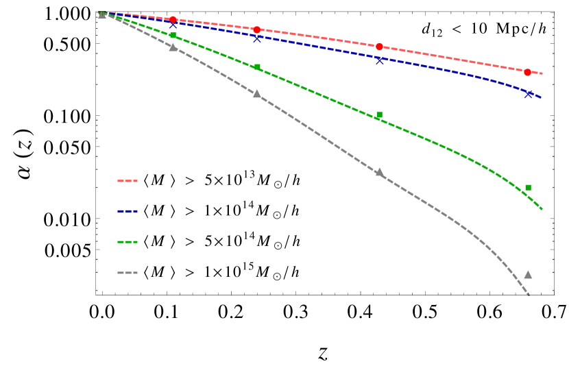
(a) The normalisation $\alpha(z)$ from Eq.(4.3) for various mass cuts, compared to simulation ‘data’.

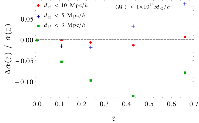
(b) The fractional difference in $\alpha(z)$ between the value extracted from the simulation and calculated using Eq.(4.3), for different separation cuts.

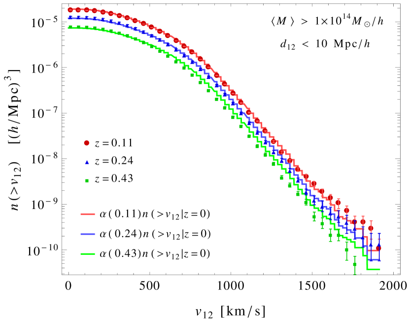
(c) Simulated ‘data’ on cumulative pairwise velocity distribution at various redshifts, compared to the approximation (4.2). Errors shown are estimated by bootstrapping.

Figure 1: Testing our semi-analytic model (4.2–4.3) against the DEUSS-Lambda N-Body simulation.

From Eqs. (4.1-4.3) it then follows that the number of Bullet-like systems factorises as:

$$N(<z)\approx n(v_{12}>v_{\rm Bullet},\mathrm{cuts}\mid z=0)\times V_{\rm eff}(z),$$ (4.4)

where:

$$V_{\rm eff}(z)=\int_{0}^{z}\alpha(z^{\prime})4\pi D_{c}^{2}(z^{\prime})\,\mathrm{d}D_{\mathrm{c}}(z^{\prime}).$$ (4.5)

Therefore, the pairwise velocity distribution can be studied at $z=0$ in simulation outputs, provided we can estimate (either semi-analytically as in Eq.(4.3), or from a set of smaller N-Body simulations) the effective volume $V_{\rm eff}$. This simplification is valid in the observationally interesting redshift range $z<1$.

Given that $V_{\rm eff}$ is big enough (such that the clustering of objects of interest is negligible), we can treat $N(<z)$ as being Poisson distributed. Then the probability that we see at least one object up to redshift $z$ is just: ${\rm Pr}\{N\geq 1\}=1-{\rm Poisson}\{N=0\mid\langle N\rangle=N(<z)\}$.

5 Results

Now we study the high-velocity tail of the pairwise velocity distribution, in particular its dependence on the collisional parameters — the average mass, the relative distance, the collisional angle, and the relative velocity of the halo pairs — and the correlations among these. The relative velocity of halo pairs, $v_{12}$, is considered in proper coordinates, i.e. including the Hubble flow term $\mathbf{v}_{\rm H}=H\mathbf{d}_{12}$. Using Eq.(4.2) we analyse the output of the N-Body simulation (Sec. 2) at redshift $z=0$.

Increasing the cut in the average mass $\langle M\rangle$ of the halo pairs, while keeping other collisional parameters (in particular $v_{12}$) unchanged, the number density of the halo pairs decreases as seen in Fig. 2. By contrast, if we chose to normalise the velocity distribution for each mass cut (as is done in Refs.[11, 14, 13, 10, 12]), we would conclude that the ‘probability’, i.e. the fraction of the high-velocity collisions, increases (see Fig. 3).

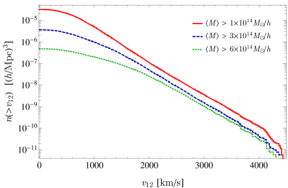
Figure 2: The dependence of the cumulative pairwise velocity distribution on the average mass $\langle M\rangle$ of the halo pairs. The halo mass function is steeply descending with $\langle M\rangle$, and so is the total number density of halo pairs, $n(>v_{12}=0|\langle M\rangle)$.

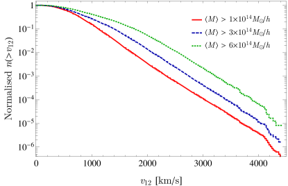
Figure 3: The cumulative pairwise velocity distribution normalised separately for each cut in the average mass. In the set of more massive halos, the fraction of higher relative velocity pairs is bigger. Naïvely this would be interpreted as a higher probability, however Fig. 2 shows that the absolute number density of more massive halos pairs decreases with $\langle M\rangle$.

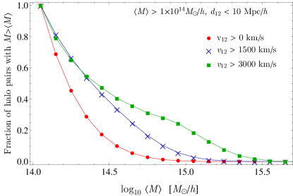
Figure 4: The fraction of halo pairs above a specified average mass $\langle M\rangle$, given the relative velocity $v_{12}$. The fraction of high-mass halo pairs is higher in the high-velocity population. Here $\langle M\rangle>10^{14}M_{\odot}/h$ and $d_{12}<10$ Mpc/h.

In Newtonian gravity, for a bound system with mass $m$ we expect $v_{12}\propto\sqrt{m}$. Therefore more massive halo pairs are likely to have a higher relative velocity. Indeed in Fig. 2 the tail of the low-$\langle M\rangle$ velocity distribution converges to the high-$\langle M\rangle$ tail at large relative velocities, indicating that the tail of the pairwise velocity distribution consists mostly of very massive halos. This is also seen in the mass distribution of halo pairs in the high-velocity tail (see Fig. 4). Therefore, small N-Body simulations that fail to produce halos with high masses underestimate the tail of the pairwise velocity distribution.

The next collisional parameter we examine is the angle $\theta$ between the separation and the relative velocity of a halo pair. In Fig. 5 we see that the tail of the velocity distribution consists almost entirely of the halo pairs approaching each other ($\cos\theta<0$). However, the number density of colliding halo pairs is not as sensitive to cuts in the angle as to the cuts in the halo masses. Again, as expected from Newtonian gravity, halo collisions with high relative velocity are more likely to be approximately head-on, as seen in Fig. 6.

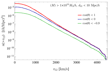
Figure 5: Cumulative pairwise velocity distribution for different cuts on the collisional angle $\theta$, taking $\langle M\rangle>10^{14}M_{\odot}/h$ and $d_{12}<10$ Mpc/h. Note that the high-velocity tail consists almost entirely of halos moving towards each other ($\cos\theta<0$).

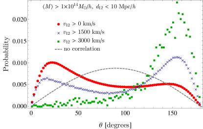
Figure 6: The probability distribution for the collisional angle $\theta$ given the relative velocity $v_{12}$, taking $\langle M\rangle>10^{14}M_{\odot}/h$ and $d_{12}<10$ Mpc/h. Small relative velocities are mainly associated with the Hubble flow, $\theta\sim 0^{\circ}$, whereas high velocities are mainly head-on collisions, $\theta\simeq 180^{\circ}$. The dashed line shows the case when the separation vector and the relative velocity vector are uncorrelated.

In Fig. 7 we see that the halo pairs with a high relative velocity are more likely to be closer together compared to the low pairwise velocity. Therefore, a configuration-space based halo finder (e.g. FoF) will miss relatively more high velocity mergers compared to the low velocity ones, and hence bias the tail of the pairwise velocity distribution to be shorter. This characteristic of the halo finders has been explored in greater detail in Ref.[14].

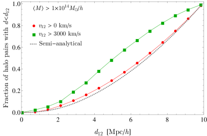
Figure 7: The fraction of halo pairs below a specified separation, given some relative velocity. For high-velocity collisions the halos are closer than for low pairwise velocities. The dashed line is the semi-analytical expectation for $v_{12}>0$ km/s, calculated using Eq.(4.3) with the cosmological parameters matching the Dark Sky simulation.

We have shown above that the number of Bullet-like systems has a non-trivial dependence on the collisional parameters, which are moreover correlated with each other. Therefore, the expected number of Bullet-like systems depends strongly on the adopted definition of such a system. A conservative (i.e. over-) estimate of the number of Bullet-like systems within a cosmic volume up to some redshift can be obtained by choosing cuts in the collisional parameters that are less extreme than those characterising 1E 0657-56. Accordingly, we adopt the following conditions on the average mass, separation, and the relative velocity of the halo pairs: $\langle M\rangle>10^{14}M_{\odot}/h,\text{ }d_{12}\leq 10\,\text{Mpc/h},\text{and }v_{12}>3000\,\text{km/s}$. This is comparable to the cuts made in Refs.[13] and [10]. Any additional cuts in the separation and the angle reduce the number of Bullet-like objects, thus exacerbating any tension of $\Lambda$CDM with observations. The pairwise velocity distribution and its cumulative version are shown in Figs. 8 and 9, where the errorbars have been estimated by a bootstrap technique. We fit the tail to the GPD form using the maximum likelihood method. The stability analysis is presented in Fig. 10. The appropriate choice for the threshold $\mu$ is around 1900 km/s; below this the events in the distribution are normal while above this threshold the variance increases substantially and the bias due to the finite simulation box appears (i.e. very rare events are missing altogether). Therefore the tail of the pairwise velocity distribution is well characterised by: $\mu\simeq 1900$ km/s, $\xi=0.038\pm 0.003$ and $\sigma=268.0\pm 1.4$ km/s. This is broadly consistent with the results of Ref.[13]. Thus the extreme events in the tail of the pairwise velocity distribution are not drawn from a Gaussian-like distribution ($\xi=0$) as has been assumed previously [12, 10, 14].

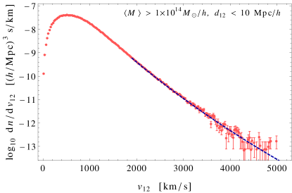
Figure 8: Pairwise velocity distribution from the simulation at redshift $z=0$ compared to the best fit Generalised Pareto Distribution.

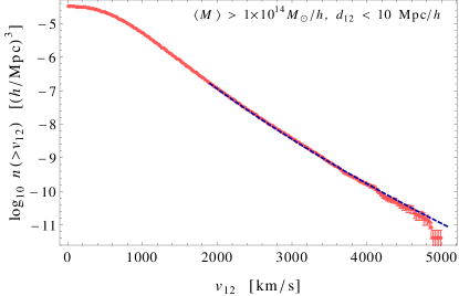
Figure 9: Cumulative pairwise velocity distribution from the simulation at redshift $z=0$ compared to the best fit Generalised Pareto Distribution.

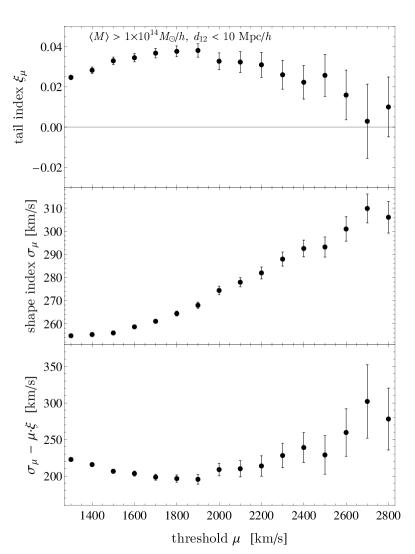
Figure 10: Stability plots for the EVS tail fitting exercise. The most appropriate threshold $\mu$ is seen to be around 1900 km/s where $\xi_{\mu}$ is approximately constant and $\sigma_{\mu}$ increases linearly.

We calculate the expected number of Bullet-like systems as defined above ($\langle M\rangle>10^{14}M_{\odot}/h,d_{12}\leq 10\,\text{Mpc}/h,\text{and }v_{12}>3000\,\text{km/s}$) up to $z=0.3$ (where 1E 0657-56 is located) and $z=0.5$ (where the initial conditions for the collision are known). The corresponding effective volumes from Eq. (4.5) are $V_{\rm eff}(<z=0.3)\simeq 4.6$ (Gpc/$h)^{3}$ and $V_{\rm eff}(<z=0.5)\simeq 13$ (Gpc/$h)^{3}$. Using this and the cumulative pairwise velocity distribution, the expected number of Bullet-like systems is:

$$N(<z=0.3)\simeq 17^{+6}_{-5},\text{ and }N(<z=0.5)\simeq 47^{+8}_{-7},$$ (5.1)

where the variance has been estimated by sampling the subvolumes of size $V_{\rm eff}$ from the full N-Body simulation.

We now focus on the expected number of objects as or more extreme than 1E 0657-56 in particular. Making cuts in the collisional parameters similar to Ref.[14]:

$$\langle M\rangle>(M_{\rm main}+M_{\rm Bullet})/2 =5.67\times 10^{14}M_{\odot}/h,\quad M_{1,2}>10^{14}M_{\odot}/h,$$

$$d_{12} \leq 10\,\text{Mpc}/h,\quad v_{12}>3000\,\text{km/s,}$$ (5.2)

we obtain:

$$N(<z=0.3)\simeq 1.3^{+2.0}_{-0.6}\quad\text{ and }\quad N(<z=0.5)\simeq 2.5^{+2.1}_{-1.2},$$ (5.3)

However since 1E 0657-56 is observed shortly after the collision we should require further that the halo pairs must be moving away from each other, i.e. $\cos\theta>0$. This leads to:

$$N(<z=0.3)\simeq 0.1\quad\text{ and }\quad N(<z=0.5)\simeq 0.15$$ (5.4)

Since the pairwise velocity distribution is steeply descending, increasing the relative velocity $v_{12}$ up to the 4500 km/s velocity of the shock front in the 1E 0657-56 merger would decrease this number further by two orders of magnitude, as we see from Fig. 2.

About a dozen other merging clusters have been observed, each with a different set of collisional parameters. Since a cluster collision is expected to take a short time compared to the cosmic time we can consider events both before and after collision by setting $\cos\theta<-0.9$ or $\cos\theta>0.9$. Requiring $v_{12}\geq 4000$ km/s in addition to the mass cuts in Eq.(5.2), we find only 4 halo pairs in the full (Hubble) volume of the simulation (see Table 1).

$M_{1}\left[M_{\odot}/h\right]$	$M_{2}\left[M_{\odot}/h\right]$	$d_{12}\left[\text{Mpc/h}\right]$	$v_{12}\left[\text{km/s}\right]$	$\cos\theta$
$1.73\times 10^{15}$	$1.1\times 10^{14}$	$6.9$	$4262$	$-0.99$
$3.11\times 10^{15}$	$1.2\times 10^{14}$	$8.3$	$4140$	$-0.96$
$3.0\times 10^{15}$	$1.3\times 10^{14}$	$2.7$	$4121$	$-0.93$
$3.8\times 10^{15}$	$1.4\times 10^{14}$	$3.5$	$4132$	$-0.94$

Table 1: Colliding halo pairs with the mass cuts from Eq.(5.2) and $v_{12}>4000$ km/s in the (8 Gpc/$h)^{3}$ Dark Sky simulation. All collisions are selected to be head-on ($|\cos\theta|>0.9$).

Hence, the expected number of such systems is $\langle N\rangle(<z=0.3)\simeq 0.02$, leading to the probability, $p(N\geq 1)=1-{\rm Poisson}(N=0\mid\langle N\rangle=0.02)\simeq 0.02$, of having at least one such system in a cosmic volume up to redshift $z=0.3$. Furthermore, setting $v_{12}\geq 4500$ km/s we find no candidate halo pairs. This places an upper limit of 0.005 on the probability $p(N\geq 1)$ of having at least one system with such an extreme relative velocity up to $z=0.3$.

For observers, an approximate formula for the number of colliding clusters expected up to a specified redshift, given specific collisional parameters, might be of interest:

$$N(<z;~{}<d_{12};~{}>v_{12};~{}>\langle M\rangle;~{}>\cos\theta)\approx A\langle M\rangle^{a}d_{12}^{b}z^{c}(1-\cos\theta)^{d}\times$$

$$\exp\left[\alpha\times(d_{12}/\langle M\rangle)+\cos^{2}\theta(\beta+\gamma\times\langle M\rangle+\delta\times v_{12})+v_{12}(\epsilon+\zeta\times d_{12})+\eta\times\langle M\rangle z\right],$$ (5.5)

where $(A,a,b,c,d,\alpha,\beta,\gamma,\delta,\epsilon,\zeta,\eta)=(80.7\times 10^{3},0.26,0.93,2.78,1.44,0.22,1.15,-0.071,2.50\times 10^{-4},-3.43\times 10^{-3},-4.82\times 10^{-5},-0.58)$. Our fit is valid to within 10% for $10^{14}M_{\odot}/h\lesssim\langle M\rangle\lesssim 7\times 10^{14}M_{\odot}/h$, $z<0.6$, $3\mathrm{\,Mpc/}h\lesssim d_{12}\lesssim 10\mathrm{\,Mpc/}h$, $\cos\theta\lesssim 0.9$, and $2000\mathrm{\,km/s}\lesssim v_{12}\lesssim 4000\mathrm{\,km/s}$. However it becomes unreliable at higher velocities and masses, as well as at lower separations. The effective volumes (4.5) used in the expression (5.5) above are in fact estimated from a set of smaller simulations [23].

6 Conclusions

We have studied the prevalence of rare DM halo collisions in $\Lambda$CDM cosmology using the pairwise velocity distribution for halos extracted from a N-body simulation with volume comparable to the observable universe and the finest resolution to date. Our approach differs from previous studies that attempt to quantify the probability that a cluster and its subcluster, given some masses and separation, will have a relative velocity as high as 1E 0657-56. We find that such a definition of probability can lead to paradoxical conclusions, so instead we investigate the dependence of the expected number of Bullet-like systems on the collisional parameters, as well as the correlations among them. We demonstrate that the expected number of halo pairs is very sensitive to cuts in the parameters defining the mergers. Given recent observations of more merging clusters, we provide a formula for the expected number of halo-halo collisions with specified collisional parameters up to some redshift.

The tail of the pairwise velocity distribution for the colliding halos is modelled using Extreme Values Statistics to demonstrate that it is fatter than a Gaussian. Hence, the combination of a configuration-space based halo finder, the assumption of a Gaussian-like tail, small simulation boxes, and poor simulation resolutions, have resulted in underestimation of the number of high-velocity mergers in previous studies.

We find that only about 0.1 systems like the Bullet Cluster 1E 0657-56 (where the collision has occurred already) can be expected up to $z=0.3$. Increasing the relative velocity to 4500 km/s — the shock front velocity deduced from X-ray observations of 1E 0657-56 — no candidate systems are found in the simulation. Thus the existence of 1E 0657-56 is only marginally compatible with the $\Lambda$CDM cosmology, provided the relative velocity of the two colliding clusters is indeed as low as suggested by hydrodynamical simulations. Hence if more such systems are found this would challenge the standard cosmological model.

7 Acknowledgements

DK thanks STFC for support and SS acknowledges a DNRF Niels Bohr Professorship. We are grateful to the anonymous Referee for emphasising the importance of the fact that the two clusters in 1E 0657-56 have collided already, and for several other helpful suggestions.

References

- [1] D. Clowe, A. Gonzalez, and M. Markevitch, Weak-Lensing Mass Reconstruction of the Interacting Cluster 1E 0657-558: Direct Evidence for the Existence of Dark Matter, Astrophys. J. 604 (Apr., 2004) 596–603, [astro-ph/0312273].
- [2] M. Bradač, D. Clowe, A. H. Gonzalez, P. Marshall, W. Forman, C. Jones, M. Markevitch, S. Randall, T. Schrabback, and D. Zaritsky, Strong and Weak Lensing United. III. Measuring the Mass Distribution of the Merging Galaxy Cluster 1ES 0657-558, Astrophys. J. 652 (Dec., 2006) 937–947, [astro-ph/0608408].
- [3] M. Markevitch, A. H. Gonzalez, D. Clowe, A. Vikhlinin, W. Forman, C. Jones, S. Murray, and W. Tucker, Direct Constraints on the Dark Matter Self-Interaction Cross Section from the Merging Galaxy Cluster 1E 0657-56, Astrophys. J. 606 (May, 2004) 819–824, [astro-ph/0309303].
- [4] G. R. Farrar and R. A. Rosen, A New Force in the Dark Sector?, Phys. Rev. Lett. 98 (Apr., 2007) 171302, [astro-ph/0610298].
- [5] C. Lage and G. Farrar, Constrained Simulation of the Bullet Cluster, Astrophys. J. 787 (June, 2014) 144, [arXiv:1312.0959].
- [6] C. Lage and G. R. Farrar, The Bullet Cluster is not a Cosmological Anomaly, ArXiv e-prints (June, 2014) [arXiv:1406.6703].
- [7] C. Mastropietro and A. Burkert, Simulating the Bullet Cluster, Mon. Not. R. Astron. Soc. 389 (Sept., 2008) 967–988, [arXiv:0711.0967].
- [8] V. Springel and G. R. Farrar, The speed of the ‘bullet’ in the merging galaxy cluster 1E0657-56, Mon. Not. R. Astron. Soc. 380 (Sept., 2007) 911–925, [astro-ph/0703232].
- [9] M. Milosavljević, J. Koda, D. Nagai, E. Nakar, and P. R. Shapiro, The Cluster-Merger Shock in 1E 0657-56: Faster than a Speeding Bullet?, Astron. J. Lett. 661 (June, 2007) L131–L134, [astro-ph/0703199].
- [10] R. Thompson and K. Nagamine, Pairwise velocities of dark matter haloes: a test for the cold dark matter model using the bullet cluster, Mon. Not. R. Astron. Soc. 419 (Feb., 2012) 3560–3570, [arXiv:1107.4645].
- [11] E. Hayashi and S. D. M. White, How rare is the bullet cluster?, Mon. Not. R. Astron. Soc. 370 (July, 2006) L38–L41, [astro-ph/0604443].
- [12] J. Lee and E. Komatsu, Bullet Cluster: A Challenge to CDM Cosmology, Astrophys. J. 718 (July, 2010) 60–65, [arXiv:1003.0939].
- [13] V. R. Bouillot, J.-M. Alimi, P.-S. Corasaniti, and Y. Rasera, Probing dark energy models with extreme pairwise velocities of galaxy clusters from the DEUS-FUR simulations, ArXiv e-prints (May, 2014) [arXiv:1405.6679].
- [14] R. Thompson, R. Davé, and K. Nagamine, The rise and fall of a challenger: the Bullet Cluster in Cold Dark Matter simulations, ArXiv e-prints (Oct., 2014) [arXiv:1410.7438].
- [15] P. S. Behroozi, R. H. Wechsler, and H.-Y. Wu, The ROCKSTAR Phase-space Temporal Halo Finder and the Velocity Offsets of Cluster Cores, Astrophys. J. 762 (Jan., 2013) 109, [arXiv:1110.4372].
- [16] W. A. Watson, I. T. Iliev, J. M. Diego, S. Gottlöber, A. Knebe, E. Martínez-González, and G. Yepes, Statistics of extreme objects in the Juropa Hubble Volume simulation, Mon. Not. R. Astron. Soc. 437 (Feb., 2014) 3776–3786, [arXiv:1305.1976].
- [17] J. E. Forero-Romero, S. Gottlöber, and G. Yepes, Bullet Clusters in the MARENOSTRUM Universe, Astrophys. J. 725 (Dec., 2010) 598–604, [arXiv:1007.3902].
- [18] J. Lee and M. Baldi, Can Coupled Dark Energy Speed up the Bullet Cluster?, Astrophys. J. 747 (Mar., 2012) 45, [arXiv:1110.0015].
- [19] S. W. Skillman, M. S. Warren, M. J. Turk, R. H. Wechsler, D. E. Holz, and P. M. Sutter, Dark Sky Simulations: Early Data Release, ArXiv e-prints (July, 2014) [arXiv:1407.2600].
- [20] J. F. Navarro, C. S. Frenk, and S. D. M. White, The Structure of Cold Dark Matter Halos, Astrophys. J. 462 (May, 1996) 563, [astro-ph/9508025].
- [21] L. Hernquist, N-body realizations of compound galaxies, Astrophys. J. Suppl. 86 (June, 1993) 389–400.
- [22] S. Coles, An Introduction to Statistical Modeling of Extreme Values. Lecture Notes in Control and Information Sciences. Springer, 2001.
- [23] Y. Rasera, J.-M. Alimi, J. Courtin, F. Roy, P.-S. Corasaniti, A. Füzfa, and V. Boucher, Introducing the dark energy universe simulation series (DEUSS), vol. 1241, pp. 1134–1139, June, 2010. arXiv:1002.4950.
- [24] J. L. Tinker, B. E. Robertson, A. V. Kravtsov, A. Klypin, M. S. Warren, G. Yepes, and S. Gottlöber, The Large-scale Bias of Dark Matter Halos: Numerical Calibration and Model Tests, Astrophys. J. 724 (Dec., 2010) 878–886, [arXiv:1001.3162].
- [25] J. L. Tinker, D. H. Weinberg, Z. Zheng, and I. Zehavi, On the Mass-to-Light Ratio of Large-Scale Structure, Astrophys. J. 631 (Sept., 2005) 41–58, [astro-ph/0411777].