Greedy Algorithms for Steiner Forest

Abstract

In the Steiner Forest problem, we are given terminal pairs $\{s_{i},t_{i}\}$, and need to find the cheapest subgraph which connects each of the terminal pairs together. In 1991, Agrawal, Klein, and Ravi, and Goemans and Williamson gave primal-dual constant-factor approximation algorithms for this problem; until now the only constant-factor approximations we know are via linear programming relaxations.

In this paper, we consider the following greedy algorithm:

Given terminal pairs in a metric space, a terminal is active if its distance to its partner is non-zero. Pick the two closest active terminals (say $s_{i},t_{j}$), set the distance between them to zero, and buy a path connecting them. Recompute the metric, and repeat.

It has long been open to analyze this greedy algorithm. Our main result: this algorithm is a constant-factor approximation.

We use this algorithm to give new, simpler constructions of cost-sharing schemes for Steiner forest. In particular, the first “strict” cost-shares for this problem implies a very simple combinatorial sampling-based algorithm for stochastic Steiner forest.

1 Introduction

In the Steiner forest problem, given a metric space and a set of source-sink pairs $\{s_{i},t_{i}\}_{i=1}^{K}$, a feasible solution is a forest such that each source-sink pair lies in the same tree in this forest. The goal is to minimize the cost, i.e., the total length of edges in the forest. This problem is a generalization of the Steiner tree problem, and hence APX-hard. The constant-factor approximation algorithms currently known for it are all based on linear programming techniques. The first such result was an influential primal-dual $2$-approximation due to Agrawal, Klein, and Ravi [AKR95]; this was simplified by Goemans and Williamson [GW95] and extended to many “constrained forest” network design problems. Other works have since analyzed the integrality gaps of the natural linear program, and for some stronger LPs; see §​ 1.2.

However, no constant-factor approximations are known based on “purely combinatorial” techniques. Some natural algorithms have been proposed, but these have defied analysis for the most part. The simplest is the paired greedy algorithm that repeatedly connects the yet-unconnected $s_{i}$-$t_{i}$ pair at minimum mutual distance; this is no better than $\Omega(\log n)$ (see Chan, Roughgarden, and Valiant [CRV10] or Appendix A). Even greedier is the so-called gluttonous algorithm that connects the closest two yet-unsatisfied terminals regardless of whether they were “mates”. The performance of this algorithm has been a long-standing open question. Our main result settles this question.

Theorem 1.1

The gluttonous algorithm is a constant-factor approximation for Steiner Forest.

We then apply this result to obtain a simple combinatorial approximation algorithm for the two-stage stochastic version of the Steiner forest problem. In this problem, we are given a probability distribution $\pi$ defined over subsets of demands. In the first stage, we can buy some set $E_{1}$ of edges. Then in the second stage, the demand set is revealed (drawn from $\pi$), and we can extend the set $E_{1}$ to a feasible solution for this demand set. However, these edges now cost $\sigma>1$ times more than in the first stage. The goal is to minimize the total expected cost. It suffices to specify the set $E_{1}$—once the actual demands are known, we can augment using our favorite approximation algorithm for Steiner forest. Our simple algorithm is the following: sample $\lceil\sigma\rceil$ times from the distribution $\pi$, and let $E_{1}$ be the Steiner forest constructed by (a slight variant of) the gluttonous algorithm on union of these $\lceil\sigma\rceil$ demand sets sampled from $\pi$.

Theorem 1.2

There is a combinatorial (greedy) constant-factor approximation algorithm for the stochastic Steiner forest problem.

Showing that such a “boosted sampling” algorithm obtained a constant factor approximation had proved elusive for several years now; the only constant-factor approximation for stochastic Steiner forest was a complicated primal-dual algorithm with a worse approximation factor [GK09]. Our result is based on the first cost sharing scheme for the Steiner forest problem which is constant strict with respect to a constant factor approximation algorithm; see §​ 5 for the formal definition. Such a cost sharing scheme can be used for designing approximation algorithms for several stochastic network design problems for the Steiner forest problem. In particular, we obtain the following results:

• For multi-stage stochastic optimization problem for Steiner forest, our strict-cost sharing scheme along with the fact that it is also cross-monotone implies the first $O(1)^{k}$-approximation algorithm, where $k$ denotes the number of stages (see [GPRS11] for formal definitions and the relation with cost sharing).

• Consider the online stochastic problem, where given a set of source-sink pairs ${\mathscr{D}}$ in a metric ${\mathcal{M}}$, and a probability distribution $\pi$ over subsets of ${\mathscr{D}}$ (i.e., over $2^{{\mathscr{D}}}$), an adversary chooses a parameter $k$, and draws $k$ times independently from $\pi$. The on-line algorithm, which can sample from $\pi$, needs to maintain a feasible solution over the set of demand pairs produced by the adversary at all time. The goal is to minimize the expected cost of the solution produced by the algorithm, where the expectation is over $\pi$ and random coin tosses of the algorithm. Our cost sharing framework gives the first constant competitive algorithm for this problem, generalizing the result of Garg et al. [GGLS08] which works for the special case when $\pi$ is a distribution over ${\mathscr{D}}$ (i.e., singleton subsets of ${\mathscr{D}}$).

1.1 Ideas and Techniques

We first describe the gluttonous algorithm. Call a terminal active if it is not yet connected to its mate. Recall: our algorithm merges the two active terminals that are closest in the current metric (and hence zeroes out their distance). At any point of time, we have a collection of supernodes, each supernode corresponding to the set of terminals which have been merged together. A supernode is active if it contains at least one active terminal. Hence the algorithm can be alternatively described thus: merge the two active supernodes that are closest (in the current metric) into a new supernode. (A formal description of the algorithm appears in §2.)

The analysis has two conceptual steps. In the first step, we reduce the problem to the special case when the optimal solution can be (morally) assumed to be a single tree (formally, we reduce to the case where the gluttonous’ solution is a refinement of the optimal solution). The proof for this part is simple: we take an optimal forest, and show that we can connect two trees in the forest if the gluttonous algorithm connects two terminals lying in these two trees, incurring only a factor-of-two loss.

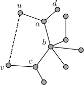
Figure 1.1: Example showing the construction of tree $T^{\prime}$ from $T$, which is shown in solid lines. If we merge $u$ and $u^{\prime}$, we can remove the edge $(a,b)$ to get the tree $T^{\prime}$. Assuming $a$ is not active, we can also short-cut the degree 2 vertex $a$ in $T^{\prime}$ by replacing the edges $(s,a)$ and $(a,d)$ with the edge $(s,d)$.

The second step of the analysis starts with the tree solution $T$ promised by the first step of the analysis. As the gluttonous algorithm proceeds, the analysis alters $T$ to maintain a candidate solution to the current set of supernodes. E.g., if we merge two active supernodes $u$ and $v$ to get a new supernode $uv$. We want to alter the solution $T$ on the original supernodes to get a new solution $T^{\prime}$, say by removing an edge from the (unique) $u$-$v$ path in $T$, and then short-cutting any degree two inactive supernode in $T^{\prime}$ (see Figure 1.1 for an example). The hope is to argue that the distance between $u$ and $v$—which is the cost incurred by gluttonous—is commensurate to the cost of the edge of $T$ which gets removed during this process. This would be easy if there were a long edge on $u$-$v$ path in the tree $T$. The problem: this may not hold for every pair of supernodes we merge. Despite this, our analysis shows that the bad cases cannot happen too often, and so we can perform this charging argument in an amortized sense.

Our analysis is flexible and extends to other variants of the gluttonous algorithm. A natural variant is one where, instead of merging the two closest active supernodes, we contract the edges on a shortest path between the two closest active supernodes. The first step of the above analysis does not hold any more. However, we show that it is enough to account for the merging cost of supernodes when the active terminals in them lie in the same tree of the optimal solution, and consequently the arguments in the second step of the analysis are sufficient. Yet another variant is a timed version of the algorithm, which is inspired by a timed version of the primal-dual algorithm [KLSvZ08], and is crucial for obtaining the strict cost-shares described next.

Loosely speaking, a cost-sharing method takes an algorithm ${\mathscr{A}}$ and divides the cost incurred by the algorithm on an instance among the terminals ${\mathscr{D}}$ in that instance. The “strictness” property ensures that if we partition ${\mathscr{D}}$ arbitrarily into ${\mathscr{D}}_{1}\cup{\mathscr{D}}_{2}$, and build a solution ${\mathscr{A}}({\mathscr{D}}_{1})$ on ${\mathscr{D}}_{1}$, then the cost-shares of the terminals in ${\mathscr{D}}_{2}$ would suffice to augment the solution ${\mathscr{A}}({\mathscr{D}}_{1})$ to one for ${\mathscr{D}}_{2}$ as well.

A natural candidate for ${\mathscr{A}}$ is the GW primal-dual algorithm, and the cost-shares are equally natural: we divide up the cost of growing moats among the active terminals in the moat. However, the example in Figure 1.2 shows why this fails when ${\mathscr{D}}_{2}$ consists of just the demand pair $\{s,\bar{s}\}$. When run on all the terminals, the primal-dual algorithm stops at time 1, with all terminals getting a cost-share of 1. On the other hand, if we run ${\mathscr{A}}$ on ${\mathscr{D}}_{1}$, it finds a solution which has $N$ connected components, each connecting $s_{i}$ and ${\bar{s}}_{i}$ for $i=1,\ldots,N$. Then connecting $s$ and $\bar{s}$ costs $2N$, which is much more than their total cost share.

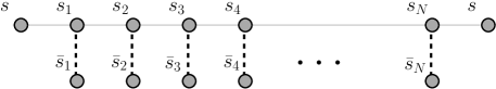
Figure 1.2: Distances $d(s_{i},{\bar{s}}_{i})$ are 2 for all $i$. Further, $d(s_{i},s_{i+1})=d({\bar{s}}_{i},{\bar{s}}_{i+1})=2$ for $i=1,\ldots,N-1$. The distances $d(s,s_{1})$ and $d(s_{N},{\bar{s}})$ are slightly larger than 2. The dotted lines indicate the forest returned by the GW primal-dual algorithm when run on the demand set $\{(s_{i},{\bar{s}}_{i}):i=1,\ldots,N\}$

To avoid this problem, [GKPR07, FKLS10] run the primal-dual algorithm for longer than required, and give results for the case when ${\mathscr{D}}_{2}$ contains a single demand pair. However, the arguments become much more involved than those in the analysis of GW algorithm [GW95]—the main reason is the presence of “dead” moats which cause some edges to become tight, and the cost shares of active terminals cannot account for such edges. In our case, the combinatorial (greedy) nature of our algorithm/analysis means we do not face such issues. As a result, we can obtain such strict cost sharing methods (when ${\mathscr{D}}_{2}$ is a singleton set) with much simpler analysis, albeit with worse constants than those in [GKPR07, FKLS10]). We refer to this special case of strictness property as uni-strictness.

Our analysis for the general case where ${\mathscr{D}}_{2}$ contains multiple demand pairs requires considerably more work; but note that these are the first known strict cost shares for this case, the previous primal-dual techniques could not handle the complexity of this general case. Here, we want ${\mathscr{A}}$ to build as many edges as possible, and the cost share $\chi$ to be as large as possible. Since the gluttonous algorithm tends to build fewer edges than primal-dual (the dead moats causing extra connections and more edges), we end up using the primal-dual algorithm as the algorithm ${\mathscr{A}}$. However, to define the cost-shares, we use the (timed) gluttonous algorithm in order to avoid the issues with dead moats. The analysis then proceeds via showing a close correspondence between the primal-dual and gluttonous algorithms. Although this is not involved, it needs to carefully match the two runs.

1.1.1 Outline of Paper

We first describe some related work in §​ 1.2, and give some important definitions in §​ 1.3. Then we describe the gluttonous algorithm formally in §​ 2, and then analyze this algorithm in §​ 3. We then show that our analysis is flexible enough to analyze several variants of the gluttonous algorithm. We study the the timed version in §​ 4, which gets used in subsequent sections on cost sharing. We also consider the variant of gluttonous based on path-contraction in the appendix (see Appendix B). The cost-sharing method for the uni-strict case is in §​ 5, and the general case is in §​ 5.2.

1.2 Related Work

The first constant-factor approximation algorithm for the Steiner forest problem was due to Agrawal, Klein, and Ravi [AKR95] using a primal-dual approach; it was refined and generalized by Goemans and Williamson [GW95] to a wider class of network design problems. The primal-dual analysis also bounds integrality gap of the the natural LP relaxation (based on covering cuts) by a factor of $2$. Different approximation algorithms for Steiner forest based off the same LP, and achieving the same factor of $2$, are obtained using the iterative rounding technique of Jain [Jai01], or the integer decomposition techniques of Chekuri and Shepherd [CS09]. A stronger LP relaxation was proposed by Könemann, Leonardi, and Schäfer [KLS05], but it also has an integrality gap of $2$ [KLSvZ08].

The special case of the Steiner tree problem, where all the demands share a common (source) terminal, has been well-studied in the network design community. There is a simple 2-approximation algorithm for this problem: iteratively find the closest terminal to the source vertex, and merge these two terminals. There have been several changes to this simple greedy algorithm leading to improved approximation ratios (see e.g. [RZ05]). Byrka et al. [BGRS13] improved these results to a $\ln 4+\varepsilon\approx 1.46$-approximation algorithm, which is based on rounding a stronger LP relaxation for this problem.

The stochastic Steiner tree/forest problem was defined by Immorlica, Karger, Minkoff, and Mirrokni [IKMM04], and further studied by [GPRS11], who proposed the boosted-sampling framework of algorithms. The analysis of these algorithms is via “strict” cost sharing methods, which were studied by [GKPR07, FKLS10]. A constant-factor approximation algorithm (with a large constant) was given for stochastic Steiner forest by [GK09] based on primal-dual techniques; it is much more complicated than the algorithm and analysis based on the greedy techniques in this paper.

1.3 Preliminaries

Let ${\mathcal{M}}=(V,d)$ be a metric space on $n$ points; assume all distances are either $0$ or at least $1$. Let the demands ${\mathscr{D}}\subseteq\binom{V}{2}$ be a collection of source-sink pairs that need to be connected. By splitting vertices, we may assume that the pairs in ${\mathscr{D}}$ are disjoint. A node is a terminal if it belongs to some pair in ${\mathscr{D}}$. Let $K$ denote the number of terminals pairs, and hence there are $2K$ terminals. For a terminal $u$, let $\bar{u}$ be the unique vertex such that $\{u,\bar{u}\}\in{\mathscr{D}}$; we call $\bar{u}$ the mate of $u$.

For a Steiner forest instance ${\mathscr{I}}=({\mathcal{M}},{\mathscr{D}})$, a solution ${\mathscr{F}}$ to the instance ${\mathscr{I}}$ is a forest such that each pair $\{u,\bar{u}\}\in{\mathscr{D}}$ is contained within the vertex set $V(T)$ for some tree $T\in{\mathscr{F}}$. For a tree $T=(V,E_{T})$, let $\mathsf{cost}(T):=\sum_{e\in E_{T}}d(e)$ be the sum of lengths of edges in $T$. Let $\mathsf{cost}({\mathscr{F}}):=\sum_{T\in{\mathscr{F}}}\mathsf{cost}(T)$ be the cost of the forest ${\mathscr{F}}$. Our goal is to find a solution of minimum cost.

2 The Gluttonous Algorithm

To describe the gluttonous algorithm, we need some definitions. Given a Steiner forest instance ${\mathscr{I}}=({\mathcal{M}},{\mathscr{D}})$, a supernode is a subset of terminals. A clustering ${\mathscr{C}}=\{S_{1},S_{2},\ldots,S_{q}\}$ is a partition of the terminal set into supernodes. The trivial clustering places each terminal in its own singleton supernode. Our algorithm maintains a clustering at all points in time. Given a clustering, a terminal $u$ is active if it belongs to a supernode $S$ that does not contain its mate $\bar{u}$. A supernode $S$ is active if it contains some active terminal. In the trivial clustering, all the terminals and supernodes are active.

Given a clustering ${\mathscr{C}}=(S_{1},S_{2},\ldots,S_{q})$, define a new metric ${\mathcal{M}}/{\mathscr{C}}$ called the ${\mathscr{C}}$-puncturing of metric ${\mathcal{M}}$. To get this, take a complete graph on $V$; for an edge $\{u,v\}$, set its length to be $d(u,v)$ if $u,v$ lie in different supernodes in ${\mathscr{C}}$, and to zero if $u,v$ lie in the same supernode in ${\mathscr{C}}$. Call this graph $G_{\mathscr{C}}$, and defined the ${\mathscr{C}}$-punctured distance to be the shortest-path distance in this graph, denoted by $d_{{\mathcal{M}}/{\mathscr{C}}}(\cdot,\cdot)$. One can think of this as modifying the metric ${\mathcal{M}}$ by collapsing the terminals in each of the supernodes in ${\mathscr{C}}$ to a single node. Given clustering ${\mathscr{C}}$ and two supernodes $S_{1}$ and $S_{2}$, the distance between them is naturally defined as

$$d_{{\mathcal{M}}/{\mathscr{C}}}(S_{1},S_{2})=\min_{u\in S_{1},v\in S_{2}}d_{{\mathcal{M}}/{\mathscr{C}}}(u,v).$$

The gluttonous algorithm is as follows:

Start with ${\mathscr{C}}$ being the trivial clustering, and $E^{\prime}$ being the empty set. While there exist active supernodes in ${\mathscr{C}}$, do the following:

• Find active supernodes $S_{1},S_{2}$ in ${\mathscr{C}}$ with minimum ${\mathscr{C}}$-punctured distance. (Break ties arbitrarily but consistently, say choosing the lexicographically smallest pair.)

• Update the clustering to

  $${\mathscr{C}}\leftarrow({\mathscr{C}}\setminus\{S_{1},S_{2}\})\cup\{S_{1}\cup S_{2}\},$$

• Add to $E^{\prime}$ the edges corresponding to the inter-supernode edges on the shortest path between $S_{1},S_{2}$ in the graph $G_{\mathscr{C}}$.

Finally, output a maximal acyclic subgraph $F$ of $E^{\prime}$.

Above, we say we merge $S_{1},S_{2}$ to get the new supernode $S_{1}\cup S_{2}$. The merging distance for the merge of $S_{1},S_{2}$ is the ${\mathscr{C}}$-punctured distance $d_{{\mathcal{M}}/{\mathscr{C}}}(S_{1},S_{2})$, where ${\mathscr{C}}$ is the clustering just before the merge. Since each active supernode contains an active terminal, if $u\in S_{1}$ and $v\in S_{2}$ are both active, then when we talk about merging $u,v$, we mean merging $S_{1},S_{2}$.

Note that the length of the edges added in step (iii) is equal to $d_{{\mathcal{M}}/{\mathscr{C}}}(S_{1},S_{2})$. The algorithm maintains the following invariant: if $S$ is a supernode, then the terminals in $S$ lie in the same connected component of $F$. The algorithm terminates when there are no more active terminals, so each terminal shares a supernode with its mate, and hence the final forest $F$ connects all demand pairs. Since the edges added to $E^{\prime}$ have total length at most the sum of the merging distances, and we output a maximal sub-forest of $E^{\prime}$, we get:

Fact 2.1

The cost of the Steiner forest solution output is at most the sum of all the merging distances.

We emphasize that the edges added in Step (iii) are often overkill: the metric ${\mathcal{M}}/E^{\prime}$ (where the edges in $E^{\prime}$ have been contracted) has no greater distances than the metric ${\mathcal{M}}/{\mathscr{C}}$ that we focus on. The advantage of the latter over the former is that distances in ${\mathcal{M}}/{\mathscr{C}}$ are well-controlled (and distances between active terminals only increase over time), whereas those in ${\mathcal{M}}/E^{\prime}$ change drastically over time (with distances between active terminals changing unpredictably).

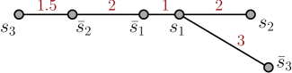
Figure 2.3: Figure for the gluttonous algorithm.

Consider the example in Figure 2.3, where the distances for missing edges are inferred by computing shortest-path distances.

Here, we first merge $\{s_{1},{\bar{s}}_{1}\}$ to form a supernode, say $A$, which is inactive. Next we merge $s_{3}$ and ${\bar{s}}_{2}$ to form another supernode, say $B$. The active supernodes are $B,s_{2}$, and $\bar{s}_{3}$, so we next merge $s_{2}$ with $B$ to form supernode $C$, and finally merge ${\bar{s}}_{3}$ with $C$. When the algorithm ends, there are two (inactive) supernodes corresponding to the sets $\{s_{1},{\bar{s}}_{1}\}$ and $\{s_{2},s_{3},{\bar{s}}_{2},{\bar{s}}_{3}\}$. However, the forest produced will have only a single tree, which consists of the set of edges drawn in the figure.

3 The Analysis for Gluttonous

We analyze the algorithm in two steps. One conceptual problem is in controlling what happens when gluttonous connects two nodes in different trees of the optimal forest. To handle this, we show in §​ 3.2 how to preprocess the optimal forest $\mathscr{F}^{\star}$ to get a near-optimal forest $\mathscr{F}^{\star\star}$ such that the final clustering of the gluttonous algorithm is a refinement of this near-optimal forest. (I.e., if $u$ and $v$ are in the same supernode in the gluttonous clustering, then they lie in the same tree in $\mathscr{F}^{\star\star}$.) This makes it easier to then account for the total merging distance, which we do in §​ 3.3.

3.1 Monotonicity Properties

To begin, some simple claims about monotonicity. The first one is by definition.

Fact 3.1 (Distance Functions are Monotone)

Let the clustering ${\mathscr{C}}^{\prime}$ correspond to a later time than the clustering ${\mathscr{C}}$. Then ${\mathscr{C}}$ is a refinement of ${\mathscr{C}}^{\prime}$. Moreover, $d_{{\mathcal{M}}/{\mathscr{C}}^{\prime}}(u,v)\leq d_{{\mathcal{M}}/{\mathscr{C}}}(u,v)$ for all $u,v\in V$.

Claim 3.2

Consider clustering ${\mathscr{C}}$ and let any two active supernodes $S,T$ be merged, resulting in clustering ${\mathscr{C}}^{\prime}$. Then for any active $U\in{\mathscr{C}}$ that is not $S$ or $T$, the distance to its closest active supernode does not decrease. Also, if $S\cup T$ is active in ${\mathscr{C}}^{\prime}$ then the distance to its closest supernode in ${\mathscr{C}}^{\prime}$ is at least as large as the minimum of $S$ and $T$’s distances to their closest supernodes in ${\mathscr{C}}$.

Proof.

First observe that when two active supernodes are merged, they may stay active or become inactive. An inactive supernode never merges with any other supernode, and hence, it cannot become active later.

For active supernode $U\neq S,T$, suppose its closest supernode in ${\mathscr{C}}$ was $W$ at ${\mathscr{C}}$-punctured distance $L$, and in ${\mathscr{C}}^{\prime}$ it is $W^{\prime}$ at ${\mathscr{C}}^{\prime}$-punctured distance $L^{\prime}$. If $L^{\prime}<L$, there must now be a path through supernode $S\cup T$ that is of length $L^{\prime}$. But this means the ${\mathscr{C}}$-punctured distance of $U$ from either $S$ or $T$ was at most $L^{\prime}$, and both were active in ${\mathscr{C}}$—a contradiction. This proves the first part of the claim.

Now, suppose supernode $U:=S\cup T$ is active in ${\mathscr{C}}^{\prime}$. Observe that for any other supernode $W\in{\mathscr{C}}^{\prime}$, the punctured distance $d_{{\mathcal{M}}/{\mathscr{C}}^{\prime}}(U,W)=\min\{d_{{\mathcal{M}}/{\mathscr{C}}}(S,W),d_{{\mathcal{M}}/{\mathscr{C}}}(T,W)\}$. This proves the second part of the claim. ∎

Claim 3.3 (Gluttonous Merging Distances are Monotone)

If $S,T$ are merged before $S^{\prime},T^{\prime}$ in gluttonous, then the merging distance for $S,T$ is no greater than the merging distance for $S^{\prime},T^{\prime}$.

Proof.

Gluttonous merges two active supernodes with the smallest current distance. By Claim 3.2 distances between the remaining active supernodes do not decrease. This proves this claim. ∎

3.2 A Near-Optimal Solution with Good Properties

Since gluttonous is deterministic and we break ties consistently, given an instance Steiner forest instance ${\mathscr{I}}=({\mathcal{M}},{\mathscr{D}})$ there is a unique final clustering ${\mathscr{C}}^{f}$ produced by the algorithm.

Definition 3.4 (Faithful)

A forest ${\mathscr{F}}$ is faithful to a clustering ${\mathscr{C}}$ if each supernode $S\in{\mathscr{C}}$ is contained within a single tree in ${\mathscr{F}}$. (I.e., for all $S\in{\mathscr{C}}$, there exists $T\in{\mathscr{F}}$ such that $S\subseteq V(T)$.)

Note that every forest is faithful to the trivial clustering consisting of singletons.

Definition 3.5 (Width)

For a forest ${\mathscr{F}}$ that is a solution to instance ${\mathscr{I}}$, and for any tree $T\in{\mathscr{F}}$, let $0pt(T)$ denote the largest tree distance between any pair connected by $T$. Let the width of forest ${\mathscr{F}}$ be the sum of the widths of the trees in ${\mathscr{F}}$. I.e.,

$$0pt(T) :=\max\{d_{T}(u,\bar{u})\mid\{u,\bar{u}\}\in{\mathscr{D}},\{u,\bar{u}\}\subseteq V(T)\},$$ (3.1)

$$0pt({\mathscr{F}}) :=\textstyle\sum_{T\in F}0pt(T),$$ (3.2)

where $d_{T}$ refers to the tree metric induced by $T$.

We now show there exist near-optimal solutions which are faithful to gluttonous’ final clustering.

Theorem 3.6 (Low-Cost and Faithful)

Let $\mathscr{F}^{\star}=\{T_{1}^{\star},T_{2}^{\star},\ldots,T_{p}^{\star}\}$ be an optimal solution to the Steiner forest instance ${\mathscr{I}}=({\mathcal{M}},{\mathscr{D}})$. There exists another solution $\mathscr{F}^{\star\star}$ for instance ${\mathscr{I}}$ such that

• $\mathsf{cost}(\mathscr{F}^{\star\star})\leq\mathsf{cost}(\mathscr{F}^{\star})+0pt(\mathscr{F}^{\star})\leq 2\mathsf{cost}(\mathscr{F}^{\star})$, and

• $\mathscr{F}^{\star\star}$ is faithful to the final clustering ${\mathscr{C}}^{f}$ produced by the gluttonous algorithm.

Proof.

Start with $\mathscr{F}^{\star\star}=\mathscr{F}^{\star}$ which clearly satisfies the first (cost) guarantee but perhaps not the second (faithfulness) one. To fix this, run the gluttonous algorithm on ${\mathscr{I}}$, and whenever it connects two terminals $(u,v)$ that violate the condition (b), connect up some trees in the current $\mathscr{F}^{\star\star}$ to prevent this violation. In particular, we show how to do this while maintaining two invariants:

• The cost of edges in $\mathscr{F}^{\star\star}\setminus\mathscr{F}^{\star}$ is at most $0pt(\mathscr{F}^{\star})-0pt(\mathscr{F}^{\star\star})$, and

• at any point in time, the forest $\mathscr{F}^{\star\star}$ is faithful to the current clustering ${\mathscr{C}}$ (during the run of the gluttonous algorithm).

At the beginning, the clustering ${\mathscr{C}}$ is the trivial clustering consisting of singleton sets containing terminals, and $\mathscr{F}^{\star\star}=\mathscr{F}^{\star}$; both invariants (A) and (B) are vacuously true.

Now consider some step of gluttonous which starts with the clustering ${\mathscr{C}}$ and connects two active supernodes $S$ and $S^{\prime}$ which are closest to each other to get the clustering ${\mathscr{C}}^{\prime}$. By the invariant (B), we know all terminals in supernode $S$ lie within the same tree in $\mathscr{F}^{\star\star}$, and the same for terminals in $S^{\prime}$. Let $u\in S$ and $v\in S^{\prime}$ be some active terminals within these supernodes; hence $\bar{u}\not\in S$ and $\bar{v}\not\in S^{\prime}$. Two cases arise:

• Case I: $u$ and $v$ belong to the same tree in $\mathscr{F}^{\star\star}$: Clearly, $\mathscr{F}^{\star\star}$ satisfies the invariant (B) with respect to ${\mathscr{C}}^{\prime}$ as well. Hence, we keep $\mathscr{F}^{\star\star}$ unchanged and it satisfies invariant (A) trivially.

• Case II: $u$ and $v$ belong to different trees $T_{1}^{\star\star},T_{2}^{\star\star}\in\mathscr{F}^{\star\star}$: Suppose the shortest path between $u$ and $v$ in ${\mathcal{M}}/{\mathscr{C}}$ is

  $$P=\{u=x_{0},x_{0}^{\prime},x_{1},x_{1}^{\prime},x_{2},x_{2}^{\prime},x_{3},\ldots,x_{k-1}^{\prime},x_{k},x_{k}^{\prime}=v\}$$

  such that each $x_{i},x_{i}^{\prime}$ belong to the same supernode $S_{i}$ in ${\mathscr{C}}$ (see e.g., figure 3.4). By the greedy behavior of gluttonous, $\mathsf{cost}(P)$ is at most the cost to connect $u$ to $\bar{u}$, or to connect $v$ to $\bar{v}$ in ${\mathcal{M}}/{\mathscr{C}}$. In fact, we can bound these costs by the cost of the edges between $u,\bar{u}$ in $T_{1}^{\star\star}$, etc. Hence,

  $$\mathsf{cost}(P)\leq\min\big{\{}d_{T_{1}^{\star\star}}(u,\bar{u}),d_{T_{2}^{\star\star}}(v,\bar{v})\big{\}}\leq\min\big{\{}0pt(T_{1}^{\star\star}),0pt(T_{2}^{\star\star})\big{\}}.$$ (3.3)

  Since each of the supernodes $S_{i}$ is contained within some tree in $\mathscr{F}^{\star\star}$ (by invariant (B) applied to clustering ${\mathscr{C}}$), we need only add (a subset of edges from) the path $P$ to the forest $\mathscr{F}^{\star\star}$ in order to merge $T_{1}^{\star\star}$ and $T_{2}^{\star\star}$ (and perhaps other trees in $\mathscr{F}^{\star\star}$) into one single tree—thus ensuring invariant (B) for the new clustering ${\mathscr{C}}^{\prime}$.

  

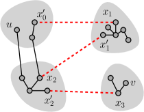
  Figure 3.4: Case II of the proof of Theorem 3.6. The grey blobs are supernodes in ${\mathscr{C}}$, the solid lines denote the forest $\mathscr{F}^{\star\star}$. The dotted lines are the path $P$. Observe we do not need to add the second edge of $P$ as it will create a cycle.

  How does the width of the trees in $\mathscr{F}^{\star\star}$ change? Each tree that we merge is inactive (since it is a coarsening of the original solution $\mathscr{F}^{\star}$). Connecting up $T_{1}^{\star\star},\ldots,T_{k}^{\star\star}$ causes the width of the resulting tree to be $\max\{0pt(T_{1}^{\star\star}),\cdots,0pt(T_{k}^{\star\star})\}$. The decrease in $0pt(\mathscr{F}^{\star\star})$ due to the merge is at least $\min\{0pt(T_{1}^{\star\star}),0pt(T_{2}^{\star\star})\}$, which ensures invariant (A) (using inequality (3.3)).

Hence, at the end of the run of gluttonous, both invariants hold. Since the initial potential is $0pt(\mathscr{F}^{\star})\leq\mathsf{cost}(\mathscr{F}^{\star})$, and the final potential is non-negative, the total cost of edges in $\mathscr{F}^{\star\star}\setminus\mathscr{F}^{\star}$ is at most $\mathsf{cost}(\mathscr{F}^{\star})$. This completes the proof. ∎

3.3 Charging to this Near-optimal Solution

Let $\mathscr{F}^{\star}=\{T^{\star}_{1},\ldots,T^{\star}_{p}\}$ be a solution to the Steiner forest instance. The main result of this section is:

Theorem 3.7

If the forest $\mathscr{F}^{\star}$ is faithful to the final clustering ${\mathscr{C}}^{f}$ of the gluttonous algorithm, then the cost of the gluttonous algorithm is $O(1)\cdot\mathsf{cost}(\mathscr{F}^{\star})$.

Since by Theorem 3.6 there is a forest $\mathscr{F}^{\star}$ with cost at most twice the optimum that is faithful to gluttonous’ final clustering ${\mathscr{C}}^{f}$, applying Theorem 3.7 to this forest proves Theorem 1.1.

We now prove Theorem 3.7. At a high level, the proof proceeds thus: we consider the run of the gluttonous algorithm, and maintain for each iteration $t$ a “candidate” forest ${\mathscr{F}}_{t}$ that is a solution to the remaining instance. We show that in an amortized sense, at each step the cost of forest ${\mathscr{F}}_{t}$ decreases by an amount which is a constant fraction of the cost incurred by gluttonous. Since the starting cost of this forest is at most a constant times the optimal cost, so is the total merging cost of the gluttonous, proving the result.

For Steiner forest instance ${\mathscr{I}}$, assume that ${\mathscr{C}}^{f}$ is gluttonous’ final clustering, and $\mathscr{F}^{\star}$ is faithful to ${\mathscr{C}}^{f}$. Let ${{\mathscr{C}}}^{(t)}$ be the gluttonous clustering at the beginning of the iteration $t$, with $\smash{{{\mathscr{C}}}^{(t)}_{{\small active}}}$ being the active supernodes. It will be useful to view this clustering as giving us an induced Steiner forest instance ${\mathscr{I}}_{t}$ on the metric whose points are the supernodes in ${{\mathscr{C}}}^{(t)}$ and where distances are given by the punctured metric $d_{{\mathcal{M}}/{{\mathscr{C}}}^{(t)}}$, where the terminals in the instance ${\mathscr{I}}_{t}$ are supernodes in $\smash{{{\mathscr{C}}}^{(t)}_{{\small active}}}$, and where active supernodes $\{S_{1},S_{2}\}$ are mates if there is a pair $\{u,\bar{u}\}$ such that $u\in S_{1}$ and $\bar{u}\in S_{2}$. (Supernodes no longer have unique mates, but this property was only used for convenience in Theorem 3.6). For any iteration $t$, the subsequent run of gluttonous is just a function of this induced instance ${\mathscr{I}}_{t}$. Indeed, given the instance ${\mathscr{I}}_{t}$, gluttonous outputs a final clustering which is same as ${\mathscr{C}}^{f}$ except the inactive supernodes in ${{\mathscr{C}}}^{(t)}$ are absent. I.e., the inactive supernodes in ${{\mathscr{C}}}^{(t)}$ will not play a role, but all the active supernodes will continue to combine in the same way in ${\mathscr{I}}_{t}$ as in ${\mathscr{I}}$. We now inductively maintain a forest ${\mathscr{F}^{(t)}}$ such that

• ${\mathscr{F}^{(t)}}$ is a feasible solution to this Steiner forest instance ${\mathscr{I}}_{t}$, and

• ${\mathscr{F}^{(t)}}$ maintains the connectivity structure of $\mathscr{F}^{\star}$, i.e., if $u$ and $v$ are two active terminals which are in the same tree in $\mathscr{F}^{\star}$, then the supernodes containing $u$ and $v$ lie in the same tree in ${\mathscr{F}^{(t)}}$.

And we will charge the cost of gluttonous to reductions in the cost of this forest ${\mathscr{F}^{(t)}}$.

The “candidate” forest ${\mathscr{F}^{(t)}}$.

The initial clustering ${{\mathscr{C}}}^{(1)}$ is the trivial clustering consisting of singleton terminals; we set ${\mathscr{F}^{(1)}}$ to $\mathscr{F}^{\star}$. Since ${\mathscr{I}}_{1}$ is the original instance, ${\mathscr{F}^{(1)}}$ is feasible for it; invariant (I2) is satisfied trivially.

For an iteration $t$, let $E({\mathscr{F}^{(t)}})$ denote the edges in ${\mathscr{F}^{(t)}}$. Note that an edge $e\in E({\mathscr{F}^{(t)}})$ between two supernodes $S_{1},S_{2}\in{{\mathscr{C}}}^{(t)}$ corresponds to an edge between two terminals $u,v$ in the original metric ${\mathcal{M}}$, where $u\in S_{1},v\in S_{2}$. Define $\mathsf{length}(e)$ as $d_{\mathcal{M}}(u,v)$, the length of the edge $e$ in the original metric. Note that the length of $e$ in the metric ${\mathcal{M}}/{{\mathscr{C}}}^{(t)}$ may be smaller than $\mathsf{length}(e)$. For every edge $e\in{\mathscr{F}^{(t)}}$, we shall also maintain a potential of $e$, denoted $\mathsf{\psi}(e)$. Initially, for $t=1$, the potential $\mathsf{\psi}(e)=\mathsf{length}(e)$ for all $e\in E({\mathscr{F}^{(1)}})$. During the course of the algorithm, the potential $\mathsf{\psi}(e)\geq\mathsf{length}(e)$; we describe the rule for maintaining potentials below. Intuitively, an edge $e\in{\mathscr{F}^{(t)}}$ would have been obtained by short-cutting several edges of $\mathscr{F}^{\star}$, and $\mathsf{\psi}(e)$ is equal to the total length of these edges.

Suppose we have a clustering ${{\mathscr{C}}}^{(t-1)}$ and a forest ${\mathscr{F}^{(t-1)}}$ which satisfies invariants (I1) and (I2). If we now merge two supernodes $S_{1},S_{2}\in{{\mathscr{C}}}^{(t-1)}$ to get clustering ${{\mathscr{C}}}^{(t)}$, we have to update the forest ${\mathscr{F}^{(t-1)}}$ to get to ${\mathscr{F}^{(t)}}$ using procedure UpdateForest given in Figure 3.5. The main idea is simple: when we merge the nodes corresponding to $S_{1}$ and $S_{2}$ in ${\mathscr{F}^{(t-1)}}$ into a single node, this creates a cycle. Removing any edge from the cycle maintains the invariants, and reduces the cost of the new forest: we remove the edge with the highest potential from the cycle. We further reduce the cost by getting rid of Steiner vertices, which correspond to inactive supernodes in ${\mathscr{F}^{(t)}}$ with degree 2. More formally, given two edges $e^{\prime}=\{u^{\prime},v\},e^{\prime\prime}=\{u^{\prime\prime},v\}$ with a common end-point $v$, the operation short-cut on $e^{\prime},e^{\prime\prime}$ replaces them by a single edge $\{u^{\prime},u^{\prime\prime}\}$. Whenever we see a Steiner vertex of degree 2 in ${\mathscr{F}^{(t)}}$, we shortcut the two incident edges.

Algorithm UpdateForest (${{\mathscr{C}}}^{(t-1)},S_{1},S_{2}$) : 1. Let $T$ be the tree in ${\mathscr{F}^{(t-1)}}$ containing the terminals in $S_{1}$ and $S_{2}$. 2. Merge $S_{1}$ and $S_{2}$ to a single node $S$ in the tree $T$. 3. If the new supernode $S$ becomes inactive, and has degree 2 in the tree $T$, then short-cut the two edges incident to $S$. 4. Let $C$ denote the unique cycle formed in the tree $T$. 5. Delete the edge in the cycle $C$ which has the highest potential. 6. While there is an inactive supernode in $T$ which is a degree-2 vertex, short-cut the two incident edges to this vertex.

Figure 3.5: The procedure for updating ${\mathscr{F}^{(t-1)}}$ to ${\mathscr{F}^{(t)}}$.

Some more comments about the procedure UpdateForest. In Step 1, the existence of the tree $T$ follows from the invariant property (I2) and the faithfulness of $\mathscr{F}^{\star}$ to ${\mathscr{C}}^{f}$. Since the terminals in $S_{1}\cup S_{2}$ are in the same tree in $\mathscr{F}^{\star}$, the invariant means they belong to the same tree in ${\mathscr{F}^{(t-1)}}$, and the construction ensures they remain in the same tree in ${\mathscr{F}^{(t)}}$. When we short-cut edges $e^{\prime},e^{\prime\prime}$ to get a new edge $e$, we define the potential of the new edge $e$ to be $\mathsf{\psi}(e):=\mathsf{\psi}(e^{\prime})+\mathsf{\psi}(e^{\prime\prime})$. It is also easy to check that ${\mathscr{F}^{(t)}}$ is a feasible solution to the instance ${\mathscr{I}}_{t}$. Indeed, the only difference between ${\mathscr{I}}_{t-1}$ and ${\mathscr{I}}_{t}$ is the replacement of $S_{1},S_{2}$ by $S$. If $S$ becomes inactive, there is nothing to prove. If $S$ remains active, then the tree containing $S$ must will also have also have the supernodes which were paired with $S_{1}$ and $S_{2}$ in the instance ${\mathscr{I}}_{t-1}$. It is also easy to check that the invariant property (I2) continues to hold. The following claim proves some more crucial properties of the forest ${\mathscr{F}^{(t)}}$.

Claim 3.8

For all iterations $t$, the Steiner nodes in ${\mathscr{F}^{(t)}}$ have degree at least 3. Therefore, there are at most 2 iterations of the while loop in Step 6 of the UpdateForest algorithm.

Proof.

We prove the first statement of the lemma by induction on $t$. For $t=1$, it holds by construction: we can assume that $\mathscr{F}^{\star}$ has no Steiner vertex of degree at most 2: any leaf Steiner node can be deleted, and a degree 2 can be removed by short-cutting the incident edges. Suppose this property is true for ${\mathscr{F}^{(t-1)}}$. We merge $S^{\prime}$ and $S^{\prime\prime}$, and if the new supernode $S$ becomes an inactive supernode, then its degree will be at least 2 (both $S^{\prime}$ and $S^{\prime\prime}$ must have had degree at least 1). If the degree is equal to 2, we remove this vertex in Step 3.

When we remove an edge in Step 5, the two end-points could have been Steiner vertices. By the induction hypothesis, their degree will be at least 2 (after the edge removal). If their degree is 2, we will again remove them by short-cutting edges. Note that this will not affect the degree of other nodes in the forest. This also shows that Step 6 will be carried out at most twice. ∎

Here’s the plan for rest of the analysis. Let’s fix a tree $T^{\star}$ of $\mathscr{F}^{\star}$, and account for only those merging costs which merge two supernodes with terminals in $T^{\star}$. (Summing over all trees in $\mathscr{F}^{\star}$ and using the faithfulness of $\mathscr{F}^{\star}$ to ${\mathscr{C}}^{f}$ will ensure all merging costs are accounted for.) Since ${\mathscr{F}^{(t)}}$ is obtained by repeatedly contracting nodes and removing unnecessary edges, in each iteration $t$ there is a unique tree ${T^{(t)}}$ in the forest ${\mathscr{F}^{(t)}}$ corresponding to the tree $T^{\star}$, namely the tree containing the active supernodes with terminals belonging to $T^{\star}$. Call an iteration of the gluttonous algorithm a relevant iteration (with respect to $T^{\star}$) if gluttonous merges two supernodes from the tree ${T^{(t)}}$ in this iteration. For brevity, we drop the phrase “w.r.t. $T^{\star}$” in the sequel.

Next we show that the total potential of the edges does not change over time. Let $\mathsf{del}(t)$ denote the set of edges which are deleted (from a cycle in Step 5) during the (relevant) iterations among $1,\ldots,t-1$. (Observe that $\mathsf{del}(t)$ does not include edges that are short-cut.)

Lemma 3.9

For iteration $t$, the sum of potentials of edges $\mathsf{del}(t)$ and $E({T^{(t)}})$ equals $\mathsf{cost}(T^{\star})$. Further, $\mathsf{\psi}(e)\geq\mathsf{length}(e)$ for all edges $e\in E({T^{(t)}})\cup\mathsf{del}(t)$.

Proof.

By induction on $t$. The base case $t=1$ follows by construction. For the IH, assume the statement holds for $t-1$. Assume that $t$ is a relevant iteration (else ${T^{(t)}}={T^{(t-1)}}$): if we remove edge $e$ from ${T^{(t-1)}}$ during Step 5, we do not change $\mathsf{\psi}(e)$. If we short-cut two edges $e^{\prime},e^{\prime\prime}$ to an edge $e$, $\mathsf{\psi}(e)=\mathsf{\psi}(e^{\prime})+\mathsf{\psi}(e^{\prime\prime})$. Therefore the total potential of the edges in the tree plus that of the edges in $\mathsf{del}(t)$ does not change. Further, $\mathsf{length}(e)\leq\mathsf{length}(e^{\prime})+\mathsf{length}(e^{\prime\prime})\leq\mathsf{\psi}(e^{\prime})+\mathsf{\psi}(e^{\prime\prime})=\mathsf{\psi}(e)$. ∎

Eventually ${T^{(t)}}$ has no active supernodes (for large $t$) and hence all its edges are deleted. Hence if $\mathsf{del}(\infty)$ denotes the edges deleted during all the relevant iterations in gluttonous, Lemma 3.9 implies $\sum_{e\in\mathsf{del}(\infty)}\mathsf{\psi}(e)=\mathsf{cost}(T^{\star})$. Let $\Delta_{t}$ denote the merging cost of some relevant iteration $t$: we now show how to charge this cost to the potential of some deleted edge in $\mathsf{del}(\infty)$. Formally, let $N_{t}$ denote the number of active supernodes in ${T^{(t)}}$, at the beginning of iteration $t$.

Theorem 3.10

If $t_{0}$ is relevant, there are at least $N_{t_{0}}/8$ edges in $\mathsf{del}(\infty)$ of potential at least $\Delta_{t_{0}}/6$.

We defer the proof of Theorem 3.10 for the moment, and instead show how to use this to charge the merging costs and to prove Theorem 3.7, which in turn gives the main theorem of the paper.

Proof of Theorem 3.7: Let $I^{r}$ denote the index set of all relevant iterations during the run of gluttonous. We now define a mapping $g$ from $I^{r}$ to $\mathsf{del}(\infty)$ such that: (i) for any edge $e\in\mathsf{del}(\infty)$, the pre-image $g^{-1}(e)$ has cardinality at most 8, and (ii) the potential $\mathsf{\psi}(g(t))\geq\Delta_{t}/6$ for all $t\in I^{r}$. To get this, consider a bipartite graph on vertices $I^{r}\cup\mathsf{del}(\infty)$ where a iteration $t\in I^{r}$ is connected to all edges $e\in\mathsf{del}(\infty)$ for which $\mathsf{\psi}(e)\geq\Delta_{t}/6$. Theorem 3.10 shows this graph satisfies a Hall-type condition for such a mapping to exist; in fact a greedy strategy can be used to construct the mapping (there can be at most $N_{t}$ relevant iterations after iteration $t$ because each relevant iteration reduces the number of active supernodes by at least one).

Thus, the total merging cost of gluttonous during relevant iterations is at most

$$\sum_{t\in I^{r}}\Delta_{t}=\sum_{e\in\mathsf{del}(\infty)}\sum_{t\in g^{-1}(e)}\Delta_{t}\leq 48\sum_{e\in\mathsf{del}(\infty)}\mathsf{\psi}(e)=48\,\mathsf{cost}(T^{\star}),$$

where the last equality follows from Lemma 3.9. By the faithfulness property, each iteration of gluttonous is relevant with respect to one of the trees in $\mathscr{F}^{\star}$, so summing the above expression over all trees gives the total merging cost to be at most $48\,\mathsf{cost}(\mathscr{F}^{\star})$. $\blacksquare$

Combining Theorem 3.7 with Theorem 3.6 gives an approximation factor of $96$ for the gluttonous algorithm. While we have not optimized the constants, but it is unlikely that our ideas will lead to constants in the single digits. Obtaining, for instance, a proof that the gluttonous algorithm is a $2$-approximation (or some such small constant) remains a fascinating open problem.

3.3.1 Proof of Theorem 3.10

In order to prove Theorem 3.10, we need to understand the structure of the trees ${T^{(t)}}$ for $t\geq t_{0}$ in more detail. Let $\mathsf{del}_{0}([t_{0}\ldots t))$ denote the edges deleted during the relevant iterations in $t_{0},\ldots,t-1$, i.e., $\mathsf{del}([t_{0}\ldots t)):=\mathsf{del}(t)\setminus\mathsf{del}(t_{0})$. Observe that each edge of ${T^{(t)}}$ is either in ${T^{(t_{0})}}$ or is obtained by short-cutting some set of edges of ${T^{(t_{0})}}$. Hence we maintain a partition ${\mathscr{E}}(t)$ of the edge set $E({T^{(t_{0})}})$, such that there is a correspondence between edges $e\in{T^{(t)}}\cup\mathsf{del}([t_{0}\ldots t))$ and sets $D_{t}(e)\in{\mathscr{E}}(t)$, such that $D_{t}(e)$ is the set of edges in ${T^{(t_{0})}}$ which have been short-cut to form $e$.

For each set $D_{t}(e)$, let $\mathsf{head}(D_{t}(e))$ be the edge $e^{\prime}\in D_{t}(e)$ with greatest length. If edge $e$ is removed from ${T^{(t)}}$ in some relevant iteration $t$, we have $e\in\mathsf{del}([t_{0}\ldots t^{\prime}))$ for all $t^{\prime}>t$, and the set $D_{t^{\prime}}(e)=D_{t}(e)$ for all future partitions ${\mathscr{E}}(t^{\prime})$.

Lemma 3.11

There are at least $N_{t_{0}}/2$ edges of length at least $\Delta_{t_{0}}/6$ in tree ${T^{(t_{0})}}$.

Proof.

Call an edge long if its length is at least $\Delta_{t_{0}}/6$, and let $\ell$ denote the number of long edges in the tree ${T^{(t_{0})}}$. Deleting these edges from ${T^{(t_{0})}}$ gives $\ell+1$ subtrees $C_{1},C_{2},\ldots,C_{l+1}$. Let $C_{i}$ have $n_{i}$ active supernodes and $e_{i}$ edges. For each tree $C_{i}$ where $n_{i}\geq 2$, take an Eulerian tour $X_{i}$ and divide it into $n_{i}$ disjoint segments by breaking the tour at the active supernodes. Each edge appears in two such segments, and each segment has at least six edges (since the distance between active supernodes is at least $\Delta_{t_{0}}$ and none of the edges are long), so $e_{i}\geq 3n_{i}$ when $n_{i}\geq 2$. This means the total number of edges in ${T^{(t_{0})}}$ is at least three times the number of “social” supernodes (supernodes that do not lie in a component $C_{i}$ with $n_{i}=1$, in which they are the only supernode), plus those $\ell$ long edges that were deleted.

And how many such social supernodes are there? If $\ell\geq N_{t_{0}}+1$, there may be none, but then we clearly have at least $N_{t_{0}}/2$ long edges. Else at least $N_{t_{0}}-\ell$ supernodes are social, so ${T^{(t_{0})}}$ has at least $3(N_{t_{0}}-\ell)+\ell$ edges. Finally, since every Steiner vertex in ${T^{(t_{0})}}$ has degree at least $3$, the number of edges is less than $2N_{t_{0}}$. Putting these together gives $3\,N_{t_{0}}-2\ell\leq 2\,N_{t_{0}}$ or $\ell\geq N_{t_{0}}/2$. ∎

Let $L_{0}$ be the set of long edges in ${T^{(t_{0})}}$, and ${\mathscr{E}}(\infty)$ be the partition at the end of the process. Two cases arise:

• At least $N_{t_{0}}/8$ edges in $L_{0}$ are $\mathsf{head}(D_{\infty}(e))$ for some set $D_{\infty}(e)\in{\mathscr{E}}(\infty)$. Since each set in ${\mathscr{E}}(\infty)$ has only one head, there are $N_{t_{0}}/8$ such sets. In any such set $D_{\infty}(e)$, $\mathsf{\psi}(e)\geq\mathsf{length}(\mathsf{head}(D_{\infty}(e)))\geq\Delta_{t_{0}}/6$. Moreover, we must have removed $e$ in some iteration between $t_{0}$ and the end, and hence $e\in\mathsf{del}([t_{0}\ldots\infty))\subseteq\mathsf{del}(\infty)$.

• More than than $3N_{t}/8$ edges in $L_{0}$ are not heads of any set in ${\mathscr{E}}(\infty)$. Take one such edge $e_{0}$ — the sets in ${\mathscr{E}}(t_{0})$ are singleton sets and hence $e_{0}$ is the head of the set $D_{t_{0}}(e_{0})$. Let $t$ be the first (relevant) iteration such that $e_{0}$ is not the head of the set containing it in ${\mathscr{E}}(t)$, and suppose $e_{0}=\mathsf{head}(D_{t-1}(e^{\prime}))$ for some set $D_{t-1}(e^{\prime})\in{\mathscr{E}}(t-1)$. In forming ${\mathscr{F}^{(t)}}$, we must have short-cut $e^{\prime}$ and some other edge $e^{\prime\prime}$ to form an edge $e\in{\mathscr{F}^{(t)}}$. Observe that $\mathsf{length}(\mathsf{head}(D(e^{\prime\prime}))\geq\mathsf{length}(e_{0})$, else $e_{0}$ would continue to be the head of $D(e)$. Moreover,

  $$\min\big{(}\mathsf{\psi}(e^{\prime}),\mathsf{\psi}(e^{\prime\prime})\big{)}\geq\min\big{(}\mathsf{length}(\mathsf{head}(e^{\prime})),\mathsf{length}(\mathsf{head}(e^{\prime\prime}))\big{)}\geq\Delta_{t_{0}}/6.$$

  By the discussion in Claim 3.8, one of $e^{\prime}$ and $e^{\prime\prime}$ must lie on the cycle formed when we merged two supernodes in ${\mathscr{F}^{(t-1)}}$, as in Step 4 of UpdateForest. Further, if $e_{t}$ was the edge removed from this cycle, by the rule in Step 5 we get that the potential $\mathsf{\psi}(e_{t})$ is the maximum potential of any edge on this cycle, and hence $\mathsf{\psi}(e_{t})\geq\min(\mathsf{\psi}(e^{\prime}),\mathsf{\psi}(e^{\prime\prime}))\geq\Delta_{t_{0}}/6$. Hence we want to “charge” this edge $e_{0}\in L_{0}$ to $e_{t}\in\mathsf{del}(\infty)$ (which has potential at least $\Delta_{t_{0}}/6$). However, up to three edges from $L_{0}$ may charge to $e_{t}$: this is because there can be at most three short-cut operations in any iteration (one from Step 3 and two from Step 6).

In both cases, we’ve shown the presence of at least $N_{t_{0}}/8$ edges in $\mathsf{del}(\infty)$ of potential $\Delta_{t_{0}}/6$, which completes the proof of Theorem 3.10.  

3.4 An Extension of the Analysis in Section 3

Let us now abstract out some properties used in the above analysis, so that we can generalize the analysis to a broader class of algorithms for Steiner forest. This abstraction is used to show that variants of the above algorithm, which are presented in Section 4 and in Appendix B, are also $O(1)$-approximations.

Consider an algorithm ${\mathscr{A}}$ which maintains a set of supernodes, where a supernode corresponds to a set of terminals, and two different supernodes correspond to disjoint terminals. Initially, we have one supernode for each terminal. Further, a supernode could be active or inactive. Once a supernode becomes inactive, it stays inactive. Now, at each iteration, the algorithm picks two active supernodes, and replaces them by a new supernode which is the union of the terminals in these two supernodes (the new supernode could be active or inactive). Note that the iteration when a supernode becomes inactive is arbitrary (depending on the algorithm ${\mathscr{A}}$).

As in the case of gluttonous algorithm, let ${\mathscr{C}}^{f}$ be the final clustering produced by the algorithm ${\mathscr{A}}$, and $T^{\star}$ be a tree solution to a Steiner forest instance $({\mathscr{D}},{\mathcal{M}})$. Let ${{\mathscr{C}}}^{(t)}$ be the set of supernodes at the beginning of iteration $t$ of ${\mathscr{A}}$. For an iteration $t$, let $\delta_{t}$ be the minimum distance (in the metric ${\mathcal{M}}/{{\mathscr{C}}}^{(t)}$) between any two active supernodes in ${{\mathscr{C}}}^{(t)}$. Claim 3.2 gives the following fact.

Fact 3.12

The quantity $\delta_{t}$ forms an ascending sequence with respect to $t$.

Now Theorem 3.7 generalizes to the following stronger result.

Corollary 3.13

For any tree solution $T^{\star}$ to an instance ${\mathscr{I}}$, $\sum_{t}\delta_{t}\leq 48\cdot\mathsf{cost}(T^{\star}).$

An important remark: this corollary is not making any claim about the merging cost of ${\mathscr{A}}$; at any iteration ${\mathscr{A}}$ could be connecting two active supernodes which are much farther apart than $\delta_{t}$.

4 A Timed Greedy Algorithm

We now give a version of the gluttonous algorithm TimedGlut where supernodes are deemed active or inactive based on the current time and not whether the terminals in the supernode have paired up with their mates. This version will be useful in getting a strict cost-sharing scheme.

The algorithm TimedGlut is very similar to the gluttonous algorithm except for what constitutes an active supernode.

We will again maintain a clustering of terminals (into supernodes) – let ${{\mathscr{C}}}^{(t)}$ be the clustering at the beginning of iteration $t$. Initially, at iteration $t=1$, ${{\mathscr{C}}}^{(1)}$ is the trivial clustering (consisting of singleton sets of terminals). We maintain a set of edges $E^{\prime}$ will be the set of edges bought by the algorithm. Initially, $E^{\prime}=\emptyset$.

We shall use $\Delta_{t}$ to denote the closest distance (in the metric ${\mathcal{M}}/{{\mathscr{C}}}^{(t)}$) between two active supernodes in ${{\mathscr{C}}}^{(t)}$. Our algorithm will only merge active supernodes, and an inactive supernode will not become active in future iterations. It follows that $\Delta_{t}$ cannot decrease with $t$ (Fact 3.1). This allows us to divide the execution of the algorithm into stages. Stage $i$ consists of those iterations $t$ for which $\Delta_{t}$ lies in the range $[2^{i},2^{i+1})$ (the initial stage belongs to stage 0, because we can assume w.l.o.g.  that the minimum distance between the terminals is 1).

For a terminal $s$, define

$$\mathsf{level}(s):=\lceil\log_{2}d_{\mathcal{M}}(s,{\bar{s}})\rceil.$$ (4.4)

Note that distances in this definition are measured in the original metric ${\mathcal{M}}$. For a supernode $S$, define its leader as the terminal in $S$ whose distance to its mate is the largest (and hence has the largest level); in case of ties, choose the terminal with the smallest index among these.

We shall use ${{\mathscr{C}}}^{i}$ to denote the clustering at the beginning of stage $i$ (note the change in notation with respect to the clustering at the beginning of an iteration $t$, which will be denoted by ${{\mathscr{C}}}^{(t)}$. So, if $t_{i}$ denotes the first iteration of stage $i$, then ${{\mathscr{C}}}^{i}$ is same as ${{\mathscr{C}}}^{(t_{i})}$). Now we specify when a supernode becomes inactive. A terminal $s$ is active at the beginning of stage $i$ if $\mathsf{level}(s)\geq i$. A supernode $S$ will be active at the beginning of a stage $i$ if $\mathsf{level}(\mathsf{leader}(S))\geq i$. Observe that supernodes do not become inactive during a stage – if a terminal is active at the beginning of a stage, it remains active during each of the iterations in this stage.

By the definition of a stage, the algorithm will satisfy the invariant that the distance between any two active supernodes in ${{\mathscr{C}}}^{i}$ (in the metric ${\mathcal{M}}/{{\mathscr{C}}}^{i}$) is at least $2^{i}$. During stage $i$, the algorithm repeatedly performs the following steps in each iteration $t$: pick any two arbitrary pair of active supernodes $S^{\prime},S^{\prime\prime}$ which are at most $2^{i+1}$ apart (in the metric ${\mathcal{M}}/{{\mathscr{C}}}^{(t)}$). Further, we take any such $S^{\prime}$-$S^{\prime\prime}$ path of length at most $2^{i+1}$ (in the graph induced by the metric ${\mathcal{M}}/{{\mathscr{C}}}^{(t)}$ on the vertex set ${{\mathscr{C}}}^{(t)}$) and add the edges (which go between supernodes) to $E^{\prime}$.

Stage $i$ ends when the merging distance between all remaining active supernodes is at least $2^{i+1}$. Observe that when the algorithm stops, we have a feasible solution—indeed, each terminal $s$ will merge with its mate ${\bar{s}}$ by the end of stage $\mathsf{level}(s)$. At the end, output a maximal acyclic subgraph of $E^{\prime}$.

The analysis of TimedGlut goes along the same lines as that of the gluttonous algorithm. The analog of Theorem 3.6 is as follows:

Theorem 4.1

Let $\mathscr{F}^{\star}=\{T_{1}^{\star},T_{2}^{\star},\ldots,T_{p}^{\star}\}$ be an optimal solution to the Steiner forest instance ${\mathscr{I}}=({\mathcal{M}},{\mathscr{D}})$. Let clustering ${\mathscr{C}}^{f}$ be produced by some run of the TimedGlut algorithm. There exists another solution $\mathscr{F}^{\star\star}$ for instance ${\mathscr{I}}$ such that

• $\mathsf{cost}(\mathscr{F}^{\star\star})\leq\mathsf{cost}(\mathscr{F}^{\star})+4\cdot 0pt(\mathscr{F}^{\star})\leq 5\cdot\mathsf{cost}(\mathscr{F}^{\star})$, and

• $\mathscr{F}^{\star\star}$ is faithful to the clustering ${\mathscr{C}}^{f}$.

Proof.

The proof is very similar to that of Theorem 3.6, where we look over the run of TimedGlut again to alter $\mathscr{F}^{\star}$ into $\mathscr{F}^{\star\star}$. Since TimedGlut makes some arbitrary choices, we make the same choices consistently in this proof. We ensure very similar invariants:

• The cost of edges in $\mathscr{F}^{\star\star}\setminus{\mathscr{F}}^{\star}$ is at most $4(0pt({\mathscr{F}}^{\star})-0pt(\mathscr{F}^{\star\star}))$, and

• at any point in time, the forest $\mathscr{F}^{\star\star}$ is faithful to the current clustering ${\mathscr{C}}$.

Observe the extra factor of $4$ in invariant (A). Again, let two active supernodes $S^{\prime}$ and $S^{\prime\prime}$ be merged in some stage $i$, and let $u$ and $v$ be the leaders of these supernodes respectively. The argument in Case I remains unchanged. In Case II, let $T_{1}^{\star\star}$ and $T_{2}^{\star\star}$ be the trees containing $u$ and $v$ respectively. Being in stage $i$, we know that $\mathsf{level}(u),\mathsf{level}(v)\geq i$, since they are both still active, and that the distance between $S^{\prime}$ and $S^{\prime\prime}$ in the current metric is at most $2^{i+1}$, since all merging costs in stage $i$ lie between $2^{i}$ and $2^{i+1}$. So the cost of connecting $T_{1}^{\star\star}$ and $T_{2}^{\star\star}$ is at most

$$2^{i+1}\leq\min(2^{\mathsf{level}(u)+1},2^{\mathsf{level}(v)+1}) \leq 4\cdot\min(d_{T_{1}^{\star\star}}(u,\bar{u}),d_{T_{2}^{\star\star}}(v,\bar{v}))$$

$$\leq 4\cdot\min(0pt(T_{1}^{\star\star}),0pt(T_{2}^{\star\star})).$$

The rest of the argument remains unchanged. ∎

Theorem 4.2

The TimedGlut algorithm is a $\gamma_{{\scriptscriptstyle TG}}$-approximation algorithm for Steiner forest, where $\gamma_{{\scriptscriptstyle TG}}=96\times 5=480$.

Proof.

Consider a solution $\mathscr{F}^{\star\star}$ which is faithful with respect to the final clustering produced by the TimedGlut algorithm. Suppose there are $m_{i}$ iterations during stage $i$. Then the total merging cost of the algorithm is at most $\sum_{i}2^{i+1}\cdot m_{i}$.

We would like to use Corollary 3.13. Let $\mathscr{F}^{\star\star}$ consist of the trees $\mathscr{T}^{\star\star}_{1},\ldots,\mathscr{T}^{\star\star}_{k}$. For a tree $\mathscr{T}^{\star\star}_{r}$, and a stage $i$, let $I_{i,r}$ denote the iterations when we merge two supernodes with terminals belonging to the tree $V(\mathscr{T}^{\star\star}_{r})$ (note that the faithfulness property implies that there will be such a tree for each iteration of the algorithm). Let $m_{i,r}$ denote the cardinality of $I_{i,r}$. Clearly, $\sum_{r}m_{i,r}=m_{r}$. For an iteration $t$, and index $r$, let ${{\mathscr{C}}}^{(t)}_{r}$ denote the supernodes in ${{\mathscr{C}}}^{(t)}$ with terminals belonging to $V(T^{\star}_{r})$. Define $\delta_{t,r}$ as the closest distance (in the metric ${\mathcal{M}}/{{\mathscr{C}}}^{(t)}$) between any two active supernodes with terminals belonging to $V(T^{\star}_{r})$. If the iteration belongs to stage $i$, then $\delta_{t,r}\geq 2^{i}$. Using Corollary 3.13, we get

$$\sum_{i}2^{i+1}m_{i}\leq 2\cdot\sum_{r}\sum_{i}2^{i}\cdot m_{i,r}\leq 98\cdot\sum_{r}\mathsf{cost}(T^{\star}_{r}).$$

The result now follows from Theorem 4.1. ∎

4.1 An Equivalent Description of TimedGlut

An essentially equivalent way to state the TimedGlut algorithm is as follows. For a stage $i$, let ${\mathcal{M}}_{i}$ denote the metric ${\mathcal{M}}/{{\mathscr{C}}}^{i}$ corresponding to the clustering at the beginning of stage $i$. Construct an auxiliary graph ${H^{(i)}}$ with vertex set being the set of supernodes in ${{\mathscr{C}}}^{i}$, and edges between two vertices if the two corresponding supernodes are active and the distance between them is at most $2^{i+1}$ in the metric ${\mathcal{M}}_{i}$. Pick a maximal acyclic set of edges ${{\cal P}^{(i)}}$ in this auxiliary graph ${H^{(i)}}$.

• For each edge $(S_{1},S_{2})\in{{\cal P}^{(i)}}$, merge the supernodes $S_{1},S_{2}$. Hence the clustering ${{\mathscr{C}}}^{i+1}$ at the end of stage $i$ is obtained by merging together all the supernodes that fall within a connected component of the subgraph $({H^{(i)}},{{\cal P}^{(i)}})$.

• For each edge $(S_{1},S_{2})\in{{\cal P}^{(i)}}$, add edges corresponding to a path of length $<2^{i+1}$ in ${\mathcal{M}}_{i}$ to a set of edges $E_{i}$.

Finally, output a maximal sub-forest of the edges $\cup_{i}E_{i}$ added during this process.

One can now check that this algorithm is equivalent to the TimedGlut algorithm as described above; the key observation is that because of the definition of the timed algorithm, an active terminal in stage $i$ stays active throughout the stage, and does not become inactive partway through it. More formally, we have the following observation.

Fact 4.3

Consider an execution of the TimedGlut algorithm on an input ${\mathscr{I}}$. Then one can define graphs ${H^{(i)}}$ and ${{\cal P}^{(i)}}$ for each stage $i$ such that the set of supernodes at the beginning of stage $i$ in the above algorithm is same as that of the TimedGlut algorithm. Further, the two algorithms pick the same set of edges in each stage.

5 Cost Shares for Steiner Forest

A cost-sharing method is a function $\chi$ mapping triples of the form $({\mathcal{M}},{\mathscr{D}},(s,{\bar{s}}))$ to the non-negative reals, where $({\mathcal{M}},{\mathscr{D}})$ is an instance of the Steiner forest problem, and $(s,{\bar{s}})\in{\mathscr{D}}$. We require the cost-sharing method to be budget-balanced: if $\mathscr{F}^{\star}$ is an optimal solution to the instance $({\mathcal{M}},{\mathscr{D}})$ then

$$\sum_{(s,{\bar{s}})\in{\mathscr{D}}}\chi({\mathcal{M}},{\mathscr{D}},(s,{\bar{s}}))\leq\mathsf{cost}(\mathscr{F}^{\star}).$$ (5.5)

We will consider strict cost-shares; these are useful for several problems in network design (see details in the introduction). There are two versions of strictness: uni-strictness, and strictness. Uni-strict cost-shares for Steiner forest were given by [GKPR07, FKLS10], whereas strict cost shares for Steiner forest have remained an open problem. We show how to get both using the TimedGlut algorithm.

5.1 Uni-strict Cost Shares for Steiner Forest

Definition 5.1

Given an $\alpha$-approximation algorithm ${\mathscr{A}}$ for the Steiner forest problem, a cost sharing $\chi$ is called $\beta$-uni-strict with respect to ${\mathscr{A}}$ if for all demand pair $(s,{\bar{s}})$, the cost share $\chi({\mathcal{M}},{\mathscr{D}},(s,{\bar{s}}))$ is at least $1/\beta$ times the distance between $s$ and $\bar{s}$ in the graph $G/F$, where $F$ is the forest returned by algorithm ${\mathscr{A}}$ on the input $({\mathcal{M}},{\mathscr{D}}-\{s,{\bar{s}}\})$.

Our objective is to find an algorithm ${\mathscr{A}}$ and the associated cost share $\chi$ such that the parameters $\alpha$ and $\beta$ are both constants.

5.1.1 Defining $\chi$ and ${\mathscr{A}}$

Let the constant $\gamma_{{\scriptscriptstyle TG}}$ denote the approximation ratio of the algorithm TimedGlut. The cost-sharing method is simple: for a terminal $s$, let $\ell_{s}$ be the largest value such that $s$ is a leader in stage $\ell_{s}$ and its supernode is merged with some other supernode during this stage (note that a supernode can go from being active in the beginning of a stage to becoming inactive in the next stage without merging with any supernode; this can happen because all terminals in it become inactive in the next stage). Then

$$\chi({\mathcal{M}},{\mathscr{D}},(s,{\bar{s}})):=\frac{2^{\ell_{s}}+2^{\ell_{\bar{s}}}}{2\gamma_{{\scriptscriptstyle TG}}}.$$ (5.6)

The algorithm ${\mathscr{A}}$ is a slight variant on the TimedGlut algorithm. Given an instance $({\mathcal{M}},{\mathscr{D}})$, run the algorithm TimedGlut on this instance to get forest $F$. Now merge some of the trees in $F$ as follows. Recall that the width of each tree $T$ in $F$ is defined to be $0pt(T):=\max_{(s,{\bar{s}})\in T}d_{T}(s,{\bar{s}})$, where $d_{T}(s,{\bar{s}})$ denotes the distance between $s$ and $\bar{s}$ in the tree $T$. While there are trees $T_{1},T_{2}\in F$ such that $d_{{\mathcal{M}}/F}(T_{1},T_{2})\leq 5\min(0pt(T_{1}),0pt(T_{2}))$, connect $T_{1},T_{2}$ by a path of length $d_{{\mathcal{M}}/F}(T_{1},T_{2})$ to get a tree $T$, and update $F\leftarrow(F\setminus\{T_{1},T_{2}\})\cup\{T\}$. Here, $d_{{\mathcal{M}}/F}(T_{1},T_{2})$ denotes the minimum over all pairs $u\in T_{1},v\in T_{2},$ of $d_{{\mathcal{M}}/F}(u,v)$.

5.1.2 Analysis

We now prove that the cost sharing method $\chi$ is $\beta$-uni-strict with respect to ${\mathscr{A}}$, where $\beta$ is a constant. Recall that $F$ denotes the forest returned by the algorithm ${\mathscr{A}}$.

To begin, observe that the algorithm ${\mathscr{A}}$ is also a constant-factor approximation.

Lemma 5.2

The algorithm ${\mathscr{A}}$ is an $6\gamma_{{\scriptscriptstyle TG}}$-approximation for Steiner forest.

Proof.

Let $F^{\prime}$ be the forest returned by the TimedGlut algorithm (called by ${\mathscr{A}}$). Consider the potential $\sum_{T\in F^{\prime}}(c(T)+5\,0pt(T))$. Since the width of each tree is at most the cost of its edges, and since TimedGlut was a $\gamma_{{\scriptscriptstyle TG}}$-approximation, this potential is at most $6\gamma_{{\scriptscriptstyle TG}}$ times the optimal cost. Now, observe that whenever ${\mathscr{A}}$ merges two trees of this forest, the potential of the new forest does not increase. Therefore, the potential of the forest $F$ is also at most $6\gamma_{{\scriptscriptstyle TG}}$ times the optimal cost. ∎

Lemma 5.3

The function $\chi$ is a budget-balanced cost sharing method.

Proof.

We need to prove the inequality (5.5). To do this, let us run TimedGlut and “charge” the cost of merging two active supernodes to the leaders of the respective clusters—charge half of the distance between these two supernodes to the leaders of each of these supernodes. Clearly, the total charge assigned to the terminals is equal to the total cost paid by the algorithm TimedGlut, which at most $\gamma_{{\scriptscriptstyle TG}}\,\mathsf{cost}(\mathscr{F}^{\star})$. Finally, we make the observation that each terminal $s$ is charged at least $\gamma_{{\scriptscriptstyle TG}}$ times the cost share (since it is charged at least $2^{\ell_{s}}/2$ in stage $\ell_{s}$) to complete the proof. ∎

To prove the uni-strictness property, fix a terminal pair $(s,{\bar{s}})$, and consider two instances: ${\mathscr{I}}=({\mathcal{M}},{\mathscr{D}})$ and ${\mathscr{I}}^{\prime}=({\mathcal{M}},{\mathscr{D}}-\{(s,{\bar{s}})\})$. For instance ${\mathscr{I}}$, let ${{\mathscr{C}}}^{i}$ denote the set of supernodes at the beginning of stage $i$; let ${{\mathscr{C}}}^{{}^{\prime}i}$ be the corresponding set for ${\mathscr{I}}^{\prime}$. Let ${\mathcal{M}}_{i}$ and ${\mathcal{M}}_{i}^{\prime}$ denote the metrics ${\mathcal{M}}/{{\mathscr{C}}}^{i}$ and ${\mathcal{M}}/{{\mathscr{C}}}^{{}^{\prime}i}$ respectively. Recall that $\mathsf{level}(s)=\lceil\log_{2}d_{\mathcal{M}}(s,{\bar{s}})\rceil$.

The following claim will be convenient to understand the behavior of TimedGlut.

Lemma 5.4

Consider stage $i$ in the execution TimedGlut on the instance ${\mathscr{I}}$. Define a graph ${\mathscr{G}}_{i}$ on the vertex set ${{\mathscr{C}}}^{i}$, with an edge between two active supernodes $C_{1},C_{2}\in{{\mathscr{C}}}^{i}$ if there is a path of length at most $2^{i+1}$ between them in ${\mathcal{M}}_{i}$ that does not contain any other active supernode as an internal node. If the connected components of ${\mathscr{G}}_{i}$ are $H_{1},\ldots,H_{q}$, then ${{\mathscr{C}}}^{i+1}$ has $q$ supernodes—one supernode for each $H_{j}$ (formed by merging the supernodes in $H_{j}$).

Proof.

The statement is essentially the same as Fact 4.3 except that in the graph ${H^{(i)}}$ (defined in Section 4.1), we join two active supernodes $C_{1},C_{2}\in{{\mathscr{C}}}^{i}$ by an edge if the distance between them in the metric ${\mathcal{M}}_{i}$ is at most $2^{i+1}$, whereas here in the graph ${\mathscr{G}}_{i}$, we wish to have a path of length at most $2^{i+1}$ with no internal vertex being an active supernode. We claim that the connected components in the two graphs are the same, and hence, the statement in the lemma follows.

Clearly, an edge $e\in{\mathscr{G}}_{i}$ is present in ${H^{(i)}}$ as well. Now, consider an edge $(C_{1},C_{2})$ in ${H^{(i)}}$. Let $P$ be the shortest path of length at most $2^{i+1}$ between $S_{1}$ and $S_{2}$ in the metric ${\mathcal{M}}_{i}$. Let the active supernodes on this path be $C_{1}=C_{i_{1}},C_{i_{2}},\ldots,C_{i_{p}}=C_{2}$ (in this order). Then ${\mathscr{G}}_{i}$ has edges $(C_{i_{r}},C_{i_{r+1}})$ for $r=1,\ldots,p-1$. Therefore $C_{1}$ and $C_{2}$ are in the same connected component of ${\mathscr{G}}_{i}$. This proves the desired claim. ∎

Theorem 5.5 (Nesting)

For $i\leq\mathsf{level}(s)$, let $C_{s}$ and $C_{\bar{s}}$ be the supernodes in ${{\mathscr{C}}}^{i}$ containing $s$ and $\bar{s}$ respectively. The following hold:

1. If $C_{s}\neq C_{\bar{s}}$, we can arrange the supernodes in ${{\mathscr{C}}}^{{}^{\prime}i}$ as $C_{1}^{\prime},\ldots,C_{p}^{\prime}$ such that $C_{s}=\{s\}\cup C_{1}^{\prime}\cup\ldots\cup C_{a}^{\prime},$ $C_{\bar{s}}=\{\bar{s}\}\cup C_{a+1}^{\prime}\cup\ldots\cup C_{b}^{\prime}$ for some $0\leq a\leq b\leq p$. Moreover, ${{\mathscr{C}}}^{i}-\{C_{s},C_{\bar{s}}\}=\{C_{b+1}^{\prime},\ldots,C_{p}^{\prime}\}$. If $C_{s}=C_{\bar{s}}$, we can arrange the supernodes in ${{\mathscr{C}}}^{{}^{\prime}i}$ as $C_{1}^{\prime},\ldots,C_{p}^{\prime}$ such that $C_{s}=\{s,{\bar{s}}\}\cup C_{1}^{\prime}\cup\ldots\cup C_{b}^{\prime},$ for some $0\leq b\leq p$. Also, ${{\mathscr{C}}}^{i}-\{C_{s}\}=\{C_{b+1}^{\prime},\ldots,C_{p}^{\prime}\}$.

2. Suppose $C_{s}$ and $C_{\bar{s}}$ are distinct supernodes. Then for any terminal $v\in C_{s}$, $d_{{\mathcal{M}}^{\prime}_{i}}(s,v)\leq 2\cdot 2^{i}$. Similarly, for any $v\in C_{\bar{s}}$, $d_{{\mathcal{M}}^{\prime}_{i}}(\bar{s},v)\leq 2\cdot 2^{i}$.

3. Suppose $C_{s}=C_{\bar{s}}$. Then, $d_{{\mathcal{M}}^{\prime}_{i}}(s,{\bar{s}})\leq 4\cdot 2^{i}$.

Proof.

We induct on $i$. At the beginning, all clusters are singletons, so the base case is easy. For the inductive step, suppose the statement of the theorem is true for some $i<\mathsf{level}(s)$. Assume that $C_{s}\neq C_{\bar{s}}$, the other case is similar. Apply Lemma 5.4 to stage $i$ in both ${\mathscr{I}}$ and ${\mathscr{I}}^{\prime}$, and let ${\mathscr{G}}_{i}$ and ${\mathscr{G}}_{i}^{\prime}$ be the corresponding graphs on the vertex sets ${{\mathscr{C}}}^{i}$ and ${{\mathscr{C}}}^{{}^{\prime}i}$ (as defined in Lemma 5.4). We know that the supernodes of ${{\mathscr{C}}}^{i+1}$ and ${{\mathscr{C}}}^{{}^{\prime}i+1}$ correspond to the connected components of these graphs; we now use this information to prove the induction step.

By the induction hypothesis, the supernodes in ${{\mathscr{C}}}^{i}$ can be labeled $C_{s},C_{\bar{s}},C_{b+1}^{\prime},\ldots,C_{p}^{\prime}$; moreover, we can define a map $\phi:V({\mathscr{G}}_{i}^{\prime})\to V({\mathscr{G}}_{i})$ as follows:

$$\phi(C_{j}^{\prime}):=\begin{cases}C_{s}&0\leq j\leq a\\ C_{\bar{s}}&a+1\leq j\leq b\\ C_{j}^{\prime}\quad&b+1\leq j\leq p\end{cases}$$ (5.7)

Suppose there is an edge between $C_{j}^{\prime}$ and $C_{k}^{\prime}$ in ${\mathscr{G}}_{i}^{\prime}$. By the definition of ${\mathscr{G}}_{i}$, both are active supernodes, and the length of the shortest path between them in the metric ${\mathcal{M}}_{i}^{\prime}$ is at most $2^{i+1}$. This path has no greater length in the metric ${\mathcal{M}}_{i}$, since the supernodes in ${{\mathscr{C}}}^{i}$ are unions of supernodes in ${{\mathscr{C}}}^{{}^{\prime}i}$. This means there is a path between $\phi(C_{j}^{\prime})$ and $\phi(C_{k}^{\prime})$ in ${\mathscr{G}}_{i}$, i.e., the clustering ${{\mathscr{C}}}^{{}^{\prime}i+1}$ is a refinement of ${{\mathscr{C}}}^{i+1}$ (because these clusterings are determined by the connected components of the corresponding graphs).

Now consider an edge $e$ in ${\mathscr{G}}_{i}$. For the first part of the theorem, suppose $e=(C_{j}^{\prime},C_{k}^{\prime})$ where both $j,k\geq b+1$. If $P$ is the corresponding path in ${\mathcal{M}}_{i}$ between these two supernodes, then $P$ cannot contain $C_{s}$ or $C_{\bar{s}}$ as an internal node (because it does not contain any active supernodes as internal nodes, and both $C_{s},C_{\bar{s}}$ are active). But then the length of $P$ remains unchanged in ${\mathcal{M}}_{i}^{\prime}$, and we have the corresponding edge $(C_{j}^{\prime},C_{k}^{\prime})$ in ${\mathscr{G}}_{i}^{\prime}$ as well. This means that all the connected components of ${\mathscr{G}}_{i}$ not containing $C_{s}$ or $C_{\bar{s}}$ also form connected components in ${\mathscr{G}}_{i}^{\prime}$. Combined with the fact that ${{\mathscr{C}}}^{{}^{\prime}i+1}$ is a refinement of ${{\mathscr{C}}}^{i+1}$, this proves the part (a) of the theorem for the case $C_{s}\neq C_{\bar{s}}$. (The proof for the other case is similar.)

For part (b), let $H_{1}$ be the connected component of ${\mathscr{G}}_{i}$ which contains the supernode $C_{s}$ (as a vertex). So all the supernodes in $H_{1}$ will merge to form a single supernode of ${{\mathscr{C}}}^{i+1}$. As argued in the paragraph above, any edge in $H_{1}$ which is not incident with $C_{s}$ is also present in ${\mathscr{G}}_{i}^{\prime}$(recall that we are assuming $C_{\bar{s}}$ is not one of the vertices in $H_{1}$). Let $v$ be a terminal in a supernode $B$ in $H_{1}$. Let the path from $C_{s}$ to $B$ in $H_{1}$ be $C_{s}=A_{0},A_{1},\ldots,A_{r}=B$. Since the edges $(A_{1},A_{2}),\ldots,(A_{r-1},A_{r})$ belong to ${\mathscr{G}}_{i}^{\prime}$ as well, $A_{1},\ldots,A_{r}$ will lie in the same supernode in ${{\mathscr{C}}}^{{}^{\prime}i+1}$. Therefore, $d_{{\mathcal{M}}_{i+1}^{\prime}}(s,v)\leq 2^{i+1}+2\cdot 2^{i}=2\cdot 2^{i+1}$, where the term $2\cdot 2^{i}$ is present to account for the distance between $s$ and the terminal in $C_{s}$ which is closest to $A_{1}$ – this distance can be at most $2\cdot 2^{i}$ by the induction hypothesis.

For part (c), consider the last stage $i$ such that the supernodes $C_{s}$ and $C_{\bar{s}}$ are distinct (so the result in part (b) applies to this stage). The same argument as above applies except that when we consider the path from $C_{s}$ to $C_{\bar{s}}$ in the component of ${\mathscr{G}}_{i}$ containing them, we will have to account for the first and the last edges in this path. ∎

We are now ready to prove the uni-strictness of the cost-shares. We run TimedGlut on the instance ${\mathscr{I}}$ to get the cost shares, and let the cost share for $(s,\bar{s})$ be as in (5.6). Now let $F^{\prime}$ be the forest returned by the algorithm ${\mathscr{A}}$ on the instance ${\mathscr{I}}^{\prime}$. Recall that ${\mathcal{M}}/F^{\prime}$ denotes the metric ${\mathcal{M}}$ with the connected components in $F^{\prime}$ contracted to single points.

Lemma 5.6

The distance between $s$ and $\bar{s}$ in ${\mathcal{M}}/F^{\prime}$ is at most $4\cdot(2^{\ell_{s}+1}+2^{\ell_{\bar{s}}+1})$.

Proof.

Let $j:=\max(\ell_{s},\ell_{\bar{s}})+1$. Suppose $j\geq\mathsf{level}(s)$, then the claim is trivial because $d_{\mathcal{M}}(s,\bar{s})\leq 2^{\mathsf{level}(s)}\leq 2^{j}\leq 2\cdot(2^{\ell_{s}}+2^{\ell_{\bar{s}}})$; hence consider the case where $j\leq\mathsf{level}(s)-1$.

Let $C_{s}$ and $C_{\bar{s}}$ denote the supernodes containing $s$ and $\bar{s}$ in clustering ${{\mathscr{C}}}^{j}$ respectively. There are two cases. The first case is when $C_{s}$ is same as $C_{\bar{s}}$. In this case, part (c) of Theorem 5.5 implies that $\smash{d_{{\mathcal{M}}^{\prime}_{j}}(s,\bar{s})}\leq 4\cdot 2^{j}\leq 4\cdot(2^{\ell_{s}+1}+2^{\ell_{\bar{s}}+1})$. The distance in metric $d_{{\mathcal{M}}/F^{\prime}}$ can only be smaller.

The other case is when $C_{s}$ and $C_{\bar{s}}$ are different. Note that $C_{s}$ will be merged with another supernode in some stage during or after stage $j$ (eventually the $s$ and ${\bar{s}}$ will end up in the same supernode). Since $j>\ell_{s}$, it follows from the definition of $\ell_{s}$ that $s$ is not the leader of $C_{s}$. Similarly, ${\bar{s}}$ is not the leader of $C_{\bar{s}}$. Let the leaders of $C_{s}$ and $C_{\bar{s}}$ be $v_{1}$ and $v_{2}$ respectively. By Theorem 5.5(b), we know that $\smash{d_{{\mathcal{M}}^{\prime}_{j}}(s,v_{1})}\leq 2\cdot 2^{j}$ and $d_{{\mathcal{M}}^{\prime}_{j}}({\bar{s}},v_{2})\leq 2\cdot 2^{j}$. Consequently,

$$d_{{\mathcal{M}}^{\prime}_{j}}(v_{1},v_{2})\leq d_{{\mathcal{M}}^{\prime}_{j}}(v_{1},s)+d_{{\mathcal{M}}^{\prime}_{j}}(s,\bar{s})+d_{{\mathcal{M}}^{\prime}_{j}}({\bar{s}},v_{2})\leq 4\cdot 2^{j}+d_{\mathcal{M}}(s,\bar{s})\leq 5\,d_{\mathcal{M}}(s,\bar{s}),$$

where the last inequality follows because $d_{{\mathcal{M}}}(s,\bar{s})\geq d_{{\mathcal{M}}_{j}}(C_{s},C_{\bar{s}})\geq 2^{j}$.

Let $F^{\prime\prime}$ be the final forest produced by TimedGlut on the instance ${\mathscr{I}}^{\prime}$; recall that $F^{\prime}$ is obtained from $F^{\prime\prime}$ by merging together some of these trees. Let $T_{1}$ and $T_{2}$ be the trees in $F^{\prime\prime}$ which contain $v_{1}$ and $v_{2}$ respectively. Since the distance between $v_{1}$ and $v_{2}$ is already at most $5\,d_{\mathcal{M}}(s,\bar{s})$ at the beginning of stage $j$, we know that $d_{{\mathcal{M}}/F^{\prime}}(T_{1},T_{2})\leq 5\,d_{\mathcal{M}}(s,\bar{s})$, where ${\mathcal{M}}/F^{\prime}$ denotes the metric $M$ with the trees in $F^{\prime}$ contracted.

Since $s$ lost its leadership to $v_{1}$, it must be the case that $d(s,{\bar{s}})\leq d(v_{1},{\bar{v_{1}}})$; thus $0pt(T_{1})\geq d(s,\bar{s})$; a similar argument shows $0pt(T_{2})\geq d(s,\bar{s})$. Since $d_{{\mathcal{M}}/F^{\prime}}(T_{1},T_{2})\leq 5\,\min(0pt(T_{1}),0pt(T_{2}))$, the algorithm ${\mathscr{A}}$ would have merged $T_{1}$ and $T_{2}$ into one tree. This makes the distance $d_{{\mathcal{M}}/F^{\prime}}(v_{1},v_{2})=0$ and hence

$$d_{{\mathcal{M}}/F^{\prime}}(s,\bar{s})\leq d_{{\mathcal{M}}/F^{\prime}}(s,v_{1})+d_{{\mathcal{M}}/F^{\prime}}(v_{2},{\bar{s}})\leq d_{{\mathcal{M}}/{{\mathscr{C}}}^{j}}(s,v_{1})+d_{{\mathcal{M}}/{{\mathscr{C}}}^{j}}({\bar{s}},v_{2})\leq 4\cdot 2^{j},$$

proving the claim. ∎

This shows that the cost of connecting $(s,\bar{s})$ in ${\mathcal{M}}/F^{\prime}$ is at most $\beta:=16\gamma_{{\scriptscriptstyle TG}}$ times the cost share of $(s,\bar{s})$, which proves the uni-strictness property.

5.2 Strict Cost Shares

We now extend the previous cost sharing scheme to the more general strict cost sharing scheme. Let $\chi$ be a budget-balanced cost sharing function for the Steiner forest problem. As before, let ${\mathscr{A}}$ be an $\alpha$-approximation algorithm for the Steiner forest problem.

Definition 5.7

A cost-sharing function $\chi$ is $\beta$-strict with respect to an algorithm ${\mathscr{A}}$ if for all pairs of disjoint terminal sets ${\mathscr{D}}_{1},{\mathscr{D}}_{2}$ lying in a metric ${\mathcal{M}}$, the following condition holds: if ${\mathscr{D}}$ denotes ${\mathscr{D}}_{1}\cup{\mathscr{D}}_{2}$, then $\sum_{(s,{\bar{s}})\in{\mathscr{D}}_{2}}\chi({\mathcal{M}},{\mathscr{D}},(s,{\bar{s}}))$ is at least $1/\beta$ times the the cost of the optimal Steiner forest on ${\mathscr{D}}_{2}$ in the metric ${\mathcal{M}}/F$, where $F$ is the forest returned by ${\mathscr{A}}$ on the input $({\mathcal{M}},{\mathscr{D}}_{1})$.

In addition to the TimedGlut algorithm, we will also need a timed primal-dual algorithm for Steiner forest, denoted by TimedPD. The input for the TimedPD algorithm is a set of terminals, each terminal $s$ being assigned an activity time $\mathsf{time}(s)$ such that the terminal is active for all times $t\leq\mathsf{time}(s)$. The primal-dual algorithm grows moats around terminals as long as they are active and buys edges that ensure that if two moats meet at some time $t$, all the terminals in these moats that are active at time $t$ lie in the same tree. One can do this in different ways (see, e.g., [GKPR07, Pál04, KLS05]); for concreteness we refer to the KLS algorithm of Könemann et al. [KLS05] which gives the following guarantee:

Theorem 5.8

If $\mathsf{time}(s)=\frac{1}{2}d_{\mathcal{M}}(s,\bar{s})$ for all terminals $s$, then the total cost of edges bought by the timed primal-dual algorithm KLS is at most $2\cdot\mathsf{opt}({\mathscr{I}})$.

The following property can be shown for the KLS algorithm:

Lemma 5.9

Multiplying the activity times by a factor of $K\geq 1$ to $\frac{K}{2}\cdot d_{\mathcal{M}}(s,\bar{s})$ causes the KLS algorithm to output another feasible solution of total cost at most $2K\cdot\mathsf{opt}({\mathscr{I}})$.

5.2.1 Defining $\chi$ and ${\mathscr{A}}$

Defining $\chi$ and ${\mathscr{A}}$

To define the cost-shares for the instance ${\mathscr{I}}=({\mathcal{M}},{\mathscr{D}})$, run the algorithm TimedGlut on ${\mathscr{I}}$. Recall the description of the algorithm as given in §​ 4.1: in each stage $i$, we choose a collection ${{\cal P}^{(i)}}$ of pairs of supernodes whose mutual distance (in the metric ${\mathcal{M}}/{{\mathscr{C}}}^{i}$) lies in the range $[2^{i},2^{i+1})$, merge each such pair of supernodes to get the new clustering (and add edges in the underlying graph of at most as much length). For pair $(S,S^{\prime})\in{{\cal P}^{(i)}}$, if $s,s^{\prime}$ are the leaders of $S,S^{\prime}$ respectively, increment the cost-share of each of $(s,\bar{s})$ and $(s^{\prime},\bar{s}^{\prime})$ by $\frac{2^{i+1}}{2\gamma_{{\scriptscriptstyle TG}}}$. Since the analysis of the TimedGlut algorithm proceeds by showing that the quantity $\sum_{i}|{{\cal P}^{(i)}}|\cdot 2^{i+1}\leq\gamma_{{\scriptscriptstyle TG}}\,\mathsf{opt}({\mathscr{I}})$, the budget-balance property follows.

The algorithm ${\mathscr{A}}$ on input ${\mathscr{I}}=({\mathcal{M}},{\mathscr{D}})$ is simple: set the activity time $\mathsf{time}(s):=6\cdot 2^{\mathsf{level}(s)+1}$ for each terminal $s$, and run the algorithm TimedPD. The following claim immediately follows from Lemma 5.9 and Theorem 5.8, and the fact that $6\cdot 2^{\mathsf{level}(s)+1}\leq 12\cdot 2^{2}\cdot\frac{1}{2}d_{\mathcal{M}}(s,\bar{s})$.

Lemma 5.10

The algorithm ${\mathscr{A}}$ is a $96$-approximation algorithm for Steiner forest.

5.2.2 Proving Strictness

Given a set of demands ${\mathscr{D}}$ in a metric space ${\mathcal{M}}$, and a partition into ${\mathscr{D}}_{1}\cup{\mathscr{D}}_{2}$, we run the algorithm ${\mathscr{A}}$ on ${\mathscr{D}}_{1}$—let $F_{1}$ be the forest returned by this algorithm, and let metric ${\mathcal{M}}_{1}$ be obtained by contracting the edges of $F_{1}$. To prove the strictness property, we now exhibit a “candidate” Steiner forest $F_{2}$ for ${\mathscr{D}}_{2}$ in the metric ${\mathcal{M}}_{1}$ with cost at most a constant factor times $\sum_{(s,{\bar{s}})\in{\mathscr{D}}_{2}}\chi({\mathcal{M}},{\mathscr{D}},(s,{\bar{s}})),$ the total cost-share assigned to the terminals in ${\mathscr{D}}_{2}$.

Recall that the algorithm ${\mathscr{A}}$ on ${\mathscr{D}}_{1}$ is just the TimedPD algorithm. We divide this algorithm’s run into stages, where the $i^{th}$ stage lasts for the time interval $[6\cdot 2^{i},6\cdot 2^{i+1})$; the $0^{th}$ stage lasts for $[0,6\cdot 2)$. Let $\smash{F_{1}^{(i)}}$ be the edges of the output forest $F_{1}$ which become tight during stage $i$ of this run, and ${\mathfrak{M}_{1}^{(i)}}$ be the set of moats at the beginning of stage $i$. These moats are defined in the original metric ${\mathcal{M}}$.

Defining a Candidate Forest $F_{2}$

To define the forest $F_{2}$ connecting ${\mathscr{D}}_{2}$, we now imagine running TimedGlut on the entire demand set ${\mathscr{D}}_{1}\cup{\mathscr{D}}_{2}$ on the original metric ${\mathcal{M}}$, look at paths added by that algorithm, and choose a carefully chosen subset of these paths to add to $F_{2}$. This is the natural thing to do, since such a run of TimedGlut was used to define the cost-shares $\chi$ in the first place. Recall the description of TimedGlut from §​ 4.1, and let ${\mathcal{R}}$ denote this run of TimedGlut on ${\mathscr{I}}=({\mathcal{M}},{\mathscr{D}}_{1}\cup{\mathscr{D}}_{2})$.

We examine the run ${\mathcal{R}}$ stage by stage: at the beginning of stage $i$, the run ${\mathcal{R}}$ took the current clustering ${{\mathscr{C}}}^{i}$, built an auxiliary graph ${H^{(i)}}$ whose nodes were the supernodes in ${{\mathscr{C}}}^{i}$ and edges were pairs of active supernodes that had mutual merging distance at most $2^{i+1}$, picked some maximal forest ${{\cal P}^{(i)}}$ in this graph, merged these supernode pairs in ${{\cal P}^{(i)}}$, and bought edges in the underlying metric corresponding to paths connecting these supernode pairs. We show how to choose some subset of these underlying edges to add to our candidate forest—we denote these edges by $\smash{F_{2}^{(i)}}$.

In the following, we will talk about edges $(S,S^{\prime})\in{{\cal P}^{(i)}}$ (which are edges of the auxiliary graph ${H^{(i)}}$) and edges in the metric ${\mathcal{M}}$. To avoid confusion, we refer to $(S,S^{\prime})$ as pairs and those in the metric as edges.

What edges should we add to $\smash{F_{2}^{(i)}}$? For that, look at the end of stage $i$ of the run of ${\mathscr{A}}$ on ${\mathscr{D}}_{1}$; the primal-dual algorithm has formed a set of moats ${\mathfrak{M}_{1}^{(i+1)}}$ at this point. We define an equivalence relation on the supernodes in ${{\mathscr{C}}}^{i}$ as follows. If the leaders of two supernodes $S,S^{\prime}\in{{\mathscr{C}}}^{i}$ both lie in ${\mathscr{D}}_{1}$, and also in the same moat of ${\mathfrak{M}_{1}^{(i+1)}}$, we put $S$ and $S^{\prime}$ in the same equivalence class. Now if we collapse each equivalence class by identifying all the supernodes in that class, the pairs in ${{\cal P}^{(i)}}$ may no longer be acyclic in the collapsed version of ${H^{(i)}}$, they may contain cycles and self-loops. Consider a maximal acyclic set of pairs in ${{\cal P}^{(i)}}$, and denote the dropped pairs by $\smash{{\cal P}_{X}^{(i)}}$. The set ${{\cal P}^{(i)}}$ is now classified into three parts (see Figure 5.6 for an example):

• Let ${{\cal P}_{G}^{(i)}}$ be pairs $(S,S^{\prime})\in{{\cal P}^{(i)}}\setminus\smash{{\cal P}_{X}^{(i)}}$ for which at least one of $\mathsf{leader}(S),\mathsf{leader}(S^{\prime})$ belongs to ${\mathscr{D}}_{2}$.

• Let $\smash{{\cal P}_{B}^{(i)}}$ be pairs $(S,S^{\prime})\in{{\cal P}^{(i)}}\setminus\smash{{\cal P}_{X}^{(i)}}$ for which both of $\mathsf{leader}(S)$ and $\mathsf{leader}(S^{\prime})$ belongs to ${\mathscr{D}}_{1}$.

• Of course, $\smash{{\cal P}_{X}^{(i)}}$ is the set of pairs $(S,S^{\prime})\in{{\cal P}^{(i)}}$ dropped to get an acyclic set.

Given this classification, the edges we add to $\smash{F_{2}^{(i)}}$ are as follows. Recall that in the run ${\mathcal{R}}$, for each pair $(S,S^{\prime})\in{{\cal P}^{(i)}}$, we had added edges connecting those two supernodes of total length at most $2^{i+1}$. For each pair in ${{\cal P}^{(i)}}\setminus\smash{{\cal P}_{X}^{(i)}}$, we now add the same edges to $\smash{F_{2}^{(i)}}$. We further classify these edges based on their provenance: the edges added due to a pair $(S,S^{\prime})\in{{\cal P}_{G}^{(i)}}$ we call good edges, and those added due to a pair in $\smash{{\cal P}_{B}^{(i)}}$ we call bad edges. Observe that we add no edges for pairs in $\smash{{\cal P}_{X}^{(i)}}$.

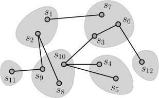
Figure 5.6: The solid edges denote the pairs ${{\cal P}^{(i)}}$, and the grey regions denote the equivalence classes. Let $\smash{{\cal P}_{X}^{(i)}}$ be the pairs $\{(S_{2},S_{9}),(S_{4},S_{10}),(S_{3},S_{10}),(S_{3},S_{6})\}$. Assume that leaders of $S_{11}$ and $S_{12}$ belong to ${\mathscr{D}}_{2}$ (the leaders of the rest of the supernodes must be in ${\mathscr{D}}_{1}$ because the equivalence classes corresponding to these supernodes have cardinality larger than 1). So, ${{\cal P}_{G}^{(i)}}$ consists of pairs $\{(S_{6},S_{12}),(S_{11},S_{9})\}$ and $\smash{{\cal P}_{B}^{(i)}}$ consists of $\{(S_{1},S_{7}),(S_{2},S_{8}),(S_{5},S_{10})\}$.

This completes the construction of the set $\smash{F_{2}^{(i)}}$. The forest $F_{2}$ is obtained by taking the union of $\cup_{i}\smash{F_{2}^{(i)}}$. The task now is to show (a) feasibility, that the edges in $F_{2}$ form a Steiner forest connecting up the demands of ${\mathscr{D}}_{2}$ in metric ${\mathcal{M}}_{1}$, or equivalently that $F_{1}\cup F_{2}$ is a Steiner forest on the set ${\mathscr{D}}_{1}\cup{\mathscr{D}}_{2}$, and (b) strictness, that the cost of $F_{2}$ is comparable to the cost shares assigned to the demands in ${\mathscr{D}}_{2}$.

Feasibility

First, we show feasibility, i.e., that $F_{1}\cup F_{2}$ connects all pairs in ${\mathscr{D}}_{2}$. Observe that we took the run ${\mathcal{R}}$, and added to $F_{2}$ some of the edges added in ${\mathcal{R}}$. Had we added all the edges, we would trivially get feasibility (but not the strictness), but we omitted edges corresponding to pairs in $\smash{{\cal P}_{X}^{(i)}}$. The idea of the proof is that such supernodes will get connected due to the other connections, and to the fact that we inflated the activity times in the TimedPD algorithm. Let’s give the formal proof, which proceeds by induction over time.

For integer $i$, define $\smash{F_{1}^{(\leq i)}}:=\cup_{j\leq i}\smash{F_{1}^{(j)}}$, and define $\smash{F_{2}^{(\leq i)}}$ similarly. The first claim relates the stages in the run ${\mathcal{R}}$ of TimedGlut $({\mathscr{D}}_{1}\cup{\mathscr{D}}_{2})$ to the stages in the run of TimedPD.

Claim 5.11

If terminal $s\in{\mathscr{D}}_{1}$ is active at the beginning of stage $i$ in the run ${\mathcal{R}}$, then the moat containing $s$ remains active during stage $i$ of the run of TimedPD on ${\mathscr{D}}_{1}$.

Proof.

Since $s\in{\mathscr{D}}_{1}$ is active in stage $i$, $\mathsf{level}(s)\geq i$. Hence its activity time $\mathsf{time}(s)\geq 4\cdot 2^{i+1}$. Since stage $i$ for the timed primal-dual algorithm ends at time $4\cdot 2^{i+1}$, the moat containing $s$ in TimedPD will be active at least until the end of stage $i$. ∎

Lemma 5.12

Let ${{\mathscr{C}}}^{i}$ be the clustering at the beginning of stage $i$ in the run ${\mathcal{R}}$. Then,

• For any $S\in{{\mathscr{C}}}^{i}$, all terminals in $S$ lie in the same connected component of $\smash{F_{1}^{(\leq i-1)}}\cup\smash{F_{2}^{(\leq i-1)}}$.

• For every $(S,S^{\prime})\in{{\cal P}^{(i)}}\setminus\smash{{\cal P}_{X}^{(i)}}$, the terminals in $S\cup S^{\prime}$ lie in the same connected component of $\smash{F_{1}^{(\leq i-1)}}\cup\smash{F_{2}^{(\leq i)}}$.

Proof.

We first show that if the statement (a) is true for some stage $i$, then the corresponding statement (b) is also true (for this stage). Consider a pair $(S,S^{\prime})\in{{\cal P}^{(i)}}$. If $(S,S^{\prime})\in{{\cal P}_{G}^{(i)}}\cup\smash{{\cal P}_{B}^{(i)}}$, the edges we add to $\smash{F_{2}^{(i)}}$ would connect the terminals in $S\cup S$, as long as all the supernodes in ${{\mathscr{C}}}^{i}$ formed connected components. But by the assumption, we know that edges in $\smash{F_{1}^{(\leq i-1)}}\cup\smash{F_{2}^{(\leq i-1)}}$ connect up each supernode in ${{\mathscr{C}}}^{i}$. Consequently, terminals in $S\cup S^{\prime}$ lie in the same connected component of $\smash{F_{1}^{(\leq i-1)}}\cup\smash{F_{2}^{(\leq i)}}$. This proves statement (b).

We now prove statement (a) by induction on $i$. At the beginning of stage $i=0$, each supernode $S$ is a singleton and hence the statement is true.

Now to prove the induction step for (a). It suffices to show that if $(S,S^{\prime})\in\smash{{\cal P}_{X}^{(i)}}$ then $S\cup S^{\prime}$ is contained in the same component in $\smash{F_{1}^{(\leq i)}}\cup\smash{F_{2}^{(\leq i)}}$. We distinguish two cases. The first case is when $S$ and $S^{\prime}$ both lie in the same equivalence class that was used to construct $\smash{{\cal P}_{X}^{(i)}}$. Then $s=\mathsf{leader}(S)$ and $s^{\prime}=\mathsf{leader}(S^{\prime})$ belong to ${\mathscr{D}}_{1}$ and also to the same moat in ${\mathfrak{M}_{1}^{(i+1)}}$, at the end of stage $i$. Since $S,S^{\prime}$ are active in stage $i$ of TimedGlut (${\mathscr{D}}$), both $s,s^{\prime}$ have level at least $i$. By Claim 5.11 they remain active throughout stage $i$ of TimedPD. Moreover, the end of that stage they share the same moat. Hence, $s,s^{\prime}$ belong to the same moat when active—but recall that the TimedPD algorithm ensures that whenever two active terminals belong to the same moat they lie in the same connected component. Hence $s,s^{\prime}$ must lie in the same connected component of $\smash{F_{1}^{(\leq i)}}$. By the induction hypothesis, the rest of $S,S^{\prime}$ are connected to their leaders in $\smash{F_{1}^{(\leq i-1)}}\cup\smash{F_{2}^{(\leq i-1)}}$. Hence $S,S^{\prime}$ are connected in $\smash{F_{1}^{(\leq i)}}\cup\smash{F_{2}^{(\leq i-1)}}$; indeed for each equivalence class, the supernodes that belong to it are connected using those edges.

The second case is when for pair $(S,S^{\prime})\in\smash{{\cal P}_{X}^{(i)}}$, the supernodes $S$ and $S^{\prime}$ do not fall in the same equivalence class, but the adding pair $(S,S^{\prime})$ to ${{\cal P}^{(i)}}\setminus\smash{{\cal P}_{X}^{(i)}}$ would form a cycle when equivalence classes are collapsed. The argument here is similar: if the leaders are again $s,s^{\prime}$, then the above arguments applied to each pair on the cycle, and to each equivalence class imply that $s$ and $s^{\prime}$ must be connected in $\smash{F_{1}^{(\leq i)}}\cup\smash{F_{2}^{(\leq i-1)}}$—and therefore so must $S\cup S^{\prime}$. ∎

Since each pair $\{s,\bar{s}\}\in{\mathscr{D}}_{2}$ is contained in some supernode at the end of the run ${\mathcal{R}}$, Lemma 5.12 implies that they are eventually connected in using $F_{1}\cup F_{2}$ as well. This completes the proof that $F_{1}\cup F_{2}$ is a feasible solution to the demands in ${\mathscr{D}}_{2}$.

Bounding the Cost of Forest $F_{2}$

Finally, we want to bound the cost of the edges in $F_{2}$ by a constant times $\sum_{(s,\bar{s})\in{\mathscr{D}}_{2}}\chi({\mathcal{M}},{\mathscr{D}}_{1}\cup{\mathscr{D}}_{2},(s,\bar{s}))$. If $\smash{p_{B}^{(i)}}:=|\smash{{\cal P}_{B}^{(i)}}|$, then the total cost of bad edges is at most

$$\sum_{i}\smash{p_{B}^{(i)}}\cdot 2^{i+1}$$ (5.8)

because the length of edges added for each connection in $\smash{{\cal P}_{B}^{(i)}}$ is at most $2^{i+1}$.

Lemma 5.13

The total cost of the edges in $\cup_{i}\smash{F_{2}^{(i)}}$ is at least $3\sum_{i}\smash{p_{B}^{(i)}}\cdot(2^{i+1}-2^{i})$.

Proof.

For this proof, recall that we run the primal-dual process on the metric ${\mathcal{M}}$, and ${\mathfrak{M}_{1}^{(i)}}$ are the dual moats at the beginning of stage $i$. Let $E_{i}$ denote the set of tight edges lying inside the moats in ${\mathfrak{M}_{1}^{(i)}}$. We prove the following statement by induction on $i$: the total cost of edges in $\smash{F_{2}^{(\leq i)}}\cap E_{i}$ is at least $3\sum_{j\leq i}\smash{p_{B}^{(j)}}\cdot(2^{j+1}-2^{j})$.

The base case for $i=0$ follows trivially because the $\smash{F_{2}^{(0)}}$ is empty, and $\smash{p_{B}^{(0)}}$ is also 0.

Suppose the statement is true for some $i-1$. Now consider the pairs in $\smash{{\cal P}_{B}^{(i)}}$—these correspond to pairs of supernodes $(S,S^{\prime})$ whose leaders lie in ${\mathscr{D}}_{1}$. The pairs in $\smash{{\cal P}_{B}^{(i)}}$ form an acyclic set in the auxiliary graph ${H^{(i)}}$. Consider the set of supernodes which occur as endpoints of the edges in $\smash{{\cal P}_{B}^{(i)}}$, and let $L_{B}$ be the set of terminals that are the leaders of these supernodes. Now pick a maximal set of these supernodes subject to the constraint that all of them lie in different moats in ${\mathfrak{M}_{1}^{(i+1)}}$; i.e., no two of them lie in the same equivalence class. Let $L^{\star}_{B}\subseteq L_{B}$ be the set of terminals that are leaders of this maximal set. In the example given in Figure 5.6, $L_{B}=\{S_{1},S_{2},S_{5},S_{7},S_{8},S_{10}\}$, and we could define $L^{\star}_{B}$ as $\{S_{1},S_{5},S_{7},S_{8}\}$. By the fact that $\smash{{\cal P}_{B}^{(i)}}$ is an acyclic set, we get $|L^{\star}_{B}|\geq\smash{p_{B}^{(i)}}+1$.

For any $s\in L_{B}$, let $M_{s}$ be the moat in ${\mathfrak{M}_{1}^{(i)}}$ containing $s$. By construction,

• For each pair $(S,S^{\prime})\in\smash{{\cal P}_{B}^{(i)}}$, the leaders of $S$ and $S^{\prime}$ lie in different moats in ${\mathfrak{M}_{1}^{(i+1)}}$.

• For all $s\neq s^{\prime}\in L_{B}^{\star}$, $s$ and $s^{\prime}$ belong to different moats in ${\mathfrak{M}_{1}^{(i+1)}}$.

Also note that terminals in distinct moats of ${\mathfrak{M}_{1}^{(i+1)}}$ a fortiori lie in distinct moats in ${\mathfrak{M}_{1}^{(i)}}$. Now contract all the moats in ${\mathfrak{M}_{1}^{(i)}}$ in the metric ${\mathcal{M}}$. Observe that all edges in $\smash{F_{1}^{(\leq i-1)}}$ were already tight by the end of stage $i-1$, and hence get contracted by this operation.

By Lemma 5.12(b), for each $s\in L_{B}^{\star}$ the edges in $\smash{F_{1}^{(\leq i-1)}}\cup\smash{F_{2}^{(\leq i)}}$ connect moat $M_{s}$ to some another moat $M_{s^{\prime}}$ for some $s^{\prime}\in L_{B}$ (corresponding to the pair in $\smash{{\cal P}_{B}^{(i)}}$). Since we contracted the moats in ${\mathfrak{M}_{1}^{(i)}}$, the edges in $\smash{F_{2}^{(\leq i)}}$ connect $M_{s}$ to $M_{s^{\prime}}$ in this contracted metric. But any two moats $M_{s},M_{s^{\prime}}$ are at least $6\cdot(2^{i+1}-2^{i})$ apart in this contracted metric (because these moats do not meet during stage $i$ of the primal dual growing process, else $s,s^{\prime}$ would share a moat in ${\mathfrak{M}_{1}^{(i+1)}}$). Therefore, if we draw a ball of radius $3(2^{i+1}-2^{i})$ around the moat $M_{s}$ in this contracted metric, this ball contains edges from $\smash{F_{2}^{(\leq i)}}$ of length at least $3(2^{i+1}-2^{i})$.

Since these balls around the terminals in $L_{B}^{\star}$ are all disjoint, the total length of all edges in these balls is at least

$$|L_{B}^{\star}|\cdot 3\cdot(2^{i+1}-2^{i})\geq 3(\smash{p_{B}^{(i)}}+1)\cdot(2^{i+1}-2^{i}).$$

All these edges lie in moats in ${\mathfrak{M}_{1}^{(i+1)}}$ but not within moats in ${\mathfrak{M}_{1}^{(i)}}$, so we add these to the bound we get for $\smash{F_{2}^{(\leq i-1)}}\cap E_{i-1}$ from the induction hypothesis and complete the inductive step. ∎

Theorem 5.14

The cost of edges in $F_{2}$ is at most $6\gamma_{{\scriptscriptstyle TG}}$ times $\sum_{(s,\bar{s})\in{\mathscr{D}}_{2}}\chi({\mathcal{M}},{\mathscr{D}}_{1}\cup{\mathscr{D}}_{2},(s,\bar{s}))$.

Proof.

By Lemma 5.13, the cost of edges in $F_{2}$ is at least $3\sum_{i}\smash{p_{B}^{(i)}}\cdot(2^{i+1}-2^{i})\geq\frac{3}{2}\sum_{i}\smash{p_{B}^{(i)}}\cdot 2^{i+1}$. Out of these, the bad edges have total cost at most $\sum_{i}\smash{p_{B}^{(i)}}\cdot 2^{i+1}$, by (5.8). So the cost of the good edges in $F_{2}$ is at least one third of the cost of all edges in $F_{2}$.

However, observe that good edges correspond to pairs $(S,S^{\prime})\in{{\cal P}_{G}^{(i)}}$ for some $i$, i.e., this pair of supernodes was connected by these good edges in stage $i$ of TimedGlut, and moreover, at least one of the leaders of $S$ and $S^{\prime}$ belong to a terminal pair in ${\mathscr{D}}_{2}$. By the construction of our cost shares, it follows the cost share of terminal pairs in ${\mathscr{D}}_{2}$ is at least $\frac{1}{2\gamma_{{\scriptscriptstyle TG}}}$ times the cost of the good edges. Hence the cost of the forest $F_{2}$ is at most $6\gamma_{{\scriptscriptstyle TG}}$ times the cost share of terminal pairs in ${\mathscr{D}}_{2}$, proving the theorem. ∎

Acknowledgments

We thank R. Ravi for suggesting the problem to us, for many discussions about it over the years, and for the algorithm name. We also thank Chandra Chekuri, Jochen Könemann, Stefano Leonardi, and Tim Roughgarden.

Appendix A The Lower Bound for (Paired) Greedy

The (paired) greedy algorithm picks, at each time the closest yet-unconnected source-sink pair $(s,\bar{s})$ in the current graph, and connects them using a shortest $s$-$\bar{s}$ path in the current graph. A lower bound of $\Omega(\log n)$ for this algorithm was given by Chen, Roughgarden, and Valiant [CRV10]. We repeat this lower bound here for completeness.

Take a cubic graph $G=(V,E)$ with $n$ nodes and girth at least $c\log n$ for constant $c$; see [Big98] for constructions of such graphs. Fix a spanning tree $T$ of $G$, and let $E^{\prime}=E\setminus E(T)$ be the non-tree edges. Set the lengths of edges in $E(T)$ to $1$, and the lengths of edges in $E^{\prime}$ to $\frac{c}{2}\log n$.

Let $M$ be a maximal matching in $G^{\prime}=(V,E^{\prime})$; since $G$ and hence $G^{\prime}$ has maximum degree $3$, this maximal matching has size at least $\Omega(|E^{\prime}|)=\Omega(n)$. The demand set ${\mathscr{D}}$ consists of the matching $M$.

We claim that the paired-greedy algorithm will just buy the direct edges connecting the demand pairs. This will incur cost $|M|\cdot\frac{c}{2}\log n=\Omega(n\log n)$. The optimal solution, on the other hand, is to buy the edges of $T$, which have total cost $n-1$, which gives the claimed lower bound of $\Omega(\log n)$.

The proof of the claim about the behavior of paired-greedy is by induction. Suppose it is true until some point, and then demand $(u,v)$ is considered. By construction, $(u,v)\in M$. We can model the fact that we bought some previous edges by zeroing out their lengths. Now the observation is that for any path $P$ between $u$ and $v$ that is not the direct edge $(u,v)$, if there are $k$ edges from $E^{\prime}$ on this path, then at most $\lceil k/2\rceil$ of them can be zeroed out. Moreover, since the girth is $g$, the number of edges on the path is at least $g-1$. So the new length of the path $P$ is at least $(g-1-k)+\lfloor k/2\rfloor\frac{c}{2}\log n\geq g-2$. This means the direct edge between $u,v$ is still the (unique) shortest path, and this proves the claim and the result.

Appendix B A Different Gluttonous Algorithm, and its Analysis

In this section, we consider a slightly different analysis of the gluttonous algorithm which does not rely on the faithfulness property developed in Section 3.2. We then use this analysis to show that a different gluttonous algorithm is also a constant-factor approximation.

As before, let $\mathscr{F}^{\star}$ denote an optimal solution to the Steiner forest instance ${\mathscr{I}}=({\mathcal{M}},{\mathscr{D}})$, and let the trees in $\mathscr{F}^{\star}$ be $T^{\star}_{1},T^{\star}_{2},\ldots,T^{\star}_{p}$. A supernode $S$ is a subset of terminals – note that we no longer require that the supernodes formed during the gluttonous algorithm should be contained in one of the trees of $\mathscr{F}^{\star}$. Let ${{\mathscr{C}}}^{(t)}$ denote the clustering at the beginning of iteration $t$. So ${{\mathscr{C}}}^{(1)}$ consists of singleton supernodes.

For each index $r$, $1\leq r\leq p$, we can think of a new instance ${\mathscr{I}}_{r}$ with set of terminals $V(T^{\star}_{r})$ and metric ${\mathcal{M}}_{r}$ (the metric ${\mathcal{M}}$ restricted to these terminals). We now define the notion of projected supernodes. For each tree $T^{\star}_{r}$, we shall maintain a clustering ${{\mathscr{C}}}^{(t)}_{r}$ corresponding to ${{\mathscr{C}}}^{(t)}$ – this should be seen as the restriction of the algorithm ${\mathscr{A}}$ to the instance ${\mathscr{I}}_{t}$. A natural way of defining this would be $S\cap V(T^{\star}_{r})$ for every $S\in{{\mathscr{C}}}^{(t)}$. But it turns out that we will really need a refinement of the latter clustering. The reason for this is as follows: if the algorithm ${\mathscr{A}}$ merges two active supernodes in the instance ${\mathscr{I}}$, the intersection of the two supernodes with $V(T^{\star}_{r})$ may be inactive supernodes. But we do not want to combine two inactive supernodes in the clustering ${{\mathscr{C}}}^{(t)}_{r}$.

We now define the clustering ${{\mathscr{C}}}^{(t)}_{r}$ formally. For a supernode $S$, let $S_{r}$ denote $S\cap V(T^{\star}_{r})$. We say that $S_{r}$ is active if there is some demand pair $(u,{\bar{u}})$ such that $u\in S_{r}$, but ${\bar{u}}\notin S_{r}$. Let $\mathsf{alive}(S)$ denote the set of indices $r$ such that $S_{r}$ is active. For each iteration $t$, we shall maintain the following invariants.

• The clustering ${{\mathscr{C}}}^{(t)}_{r}$ will be a refinement of the clustering $\{S_{r}:S\in{{\mathscr{C}}}^{(t)}\}$.

• For each (active) supernode $S\in{{\mathscr{C}}}^{(t)}$ such that $S_{r}$ is active, there will be exactly one active supernode ${\mathsf{A}}_{r}(S)\subseteq S_{r}$ in the clustering ${{\mathscr{C}}}^{(t)}_{r}$.

Initially, ${{\mathscr{C}}}^{(1)}_{r}$ is the clustering consisting of singleton sets (it is easy to check that it satisfies the two invariants above because ${{\mathscr{C}}}^{(1)}$ also consists of singleton sets). Suppose at iteration $t$, the algorithm ${\mathscr{A}}$ merges supernodes $S^{\prime}$ and $S^{\prime\prime}$ to a supernode $S$. If $S^{\prime}_{r}$ and $S^{\prime\prime}_{r}$ are both active (i.e., $r\in\mathsf{alive}(S^{\prime})\cap\mathsf{alive}(S^{\prime\prime})$), then we replace ${\mathsf{A}}_{r}(S^{\prime})$ and ${\mathsf{A}}_{r}(S^{\prime\prime})$ by their union in the clustering ${{\mathscr{C}}}^{(t)}_{r}$ to get ${{\mathscr{C}}}^{(t+1)}_{r}$. Otherwise, ${{\mathscr{C}}}^{(t+1)}_{r}$ is same as ${{\mathscr{C}}}^{(t)}_{r}$. It is easy to check that the above two invariants will still be satisfied. Further, observe that we only merge two active supernodes of ${{\mathscr{C}}}^{(t)}_{r}$, and an inactive supernode never merges with any other supernode.

Let $\delta_{t,r}$ denote the minimum over two active supernodes $S^{\prime},S^{\prime\prime}\in{{\mathscr{C}}}^{(t)}_{r}$ of $d_{{\mathcal{M}}_{r}/{{\mathscr{C}}}^{(t)}_{r}}(S^{\prime},S^{\prime\prime})$ (in case ${{\mathscr{C}}}^{(t)}_{r}$ has only one active supernode, this quantity is infinity). Fact 3.12 implies that $\delta_{t,r}$ is ascending with $t$. Let $\delta_{t}$ denote the minimum over all $r$ of $\delta_{t,r}$. Clearly, $\delta_{t}$ is also ascending with $t$.

Whenever the algorithm merges active supernodes $S^{\prime}$ and $S^{\prime\prime}$, we will think of merging the corresponding supernodes ${\mathsf{A}}_{r}(S^{\prime})$ and ${\mathsf{A}}_{r}(S^{\prime\prime})$ in the instance ${\mathscr{I}}_{r}$ for each value of $r$ (provided $r\in\mathsf{alive}(S^{\prime})\cap\mathsf{alive}(S^{\prime\prime})$). Note that the latter merging cost may not suffice to account for the merging cost of $S^{\prime}$ and $S^{\prime\prime}$. For example, suppose $S^{\prime}=\{a\},S^{\prime\prime}=\{b\}$, and $a$ and $b$ happen to be in different trees in $\mathscr{F}^{\star}$, say $T^{\star}_{1}$ and $T^{\star}_{2}$ respectively. If $S=\{a,b\}$ is the new supernode, then ${\mathsf{A}}_{1}(S)={\mathsf{A}}_{1}(S^{\prime})=\{a\}$ and ${\mathsf{A}}_{2}(S)={\mathsf{A}}_{2}(S^{\prime\prime})=\{b\}$. So the merging costs in the corresponding instances is 0, but the actual merging cost is positive. The main idea behind the proof is that we will pay for this merging cost later when the algorithm merges the supernode containing $a$ with some other supernode which has non-empty intersection with $T^{\star}_{1}$ (and similarly for $b$).

In order to keep track of the unpaid merging cost, we associate a charge with each supernode (which gets formed during the gluttonous algorithm ${\mathscr{A}}$) – let $\mathsf{charge}(S)$ denote this quantity. At the beginning of every every iteration $t$ and supernode $S\in{{\mathscr{C}}}^{(t)}$, we will maintain the following invariant:

$$\mathsf{charge}(S)\leq\left\{\begin{array}[]{ll}0&\mbox{if $S$ is inactive at the beginning of iteration $t$. }\\ (n(S)-1)\cdot\delta_{t}&\mbox{ otherwise,}\end{array}\right.$$ (B.11)

where $n(S)$ denotes the number of indices $r$ such that $S_{r}$ is active, i.e., $n(S)=|\mathsf{alive}(S)|$. Now, we show how the quantity $\mathsf{charge}(S)$ is updated. Initially (at the beginning of iteration 1), we have a supernode $\{u\}$ for each terminal $u$. The charge associated with each of these supernodes is 0. Clearly, the invariant condition above is satisfied.

Suppose the algorithm ${\mathscr{A}}$ merges supernodes $S^{\prime}$ and $S^{\prime\prime}$ in iteration $t$. Let $S$ denote the new supernode. We define $\mathsf{charge}(S)$ as

$$\mathsf{charge}(S)=\mathsf{charge}(S^{\prime})+\mathsf{charge}(S^{\prime\prime})-(2|\mathsf{alive}(S^{\prime})\cap\mathsf{alive}(S^{\prime\prime})|-1)\delta_{t}.$$ (B.12)

We first prove that the invariant about charge of a supernode is satisfied.

Claim B.1

The invariant conditions (B.11) are always satisfied.

Proof.

We prove this by induction on the iteration $t$. Suppose ${\mathscr{A}}$ merges (active) supernodes $S^{\prime}$ and $S^{\prime\prime}$ iteration $t$, and let $S$ be the new supernode. If we consider a supernode $S_{1}$ other than $S$ in ${{\mathscr{C}}}^{(t+1)}$, then the statement follows easily. Note that $\mathsf{charge}(S_{1})$ does not change. If $S_{1}$ were inactive before iteration $t$, it will continue to be inactive at the end of iteration $t$ as well. If $S_{1}$ were active before iteration $t$, then it will continue to be active be at the beginning of iteration $(t+1)$ as well. Further, $n(S_{1})$ will not change (and is at least 1), and $\delta_{t+1}\geq\delta_{t}$. So, we now consider the case for $S$ only. We get

$$\mathsf{charge}(S) =\mathsf{charge}(S^{\prime})+\mathsf{charge}(S^{\prime\prime})-(2|\mathsf{alive}(S^{\prime})\cap\mathsf{alive}(S^{\prime\prime})|-1)\delta_{t}$$

$$\leq(n(S^{\prime})-1)\cdot\delta_{t}+(n(S^{\prime\prime})-1)\cdot\delta_{t}-(2|\mathsf{alive}(S^{\prime})\cap\mathsf{alive}(S^{\prime\prime})|-1)\delta_{t}$$

$$\leq(n(S)-1)\cdot\delta_{t},$$

where the last inequality follows from the fact that $n(S)\geq n(S^{\prime})+n(S^{\prime\prime})-2|\mathsf{alive}(S^{\prime})\cap\mathsf{alive}(S^{\prime\prime})|$. Note that it is possible that $r\in\mathsf{alive}(S^{\prime})\cap\mathsf{alive}(S^{\prime\prime})$, but $r\notin\mathsf{alive}(S)$. However, $\mathsf{alive}(S^{\prime})\backslash\mathsf{alive}(S^{\prime\prime}),$ $\mathsf{alive}(S^{\prime\prime})\backslash\mathsf{alive}(S^{\prime})\subseteq\mathsf{alive}(S).$ Finally, observe that if $S$ is active, then $n(S)\geq 1$. This implies that $(n(S)-1)\cdot\delta_{t}\leq(n(S)-1)\cdot\delta_{t+1}$. Therefore, the invariant holds in this case. If $S$ becomes inactive, then $n(S)=0$, and so, $(n(S)-1)\cdot\delta_{t}\leq 0$. Again, the invariant continues to hold here. ∎

When the algorithm starts, $n(S)=1$ for all supernodes $S$ (consisting of singleton terminals). So, $\mathsf{charge}(S)=0$ for all $S$ at time $1$. When the algorithm terminates, $\mathsf{charge}(S)\leq 0$ for all supernodes (since they are inactive). Therefore, adding the inequality (eq:charge) over all iterations $t$, we get

$$\sum_{t}\delta_{t}\leq 2\delta_{t}\cdot\sum_{t}|\mathsf{alive}(S^{\prime})\cap\mathsf{alive}(S^{\prime\prime})|\leq 2\sum_{t}\sum_{r}{\bf 1}[r,t]\cdot\delta_{t,r},$$ (B.13)

where ${\bf 1}[r,t]$ is the indicator variable which is 1 if and only if $r\in\mathsf{alive}(S^{\prime})\cap\mathsf{alive}(S^{\prime\prime})$. The following claim follows easily.

Claim B.2

The merging cost of ${\mathscr{A}}$ in iteration $t$ is at most $\delta_{t}$.

Proof.

Suppose $\delta_{t}=\delta_{t,r}=d_{{\mathcal{M}}_{r}/{{\mathscr{C}}}^{(t)}_{r}}({\mathsf{A}}_{r}(S^{\prime}),{\mathsf{A}}_{r}(S^{\prime\prime}))$ for some active supernodes $S^{\prime},S^{\prime\prime}\in{{\mathscr{C}}}^{(t)}$. Observe that $d_{{\mathcal{M}}/{{\mathscr{C}}}^{(t)}}(S^{\prime},S^{\prime\prime}))\leq d_{{\mathcal{M}}_{r}/{{\mathscr{C}}}^{(t)}_{r}}({\mathsf{A}}_{r}(S^{\prime}),{\mathsf{A}}_{r}(S^{\prime\prime}))$. ∎

Finally, Corollary 3.13 applied to the instance ${\mathscr{I}}_{r}$ shows that

$$\sum_{t}{\bf 1}[r,t]\cdot\delta_{t,r}\leq 48\cdot\mathsf{cost}(T^{\star}_{r}).$$

Combining the above with Claim B.2 and inequality (B.13), we get

Lemma B.3

The total merging cost of the gluttonous algorithm is at most $96$ times that of the optimal solution.

B.1 A Different Gluttonous Algorithm

We apply the above result to analyze a slightly different version of the gluttonous algorithm. As before, the algorithm will maintain a set of supernodes, denoted by ${{\mathscr{C}}}^{(t)}$, at the beginning of iteration $t$. Further, it will maintain an edge-weighted graph ${G^{(t)}}$ with vertex set being ${{\mathscr{C}}}^{(t)}$. Initially, at time $t=1$, ${G^{(1)}}$ is just the initial graph $G$ on the vertices (i.e., terminals and Steiner nodes). In iteration $t$, the algorithm picks the two active supernodes with smallest distance between them, where distances are measured with respect to the edge lengths in ${G^{(t)}}$. Let $P_{t}$ be the corresponding shortest path (all internal vertices of $P_{t}$ must be inactive supernodes). We contract all the edges of $P_{t}$ to get the graph ${G^{(t+1)}}$. The clustering ${{\mathscr{C}}}^{(t+1)}$ will be be same as ${{\mathscr{C}}}^{(t)}$ except for the fact that the supernodes corresponding to vertices of $P_{t}$ will get replaced by a new supernode which will be the union of all these supernodes.

For the above algorithm, the proof of Theorem 3.6 does not hold. More specifically, consider case I in the proof where $u$ and $v$ happen to be in the same tree in $\mathscr{F}^{\star\star}$. Now, the algorithm may contract a path with end-points containing $u$ and $v$ respectively. Further, the internal vertices of this path could correspond to inactive supernodes, and so, the new supernode will contain terminals outside this tree. But we cannot pay for the cost of this path. However, we claim that the analysis of this section still applies.

Lemma B.4

The above algorithm is a 96-approximation algorithm for the Steiner forest problem.

Proof.

Let ${\mathscr{B}}$ denote the version of the gluttonous algorithm described above. It is no longer true that an inactive supernode does not merge with any other supernode. In each iteration, the algorithm may choose to merge two active supernodes along with several inactive supernodes. However, the clusterings ${{\mathscr{C}}}^{(t)}_{r}$ will respect the former property.

The clusterings ${{\mathscr{C}}}^{(t)}_{r}$ will respect the invariants (i) and (ii) described above. When the algorithm ${\mathscr{B}}$ merges active supernodes $S^{\prime}$ and $S^{\prime\prime}$ (along with possibly other inactive supernodes), and the index $r\in\mathsf{alive}(S^{\prime})\cap\mathsf{alive}(S^{\prime\prime})$, we merge ${\mathsf{A}}_{r}(S^{\prime})$ and ${\mathsf{A}}_{r}(S^{\prime\prime})$ in the clustering ${{\mathscr{C}}}^{(t)}_{r}$ to get ${{\mathscr{C}}}^{(t+1)}_{r}$. It is easy to check that these two invariants are satisfied. The rest of the proof proceeds without any change. The key property that holds for this algorithm as well is that the merging cost (i.e., length of the shortest path) in each iteration is at most $\delta_{t}$ (defined in the proof above). ∎

References

- [AKR95] Ajit Agrawal, Philip Klein, and R. Ravi. When trees collide: an approximation algorithm for the generalized Steiner problem on networks. SIAM J. Comput., 24(3):440–456, 1995.
- [BGRS13] Jarosław Byrka, Fabrizio Grandoni, Thomas Rothvoss, and Laura Sanità. Steiner tree approximation via iterative randomized rounding. J. ACM, 60(1):Art. 6, 33, 2013.
- [Big98] Norman Biggs. Constructions for cubic graphs with large girth. Electron. J. Combin., 5:Article 1, 25 pp. (electronic), 1998.
- [CRV10] Ho-Lin Chen, Tim Roughgarden, and Gregory Valiant. Designing network protocols for good equilibria. SIAM J. Comput., 39(5):1799–1832, 2010.
- [CS09] Chandra Chekuri and F. Bruce Shepherd. Approximate integer decompositions for undirected network design problems. SIAM J. Discrete Math., 23(1):163–177, 2008/09.
- [FKLS10] Lisa Fleischer, Jochen Könemann, Stefano Leonardi, and Guido Schäfer. Strict cost sharing schemes for Steiner forest. SIAM J. Comput., 39(8):3616–3632, 2010.
- [GGLS08] Naveen Garg, Anupam Gupta, Stefano Leonardi, and Piotr Sankowski. Stochastic analyses for online combinatorial optimization problems. In SODA, pages 942–951, 2008.
- [GK09] Anupam Gupta and Amit Kumar. A constant-factor approximation for stochastic steiner forest. In STOC, pages 659–668, New York, NY, USA, 2009. ACM.
- [GKPR07] Anupam Gupta, Amit Kumar, Martin Pál, and Tim Roughgarden. Approximation via cost sharing: simpler and better approximation algorithms for network design. J. ACM, 54(3):Art. 11, 38 pp., 2007.
- [GPRS11] Anupam Gupta, Martin Pál, R. Ravi, and Amitabh Sinha. Sampling and cost-sharing: approximation algorithms for stochastic optimization problems. SIAM J. Comput., 40(5):1361–1401, 2011.
- [GW95] Michel X. Goemans and David P. Williamson. A general approximation technique for constrained forest problems. SIAM J. Comput., 24(2):296–317, 1995.
- [IKMM04] Nicole Immorlica, David Karger, Maria Minkoff, and Vahab Mirrokni. On the costs and benefits of procrastination: Approximation algorithms for stochastic combinatorial optimization problems. In SODA, pages 684–693, 2004.
- [Jai01] Kamal Jain. A factor 2 approximation algorithm for the generalized Steiner network problem. Combinatorica, 21(1):39–60, 2001. (Preliminary version in 39th FOCS, pages 448–457, 1998).
- [KLS05] Jochen Könemann, Stefano Leonardi, and Guido Schäfer. A group-strategyproof mechanism for steiner forests. In SODA, pages 612–619, 2005.
- [KLSvZ08] Jochen Könemann, Stefano Leonardi, Guido Schäfer, and Stefan H. M. van Zwam. A group-strategyproof cost sharing mechanism for the steiner forest game. SIAM J. Comput., 37(5):1319–1341, 2008.
- [Pál04] M. Pál. Cost Sharing and Approximation. PhD thesis, Cornell University, 2004.
- [RZ05] Gabriel Robins and Alexander Zelikovsky. Tighter bounds for graph Steiner tree approximation. SIAM J. Discrete Math., 19(1):122–134, 2005.