Dynamics of the monodromies of the fibrations on the magic $3$-manifold

Abstract.

We study the magic manifold $N$ which is a hyperbolic and fibered $3$-manifold. We give an explicit construction of a fiber $F_{a}$ and its monodromy $:F_{a}\rightarrow F_{a}$ of the fibration associated to each fibered class $a$ of $N$. Let $\delta_{g}$ (resp. $\delta_{g}^{+}$) be the minimal dilatation of pseudo-Anosovs (resp. pseudo-Anosovs with orientable invariant foliations) defined on an orientable closed surface of genus $g$. As a consequence of our result, we obtain the first explicit construction of the following pseudo-Anosovs; a minimizer of $\delta_{7}^{+}$ and conjectural minimizers of $\delta_{g}$ for large $g$.

1. Introduction

In this paper, we explore the dynamics of monodromies of fibrations on a hyperbolic, fibered $3$-manifold, called the magic $3$-manifold $N$, which is the exterior of the $3$ chain link $\mathcal{C}_{3}$, see Figure 1(1). We first set some notations, then describe the motivation of our study. Let $\varSigma$ be an orientable surface (possibly with punctures). A homeomorphism $\Phi:\varSigma\rightarrow\varSigma$ is pseudo-Anosov if there exist a pair of transverse measured foliations $(\mathcal{F}^{u},\mu^{u})$ and $(\mathcal{F}^{s},\mu^{s})$ and a constant $\lambda=\lambda(\Phi)>1$ such that

$$\Phi(\mathcal{F}^{u},\mu^{u})=(\mathcal{F}^{u},\lambda\mu^{u})\ \hskip 5.69054pt\mbox{and}\ \hskip 5.69054pt\Phi(\mathcal{F}^{s},\mu^{s})=(\mathcal{F}^{s},\lambda^{-1}\mu^{s}).$$

Then $\mathcal{F}^{u}$ and $\mathcal{F}^{s}$ are called the unstable and stable foliations (or invariant foliations), and $\lambda$ is called the dilatation of $\Phi$. Let $\mathrm{Mod}(\varSigma)$ be the mapping class group of $\varSigma$, that is $\mathrm{Mod}(\varSigma)$ is the group of isotopy classes of orientation preserving homeomorphisms on $\varSigma$ fixing punctures setwise. A mapping class $\phi\in\mathrm{Mod}(\varSigma)$ is called pseudo-Anosov if $\phi$ contains a pseudo-Anosov homeomorphism $\Phi:\varSigma\rightarrow\varSigma$ as a representative. The topological entropy $\mathrm{ent}(\Phi)$ of $\Phi$ is equal to $\log\lambda(\Phi)$, and $\mathrm{ent}(\Phi)$ attains the minimal entropy among all homeomorphisms which are isotopic to $\Phi$, see [5, Exposé 10]. In the case $\phi=[\Phi]$, we denote by $\lambda(\phi)$ and $\mathrm{ent}(\phi)$, the dilatation $\lambda(\Phi)$ and topological entropy $\mathrm{ent(\Phi)}=\log\lambda(\Phi)$.

We take an element $\phi\in\mathrm{Mod}(\varSigma)$. Let ${\mathbb{T}}_{\phi}$ be its mapping torus, i.e, if $\Phi$ is a representative of $\phi$, then

$${\mathbb{T}}_{\phi}=\varSigma\times{\mathbb{R}}/\sim$$

where $\sim$ identifies $(x,t+1)$ with $(\Phi(x),t)$ for $x\in\varSigma$ and $t\in{\mathbb{R}}$. Such a $\Phi$ is called the monodromy of ${\mathbb{T}}_{\phi}$. The vector field $\frac{\partial}{\partial t}$ on $\varSigma\times{\mathbb{R}}$ induces a flow $\Phi^{t}$ on ${\mathbb{T}}_{\phi}$, which is called the suspension flow. The hyperbolization theorem by Thurston [36] tells us that a $3$-manifold $M$ which is homeomorphic to ${\mathbb{T}}_{\phi}$ admits a hyperbolic structure if and only if $\phi$ is pseudo-Anosov. The magic manifold $N$ is in fact a hyperbolic, fibered $3$-manifold, since $N$ is homeomorphic to a $4$-puncture sphere bundle over the circle with the pseudo-Anosov monodromy as in Figure 1(2) (see Lemma 2.6(1)).

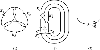
Figure 1. (1) $3$ chain link $\mathcal{C}_{3}$. (2) Braided link $\mathrm{br}(\sigma_{1}^{2}\sigma_{2}^{-1})$. Our convention of the orientation is that the meridian of a component of the link is chosen as in (3).

In a paper [35] Thurston introduced a norm $\|\cdot\|$ on $H_{2}(M,\partial M;{\mathbb{R}})$ for hyperbolic $3$-manifolds and proved that the unit ball $U_{M}$ with respect to the Thurston norm $\|\cdot\|$ is a compact, convex polyhedron. When $M$ is homeomorphic to a hyperbolic, fibered $3$-manifold ${\mathbb{T}}_{\phi}$, he gave a connection between the Thurston norm $\|\cdot\|$ and fibrations on $M$. In particular if such a $3$-manifold $M$ has the second Betti number $b_{2}(M)$ which is greater than $1$, he proved that there exists a top dimensional face $\Omega$ on $\partial U_{M}$, called a fibered face such that every integral class $a$ of $H_{2}(M,\partial M;{\mathbb{Z}})$ which is in the open cone over $\Omega$ corresponds to a fiber $F_{a}$ of the fibration associated to $a$ with a monodromy $\Phi_{a}:F_{a}\rightarrow F_{a}$, that is ${\mathbb{T}}_{\phi_{a}}$ is homeomorphic to $M$, where $\phi_{a}=[\Phi_{a}]$. Such an integral class $a$ is called a fibered class.

Since $\phi_{a}=[\Phi_{a}]$ is pseudo-Anosov for each fibered class $a$, $M$ provides infinitely many pseudo-Anosovs on fibers with distinct topological types. A theorem by Fried [6, 7] asserts that the monodromy $\Phi_{a}:F_{a}\rightarrow F_{a}$ and the (un)stable foliation $\mathcal{F}_{a}$ of $\Phi_{a}$ can be described by using the suspension flow $\Phi^{t}$ and the suspension of the (un)stable foliation of $\Phi$. A question we would like to pose is that how about practical constructions of $\Phi_{a}:F_{a}\rightarrow F_{a}$ and $\mathcal{F}_{a}$ for each fibered class $a$. The theorem by Fried does not give us concrete descriptions of them.

E. Hironaka gave concrete descriptions of the monodorimies of fibrations associated to sequences of fibered classes on some class of hyperbolic fibered $3$-manifolds, see [11, 12]. However no one constructed explicitly the monodromy of the fibration associated to each fibered class on a single hyperbolic, fibered $3$-manifold $M$ with $b_{2}(M)>1$. In this paper we describe them concretely for the magic manifold $N$. The motivation of our study comes from minimal dilatations on pseudo-Anosovs and their asymptotic behaviors. We fix a surface $\varSigma$, and consider the set of dilatations of pseudo-Anosovs on $\varSigma$,

$$\mathrm{dil}(\varSigma)=\{\lambda(\phi)\ |\ \phi\in\mathrm{Mod}(\varSigma)\ \mbox{is pseudo-Anosov}\}.$$

Arnourx-Yoccoz and Ivanov observed that for any constant $c>1$, there exist finite elements $\lambda\in\mathrm{dil}(\varSigma)$ so that $\lambda<c$, see [15]. In particular, there exists a minimum $\delta(\varSigma)$ of $\mathrm{dil}(\varSigma)$. Let $\varSigma_{g}$ be a closed surface of genus $g$, and $\varSigma_{g,n}$ a closed surface of genus $g$ removing $n\geq 1$ punctures. We let $\delta_{g}=\delta(\varSigma_{g})$ and $\delta_{g,n}=\delta(\varSigma_{g,n})$. We denote by $D_{n}$, an $n$-punctured disk. A mapping class $\phi\in\mathrm{Mod}(D_{n})$ defines a mapping class $\phi^{\prime}\in\mathrm{Mod}(\varSigma_{0,n+1})$ fixing a puncture and vice versa. Moreover $\phi$ is pseudo-Anosov if and only if $\phi^{\prime}$ is pseudo-Anosov. In this case the equality $\lambda(\phi)=\lambda(\phi^{\prime})$ holds. Thus $\delta(D_{n})$ is equal to the minimal dilatations among pseudo-Anosov elements $\phi^{\prime}\in\mathrm{Mod}(\varSigma_{0,n+1})$ fixing a puncture. In particular we have $\delta(D_{n})\geq\delta(\varSigma_{0,n+1})$.

The minimal dilatation problem is to determine an explicit value of $\delta(\varSigma)$, and to identify a pseudo-Anosov element $\phi\in\mathrm{Mod}(\varSigma)$ which achieves $\delta(\varSigma)$ (i.e, minimizer of $\delta(\varSigma)$). Naive but natural question is this: What does the pseudo-Anosov homeomorphism $\Phi$ on $\varSigma$ which achieves $\delta(\varSigma)$ look like? In other words, what does a train track representative of $\phi=[\Phi]$ (which enables us to describe the dynamics of $\Phi:\varSigma\rightarrow\varSigma$) look like?

Table 1. Asymptotic behaviors of minimal dilatations and smallest known upper bounds, where $\delta(D_{4})\approx 2.2966$ is the largest root of $t^{4}-2t^{3}-2t+1$ [21], and $\delta(D_{5})\approx 1.7220$ is the largest root of $t^{4}-t^{3}-t^{2}-t+1$ [9].

$\left|\begin{array}[]{c r|c c r}\hline\cr\mbox{asymptotic behaviors}&&&\mbox{smallest known upper bounds}&\\ \hline\cr\log\delta_{g}\asymp 1/g&\mbox{\cite[cite]{[\@@bibref{}{Penner}{}{}]}}&\mbox{(U1)}&\displaystyle\limsup_{g\to\infty}\,g\log\delta_{g}\leq\log(\tfrac{3+\sqrt{5}}{2})&\mbox{\cite[cite]{[\@@bibref{}{Hironaka,AD,KT1}{}{}]}}\\ \hline\cr\log\delta_{g}^{+}\asymp 1/g&\mbox{\cite[cite]{[\@@bibref{}{Minakawa,HK}{}{}]}}&\mbox{(U2)}&\displaystyle\limsup_{\begin{subarray}{c}g\not\equiv 0\pmod{6}\\ g\to\infty\end{subarray}}g\log\delta_{g}^{+}\leq\log(\tfrac{3+\sqrt{5}}{2})&\mbox{\cite[cite]{[\@@bibref{}{Hironaka,KKT2}{}{}]}}\\ &&\mbox{(U3)}&\displaystyle\limsup_{\begin{subarray}{c}g\equiv 6\pmod{12}\\ g\to\infty\end{subarray}}g\log\delta^{+}_{g}\leq 2\log\delta(D_{5})&\mbox{\cite[cite]{[\@@bibref{}{KKT2}{}{}]}}\\ \hline\cr\log\delta_{0,n}\asymp 1/n&\mbox{\cite[cite]{[\@@bibref{}{HK}{}{}]}}&\mbox{(U4)}&\displaystyle\limsup_{n\to\infty}n\log\delta_{0,n}\leq 2\log(2+\sqrt{3})&\mbox{\cite[cite]{[\@@bibref{}{HK,KT}{}{}]}}\\ \hline\cr\log\delta_{1,n}\asymp 1/n&\mbox{\cite[cite]{[\@@bibref{}{Tsai}{}{}]}}&\mbox{(U5)}&\displaystyle\limsup_{n\to\infty}n\log\delta_{1,n}\leq 2\log\delta(D_{4})&\mbox{\cite[cite]{[\@@bibref{}{KKT2}{}{}]}}\\ \hline\cr\mbox{Given}\ g\geq 2,\ \log\delta_{g,n}\asymp\frac{\log n}{n}&\mbox{\cite[cite]{[\@@bibref{}{Tsai}{}{}]}}&\mbox{(U6)}&\displaystyle\limsup_{n\to\infty}\tfrac{n\log\delta_{g,n}}{\log n}\leq 2\ \mbox{if}\ g\ \mbox{enjoys\ }(*)&\mbox{\cite[cite]{[\@@bibref{}{KT2}{}{}]}}\\ \hline\cr\end{array}\right|$

Some of the minimal dilatations are already determined. Also there are partial results. For example, $\delta_{2}$ is computed in [4], but an explicit value of $\delta_{g}$ is not known for $g\geq 3$. If we denote by $\delta_{g}^{+}$, the minimal dilatation of pseudo-Anosovs defined on $\varSigma_{g}$ with orientable invariant foliations, then explicit values of $\delta_{g}^{+}$ for $2\leq g\leq 8$ except $g=6$ are known, see [39, 22] and [10, 1, 19]. The minimal dilatation on an $n$-punctured disk, $\delta(D_{n})$ is determined for $3\leq n\leq 8$, see [21, 9, 23].

The asymptotic behaviors of the minimal dilatations are shown in the left column of Table 1. Here $A_{g}\asymp B_{g}$ means that there exists a constant $c>0$ which does not depend on $g$ so that $\tfrac{A_{g}}{c}<B_{g}<cA_{g}$. As we can see from table, we have $\log\delta_{0,n}\asymp 1/n$ and $\log\delta_{1,n}\asymp 1/n$, but a result by Tsai [37] says that the situation in the case $g\geq 2$ is quite different from the case $g=0$ or $1$. In the right column of Table 1, the smallest known upper bounds of the minimal dilatation. We give a precise condition $(*)$ in (U6) in the following.

Theorem 1.1 ([20]).

Suppose that $g\geq 2$ satisfies

$(*)$    $\gcd(2g+1,s)=1$ or $\gcd(2g+1,s+1)=1$ for each $0\leq s\leq g$.

Then

(1.1) $$\limsup_{n\to\infty}\frac{n\log\delta_{g,n}}{\log n}\leq 2.$$

In particular, if $2g+1$ is prime, then $g$ enjoys $(*)$, and hence (1.1) holds.

The upper bounds (U1)–(U6) are proved by examples of sequences of pseudo-Anosovs. The magic manifold $N$ is involved in these upper bounds. There exists a sequence of fibered classes of $N$ corresponding to each of (U1), $\cdots$, (U6). The projection onto a fibered face of the sequence corresponding to (U6) converges to a single point which lies on the boundary of a fibered face of $N$. On the other hand, the projection of other sequence converges to some point in the interior of the fibered face of $N$. An interesting feature is the following. The mapping torus ${\mathbb{T}}_{\phi}$ of each example $\phi$ which appears in the sequences is either $N$ or the fibration of ${\mathbb{T}}_{\phi}$ comes from a fibration of $N$ by Dehn filling cusps along the boundary slopes of a fiber. This is also true for known minimizers of the minimal dilatations $\delta_{2}$, $\delta(D_{n})$ for $3\leq n\leq 8$ and $\delta_{g}^{+}$ for $2\leq g\leq 8$ except $g=6$. These results say that the topological types of fibers of fibrations on $N$ are surprisingly full of variety. However, no explicit constructions of sequences of pseudo-Anosovs needed for the proofs of (U1)–(U6) except (U4) were given so far. Also an explicit example of a minimizer of $\delta_{7}^{+}$ was not given. In this paper we prove the following which allows us to construct pseudo-Anosovs in question explicitly.

Theorem 1.2.

We have algorithms to construct the followings. For each fibered class $a$ of $N$,

1. the monodromy $\Phi_{a}:F_{a}\rightarrow F_{a}$ of the fibration on $N$ associated to $a$, and

2. in the case $a$ is primitive, a train track representative $\mathfrak{p}_{a}:\tau_{a}\rightarrow\tau_{a}$ of $\phi_{a}=[\Phi_{a}]$ whose incidence matrix is Perron-Frobenius.

In [31] Oertel constructs branched surfaces which carry fibers of fibrations on hyperbolic, fibered $3$-manifolds. In the proof of Theroem 1.2(1), we construct branched surfaces $\mathcal{B}_{+}$ and $\mathcal{B}_{-}$ following [31] which carry fibers of fibrations associated to fibered classes on $N$.

It is well-known that a train track representative $\mathfrak{p}_{a}:\tau_{a}\rightarrow\tau_{a}$ as in Theorem 1.2(2) can recover a pseudo-Anosov homeomorphism which represents $\phi_{a}$, and it serves the monodromy $\Phi_{a}:F_{a}\rightarrow F_{a}$ of the fibration associated to $a$. However we do not need the claim (2) for the proof of (1). We can construct the both fiber $F_{a}$ and monodromy $\Phi_{a}:F_{a}\rightarrow F_{a}$ in an explicit and combinatorial way.

Let $N(r)$ be the manifold obtained from $N$ by Dehn filling one cusp along the slope $r\in{\mathbb{Q}}$. See Figure 1(3) for our convention of the orientation. As a consequence of Theorem 1.2, we can give constructive descriptions of monodromies of fibrations associated to any fibered class on the hyperbolic, fibered manifolds $N(r)$ for infinitely many $r\in{\mathbb{Q}}$. For example, we can do them for Whitehead sister link exterior $N(\tfrac{3}{-2})$, the the simplest $3$-braided link exterior $N(\tfrac{1}{-2})$ and the Whitehead link exterior $N(1)$. In particular, we can construct the following pseudo-Anosov homeomorphisms explicitly:

• A minimizer of $\delta_{7}^{+}$, see Example 4.3.

• Conjectural minimizers of $\delta_{g}^{+}$ for $g\equiv 2,4\pmod{6}$, see [22, Question 6.1]. See also Remark 1.3 and Example 4.2.

• Conjectural minimizers of $\delta_{g}^{+}$ for large $g$ such that $g\not\equiv 0\pmod{6}$, see [17, Conjecture 1.12(2)]. See also Examples  4.2, 4.3, 4.4.

• Conjectural minimizer of $\delta_{g}$ for large $g$, see [17, Conjecture 1.12(1)]. See also Example 4.3.

• Conjectural minimizers of $\delta_{1,n}$ for large $n$, see [17, Conjecture 1.13]. See also Example 4.5.

• Sequences of pseudo-Anosov homeomorphisms to give the smallest known upper bounds (U1)–(U6) in Table 1.

Remark 1.3.

Hironaka gave the first explicit construction of the orientable train track representative on $\varSigma_{g}$ for $g\equiv 2,4\pmod{6}$ whose dilatation equals the conjectural minimum $\delta_{g}^{+}$ for such a $g$, see [13]. Hironaka also constructed explicitly the infinite subsequence of pseudo-Anosov homeomorphisms defined on $\varSigma_{g}$ with some condition on $g$ to prove the upper bound (U1) and (U2), see [11].

Question 1.4.

Find the word which represents the mapping class $\phi_{a}=[\Phi_{a}]$ for each fibered class $a$ of $N$ by using the standard generating set on $\mathrm{Mod}(\varSigma_{g,n})$. Its word length could be long, but would be represented by a simple word, see Remark 3.11.

Question 1.5.

Develop the methods given in Section 3 and prove the same claim in Theorem 1.2 for some class of hyperbolic, fibered $3$-manifolds.

The paper is organized as follows. In Section 2, we review basic facts on train tracks, Thurston norm and clique polynomials. We also review some properties of the magic manifold. In Section 3, we prove Theorem 1.2. In its proof, we construct the directed graph $\Gamma_{a}$ with a metric on the set of edges, which is induced from the train track representative $\mathfrak{p}_{a}:\tau_{a}\rightarrow\tau_{a}$ of $\phi_{a}$. Such a directed graph $\Gamma_{a}$ captures the dynamics of both $\Phi_{a}:F_{a}\rightarrow F_{a}$ and $\mathfrak{p}_{a}:\tau_{a}\rightarrow\tau_{a}$. Then we construct the curve complex $G_{a}$ induced from $\Gamma_{a}$, which is an undirected, weighted graph on the set of vertices. Such curve complexes are recently studied by McMullen [29]. In our setting, $G_{a}$ gives us some insight into what the train track representative $\mathfrak{p}_{a}:\tau_{a}\rightarrow\tau_{a}$ looks like. In Section 4, we exhibit some subsequences of pseudo-Anosovs which can be used in the proof of the upper bounds (U1)–(U6). We find that the types of curve complexes in each subsequence are fixed. These curve complexes give us some hints to know what the pseudo-Anosovs with the smallest dilations look like.

Acknowledgment. I would like to thank Hideki Miyachi, Mitsuhiko Takasawa and Hiroyuki Minakawa. H. Miyachi and M.  Takasawa gave me valuable comments on this paper. H. Minakawa gave a series of lectures on his work at Osaka University in 2004. I learned many things on pseudo-Anosovs and pseudo-Anosov flows during his course. Theorem 1.2(1) is inspired by his construction of pseudo-Anosovs [30].

2. Preliminaries

2.1. Train track

Definitions and basic results on train tracks are contained in [33]. See also [25]. In this section, we recall them for convenience.

Throughout the paper, surfaces are orientable. Let $F$ be a surface with possibly punctures or boundary. Let $\tau$ be a branched $1$-submanifold on $F$. We say that $\tau$ is a train track if

1. $\tau$ is a smooth graph such that the edges are tangent at the vertices, i.e, $\tau$ looks as in Figure 2(1) near each vertex of $\tau$,

2. each component of $F\setminus\tau$ is a disk with more than $3$ cusps on its boundary or an annulus with more than $1$ cusp on one boundary component and with no cusps on the other boundary component (i.e, the other boundary component is the one of $\partial F$ or a puncture of $F$.)

See Figure 9(1) for an example of a train track on $\varSigma_{0,4}$.

Two edges of $\tau$ which are tangent at some vertex make a cusp, see Figure 3(left). Associated to the train track $\tau$, we can define a fibered neighborhood $\mathcal{N}(\tau)\subset F$ whose fibers are segments given by a retraction $\mathcal{N}(\tau)\searrow\tau$. The fibers in this case are called ties, see Figure 2(2).

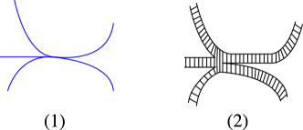
Figure 2. (1) Train track near vertex. (2) Fibered neighborhood.

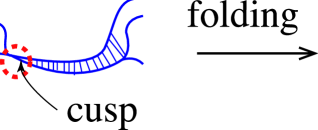
Figure 3. Folding map near a cusp.

Let $\mathcal{F}$ be a measured foliation on $F$. We say that $\mathcal{F}$ is carried by $\tau$ if $\mathcal{F}$ can be represented by a partial measured foliation whose support is $\mathcal{N}(\tau)$ and which is transverse to the ties.

Let $\sigma$ be a train track on $F$. We say that $\sigma$ is carried by $\tau$ if $\sigma$ is isotopic to a train track $\sigma^{\prime}$ which is contained in $\mathcal{N}(\tau)$ and which is transverse to the ties (said differently, every smooth edge path on $\sigma^{\prime}$ is transverse to the ties). Let $f:F\rightarrow F$ be a homeomorphism. A train track $\tau$ is invariant under $[f]$ if $f(\tau)$ is carried by $\tau$, that is, $f(\tau)$ is isotopic to some train track $\sigma^{\prime}$ which satisfies above. In this case, folding edges of $\tau^{\prime}$ near cusps repeatedly (see Figure 3 for a folding map), in other words, collapsing $\tau^{\prime}$ onto $\tau$ smoothly yields a map $\mathfrak{p}:\tau\rightarrow\tau$ such that $\mathfrak{p}$ maps vertices to vertices, and $\mathfrak{p}$ is locally injective at any points which do not map into vertices. Such a $\mathfrak{p}:\tau\rightarrow\tau$ is called a train track representative of $[f]$. An edge $e$ of $\tau$ is said to be infinitesimal (for $\mathfrak{p}$) if $e$ is eventually periodic under $\mathfrak{p}$, that is $\mathfrak{p}^{m+n}(e)=\mathfrak{p}^{n}(e)$ for some positive integers $m$ and $n$. Other edges of $\tau$ is said to be real. Let $k$ be the number of the real edges of $\tau$. Then we have a $k\times k$ non-negative integer matrix $M_{\mathfrak{p}}=(m_{ij})$, called the incidence matrix for $\mathfrak{p}:\tau\rightarrow\tau$ (with respect to real edges), where $m_{ij}$ is the number of times so that the image $\mathfrak{p}(e_{j})$ of the $j$th real edge passes through the $i$th real edge $e_{i}$ in either direction. Also, $\mathfrak{p}:\tau\rightarrow\tau$ determines a finite, directed graph $\Gamma_{\mathfrak{p}}$ by taking a vertex for each real edge of $\tau$, and then adding $m_{ij}$ directed edges from the $j$th real edge $e_{j}$ to the $i$th real edge $e_{i}$. In other words, we have $m_{ij}$ directed edges from $e_{j}$ to $e_{i}$ if $\mathfrak{p}(e_{j})$ passes through $e_{i}$ in either direction $m_{ij}$ times . We say that $\Gamma_{\mathfrak{p}}$ is the induced directed graph of $\mathfrak{p}:\tau\rightarrow\tau$.

A non-negative integer matrix $M$ is said to be Perron-Frobenius if there exists an integer $\ell\geq 1$ such $M^{\ell}$ is positive, that is each entry of $M^{\ell}$ is positive. In this case, the spectral radius of $M$ is given by the largest eigenvalue of $M$ called the Perron-Frobenius eigenvalue, see [8].

The following theorem is well known.

Theorem 2.1 (See Theorem 4.1 in [33] and its proof.).

If $\Phi:F\rightarrow F$ is a pseudo-Anosov homeomorphism, then there exists a train track $\tau$ on $F$ which carries the unstable foliation $\mathcal{F}^{u}$ of $\Phi$ and a train track representative $\mathfrak{p}:\tau\rightarrow\tau$ of $\phi=[\Phi]$. Such a representative $\mathfrak{p}:\tau\rightarrow\tau$ satisfies that the incidence matrix $M_{\mathfrak{p}}$ is Perron-Frobenius and its Perron-Frobenius eigenvalue is exactly equal to $\lambda(\Phi)$.

Conversely, if $f:F\rightarrow F$ is a homeomorphism and if $\mathfrak{p}:\tau\rightarrow\tau$ is a train track representative of $\phi=[f]$ such that its incidence matrix $M_{\mathfrak{p}}$ is Perron-Frobenius, then $\phi$ is pseudo-Anosov whose dilatation $\lambda(\phi)$ equals the Perron-Frobenius eigenvalue of $M_{\mathfrak{p}}$, see Bestvina-Handel [2, Section 3.4]

2.2. Thurston norm, fibered face, entropy function

We review the basic results on Thurston norm and the relation between Thurston norm and hyperbolic, fibered $3$-manifolds developed by Thurston, Fried, Matsumoto and McMullen. Let $M$ be an oriented hyperbolic $3$-manifold possibly $\partial M\neq\emptyset$. We recall Thurston norm $\|\cdot\|:H_{2}(M,\partial M;{\mathbb{R}})\rightarrow{\mathbb{R}}$. For more detail, see [35]. Let $F=F_{1}\cup F_{2}\cup\cdots\cup F_{k}$ be a finite union of oriented, connected surfaces. We define $\chi_{-}{(F)}$ to be

$$\chi_{-}(F)=\sum_{i=1}^{k}\max\{0,-\chi(F_{i})\}.$$

Thurston norm $\|\cdot\|$ is defined for an integral class $a\in H_{2}(M,\partial M;{\mathbb{Z}})$ by

$$\|a\|=\min_{F}\{\chi_{-}(F)\},$$

where the minimum is taken over all oriented surfaces $F$ embedded in $M$ satisfying $a=[F]$. The surface $F$ which realizes the minimum is called a minimal representative of $a$. Then $\|\cdot\|$ admits a unique continuous extension $\|\cdot\|:H_{2}(M,\partial M;{\mathbb{R}})\rightarrow{\mathbb{R}}$ which is linear on rays through the origin. It is known that the unit ball $U_{M}\subset H_{2}(M,\partial M;{\mathbb{R}})$ with respect to Thurston norm $\|\cdot\|$ is a compact, convex polyhedron [35].

Let $\Omega$ be any top dimensional face on the boundary $\partial U_{M}$ of Thurston norm ball. We denote by $C_{\Omega}$, the cone over $\Omega$ with the origin, and we denote by $int(C_{\Omega})$, the interiors of $C_{\Omega}$. Thurston proved in [35] that if $M$ is a surface bundle over the circle and if $F$ be any fiber of the fibration on $M$, then there exists a top dimensional face $\Omega$ on $\partial U_{M}$ so that $[F]$ is an integral class of $int(C_{\Omega})$. Moreover for any integral class $a\in int(C_{\Omega})$, its minimal representative $F_{a}$ becomes a fiber of a fibration on $M$, and $F_{a}$ is unique up to isotopy along flow lines. Such a face $\Omega$ is called an fibered face and an integral class $a\in int(C_{\Omega})$ is called a fibered class. Thus, if the second Betti number $b_{2}(M)$ is greater than $1$, then the single $3$-manifold $M$ provides infinitely many pseudo-Anosovs on surfaces with different topological types.

Let $\Omega$ be a fibered face of $M$. If $a\in int(C_{\Omega})$ is primitive and integral, then the minimal representative $F_{a}$ is a connected fiber of the fibration associated $a$. The mapping class $\phi_{a}=[\Phi_{a}]$ of the monodromy $\Phi_{a}:F_{a}\rightarrow F_{a}$ of its fibration is pseudo-Anosov (since $M$ is hyperbolic). We define the dilatation $\lambda(a)$ and entropy $\mathrm{ent}(a)$ to be the dilatation and entropy of the pseudo-Anosov $\phi_{a}$. The entropy function defined on primitive fibered classes is naturally extended to rational classes. In fact for a rational number $r$ and a primitive fibered class $a$, the entropy of $\mathrm{ra}$ is defined to be $\mathrm{ent}(ra)=\tfrac{1}{|r|}\mathrm{ent}(a)$.

Theorem 2.2 ([7, 27, 28]).

The function given by $a\mapsto\mathrm{ent}(a)$ for each rational class $a\in int(C_{\Omega})$ extends to a real analytic convex function on $int(C_{\Omega})$. The restriction $\mathrm{ent}|_{int(\Omega)}:int(\Omega)\rightarrow{\mathbb{R}}$ is a strictly convex function which goes to $\infty$ toward the boundary of $\Omega$.

By properties of $\|\cdot\|$ and $\mathrm{ent}$, we see that the normalized entropy function

$$\mathrm{Ent}=\|\cdot\|\mathrm{ent}:int(C_{\Omega})\rightarrow{\mathbb{R}}$$

is constant on each ray in $int(C_{\Omega})$ through the origin.

We choose $\phi=[\Phi]\in\mathrm{Mod}(\varSigma)$, and we consider the mapping torus ${\mathbb{T}}_{\phi}$ with the suspension flow $\Phi^{t}$. Hereafter we fix the orientation of $\varSigma$ so that its normal direction coincides with the flow direction of $\Phi^{t}$. For $S\subset\varSigma$, we define $S^{t}\subset{\mathbb{T}}_{\phi}$ to be the image of $S\times\{t\}\subset\varSigma\times\{t\}$ under the projection $p:\varSigma\times{\mathbb{R}}\rightarrow{\mathbb{T}}_{\phi}$.

Theorem 2.3 (Theorem 7 and Lemma in [6]).

Let $\Phi:F\rightarrow F$ be a pseudo-Anosov homeomorphism with stable and unstable foliations $\mathcal{F}^{s}$ and $\mathcal{F}^{u}$ on an oriented surface $F$, and let $\phi=[\Phi]$. Let $\widehat{\mathcal{F}^{s}}$ and $\widehat{\mathcal{F}^{u}}$ denote the suspension of $\mathcal{F}^{s}$ and $\mathcal{F}^{u}$ by $\Phi$. If $\Omega$ is a fibered face on ${\mathbb{T}}_{\phi}$ with $[F]\in int(C_{\Omega})$, then for any minimal representative $F_{a}$ of any fibered class $a\in int(C_{\Omega})$, we can modify $F_{a}$ by isotopy which satisfies the followings.

1. $F_{a}$ is transverse to the flow $\Phi^{t}$, and the first return map $:F_{a}\rightarrow F_{a}$ is precisely the pseudo-Anosov monodromy $\Phi_{a}:F_{a}\rightarrow F_{a}$ of the fibration on ${\mathbb{T}}_{\phi}$ associated to $a$. Moreover $F_{a}$ is unique up to isotopy along flow lines.

2. The stable and unstable foliations of $\Phi_{a}$ are given by $\widehat{\mathcal{F}^{s}}\cap F_{a}$ and $\widehat{\mathcal{F}^{u}}\cap F_{a}$.

Following [30], we introduce flowbands in ${\mathbb{T}}_{\phi}$.

Definition 2.4.

Let $J_{1}$ and $J_{2}$ be embedded arcs in ${\mathbb{T}}_{\phi}$. Suppose that $J_{1}$ and $J_{2}$ are transverse to $\Phi^{t}$. We say that $J_{1}$ is connected to $J_{2}$ (with respect to $\Phi^{t}$) if there exists a positive continuous function $\mathfrak{t}:J_{1}\rightarrow{\mathbb{R}}$ such that for any $x\in J_{1}$, we have

• $\Phi^{\mathfrak{t}(x)}(x)\in J_{2}$, $\Phi^{t}(x)\not\in J_{2}$ for $0<t<\mathfrak{t}(x)$, and

• the map $J_{1}\to J_{2}$ given by $x\mapsto\Phi^{\mathfrak{t}(x)}(x)$ is a homeomorphism.

The flowband $[J_{1},J_{2}]$ is defined by

$$[J_{1},J_{2}]=\{\Phi^{t}(x)\ |\ x\in J_{1},\ 0\leq t\leq\mathfrak{t}(x)\}.$$

Flowbands are used to build branched surfaces in Section 3.3.

2.3. Clique polynomials

We review some results on clique polynomials, developed by McMullen [29]. As we will see in Section 3.7, clique polynomials are useful to compute the dilatations of pseudo-Anosov monodromies of fibrations on fibered $3$-manifolds.

Let $(\Gamma,m)$ be a finite, directed graph $\Gamma$ with a metric $m:E(\Gamma)\rightarrow{\mathbb{R}}_{+}$ on the set of edges $E(\Gamma)$. The metric $m$ specifies the length of each edge. Parallel edges and loops are allowed. We sometimes denote $(\Gamma,m)$ by $\Gamma$ when $m$ is obvious. The growth rate $\lambda(\Gamma,m)$ is defined by

$$\lambda(\Gamma,m)=\lim_{T\to\infty}N_{0}(T)^{1/T},$$

where $N_{0}(T)$ is the number of the closed, directed paths in $\Gamma$ of length $\leq T$.

When $m(e)$ is an integer for each $e\in E(\Gamma)$, we can add $m(e)-1$ new vertices along each edge $e$ to obtain a new directed graph $\Gamma^{\prime}$ with the metric ${\bf 1}:E(\Gamma^{\prime})\rightarrow{\mathbb{R}}_{+}$ sending each edge to $1$. Then we have

$$\lambda(\Gamma,m)=\lambda(\Gamma^{\prime},{\bf 1}).$$

Suppose that $\phi$ is a pseudo-Anosov mapping class. Let $\mathfrak{p}:\tau\rightarrow\tau$ be a train track representative of $\phi$ given in Theorem 2.1 and let $\Gamma_{\mathfrak{p}}$ be the induced directed graph of $\mathfrak{p}:\tau\rightarrow\tau$. Theorem 2.1 implies that $(\Gamma_{\mathfrak{p}},{\bf 1})$ satisfies

(2.1) $$\lambda(\phi)=\lambda(\Gamma_{\mathfrak{p}},{\bf 1}).$$

Let $G$ be a finite, undirected graph with no loops or parallel edges. Let $w:V(G)\rightarrow{\mathbb{R}}_{+}$ be a weight on the set of vertices $V(G)$. The subset $K\subset V(G)$ forms a clique if they span a complete subgraph. (We allow $K=\emptyset$.) The clique polynomial of $(G,w)$ is defined by

$$Q(t)=\sum_{K}(-1)^{(\sharp K)}t^{w(K)},$$

where $\sharp K$ denotes the cardinality of $K$, the weight of $K$ is given by $w(K)=\sum_{v\in K}w(v)$, and the sum is over all cliques $K$’s of $G$. We sometimes denote the weighted, undirected graph $(G,w)$ by $G$ when $w$ is obvious.

McMullen relates the growth rates $\lambda(\Gamma,m)$’s to the clique polynomials via the curve complexes of $(\Gamma,m)$’s. Let $C\subset E(\Gamma)$ be a collection of edges which form a closed, directed loop. If $C$ never visits the same vertex twice, then $C$ is called a simple curve. A multicurve is a finite union of simple curves such that no two simple curves share a vertex. The curve complex of $(\Gamma,m)$ is the undirected graph $G$ together with the weight $w:V(G)\rightarrow{\mathbb{R}}_{+}$, which is obtained by taking a vertex for each simple curve $C$ of $\Gamma$, and then joining the two vertices $C_{1}$ and $C_{2}$ by an edge when $(C_{1},C_{2})$ is a multicurve of $\Gamma$. Then the metric $m$ on $E(\Gamma)$ induces the weight $w$ on $V(G)$ as follows.

$$w(C)=\sum_{e\in C}m(e).$$

Theorem 2.5 ([29]).

Let $(G,w)$ be the curve complex of $(\Gamma,m)$. Then $\tfrac{1}{\lambda(\Gamma,m)}$ is equal to the the smallest positive root of the clique polynomial $Q(t)$ of $(G,w)$.

By (2.1) and Theorem 2.5, we can compute the dilatations of pseudo-Anosovs by using the clique polynomials of curve complexes associated to the pseudo-Anosovs. We do not need to compute the characteristic polynomials of the incidence matrices for the dilatations. This observation is due to Birman [3].

2.4. Fibered classes of the magic manifold $N$

In this section, we review some properties on $N$ which will be used in the paper. We give orientations of components, $K_{1}$, $K_{2}$ and $K_{3}$ of the $3$ chain link $\mathcal{C}_{3}$ as in Figure 1(1). Each component bounds oriented $2$-punctured disks, $F_{\alpha}$, $F_{\beta}$ and $F_{\gamma}$ respectively. We set $\alpha=[F_{\alpha}]$, $\beta=[F_{\beta}]$, $\gamma=[F_{\gamma}]\in H_{2}(N,\partial N;{\mathbb{Z}})$. Then $\{\alpha,\beta,\gamma\}$ becomes a basis of $H_{2}(N,\partial N;{\mathbb{Z}})$. We denote the class $x\alpha+y\beta+z\gamma\in H_{2}(N,\partial N)$ by $(x,y,z)$. Thurston norm ball $U_{N}$ is the parallelepiped with vertices $\pm\alpha=\pm(1,0,0)$, $\pm\beta=\pm(0,1,0)$, $\pm\gamma=\pm(0,0,1)$ and $\pm\alpha+\beta+\gamma=\pm(1,1,1)$ ([35, Example 3]), see Figure 5(1). (Note that the minimal representative of $\kappa$ is taken to be the $3$-punctured sphere, embedded in $S^{3}\setminus\mathcal{C}_{3}$, which contains the point $\infty\in S^{3}\setminus\mathcal{C}_{3}$.)

Let $\mathrm{br}(\sigma_{1}^{2}\sigma_{2}^{-1})$ be the $3$ components link in $S^{3}$ as in Figure 1(2), i.e, it is the link obtained from the closed $3$-braid $\sigma_{1}^{2}\sigma_{2}^{-1}$ together with the braid axis. Then $N=S^{3}\setminus C_{3}$ is homeomorphic to $S^{3}\setminus\mathrm{br}(\sigma_{1}^{2}\sigma_{2}^{-1})$, see Lemma 2.6(1). This implies that $N$ is a surface bundle over the circle with a fiber of the $4$-punctured sphere. Notice that every top dimensional face of $\partial U_{N}$ is a fibered face, because of the symmetries of $\mathcal{C}_{3}$. To study monodromies of fibrations on $N$, we can pick a particular fibered face, for example the fibered face $\Delta$ with vertices $(1,0,0)$, $(1,1,1)$, $(0,1,0)$ and $(0,0,-1)$, see Figure 5(1). The open face $int(\Delta)$ is written by

(2.2) $$int(\Delta)=\{(x,y,z)\ |\ x+y-z=1,\ x>0,\ y>0,\ x>z,\ y>z\}.$$

Thurston norm $\|a\|$ of $a=(x,y,z)\in C_{\Delta}$ is given by $x+y-z$. An integral class $(x,y,z)\in C_{\Delta}$ is fibered (i.e, an integral class $(x,y,z)$ is in $int(C_{\Delta)}$) if and only if $x$, $y$ and $z$ are integers such that $x>0$, $y>0$, $x>z$ and $y>z$, see (2.2).

Any class $a=(x,y,z)\in\Delta$ satisfies $z=x+y-1$. Hence we can write such a class $a=(x,y,z)$ by $[x,y]$. Then we have

$$int(\Delta)=\{[x,y]\ |\ 0<x<1,\ 0<y<1\},$$

see Figure 5(2).

We denote by $T_{\alpha}$ the torus which is the boundary of a regular neighborhood of $K_{1}$. Let $a=(x,y,z)\in int(C_{\Delta})$ be a primitive integral class. We set $\partial_{\alpha}F_{a}=\partial F_{a}\cap T_{\alpha}$ which consists of the parallel simple closed curves on $T_{\alpha}$. We define $T_{\beta}$, $\partial_{\beta}F_{a}$ and $T_{\gamma}$, $\partial_{\gamma}F_{a}$ in a similar way.

Lemma 2.6 ([18] for (1)(3)(5), [19] for (6)(7), [17] for (4)).

Suppose that $a=(x,y,z)\in int(C_{\Delta})$ is a primitive integral class.

• There is an orientation preserving homeomorphism $:S^{3}\setminus\mathcal{C}_{3}\rightarrow S^{3}\setminus\mathrm{br}(\sigma_{1}^{2}\sigma_{2}^{-1})$ which sends the minimal representative $F_{\alpha+\beta}$ associated to $\alpha+\beta$ to the oriented $3$-punctured disk bounded by the braid axis $K_{3}^{\prime}$ as in Figure 4(4). Thus the pseudo-Anosov homeomorphism which represents the mapping class of $\mathrm{Mod}(\varSigma_{0,4})$ corresponding to $\sigma_{1}^{2}\sigma_{2}^{-1}$ becomes the monodromy $\Phi_{\alpha+\beta}:F_{\alpha+\beta}\rightarrow F_{\alpha+\beta}$ of the fibration associated to $\alpha+\beta$.

• The boundary slope of $\partial_{\alpha}F_{a}$ (resp. $\partial_{\beta}F_{a}$, $\partial_{\gamma}F_{a}$) is given by $\tfrac{y+z}{-x}$ (resp. $\tfrac{z+x}{-y}$, $\tfrac{x+y}{-z}$).

• We have $\|a\|=x+y-z$. The number of the boundary components of $F_{a}$ is computed as follows.

  $$\sharp(\partial_{\alpha}F_{a})=\gcd(x,y+z),\ \sharp(\partial_{\beta}F_{a})=\gcd(y,z+x),\ \sharp(\partial_{\gamma}F_{a})=\gcd(z,x+y),$$

  where $\gcd(0,w)$ is defined by $|w|$.

• Let $\Phi_{(x,y,z)}:F_{(x,y,z)}\rightarrow F_{(x,y,z)}$ be the monodromy of the fibration on $N$ associated to $(x,y,z)\in int(C_{\Delta})$. Then $(y,x,z)\in int(C_{\Delta})$, and $(\Phi_{(x,y,z)})^{-1}$ is conjugate to $\Phi_{(y,x,z)}$.

• The dilatation $\lambda(a)=\lambda_{(x,y,z)}$ is the largest root of

  $$f_{(x,y,z)}(t)=t^{x+y-z}-t^{x}-t^{y}-t^{x-z}-t^{y-z}+1.$$

• The (un)stable foliation $\mathcal{F}_{a}$ of $\Phi_{a}$ has a property such that each component of $\partial_{\alpha}F_{a}$, $\partial_{\beta}F_{a}$ and $\partial_{\gamma}F_{a}$ has $\tfrac{x}{\gcd(x,y+z)}$ prongs, $\tfrac{y}{\gcd(y,x+z)}$ prongs and $\tfrac{x+y-2z}{\gcd(z,x+y)}$ prongs respectively. Moreover $\mathcal{F}_{a}$ does not have singularities in the interior of $F_{a}$.

• $\mathcal{F}_{a}$ is an orientable foliation if and only if $x$ and $y$ are even and $z$ is odd.

The proof of (2) is easy. For the convenience of the proof of Lemma 3.4, we prove the claim (1).

Proof of Lemma 2.6(1).

First of all, we observe that the link in Figure 4(2) is isotopic to ${\mathcal{C}}_{3}$ given in Figure 4(1). Observe also that the link in Figure 4(3) is isotopic to the braided link $\mathrm{br}(\sigma_{1}^{2}\sigma_{2}^{-1})$ given in Figure 4(4). We use the link diagrams in (2) and (3). We cut the twice punctured disk ($\simeq F_{\alpha}$) bounded by the component $K_{1}$. Let $F_{\alpha}^{1}$ and $F_{\alpha}^{2}$ be the resulting twice punctured disks obtained from $F_{\alpha}$. We reglue these twice punctured disks twisting either $F_{\alpha}^{1}$ or $F_{\beta}^{2}$ by 360 degrees. Then we obtain the link in (3) which is isotopic to $\mathrm{br}(\sigma_{1}^{2}\sigma_{2}^{-1})$. This implies that there exists an orientation preserving homeomorphism $h:S^{3}\setminus{\mathcal{C}}_{3}\rightarrow S^{3}\setminus\mathrm{br}(\sigma_{1}^{2}\sigma_{2}^{-1})$. Then one can check that $h$ sends the minimal representative of $\alpha+\beta$ to the desired $3$-punctured disk. ∎

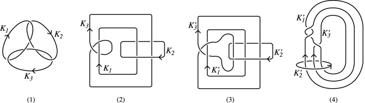
Figure 4. (1)(2) $3$ chain link $\mathcal{C}_{3}$, (3)(4) Braided link $\mathrm{br}(\sigma_{1}^{2}\sigma_{2}^{-1})$.

Lemma 2.6(4) allows us to focus on only fibered classes $(x,y,z)\in int(C_{\Delta})$ such that $y\geq x$ for the proof of Theorem 1.2. We now introduce two bases $\{-\gamma,\beta,\alpha+\beta\}$ and $\{\alpha+\beta+\gamma,\beta,\alpha+\beta\}$ of $H_{2}(N,\partial N,{\mathbb{Z}})$ to describe such fibered classes $(x,y,z)$. If $z\leq 0$ (resp. $z\geq 0$), then we represent $(x,y,z)$ by the base $\{-\gamma,\beta,\alpha+\beta\}$ (resp. $\{\alpha+\beta+\gamma,\beta,\alpha+\beta\}$ ). Let us define

$$\Delta_{+} = \{(x,y,z)\in\Delta\ |\ y\geq x,\ z\geq 0\},$$

$$\Delta_{-} = \{(x,y,z)\in\Delta\ |\ y\geq x,\ z\leq 0\},$$

$$\Delta_{0} = \{(x,y,z)\in\Delta\ |\ y\geq x,\ z=0\},$$

see Figure 5(3)(4), and define $\widehat{\Delta}_{\pm}\subset\Delta_{\pm}$ as follows.

$$\widehat{\Delta}_{+} = \{(x,y,z)\in\Delta\ |\ x=y,\ z\geq 0\},$$

$$\widehat{\Delta}_{-} = \{(x,y,z)\in\Delta\ |\ x=y,\ z\leq 0\},$$

see Figure 5(4). For non-negative integers $i,j$ and $k$, we define integral classes $(i,j,k)_{\pm}$, $(j,k)_{0}\in C_{\Delta}$ to be

$$(i,j,k)_{+} = i(1,1,1)+j(0,1,0)+k(1,1,0)=(i+k,i+j+k,i),$$

$$(i,j,k)_{-} = i(0,0,-1)+j(0,1,0)+k(1,1,0)=(k,j+k,-i),$$

$$(j,k)_{0} = (0,j,k)_{+}=(0,j,k)_{-},$$

where $(1,1,1)=\alpha+\beta+\gamma$, $(0,0,-1)=-\gamma$, $(0,1,0)=\beta$, and $(1,1,0)=\alpha+\beta$. The classes $(i,j,k)_{\pm}$ with $i,j,k>0$ are said to be non-degenerate. Other classes $(i,j,k)_{\pm}$ are said to be degenerate. Note that an integral class $(i,j,k)_{\pm}$ is fibered if and only if $i$, $j$ are non-negative integers and $k$ is a positive integer, see (2.2). If a fibered class $(x,y,z)\in int(C_{\Delta})$ satisfies $y\geq x$ and $z\leq 0$ (resp. $y\geq x$ and $z\geq 0$), then $(x,y,z)$ is written by $(i,j,k)_{+}$ (resp. $(i,j,k)_{-}$) for some $i,j\geq 0$ and $k\geq 1$.

We use the notations $f_{(i,j,k)_{\pm}}$ and $\lambda_{(i,j,k)_{\pm}}$ in the same manner as $f_{(x,y,z)}$ and $\lambda_{(x,y,z)}$ appeared in Lemma 2.6. We denote by $[a]$, the projection of $a$ to the fibered face $\Delta$. For simplicity, we write $[(i,j,k)_{\pm}]=[i,j,k]_{\pm}$ and $[(j,k)_{0}]=[j,k]_{0}$. Clearly $[i,j,k]_{\pm}\in\Delta_{\pm}$ and $[j,k]_{0}\in\Delta_{0}$. By claims (2)(3) in the following lemma, we find that coordinates $(i,j,k)_{\pm}$ are useful to study symmetries of the entropy function on $N$.

Lemma 2.7.

Let $a=(i,j,k)_{\pm}\in int(C_{\Delta})$ be a primitive integral class.

• The dilatation $\lambda_{(i,j,k)_{\pm}}$ is the largest root of

  $$f_{(i,j,k)_{\pm}}(t)=t^{i+j+2k}-t^{k}-t^{i+k}-t^{j+k}-t^{i+j+k}+1.$$

  In particular $\lambda_{(i,j,k)_{+}}=\lambda_{(i,j,k)_{-}}$.

• The integral class $(j,i,k)_{\pm}$ is a fibered class in $int(C_{\Delta})$, and the equality $f_{(i,j,k)_{\pm}}=f_{(j,i,k)_{\pm}}$ holds. In particular, $\lambda_{(i,j,k)_{\pm}}=\lambda_{(j,i,k)_{\pm}}$.

• Two classes $[i,j,k]_{+}$ and $[j,i,k]_{+}$ have a line symmetry about $x=\frac{1}{2}$, and $[i,j,k]_{+}$ and $[i,j,k]_{-}$ have a line symmetry about $y=-x+1$, see Figure 5(5)(6).

Proof.

The claim (1) holds by Lemma 2.6(5). The first part of (2) follows from (2.2). The second part of (2) is obvious from the claim (1). The proof of (3) is easy to check. (cf. Corollary 2.7 and Remark 2.8 in [17].) ∎

Although all fibered classes $(i,j,k)_{\pm}$ and $(j,i,k)_{\pm}$ have the same Thurston norm $i+j+2k$ and same dilatation, the topological types of their fibers could be different in general. To see what the pseudo-Anosovs $\Phi_{(i,j,k)_{\pm}}$ and $\Phi_{(j,i,k)_{\pm}}$ look like, we will see the curve complexes associated to $(i,j,k)_{\pm}$ and $(j,i,k)_{\pm}$ in Section 3.7.

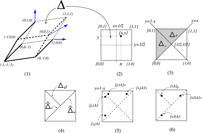
Figure 5. (1) Thurston norm ball $U_{N}$ and the fibered face $\Delta$. (2) $[x,y]\in\Delta$. (3) $\Delta_{\pm}$. (4) $\Delta_{0}$, $\widehat{\Delta}_{\pm}$. (5) Projective classes of non-degenerate $[i,j,k]_{\pm}$ and $[j,i,k]_{\pm}$. (6) Projective classes of degenerate $[i,0,k]_{\pm}$ and $[i,k]_{0}=[0,i,k]_{\pm}$.

3. Construction

In Section 3.1, we construct the pseudo-Anosov homeomorphism on $\varSigma_{0,4}$ which represents the mapping class corresponding to the $3$-braid $\sigma_{1}^{2}\sigma_{2}^{-1}$. It serves the monodromy $\Phi_{\alpha+\beta}:F_{\alpha+\beta}\rightarrow F_{\alpha+\beta}$ of the fibration on $N$ associated to $\alpha+\beta$, and plays a rule as a pseudo-Anosov homeomorphism $\Phi$ in Theorem 2.3. We also construct a train track representative $\mathfrak{p}_{\alpha+\beta}:\tau_{\alpha+\beta}\rightarrow\tau_{\alpha+\beta}$ of $\phi_{\alpha+\beta}=[\Phi_{\alpha+\beta}]$.

Oertel used branched surfaces to describe Thurston norm and to study fibers of fibrations on hyperbolic, fibered $3$-manifolds. For basic definitions and results on branched surfaces, see [24, 31, 32]. In Section 3.2, we find minimal representatives of non-fibered classes $\alpha$, $\beta$, $\kappa_{\pm}$, where $\kappa_{+}=\alpha+\beta+\gamma$ and $\kappa_{-}=-\gamma$. In Section 3.3, by using minimal representatives found in Section 3.2, we build two branched surfaces $\mathcal{B}_{\pm}$ which carry fibers $F_{(i,j,k)_{\pm}}$ of fibrations associated to any fibered class $(i,j,k)_{\pm}$. Then in Section 3.4, we construct the train track $\tau_{(i,j,k)_{\pm}}$ which carries the unstable foliation $\mathcal{F}_{(i,j,k)_{\pm}}$ of the pseudo-Anosov monodromy $\Phi_{(i,j,k)_{\pm}}:F_{(i,j,k)_{\pm}}\rightarrow F_{(i,j,k)_{\pm}}$ of the fibration associated to $(i,j,k)_{\pm}$. In Section 3.5, we construct the the pseudo-Anosov $\Phi_{(i,j,k)_{\pm}}:F_{(i,j,k)_{\pm}}\rightarrow F_{(i,j,k)_{\pm}}$ explicitly. In Section 3.6, we give an explicit construction of the train track representative $\mathfrak{p}_{(i,j,k)_{\pm}}:\tau_{(i,j,k)_{\pm}}\rightarrow\tau_{(i,j,k)_{\pm}}$ for $\phi_{(i,j,k)_{\pm}}=[\Phi_{(i,j,i)_{\pm}}]$. We also construct the directed graph $\Gamma_{(i,j,k)_{\pm}}$ induced by $\mathfrak{p}_{(i,j,k)_{\pm}}:\tau_{(i,j,k)_{\pm}}\rightarrow\tau_{(i,j,k)_{\pm}}$ to indicate where each real edge of $\tau_{(i,j,k)_{\pm}}$ maps to under $\mathfrak{p}_{(i,j,k)_{\pm}}$. In Section 3.7, we give the curve complex $G_{(i,j,k)_{\pm}}$ of $\Gamma_{(i,j,k)_{\pm}}$ and compute its clique polynomial $Q_{(i,j,k)_{\pm}}(t)$ whose largest root equals the dilatation $\lambda_{(i,j,k)_{\pm}}$.

3.1. Fibered class $\alpha+\beta$

Let $L=L_{\mathcal{M}}:{\mathbb{R}}^{2}\rightarrow{\mathbb{R}}^{2}$ be the linear map induced by $\mathcal{M}=\left(\begin{smallmatrix}3&2\\ 1&1\end{smallmatrix}\right)\in SL(2,{\mathbb{Z}})$. Since $\mathcal{M}$ has eigenvalues $\lambda^{\pm 1}(=2\pm\sqrt{3})$ with $\lambda^{+}>1$ and $0<\lambda^{-1}<1$, the linear map $L$ descends to the Anosov diffeomorphism $f=f_{\mathcal{M}}:{\mathbb{R}}^{2}/{\mathbb{Z}}^{2}\rightarrow{\mathbb{R}}^{2}/{\mathbb{Z}}^{2}$ on the torus. Figure 6 is an illustration of the image of the unit square with the origin (on the left bottom corner) under $L$.

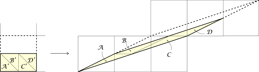
Figure 6. Rectangle $\mathcal{R}$ (left) and its image $L(\mathcal{R})$ (right). (The images of the isosceles right-angled triangles $\mathcal{A}^{\prime}$, $\mathcal{B}^{\prime}$, $\mathcal{C}^{\prime}$ and $\mathcal{D}^{\prime}$ under $L$ are the acute-angled triangles $\mathcal{A}$, $\mathcal{B}$, $\mathcal{C}$ and $\mathcal{D}$.)

The linear map induced by $\left(\begin{smallmatrix}-1&0\\ 0&-1\end{smallmatrix}\right)\in SL(2,{\mathbb{Z}})$ defines a reflection $\mathfrak{r}:{\mathbb{R}}^{2}/{\mathbb{Z}}^{2}\rightarrow{\mathbb{R}}^{2}/{\mathbb{Z}}^{2}$. The quotient of ${\mathbb{R}}^{2}/{\mathbb{Z}}^{2}$ by $\mathfrak{r}$, denoted by ${\mathbb{S}}$, is homeomorphic to a sphere. (${\mathbb{S}}$ is called a pillowcase because of its shape.) We set the points $a_{i}=(\frac{i}{2},0)$, $b_{i}=(\frac{i}{2},\frac{1}{2})\in{\mathbb{R}}^{2}$. Let $\mathcal{R}$ be the rectangle $a_{0}a_{2}b_{2}b_{0}$ on ${\mathbb{R}}^{2}$, see Figure 7(1). Then ${\mathbb{S}}$ is obtained from $\mathcal{R}$ by identifying the three pairs of the oriented closed segments $\mathcal{K}=b_{0}b_{1}$ with $\mathcal{K}^{\prime}=b_{2}b_{1}$, $\mathcal{I}^{\prime}=a_{0}b_{0}$ with $\mathcal{I}=a_{2}b_{2}$, and $\mathcal{J}^{\prime}=a_{1}a_{0}$ with $\mathcal{J}=a_{1}a_{2}$, see Figure 7. If we let $\pi:{\mathbb{R}}^{2}\rightarrow{\mathbb{S}}$ be the composition of the projections ${\mathbb{R}}^{2}\rightarrow{\mathbb{R}}^{2}/{\mathbb{Z}}^{2}$ and ${\mathbb{R}}^{2}/{\mathbb{Z}}^{2}\rightarrow{\mathbb{S}}$, then the differentiable structure of ${\mathbb{S}}$ has the four singularities $\mathfrak{b}_{1}=\pi(b_{0})$, $\mathfrak{b}_{2}=\pi(b_{1})$, $\mathfrak{b}_{3}=\pi(a_{1})$ and $\mathfrak{b}_{4}=\pi(a_{0})$ which lie on the corners of ${\mathbb{S}}$. We set ${\mathbb{B}}=\{\mathfrak{b}_{1},\mathfrak{b}_{2},\mathfrak{b}_{3},\mathfrak{b}_{4}\}$.

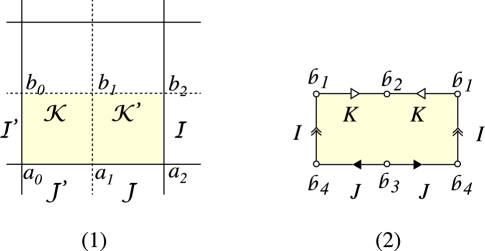
Figure 7. (1) $\mathcal{R}=a_{0}a_{2}b_{2}b_{0}$. (2) $4$-punctured sphere ${\mathbb{S}}\setminus{\mathbb{B}}$.

We have the identity $f\circ\mathfrak{r}=\mathfrak{r}\circ f$, and this implies that $f:{\mathbb{R}}^{2}/{\mathbb{Z}}^{2}\rightarrow{\mathbb{R}}^{2}/{\mathbb{Z}}^{2}$ induces a homeomorphism $\tilde{f}:{\mathbb{S}}\rightarrow{\mathbb{S}}$. Clearly ${\mathbb{B}}$ is invariant under $\tilde{f}$. (More concretely, $\tilde{f}(\mathfrak{b}_{i})=\mathfrak{b}_{i}$ for $i=1,4$, $\tilde{f}(\mathfrak{b}_{2})=\mathfrak{b}_{3}$ and $\tilde{f}(\mathfrak{b}_{3})=\mathfrak{b}_{2}$.) We see that the homeomorphism $\tilde{f}$ on ${\mathbb{S}}$ away from ${\mathbb{B}}$ inherits the (un)stable foliation of the Anosov $f$. Therefore, $f:{\mathbb{R}}^{2}/{\mathbb{Z}}^{2}\rightarrow{\mathbb{R}}^{2}/{\mathbb{Z}}^{2}$ induces a pseudo-Anosov homeomorphism on ${\mathbb{S}}\setminus{\mathbb{B}}\simeq\varSigma_{0,4}$, see Figure 7(2). Abusing the notation, we denote the pseudo-Anosov on ${\mathbb{S}}\setminus{\mathbb{B}}$ by the same notation $\tilde{f}$. Figure 8 is an illustration of $\tilde{f}:\varSigma_{0,4}\rightarrow\varSigma_{0,4}$. (cf. Figure 6.) Let $A^{\prime}$, $B^{\prime}$, $C^{\prime}$ and $D^{\prime}$ be isosceles right-angled triangles whose vertices are punctures of $\varSigma_{0,4}$, see Figure 8(left). Their images under $\tilde{f}$, denoted by $A$, $B$, $C$ and $D$, look as in Figure 8(right).

Observe that the (un)stable foliation of $\tilde{f}$ has a $1$-pronged singularity at each puncture. If we regard the puncture $\mathfrak{b}_{4}$ as the boundary of the $3$-punctured disk, then the mapping class $[\tilde{f}]$ is written by a $3$-braid on the disk. Since $\mathcal{M}$ is of the form $\left(\begin{smallmatrix}1&1\\ 0&1\end{smallmatrix}\right)^{2}\left(\begin{smallmatrix}1&0\\ 1&1\end{smallmatrix}\right),$ we see that $[\tilde{f}]$ is represented by the $3$-braid $\sigma_{1}^{2}\sigma_{2}^{-1}$ (reading the word from the right to the left). Equivalently $[\tilde{f}]$ is written by $(h_{1})^{2}\circ h_{2}^{-1}$, where $h_{i}$ denotes the mapping class which represents the positive half-twist about the segment $\mathfrak{b}_{i}\mathfrak{b}_{i+1}$, see Figure 7(2).

Remark 3.1.

We have a natural homeomorphism $\tilde{h}:\mathrm{br}(\sigma_{1}^{2}\sigma_{2}^{-1})\rightarrow{\mathbb{T}}_{[\tilde{f}]}$. The cusp of the component $K_{2}^{\prime}$ (resp. $K_{1}^{\prime}$) of the link $\mathrm{br}(\sigma_{1}^{2}\sigma_{2}^{-1})$ maps to (under $\tilde{h}$) the cusp corresponding to the orbit of $\mathfrak{b}_{4}$ (resp. $\mathfrak{b}_{1}$) of the suspension flow (see Figure 1(2)). The cusp of the component $K_{3}^{\prime}$ maps to (under $\tilde{h}$) the cusp corresponding to the orbit $\mathfrak{b}_{2}$ (or $\mathfrak{b}_{3}$).

By Lemma 2.6(1) together with Remark 3.1, we can regard $\tilde{f}:\varSigma_{0,4}\rightarrow\varSigma_{0,4}$ as the monodromy $\Phi_{\alpha+\beta}:F_{\alpha+\beta}\rightarrow F_{\alpha+\beta}$ of the fibration on $N$ associated to $\alpha+\beta$. We denote $\tilde{f}$ by $\Phi_{\alpha+\beta}$.

Next we turn to a train track representative of $\phi_{\alpha+\beta}=[\Phi_{\alpha+\beta}]$. Let $\tau_{\alpha+\beta}$ be a train track on $\varSigma_{0,4}$ as in Figure 9(1). Figures 9(1)(5) show that $\tau_{\alpha+\beta}$ is invariant under $\phi_{\alpha+\beta}$. In fact, we have the image $\Phi_{\alpha+\beta}(\tau_{\alpha+\beta})$ in Figure 9(2). (For the illustration of $\Phi_{\alpha+\beta}(\tau_{\alpha+\beta})$, consider the image of the acute-angled triangle $B$, see Figure 8(right).) The train track $\Phi_{\alpha+\beta}(\tau_{\alpha+\beta})$ is isotopic to the one as in Figure 9(5) which is carried by $\tau_{\alpha+\beta}$. As a result, we get the desired train track representative $\mathfrak{p}_{\alpha+\beta}:\tau_{\alpha+\beta}\rightarrow\tau_{\alpha+\beta}$ of $\phi_{\alpha+\beta}$ whose incidence matrix of $\mathfrak{p}_{\alpha+\beta}$ (with respect to the real edges $p$ and $q$) is equal to $\mathcal{M}=\left(\begin{smallmatrix}3&2\\ 1&1\end{smallmatrix}\right)$.

In the rest of the paper, we consider the magic manifold $N$ of the form ${\mathbb{T}}_{\phi_{\alpha+\beta}}=\varSigma_{0,4}\times[0,1]/\sim$, where $\sim$ identifies $x\times\{1\}$ with $\Phi_{\alpha+\beta}(x)\times\{1\}$ for each $x\in\varSigma_{0,4}$. We investigate the suspension flow $\Phi_{\alpha+\beta}^{t}$ on ${\mathbb{T}}_{\phi_{\alpha+\beta}}$. We choose the orientation of ${\mathbb{S}}\setminus{\mathbb{B}}$ so that its normal direction coincides with the flow direction of $\Phi_{\alpha+\beta}^{t}$. We fix the illustration of the $4$-punctured sphere ${\mathbb{S}}\setminus{\mathbb{B}}$ as in Figure 7(2), but we often omit the names of the punctures $\mathfrak{b}_{i}$’s.

Remark 3.2.

Loop edges of $\tau_{\alpha+\beta}$ surrounding punctures $\mathfrak{b}_{1}$, $\mathfrak{b}_{2}$ are $\mathfrak{b}_{3}$ are infinitesimal edges for $\mathfrak{p}_{\alpha+\beta}:\tau_{\alpha+\beta}\rightarrow\tau_{\alpha+\beta}$. Other edges $p$ and $q$ are real edges. Each component of $\varSigma_{0,4}\setminus\tau_{\alpha+\beta}$ is a once punctured monogon. (This comes from the fact that the (un)stable foliation of $\tilde{f}$ has a $1$-pronged singularity at each puncture.) In particular the component of $\varSigma_{0,4}\setminus\tau_{\alpha+\beta}$ containing the puncture $\mathfrak{b}_{4}$ has exactly one cusp.

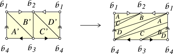
Figure 8. $\tilde{f}(=\Phi_{\alpha+\beta}):\varSigma_{0,4}\rightarrow\varSigma_{0,4}$.

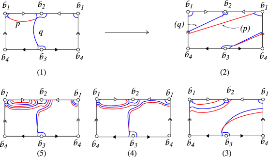
Figure 9. (1) Train track $\tau_{\alpha+\beta}$. (2) The image of $\tau_{\alpha+\beta}$ under $\tilde{f}$, where the image of the edge $p$ etc. is denote by $(p)$ etc. The image $\tilde{f}(\tau_{\alpha+\beta})$ can be put in the tie neighborhood of $\tau_{\alpha+\beta}$ under the isotopy, see (2)$\rightarrow$(3)$\rightarrow$(4)$\rightarrow$(5). (From (4) $\rightarrow$ (5), the edges in (4) that are isotopic to the edges $(p)=\tilde{f}(p)$ and $(q)=\tilde{f}(q)$ in (2) cross over the segment $K$ (see Figure 7(2) for $K$).

3.2. Minimal representatives of $\alpha$, $\beta$, $-\gamma$ and $\alpha+\beta+\gamma$

First we define several sets on ${\mathbb{R}}^{2}$ (see Figure 10(1)). Let $\mathcal{T}_{A}$ and $\mathcal{T}_{B}$ be the triangles $a_{0}b_{2}b_{0}$ and $a_{0}a_{2}b_{2}$ respectively. Let $\mathcal{P}_{K_{-}}$ and $\mathcal{P}_{K_{+}}$ be the parallelograms $a_{0}a_{1}b_{4}b_{3}$ and $a_{1}a_{2}b_{5}b_{4}$ respectively. See Figure 10(1). Note that

$${\mathbb{S}}=\pi(\mathcal{R})=\pi(\mathcal{T}_{A}\cup\mathcal{T}_{B})=\pi(\mathcal{P}_{K_{-}}\cup\mathcal{P}_{K_{+}}),$$

where $\pi:{\mathbb{R}}^{2}\rightarrow{\mathbb{S}}$ is the projection in Section 3.1. Let $\mathcal{U}$ be the oriented closed segment $a_{0}b_{2}$. Let $\mathcal{V}$ and $\mathcal{W}$ be the oriented closed segments $b_{3}a_{0}$ and $b_{4}a_{1}$.

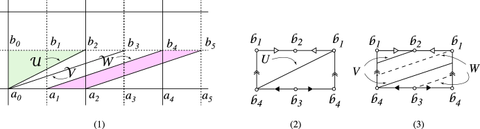
Figure 10. (1) $\mathcal{T}_{A}=a_{0}b_{2}b_{0}$, $\mathcal{T}_{B}=a_{0}a_{2}b_{2}$, $\mathcal{P}_{K_{+}}=a_{1}a_{2}b_{5}b_{4}$, $\mathcal{P}_{K_{-}}=a_{0}a_{1}b_{4}b_{3}$, $\mathcal{U}=a_{0}b_{2}$, $\mathcal{V}=b_{3}a_{0}$, $\mathcal{W}=b_{4}a_{1}$. (2) $U$. (3) $V$, $W$.

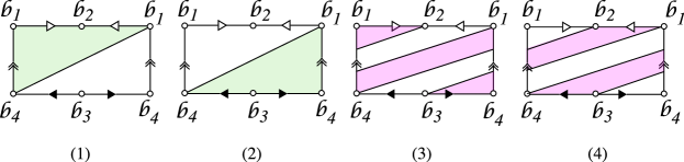
Figure 11. (1) $T_{A}$. (2) $T_{B}$. (3) $P_{K_{+}}$. (4) $P_{K_{-}}$.

Let $T_{A}$ be the image $\pi(\mathcal{T}_{A})\subset{\mathbb{S}}$ removing all points in ${\mathbb{B}}$, i.e, $T_{A}=\pi(\mathcal{T}_{A})\setminus{\mathbb{B}}$. We define $T_{B}$, $P_{K_{+}}$, $P_{K_{-}}\subset{\mathbb{S}}\setminus{\mathbb{B}}$ in the same manner. See Figure 11. Similarly, we let

$$I=\pi(\mathcal{I})\setminus{\mathbb{B}}=\pi(\mathcal{I}^{\prime})\setminus{\mathbb{B}}.$$

Said differently, $I$ is obtained from $\pi(\mathcal{I})=\pi(\mathcal{I}^{\prime})$ by removing the end points. We define $J,K,U,V,W\subset{\mathbb{S}}\setminus{\mathbb{B}}$ in the same manner. See Figures 7(2) and 10(2)(3). We choose the orientations of $T_{A}$, $T_{B}$, $P_{K_{\pm}}$ which coincide with the ones induced by the fiber $F_{\alpha+\beta}={\mathbb{S}}\setminus{\mathbb{B}}$ of the fibration associated to $\alpha+\beta$.

Remark 3.3.

We have $U\cap P_{K_{+}}=U$ and $U\cap P_{K_{+}}=\emptyset$, see Figures 10(2) and 11(3)(4)).

We have $\Phi_{\alpha+\beta}(I)=U$. (We can check the equality by using Figure 6.) This implies that $I^{1}=U^{0}$ in ${\mathbb{T}}_{\phi_{\alpha+\beta}}$, and hence the flowband $[I^{0},U^{0}]$ with respect to $\Phi_{\alpha+\beta}^{t}$ is defined. Let

$$F_{A} = T_{A}^{0}\cup[I^{0},U^{0}],\ \mbox{and}\$$

$$F_{B} = T_{B}^{0}\cup[I^{0},U^{0}],$$

see Figure 12(1)(2). Observe that the both $F_{A}$ and $F_{B}$ are $3$-punctured spheres in ${\mathbb{T}}_{\phi_{\alpha+\beta}}$.

We find two more $3$-punctures spheres $F_{K_{\pm}}$ in ${\mathbb{T}}_{\phi_{\alpha+\beta}}$. Note that $\pi(\mathcal{J})=\pi(\mathcal{J}^{\prime})$ and $\pi(\mathcal{K})=\pi(\mathcal{K}^{\prime})$. We have that $\Phi_{\alpha+\beta}(J)=V$ and $\Phi_{\alpha+\beta}(K)=W$, because $\pi(L(\mathcal{J}))=\pi(\mathcal{V})$ and $\pi(L(\mathcal{K}))=\pi(\mathcal{W})$. Hence $J^{1}=V^{0}$ and $K^{1}=W^{0}$ in ${\mathbb{T}}_{\phi_{\alpha+\beta}}$, and the flowbands $[J^{0},V^{0}]$ and $[K^{0},W^{0}]$ are defined. Let

$$F_{K_{+}} = P_{K_{+}}\cup[J^{0},V^{0}]\cup[K^{0},W^{0}],\ \mbox{and}\$$

$$F_{K_{-}} = P_{K_{-}}\cup[J^{0},V^{0}]\cup[K^{0},W^{0}],$$

see Figure 12(3)(4). We choose the orientations of $F_{A}$, $F_{B}$ and $F_{K_{\pm}}$ so that they are extended by the orientations of $T_{A}^{0}$, $T_{B}^{0}$ and $P_{K_{\pm}}^{0}$. (Here we identify $T_{A}^{0}$ etc. with $T_{A}$ etc.)

Lemma 3.4.

The $3$-punctures spheres $F_{A}$, $F_{B}$, $F_{K_{+}}$ and $F_{K_{-}}$ are minimal representatives of $\alpha$, $\beta$, $\kappa_{+}(=\alpha+\beta+\gamma)$ and $\kappa_{-}(=-\gamma)$ respectively.

Proof of Lemma 3.4.

Let $m_{1}$, $m_{2}$ and $m_{3}$ be the meridians of the components $K_{1}$, $K_{2}$ and $K_{3}$ of the $3$ chain link $\mathcal{C}_{3}$. We take oriented simple closed curves $S_{1}$, $S_{2}$ and $S_{3}$ in ${\mathbb{T}}_{\phi_{\alpha+\beta}}\simeq N$ as in Figure 13. We observe that the images of $m_{1}$, $m_{2}$ and $m_{3}$ under the homeomorphism $H=\tilde{h}\circ h:S^{3}\setminus\mathcal{C}_{3}\rightarrow{\mathbb{T}}_{\alpha+\beta}$ are $S_{1}$, $S_{2}$ and $S_{3}$ respectively (up to isotopy).

Now, we consider the intersections $i(\cdot,\cdot)$ between the surface $F_{B}$ and either $S_{1}$, $S_{2}$ or $S_{3}$. We have $i(F_{B},S_{1})=0$, $i(F_{B},S_{2})=1$, and $i(F_{B},S_{3})=0$. These imply that $F_{B}$ is a minimal representative of $\beta$. By cut and past construction of the union of surfaces $F_{A}\cup F_{B}$, we obtain a surface which is homeomorphic to $F_{\alpha+\beta}={\mathbb{S}}\setminus{\mathbb{B}}$. Since $\beta=[F_{B}]$ and $\alpha+\beta=[F_{\alpha+\beta}]$, we conclude that $F_{A}$ is a minimal representative of $\alpha$.

Let us consider the intersections between $F_{K_{-}}$ and either $S_{1}$, $S_{2}$, or $S_{3}$. We have $i(F_{K_{-}},S_{1})=0$, $i(F_{K_{-}},S_{2})=0$, and $i(F_{K_{-}},S_{3})=-1$. Thus we conclude that $F_{K_{-}}$ is a minimal representative of $-\gamma$. Then we see that $F_{K_{+}}$ is a minimal representative of $\alpha+\beta+\gamma$, because $\alpha+\beta=[F_{\alpha+\beta}]$ and $F_{\alpha+\beta}={\mathbb{S}}\setminus{\mathbb{B}}$ can be obtained from $F_{K_{+}}\cup F_{K-}$ by cut and past construction. ∎

By Lemma 3.4, it makes sense to denote $F_{A}$, $F_{B}$, $F_{K_{+}}$ and $F_{K_{-}}$ by $F_{\alpha}$, $F_{\beta}$, $F_{\kappa_{+}}$ and $F_{\kappa_{-}}$ respectively.

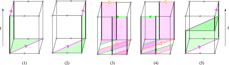
Figure 12. (1)–(5) $3$-punctured spheres embedded in ${\mathbb{T}}_{\phi_{\alpha+\beta}}$ with the suspension flow $\Phi_{\alpha+\beta}^{t}$. The top and bottom surfaces are $\varSigma_{0,4}\times\{1\}$ and $\varSigma_{0,4}\times\{0\}$ respectively. They are identified by $\Phi_{\alpha+\beta}$. Two edges with the same kind (red, green, yellow) are identified in ${\mathbb{T}}_{\phi_{\alpha+\beta}}$. The vertical arrows with the labeling $t$ indicate the flow directions. (1) $F_{\alpha}=F_{A}$. (2) $F_{\beta}=F_{B}$. (3) $F_{\kappa_{+}}=F_{K_{+}}$. (4) $F_{\kappa_{-}}=F_{K_{-}}$. (5) $F_{\beta}^{t}$ for some $0<t<1$.

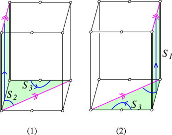
Figure 13. (1) $S_{2}$, $S_{3}$ and $F_{\alpha}$ in ${\mathbb{T}}_{\phi_{\alpha+\beta}}$. (2) $S_{1}$, $S_{3}$ and $F_{\beta}$ in ${\mathbb{T}}_{\phi_{\alpha+\beta}}$.

In the end of this subsection, we introduce surfaces $F_{\beta}^{t}$. We denote by $F_{\beta}^{t}$, the oriented surface in ${\mathbb{T}}_{\phi_{\alpha+\beta}}$ which is obtained from $F_{\beta}$ by pushing $F_{\beta}^{0}$ along the flow direction for $t\geq 0$ times, see Figure 12(5). Clearly $\beta=[F_{\beta}^{t}]$. In the same manner we can define other surfaces $F_{\kappa_{\pm}}^{t}$ and $F_{\alpha+\beta}^{t}$.

3.3. Branched surfaces which carry fibers $F_{(i,j,k)_{\pm}}$

We first construct the branched surface $\mathcal{B}_{+}$. We choose $\delta,\epsilon>0$ so that $0<\delta<2\delta<1-\epsilon$. We consider surfaces $F_{\kappa_{+}}^{\delta}$, $F_{\beta}^{2\delta}$, $F_{\alpha+\beta}^{1-\epsilon}\subset{\mathbb{T}}_{\phi_{\alpha+\beta}}$. We have $\kappa_{+}=[F_{\kappa_{+}}^{\delta}]$, $\beta=[F_{\beta}^{2\delta}]$ and $\alpha+\beta=[F_{\alpha+\beta}^{1-\epsilon}]$. Let

(3.1) $$\widehat{\mathcal{B}}_{+}=F_{\kappa_{+}}^{\delta}\cup F_{\beta}^{2\delta}\cup F_{\alpha+\beta}^{1-\epsilon}\subset{\mathbb{T}}_{\phi_{\alpha+\beta}}.$$

The intersection of each pair of the three surfaces is as follows.

1. $F_{\alpha+\beta}^{1-\epsilon}\cap F_{\beta}^{2\delta}=I^{1-\epsilon}$,

2. $F_{\alpha+\beta}^{1-\epsilon}\cap F_{\kappa_{+}}^{\delta}=J^{1-\epsilon}\cup K^{1-\epsilon}$,

3. $F_{\beta}^{2\delta}\cap F_{\kappa_{+}}^{\delta}=J^{2\delta}\cup U^{\delta}$. (See Remark 3.3 and Figure 12(3)(5).)

The local picture near each intersection looks as in Figure 14(1). A common property of the pairs is that locally, a surface near the intersection is parallel to $F_{\alpha+\beta}$, and it intersects with the flowband which is the subset of the other surface (in fact $F_{\kappa_{+}}^{\delta}$ or $F_{\beta}^{2\delta}$). The branched surface $\mathcal{B}_{+}$ can be obtained from $\widehat{\mathcal{B}}_{+}$ by modifying each flowband of $F_{\kappa_{+}}^{\epsilon}$ and $F_{\beta}^{2\epsilon}$ as in Figure 14(2) so that the modifications agree with the orientations of the two surfaces. Each point in the intersection of surfaces belongs to the branched locus of $\mathcal{B}_{+}$ (that is, the union of points of the branched surface none of whose neighborhood are manifolds).

We build the branched surface $\mathcal{B}_{-}$ in the same manner: Take $F_{\kappa_{-}}^{\delta}$ which represents $\kappa_{-}$ instead of $F_{\kappa_{+}}^{\delta}$. Let

(3.2) $$\widehat{\mathcal{B}}_{-}=F_{\kappa_{-}}^{\delta}\cup F_{\beta}^{2\delta}\cup F_{\alpha+\beta}^{1-\epsilon}\subset{\mathbb{T}}_{\phi_{\alpha+\beta}}.$$

We have

1. $F_{\alpha+\beta}^{1-\epsilon}\cap F_{\beta}^{2\delta}=I^{1-\epsilon}$,

2. $F_{\alpha+\beta}^{1-\epsilon}\cap F_{\kappa_{-}}^{\delta}=J^{1-\epsilon}\cup K^{1-\epsilon}$,

3. $F_{\beta}^{2\delta}\cap F_{\kappa_{-}}^{\delta}=J^{2\delta}$. (See Remark 3.3 and Figure 12(4)(5).)

The branched surface $\mathcal{B}_{-}$ is obtained from $\widehat{\mathcal{B}}_{-}$ by modifying each flowband of $F_{\kappa_{-}}^{\epsilon}$ and $F_{\beta}^{2\epsilon}$ in the similar manner as in the construction of $\mathcal{B}_{+}$.

Figure 16(1) (resp. Figure 16(3)) illustrates three pieces (bottom, middle, top) for building $\mathcal{B}_{+}$ (resp. $\mathcal{B}_{-}$). In this figure, we have two kinds (solid/broken) of segments without arrows and two kinds (solid/broken) of segments with arrows. The broken segments without arrows are parts of the orbits of punctures $\mathfrak{b}_{1}$, $\mathfrak{b}_{2}$, $\mathfrak{b}_{3}$ and $\mathfrak{b}_{4}$ (which are circles in the figure) under the flow. In other words, they lie on the cusps of ${\mathbb{T}}_{\phi_{\alpha+\beta}}\simeq N$. We now explain our convention of Figure 16(1)(3). Firstly, there are some pairs of segments with the same labeling. (Exceptionally, the three segments in Figure 16(1) have the labeling L6.) The two segments with the same labeling mean that one of them is connected to the other with respect to the flow, see Definition 2.4. For the exceptional labeling L6 in Figure 16(1), the bottom segment with the labeling L6 is connected to the middle segment with L6, and the top segment with L6 is connected to the bottom segment with the same labeling. Secondly, we also identify the segment having the labeling $L*$ with the segment having the labeling $L*^{\prime}$. The resultant belongs to the branched locus. (For example, the segment with the labeling $L4^{\prime}$ and the two segments with the labeling $L4$ are identified, and the resultant segment belongs to the branched locus.) Lastly, we can obtain the whole pictures of $\mathcal{B}_{\pm}$ if we insert a suitable flowband between every two segments with the same labeling. For example, the bottom segment with the labeling $L4$ is connected to the top segment with the same labeling $L4$. We insert a suitable flowband (of the form $[K^{1/3+\epsilon_{0}},K^{1-\epsilon}]$) between them. Also the top segment with the labeling $5$ is connected to the bottom segment with the same labeling $5$. Thus we insert the flowband $[K^{1},W^{\delta}]=[W^{0},W^{\delta}]$ between them. (Note that $K^{1}=W^{0}$ in ${\mathbb{T}}_{\phi_{\alpha+\beta}}$.) Under the identification of segments and inserting suitable flowbands, each polygon bounded by the solid segments becomes a sector of the branched surface. In general, the sectors of the branched surface $\mathcal{B}$ are the closures in $\mathcal{B}$ of the components of $\mathcal{B}\setminus(\mbox{the\ branched\ locus\ of}\ \mathcal{B}$).

We turn to find surfaces carried by $\mathcal{B}_{\pm}$. To do this, given a fibered class $(i,j,k)_{\pm}$ (hence $i\geq 0$, $j\geq 0$ and $k\geq 1$), we assign these integers $i$, $j$ and $k$ for the sectors of $\mathcal{B}_{+}$ (resp. $\mathcal{B}_{-}$) as in Figure 16(2) (resp. Figure 16(4)). This is a natural assignment, which we explain the reason now. We assign integers $i\geq 0$, $j\geq 0$ and $k\geq 1$ to $F_{\kappa_{+}}^{\delta}$, $F_{\beta}^{2\delta}$ and $F_{\alpha+\beta}^{1-\epsilon}$ (resp. $F_{\kappa_{-}}^{\delta}$, $F_{\beta}^{2\delta}$ and $F_{\alpha+\beta}^{1-\epsilon}$) consisting of $\widehat{\mathcal{B}}_{+}$ (resp. $\widehat{\mathcal{B}}_{-}$). Then we reconstruct $\mathcal{B}_{+}$ (resp. $\mathcal{B}_{-}$) with the integers assigned. What we obtain is the assignment of integers in question. Then the branched surface $\mathcal{B}_{\pm}$ enjoys the branch equations of a particular type such that $X=X^{\prime}$, $Y=Y^{\prime}$ and $(X,Y)\in\{(i,j),(j,i),(k,i),(k,j)\}$ as in Figure 15(1). Thus this assignment determines a surface $S_{(i,j,k)_{\pm}}$ which is carried by $\mathcal{B}_{\pm}$. (See the illustration of Figure 15(3) which shows the surface induced by some branch equation.) Said differently, $S_{(i,j,k)_{\pm}}$ is obtained from the union

$$\widehat{S}_{(i,j,k)_{\pm}}=(i\ \mbox{parallel\ copies\ of\ }F_{\kappa_{\pm}})\cup(j\ \mbox{parallel\ copies\ of\ }F_{\beta})\cup(k\ \mbox{parallel\ copies\ of\ }F_{\alpha+\beta})$$

by cut and past construction of surfaces (cf. Figure 14). Therefore $(i,j,k)_{\pm}=[S_{(i,j,k)_{\pm}}]$.

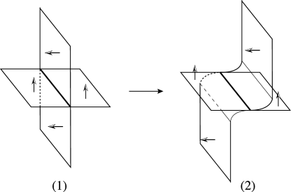
Figure 14. (1) Near the intersection of the oriented surfaces (Arrows shows the normal directions). (2) Modification near the intersection which agrees with the orientations of two surfaces.

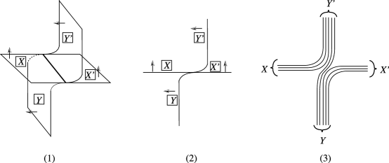
Figure 15. (1) Branch equation $X+Y=Y^{\prime}+X^{\prime}$. (2) Side view of (1) in this figure. (3) Side view of the surface induced by the branch equation. (In this case $X=X^{\prime}=3$, $Y=Y^{\prime}=5$.)

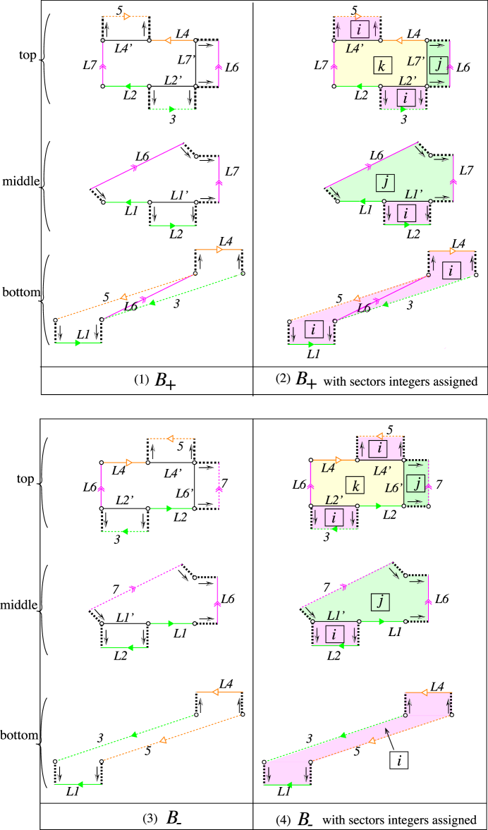
Figure 16. (1) Three pieces for building $\mathcal{B}_{+}$. (2) Assignment of sectors of $\mathcal{B}_{+}$. (3) Three pieces for building $\mathcal{B}_{-}$. (4) Assignment of sectors of $\mathcal{B}_{-}$. The types of arrows (red, green, yellow) are compatible with the ones illustrated in Figure 12.

Lemma 3.5.

The surface $S_{(i,j,k)_{\pm}}$ is the minimal representative of the fibered class $(i,j,k)_{\pm}$.

Proof.

By definition, $\Delta_{\pm}$ is a convex hull in $\Delta$ containing $\kappa_{\pm}$ ($\kappa_{+}=[1,1]$, $\kappa_{-}=[0,0]$), $\beta=[0,1]$, $\tfrac{\alpha+\beta}{2}=[\tfrac{1}{2},\tfrac{1}{2}]$, see Figure 5(3). The fibered class $(i,j,k)_{\pm}$ is in the cone over $\Delta_{\pm}$, and the surface $S_{(i,j,k)_{\pm}}$ is built from $\widehat{S}_{(i,j,k)_{\pm}}$ (which is the union of parallel copies of the minimal representatives $F_{\kappa_{\pm}}$, $F_{\beta}$ and $F_{\alpha+\beta}$) by cut and past construction. Thus $S_{(i,j,k)_{\pm}}$ must be the minimal representative of $(i,j,k)_{\pm}$. ∎

Remark 3.6.

By Lemma 3.5, we write $F_{(i,j,k)_{\pm}}=S_{(i,j,k)_{\pm}}$, and $F_{(i,j,k)_{\pm}}$ becomes a fiber of the fibration associated to $(i,j,k)_{\pm}$. By Theorem 2.3, $F_{(i,j,k)_{\pm}}$ (up to isotopy) is transverse to the flow $\Phi_{\alpha+\beta}^{t}$. The first return map $\Phi_{(i,j,k)_{\pm}}:F_{(i,j,k)_{\pm}}\rightarrow F_{(i,j,k)_{\pm}}$ with respect to $\Phi_{\alpha+\beta}^{t}$ becomes the pseudo-Anosov monodromy of the fibration associated $(i,j,k)_{\pm}$.

3.4. Train tracks $\tau_{(i,j,k)_{\pm}}$

We note that the unstable foliation $\mathcal{F}_{\alpha+\beta}$ of $\Phi_{\alpha+\beta}$ is carried by $\tau_{\alpha+\beta}$. Let $\widehat{\mathcal{F}}$ be the suspension of $\mathcal{F}_{\alpha+\beta}$ by $\Phi_{\alpha+\beta}$ which is the $2$-dimensional foliation of ${\mathbb{T}}_{\phi_{\alpha+\beta}}$. We now construct the branched surfaces $\mathcal{B}_{\Delta_{\pm}}$, each of which carries $\widehat{\mathcal{F}}$. Let $\delta$ and $\epsilon$ be as in Section 3.3, that is $\delta$ and $\epsilon$ are constants such that $0<\delta<2\delta<1-\epsilon$. Hereafter we fix $\delta=\tfrac{1}{3}$. We choose two families $\{\tau_{t}^{+}\}_{0\leq t\leq 1}$ and $\{\tau_{t}^{-}\}_{0\leq t\leq 1}$ of train tracks with the following properties. (See Figure 17, in which the time $t$ increases along arrows.)

1. $\tau_{0}^{+}=\tau_{0}^{-}=\Phi_{\alpha+\beta}(\tau_{\alpha+\beta})$.

2. $\tau_{t}^{+}=\tau_{t}^{-}=\tau_{\alpha+\beta}$ for $1-\epsilon_{0}\leq t\leq 1$.

3. $\tau_{t}^{\pm}$ is obtained from $\tau_{s}^{\pm}$ by folding edges of $\tau_{s}^{\pm}$ for each $0\leq s<t\leq 1-\epsilon$, or $\tau_{t}^{\pm}$ is isotopic to $\tau_{s}^{\pm}$,

4. $\tau_{t}^{+}=\tau_{t}^{-}$ for $0\leq t\leq\frac{2}{3}$, and $\{\tau_{t}^{\pm}\}_{0\leq t\leq\frac{2}{3}}$ is given as in Figure 17(3),

5. $\{\tau_{t}^{+}\}_{\frac{2}{3}<t\leq 1-\epsilon}$ (resp. $\{\tau_{t}^{-}\}_{\frac{2}{3}<t\leq 1-\epsilon}$) is given as in Figure 17(1) (resp. (2)).

In Figure 17, $\sigma\xrightarrow[\mathrm{folding}]{}\tau$ (resp. $\sigma\xrightarrow[\mathrm{isotopy}]{}\tau$) means that $\tau$ is obtained from $\sigma$ by folding edges of $\sigma$, (resp. $\tau$ is isotopic to $\sigma$). Observe that non-loop edges of $\tau_{1/3}^{+}=\tau_{1/3}^{-}$ (resp. $\tau_{2/3}^{+}=\tau_{2/3}^{-}$) do not intersect with $V$ and $W$ (resp. with $U$), see Figure 17(4)(5). The branched surfaces $\mathcal{B}_{\Delta_{\pm}}\subset{\mathbb{T}}_{\phi_{\alpha+\beta}}$ are defined to be

(3.3) $$\mathcal{B}_{\Delta_{\pm}}=\bigcup_{0\leq t\leq 1}\tau_{t}^{\pm}\times\{t\}/\sim,$$

where $\sim$ identifies $(x,1)$ and $(\Phi_{\alpha+\beta}(x),0)$ for $x\in\tau_{\alpha+\beta}$.

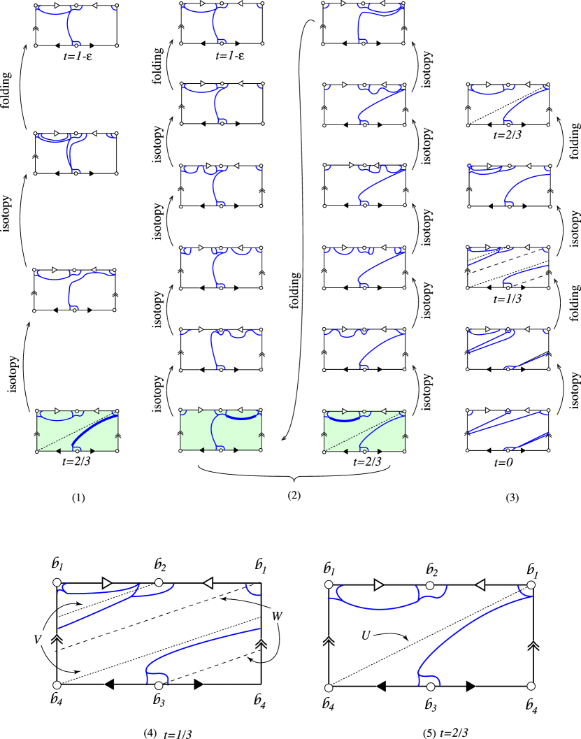
Figure 17. (Some of times $t$ are indicated near the puncture $\mathfrak{b}_{3}$.) (1) $\{\tau_{t}^{+}\}_{2/3<t\leq 1-\epsilon}$. (2) $\{\tau_{t}^{-}\}_{2/3<t\leq 1-\epsilon}$. (3) $\{\tau_{t}^{\pm}\}_{0\leq t\leq 2/3}$. (4) $\tau_{1/3}^{+}=\tau_{1/3}^{-}$. (5) $\tau_{2/3}^{+}=\tau_{2/3}^{-}$.

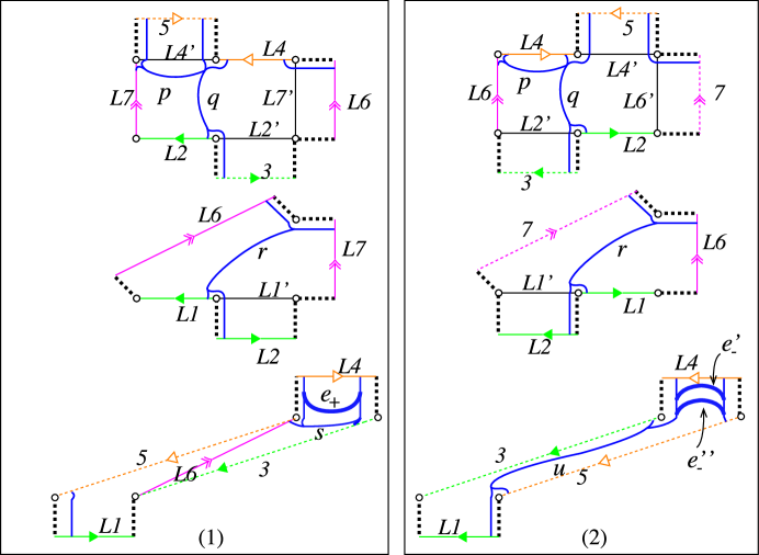
Figure 18. (1) $\mathcal{B}_{+}\cap\mathcal{B}_{\Delta_{+}}$. (2) $\mathcal{B}_{-}\cap\mathcal{B}_{\Delta_{-}}$. (cf. Figure 16(1)(3).)

Remark 3.7.

The condition (5) above makes the difference between $\mathcal{B}_{\Delta_{+}}$ and $\mathcal{B}_{\Delta_{-}}$. The conditions (1)–(4) (without (5)) allow us to construct a branched surface which carries $\widehat{\mathcal{F}}$. The reason we require (5) is that it is easy to extract a train track on $F_{(i,j,k)_{\pm}}$ from the intersection $F_{(i,j,k)_{\pm}}\cap\mathcal{B}_{\Delta_{\pm}}$ with the extra condition (5), see Lemma 3.9(2).

Remark 3.8.

The following analysis is used in the proof of Lemma 3.9(2). It happens twice that an edge of some element in the subfamily $\{\tau_{t}^{-}\}_{1/3\leq t\leq 1-\epsilon}$ is passing through the segment $K$ through the isotopy, see Figure 17(2)(3). On the other hand, the same thing happens once in the subfamily $\{\tau_{t}^{+}\}_{1/3\leq t\leq 1-\epsilon}$, see Figure 17(1)(3). In the same figure, $4$-punctured disks containing the track tracks in question are colored, and edges of these train tracks in question are made thick.

Since $F_{(i,j,k)_{\pm}}$ (up to isotopy) is transverse to the flow $\Phi_{\alpha+\beta}^{t}$, we may assume that $F_{(i,j,k)_{\pm}}$ is transverse to $\mathcal{B}_{{\Delta}_{\pm}}$. We let

(3.4) $$\tau_{(i,j,k)_{\pm}}^{\prime}=F_{(i,j,k)_{\pm}}\cap\mathcal{B}_{{\Delta}_{\pm}}.$$

Lemma 3.9.

1. The unstable foliation $\mathcal{F}_{(i,j,k)_{\pm}}$ of the pseudo-Anosov $\Phi_{(i,j,k)_{\pm}}$ is carried by $\tau_{(i,j,k)_{\pm}}^{\prime}$.

2. Each component of $F_{(i,j,k)_{\pm}}\setminus\tau_{(i,j,k)_{\pm}}^{\prime}$ is either a bigon (a disk with $2$ cusps) or a once punctured disk (i.e, annulus) with $k$ cusps for some $k\geq 1$.

Proof.

(1) By Theorem 2.3, we have $\mathcal{F}_{(i,j,k)_{\pm}}=F_{(i,j,k)_{\pm}}\cap\widehat{\mathcal{F}}$. Moreover its suspension $\widehat{\mathcal{F}}_{(i,j,k)_{\pm}}$ by $\Phi_{(i,j,k)_{\pm}}$ is isotopic to $\widehat{\mathcal{F}}$, see [28, Corollary 3.2]. Since $\widehat{\mathcal{F}}$ is carried by the branched surface $\mathcal{B}_{\Delta_{\pm}}$, so is $\widehat{\mathcal{F}}_{(i,j,k)_{\pm}}$. This implies that $\mathcal{F}_{(i,j,k)_{\pm}}$ is carried by $\tau_{(i,j,k)_{\pm}}^{\prime}=F_{(i,j,k)_{\pm}}\cap\mathcal{B}_{{\Delta}_{\pm}}$.

(2) We recall that the suitable branch equations on $\mathcal{B}_{\pm}$ induce $F_{(i,j,k)_{\pm}}$. Also recall that we need to insert some flowbands between the two segments with the same labeling to get the whole picture of $\mathcal{B}_{\pm}$. To view components of $F_{(i,j,k)_{\pm}}\setminus\tau_{(i,j,k)_{\pm}}^{\prime}$, let us consider $\mathcal{B}_{\pm}\cap\mathcal{B}_{\Delta_{\pm}}$ on $\mathcal{B}_{\pm}$ which is a $1$-branched manifold. We recall the definition of $\widehat{\mathcal{B}}_{\pm}$, see (3.1) and (3.2). The constant $\delta$ is chosen to be $\tfrac{1}{3}$ and we have the train tracks $\tau_{1-\epsilon}^{+}=\tau_{1-\epsilon}^{-}=\tau_{\alpha+\beta}$, $\tau_{2/3}^{+}=\tau_{2/3}^{-}$, $\tau_{1/3}^{+}=\tau_{1/3}^{-}$, see Figure 17. Then the ‘patterns’ in Figure 18(1)(2) are obtained from $\mathcal{B}_{\pm}\cap\mathcal{B}_{\Delta_{\pm}}$ after folding or splitting all edges which appear on the flowbands. In fact the thick edge $e_{+}$ in Figure 18(1) is the one (resp. thick edges $e_{-}^{\prime}$ and $e_{-}^{\prime\prime}$ in Figure 18(2) are the ones) by folding some edge (resp. by splitting some edges) which appear(s) on the flowband between the segments with the labeling $L4$, see also Remark 3.8. Then we reconstruct the fibers $F_{(i,j,k)_{\pm}}$ obtained from the suitable branch equations on $\mathcal{B}_{\pm}$ with the ‘patterns’ in Figure 18(1)(2) . That we get is $\tau_{(i,j,k)_{\pm}}^{\prime}$ (up to folding and splitting the edges) on $F_{(i,j,k)_{\pm}}$. Each edge of $\tau_{(i,j,k)_{\pm}}^{\prime}$ originates in some edge of the branched $1$-manifold $\mathcal{B}_{\pm}\cap\mathcal{B}_{\Delta_{\pm}}$. We denote some of the edges of $\mathcal{B}_{+}\cap\mathcal{B}_{\Delta_{+}}$ (resp. $\mathcal{B}_{-}\cap\mathcal{B}_{\Delta_{-}}$) by $p$, $q$, $r$, $s$ (resp. $p$, $q$, $r$, $u$) as in Figure 18(1) (resp. (2)).

We can fold all edges of $\tau_{(i,j,k)_{+}}^{\prime}$ (resp. $\tau_{(i,j,k)_{-}}^{\prime}$) which originate in $e_{+}$ (resp. $e_{-}^{\prime}$ or $e_{-}^{\prime\prime}$) into some edges. This means that these edges lie on the boundaries of some components of $F_{(i,j,k)_{\pm}}\setminus\tau_{(i,j,k)_{\pm}}^{\prime}$ that are bigons. We fold all these edges as much as possible (i.e, collapse bigons), and we consider complementary regions of the resulting $1$-branched manifold. The combinatorics from Figures 16(2)(4) and 18 tell us that each component of the resulting $1$-branched manifold is a once punctured disk with $k$ cusps for some $k\geq 1$. ∎

Let $\tau_{(i,j,k)_{\pm}}$ be the branched $1$-manifold obtained from $\tau_{(i,j,k)_{\pm}}^{\prime}$ by collapsing all bigons of $\tau_{(i,j,k)_{\pm}}^{\prime}$. By Lemma 3.9, we immediately have:

Lemma 3.10.

$\tau_{(i,j,k)_{\pm}}$ is a train track on $F_{(i,j,k)_{\pm}}$ which carries $\mathcal{F}_{(i,j,k)_{\pm}}$.

3.5. Monodromies $\Phi_{(i,j,k)_{\pm}}:F_{(i,j,k)_{\pm}}\rightarrow F_{(i,j,k)_{\pm}}$ of the fibrations associated to $(i,j,k)_{\pm}$

First of all, we represent fibers $F_{(i,j,k)_{\pm}}$ more simpler as follows. We shrink each flowband of $F_{(i,j,k)_{\pm}}$ as much as possible along flow lines into some edge. (Note that this operation does not change the topological type of fibers.) Said differently, we simplify the branched surfaces $\mathcal{B}_{\pm}$ as follows. Shrink each flowband of the three pieces, see Figure 16(1) (resp. (3)), as much as possible along flow lines into some edge. Then the branch equations on $\mathcal{B}_{\pm}$ induces the one on such a simplified branched surface, from which one gets a surface in question which is homeomorphic to $F_{(i,j,k)_{\pm}}$.

After shrinking flowbands, the resulting three pieces (the bottom, middle, top pieces) are:

1. $\kappa_{+}$-patch: the two acute-angled triangles sharing vertices $\mathfrak{b}_{1}$ and $\mathfrak{b}_{4}$
   (resp. $\kappa_{-}$-patch: the parallelogram),

2. $\beta$-patch: the right-angled triangle, and

3. $\alpha+\beta$-patch: the rectangle.

We call these pieces (1) $\kappa_{+}$-patch (resp. $\kappa_{-}$-patch ), (2) $\beta$-patch and (3) $\alpha+\beta$-patch. See Figure 19(1) (resp. Figure 20(1)) for three kinds of patches. We often draw pairs of the two acute-angled triangles for the $\kappa_{+}$-patch separately as in Figure 19(1), but they should share the two vertices $\mathfrak{b}_{1}$ and $\mathfrak{b}_{4}$ (cf. Figure 11(3)). We can get the simplified fibers $F_{(i,j,k)_{+}}$ (resp. $F_{(i,j,k)_{-}}$) from $i$ parallel copies of $\kappa_{+}$-patches (resp. $\kappa_{-}$-patches), $j$ parallel copies of $\beta$-patches and $k$ parallel copies of $\alpha+\beta$-patches under suitable identifications of the boundaries of patches.

If we have $j$ parallel copies of the same kind of patches, say $\beta$-patches, ${\mathbb{P}}_{\beta}^{1},\cdots,{\mathbb{P}}_{\beta}^{j}$, we have ${\mathbb{P}}_{\beta}^{\ell}\subset F_{\alpha+\beta}^{n_{\ell}}$ for some $0<n_{\ell}<1$, where $\ell\in\{1,\cdots,j\}$. For the notation of $F_{\alpha+\beta}^{n_{\ell}}$, see the end of Section 3.2. If $0<n_{1}<\cdots<n_{j-1}<n_{j}<1$, then we call the $\beta$-patch ${\mathbb{P}}_{\beta}^{1}$ the bottom ($\beta$-)patch, and call ${\mathbb{P}}_{\beta}^{j}$ the top ($\beta$-)patch. Other $\beta$-patches are called the middle ($\beta$-)patches. We define the top, middle, bottom for other patches similarly. We color each top of the three kinds of patches, see Figure 19(1)(left column), Figure 20(1)(left column). Here we label $E^{\prime}$ for the top $\beta$-patch, and label $F^{\prime}$ and $G^{\prime}$ (resp. $F^{\prime}$) for the top $\kappa_{+}$-patch (resp. $\kappa_{-}$-patch) in the same figure. We label $A^{\prime}$, $B^{\prime}$, $C^{\prime}$ and $D^{\prime}$ for isosceles right-angled triangles which lies on the top $\alpha+\beta$-patch.

The patches needed for building $F_{(i,j,k)_{\pm}}$ for the non-degenerate class $(i,j,k)_{\pm}$ are given as in the same figure. We can think three kinds of patches are in the cylinder $\varSigma_{0,4}\times(0,1)\subset{\mathbb{T}}_{\phi_{\alpha+\beta}}$. We have the flow direction in the cylinder from the ‘bottom’ $\varSigma_{0,4}\times\{0\}$ to the ‘top’ $\varSigma_{0,4}\times\{1\}$. The types of arrows (red, green, yellow) in the figure are compatible with the ones illustrated in Figures 12 and 16. Among the patches with the same kind ($\kappa_{\pm}$-patches, $\beta$-patches or $\alpha+\beta$-patches), the way to label parallel segments with the same kind of arrow is that the number for the labeling increases (cyclically) along the flow direction. We often omit to label segments which lie on the middle patches. To get the fiber $F_{(i,j,k)_{\pm}}$, we identify the two segments with the same kind of arrow and with the same labeling (same number) by using the flow $\Phi_{\alpha+\beta}^{t}$. In the right column of (1) in the same figure, the labeling of segments on patches are the same as the one given in the left column.

Let us turn to construct $\Phi_{(i,j,k)_{\pm}}:F_{(i,j,k)_{\pm}}\rightarrow F_{(i,j,k)_{\pm}}$ explicitly. It is enough to describe where each patch maps to. Since the desired monodromy $\Phi_{(i,j,k)_{\pm}}$ is the first return map on $F_{(i,j,k)_{\pm}}$ with respect to $\Phi_{\alpha+\beta}^{t}$, we see the followings. All patches but the top of each kind of patches map to the next above patch (of the same kind) along the flow direction. Thus the monodromy $\Phi_{(i,j,k)_{\pm}}$ restricted to these patches is just a shift map. On the other hand, each top patches map to some bottom patches (possibly with different kinds), see Figure 19(1) for $\Phi_{(i,j,k)_{+}}$ and see Figure 20(1) for $\Phi_{(i,j,k)_{-}}$, where $A,B,\cdots$ are the images of $A^{\prime},B^{\prime},\cdots$ under $\Phi_{(i,j,k)_{\pm}}$. More precisely, we can get the image of the top $\beta$-patch under $\Phi_{(i,j,k)_{\pm}}$ when we push the fiber $F_{(i,j,k)_{\pm}}$ along the flow direction and see how this top patch hits to the bottom $\alpha+\beta$-patch. Similarly, one can get the image of the top $\kappa_{+}$-patch (resp. top $\kappa_{-}$-patch) under $\Phi_{(i,j,k)_{+}}$ (resp. $\Phi_{(i,j,k)_{-}}$) if we see how this top patch hit to the both bottom $\beta$-patch and bottom $\alpha+\beta$-patch. To get the images of the isosceles right-angled triangles $A^{\prime}$, $B^{\prime}$, $C^{\prime}$ and $D^{\prime}$ which lies on the top $\alpha+\beta$-patch, we first consider the acute-angled triangles $A$, $B$, $C$ and $D$ which lie on $\varSigma_{0,4}\times\{0\}$ as in Figure 8(right). Then investigate how these acute-angled triangles hit bottoms patches, when we push them along the flow direction.

The monodromies of the fibrations associated to the degenerated classes can be constructed similarly. As an example, we deal with the degenerated classes $a=(j,k)_{0}$’s, see Figure 21.

Remark 3.11.

Suppose that $(j,k)_{0}$ is primitive (i.e, $\gcd(j,k)=1$). Then the fiber $F_{(j,k)_{0}}$ is connected, and it has genus $0$, see [18]. Many pseudo-Anosovs with small dilatations defined on the surfaces of genus $0$ are contained in the family of fibered classes $(j,k)_{0}$’s, see Examples 4.6, 4.7 and [18, Section 4.1]. By using the Artin generators of the braid groups, the words which represent $\phi_{(j,k)_{0}}$’s are given in [18, Theorem 3.4]. They are quite simple words.

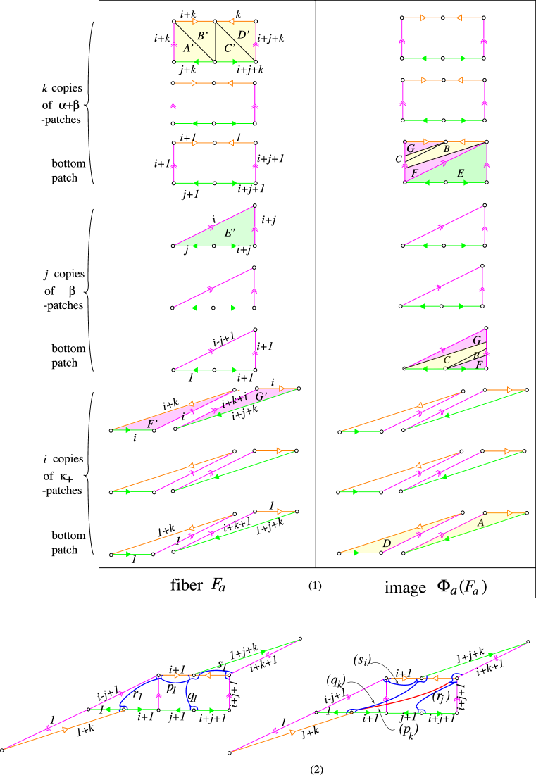
Figure 19. Labeling of segments in the right column of (1) is the same as the one in the left column. (1) $\Phi_{a}:F_{a}\rightarrow F_{a}$ for non-degenerate $a=(i,j,k)_{+}$. (2) (left) Bottom edges $s_{1}$, $r_{1}$, $p_{1}$ and $q_{1}$ which lie on three bottom patches. (right) Images of top edges $s_{i}$, $r_{j}$, $p_{k}$ and $q_{k}$ under $\Phi_{a}$ which lie on three bottom patches. We denote by $(s_{i})$ etc., the image $\Phi_{a}(s_{i})$ etc.

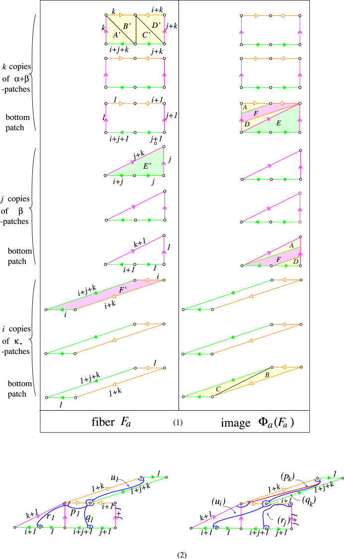
Figure 20. (1) $\Phi_{a}:F_{a}\rightarrow F_{a}$ for non-degenerate $a=(i,j,k)_{-}$. (2) (left) Bottom edges $u_{1}$, $r_{1}$, $p_{1}$ and $q_{1}$ which lie on three bottom patches. (right) Images of top edges $u_{i}$, $r_{j}$, $p_{k}$ and $q_{k}$ under $\Phi_{a}$ which lie on three bottom patches.

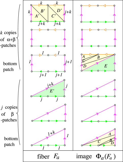
Figure 21. $\Phi_{a}:F_{a}\rightarrow F_{a}$ for degenerate $a=(j,k)_{0}$.

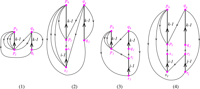
Figure 22. $\Gamma_{a}$ for $a=(i,j,k)_{+}$. (1)(2)(3) degenerate cases. (4) non-degenerate case. (1) $a=(0,k)_{0}$ with $k>0$. (2) $a=(i,0,k)_{+}$ with $i,k>0$. (3) $a=(j,k)_{0}$ with $j,k>0$. (4) $a=(i,j,k)_{+}$ with $i,j,k>0$.

Figure 23. $\Gamma_{a}$ for $a=(i,j,k)_{-}$. (1)(3) degenerate cases. (2)(4) non-generate cases. (1) $a=(i,0,k)_{-}$ with $0<i<k$. (2) $a=(i,j,k)_{-}$ with $0<i<k$. (3) $a=(i,0,k)_{-}$ with $i\geq k>0$. (4) $a=(i,j,k)_{-}$ with $i\geq k>0$. For (3)(4), $\ell\geq 1$ is an integer such that $0\leq i-k\ell\leq k-1$.

3.6. Train track representatives $\mathfrak{p}_{(i,j,k)_{\pm}}:\tau_{(i,j,k)_{\pm}}\rightarrow\tau_{(i,j,k)_{\pm}}$ of $\phi_{(i,j,k)_{\pm}}$

In the following lemma, we use the metrized, directed graph $\Gamma_{(i,j,k)_{\pm}}$ given in Figures 22 and 23, where each edge with no labeling means that its length is equal to $1$, and all edges with labeling are made thick in the figures.

Lemma 3.12.

1. The train track $\tau_{(i,j,k)_{\pm}}$ is invariant under $\phi_{(i,j,k)_{\pm}}=[\Phi_{(i,j,k)_{\pm}}]$. If we let $\mathfrak{p}_{(i,j,k)_{\pm}}:\tau_{(i,j,k)_{\pm}}\rightarrow\tau_{(i,j,k)_{\pm}}$ be the train track representative of $\phi_{(i,j,k)_{\pm}}$, then its incidence matrix is Perron-Frobenius.

2. The directed graph $\Gamma_{(i,j,k)_{\pm}}$ is the one induced by $\mathfrak{p}_{(i,j,k)_{\pm}}:\tau_{(i,j,k)_{\pm}}\rightarrow\tau_{(i,j,k)_{\pm}}$,

Once we prove that $\tau_{(i,j,k)_{\pm}}$ is invariant under $\phi_{(i,j,k)_{\pm}}$, the claim that the incidence matrix of $\phi_{(i,j,k)_{\pm}}$ is Perron-Frobenius follows from Theorem 2.1.

Proof of Lemma 3.12.

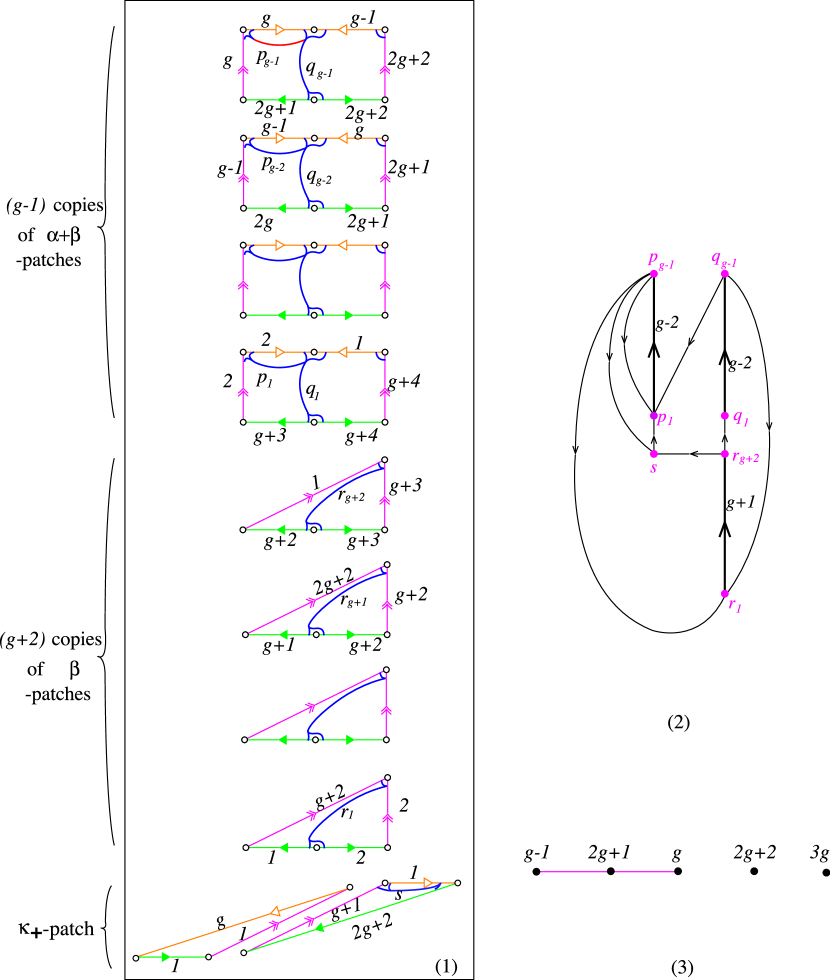
Figure 30. Example 4.2. (1) $\tau_{a_{g}}\subset F_{a_{g}}$ (2) $\Gamma_{a_{g}}$ (3) $G_{a_{g}}$ for $a_{g}=(1,g+2,g-1)_{+}$.

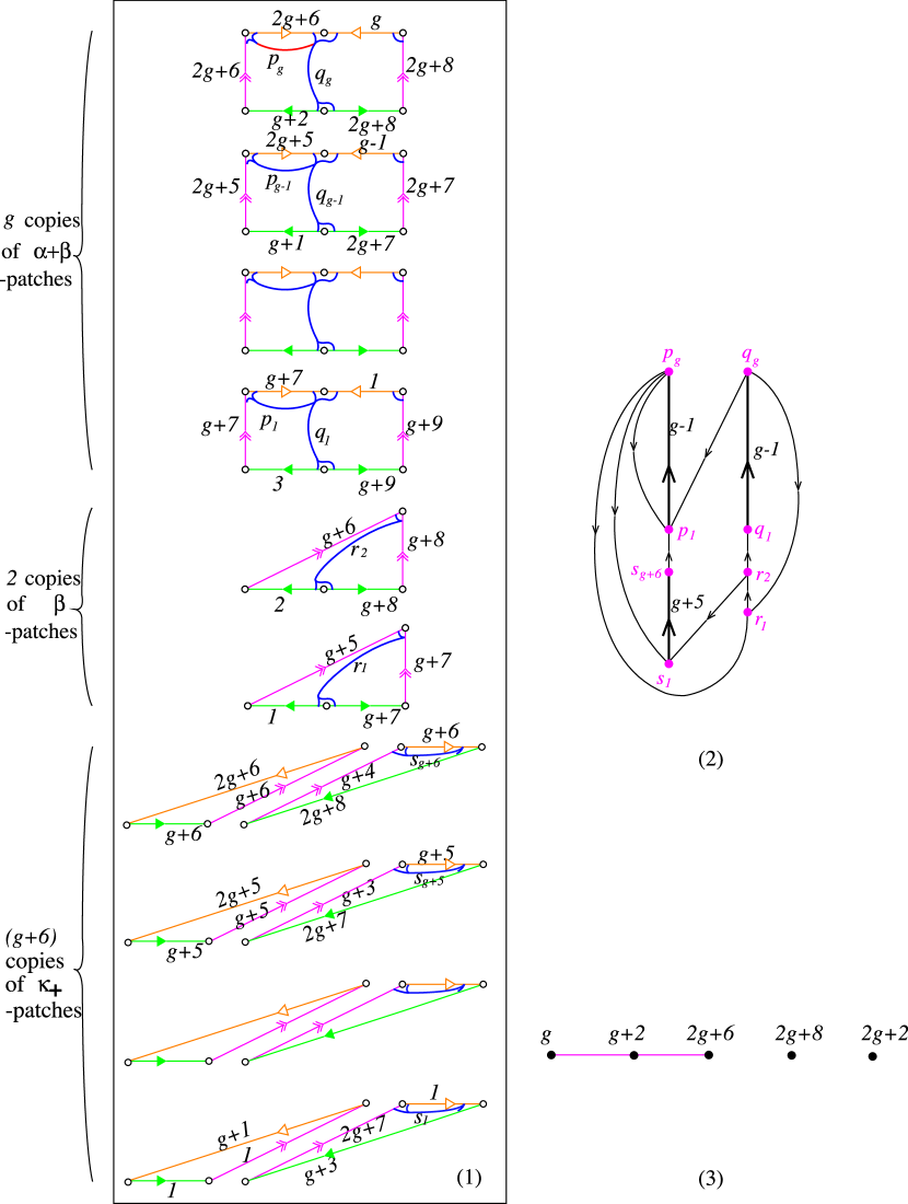
Figure 31. Example 4.3. (1) $\tau_{a_{g}}\subset F_{a_{g}}$ (2) $\Gamma_{a_{g}}$ (3) $G_{a_{g}}$ for $a_{g}=(g+6,2,g)_{+}$.

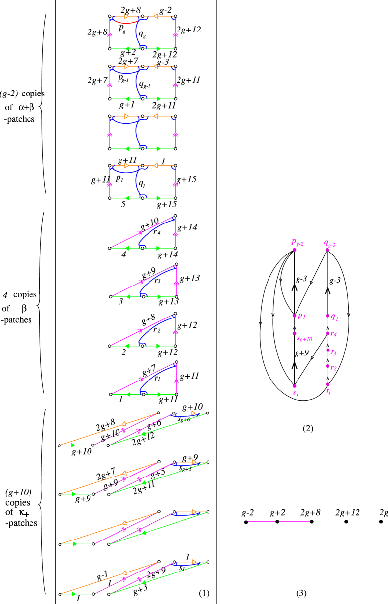
Figure 32. Example 4.4. (1) $\tau_{a_{g}}\subset F_{a_{g}}$ (2) $\Gamma_{a_{g}}$ (3) $G_{a_{g}}$ for $a_{g}=(g+10,4,g-2)_{+}$.

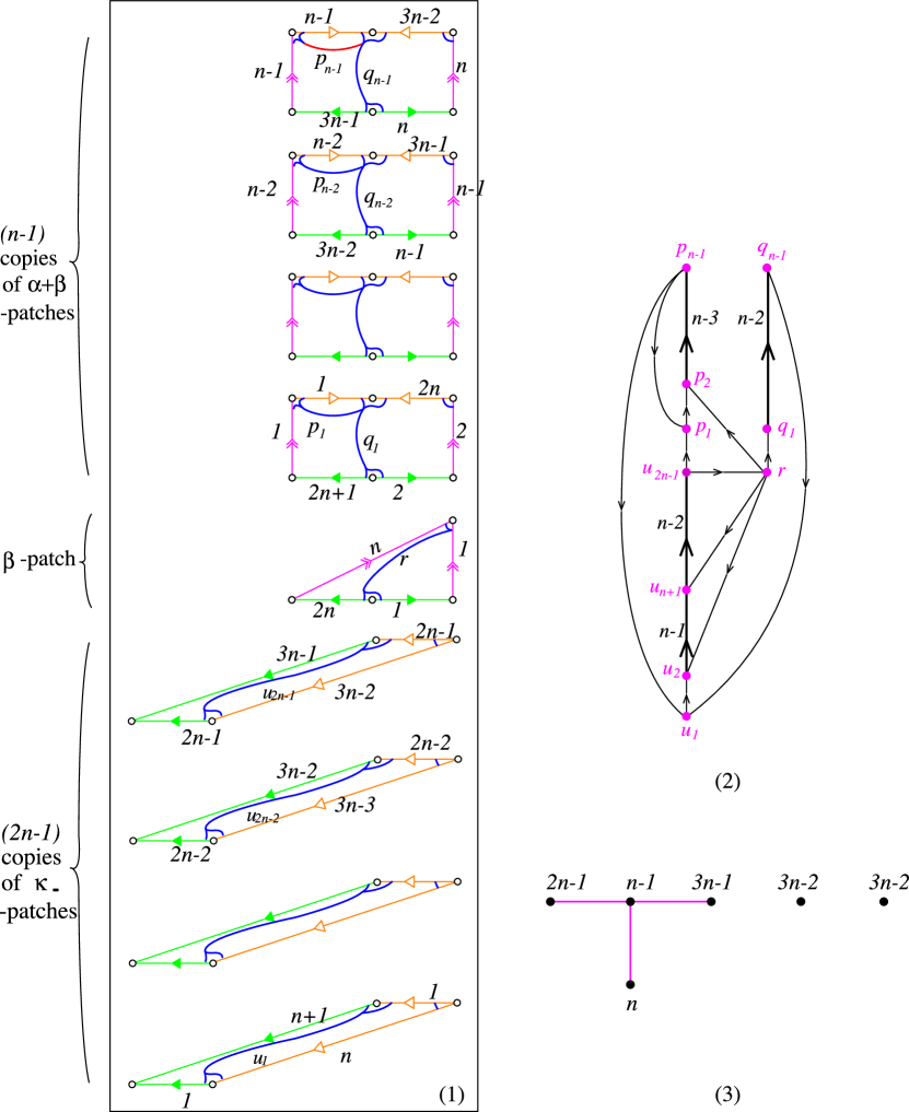
Figure 33. Example 4.5. (1) $\tau_{a_{n}}\subset F_{a_{n}}$ (2) $\Gamma_{a_{n}}$ (3) $G_{a_{n}}$ for $a_{n}=(2n-1,1,n-1)_{-}$.

By construction of $\tau_{(i,j,k)_{\pm}}$, each edge of $\tau_{(i,j,k)_{\pm}}$ originates in some edge of the intersection $\mathcal{B}_{\pm}\cap\mathcal{B}_{\Delta_{\pm}}$ (see Figure 18). We only label edges of $\tau_{(i,j,k)_{+}}$ (resp. $\tau_{(i,j,k)_{-}}$) which originate in the edges $p,q,r$ and $s$ (resp. $p,q,r$ and $u$), since it turns out that the images of other edges under $\Phi_{(i,j,k)_{\pm}}$ are eventually periodic up to isotopy. We first explain the way to label the edges of $\tau_{(i,j,k)_{\pm}}$, which is similar to the one to label segments of patches given in Section 3.5. We label parallel edges of $\tau_{(i,j,k)_{\pm}}$ (which originate in the same edge of $\mathcal{B}_{\pm}\cap\mathcal{B}_{\Delta_{\pm}}$) so that the number for the labeling increases along the flow direction. For example, see Figures 30–36.

We only prove the claims (1) and (2) for non-degenerate classes $(i,j,k)_{\pm}$. (The proofs for degenerate classes are similar.) Let us describe the image of an edges $e$ with labeling under $\Phi_{(i,j,k)_{\pm}}$. Such an edge $e$ lies on some patch for building $F_{(i,j,k)_{\pm}}$. Suppose that $e$ lies on a patch, say ${\mathbb{P}}_{e}$ which is not a top patch. Then $e$ maps (under $\Phi_{(i,j,k)_{\pm}}$) to the next above edge $e^{\prime}$ which lies on the same kind of patch ${\mathbb{P}}_{e^{\prime}}$ as ${\mathbb{P}}_{e}$. Clearly, $e$ and $e^{\prime}$ originate in the same edge of $\mathcal{B}_{\pm}\cap\mathcal{B}_{\Delta_{\pm}}$. Suppose that an edge $e_{\mathrm{top}}$ of $\tau_{(i,j,k)_{\pm}}$ lies on some top patch. We call $e_{\mathrm{top}}$ the top edge. If an edge $e_{\mathrm{bot}}$ of $\tau_{(i,j,k)_{\pm}}$ lies on some bottom patch, then we call $e_{\mathrm{bot}}$ the bottom edge.

We first consider the non-degenerate class $(i,j,k)_{+}$. Let us consider the images $\Phi_{(i,j,k)_{+}}(e_{\mathrm{top}})$’s for all top edges $e_{\mathrm{top}}$’s. Then we can put $\Phi_{(i,j,k)_{+}}(e_{\mathrm{top}})$’s in the tie neighborhood of $\tau_{(i,j,k)_{+}}$ which are transverse to the ties up to isotopy, where the support of the isotopy can be taken on the neighborhood of the three bottom patches, see Figure 19(2). Thus $\tau_{(i,j,k)_{+}}$ is invariant under $\phi_{(i,j,k)_{+}}$. In fact we can get the edge path $\mathfrak{p}_{(i,j,k)_{+}}(e_{\mathrm{top}})$ from Figure 19(2): The left of (2) of the same figure illustrates the union of all bottom edges of $\tau_{(i,j,k)_{+}}$ which lie on the union of all bottom patches. The right of (2) of the same figure shows the image of all top edges under $\Phi_{(i,j,k)_{+}}$. One can find from the right in (2) of the same figure that $\mathfrak{p}_{(i,j,k)_{+}}(p_{k})$ and $\mathfrak{p}_{(i,j,k)_{+}}(q_{k})$ pass through the three edges $r_{1}$, $p_{1}$, $s_{1}$, and the two edges $r_{1}$, $p_{1}$ respectively. The edge path $\mathfrak{p}_{(i,j,k)_{+}}(r_{j})$ passes through the two edges $q_{1}$, $s_{1}$.

Note that by Remark 3.2, we see that edges of $\tau_{(i,j,k)_{+}}$ which originate in the edges $p,q,r$ and $s$ are real edges for $\mathfrak{p}_{(i,j,k)_{+}}$. Others are infinitesimal edges. We explain a structure of the directed graph in Figure 22(4). When $e$ is an edge with some label (which are made thick in the figure), then the end points of $e$ are the vertices having the same origin ($p$, $q$, $r$ or $s$) on $\mathcal{B}_{+}$. Suppose that $e$ is an edge whose length equals $k-1$, and suppose that $e$ has end points $p_{1}$ and $p_{k}$ having the same origin $p$. Then the edge $e$ with labeling $k-1$ corresponds to the following edge path with length $k-1$:

$$p_{1}\rightarrow p_{2}\rightarrow\cdots\rightarrow p_{k-1}\rightarrow p_{k}.$$

In particular all vertices between $p_{1}$ and $p_{k}$ have the same origin $p$ on $\mathcal{B}_{+}$. Putting these things together, we can check that metrized, directed graph $\Gamma_{(i,j,k)_{+}}$ in Figure 22(4) is the one induced by $\mathfrak{p}_{(i,j,k)_{+}}:\tau_{(i,j,k)_{+}}\rightarrow\tau_{(i,j,k)_{+}}$.

We turn to the non-degenerate class $(i,j,k)_{-}$. In the same manner as in the class $(i,j,k)_{+}$, we can see that $\tau_{(i,j,k)_{-}}$ is invariant under $\phi_{(i,j,k)_{-}}$. The edges of $\tau_{(i,j,k)_{-}}$ which originate in the edges $p,q,r$ and $u$ are real edges for the train track representative $\mathfrak{p}_{(i,j,k)_{-}}$ of $\phi_{(i,j,k)_{-}}$. Others are infinitesimal edges. A hint to obtain $\mathfrak{p}_{(i,j,k)_{-}}(e_{\mathrm{top}})$ is given in Figure 20(2). The left of (2) in the same figure illustrates the union of all bottom edges of $\tau_{(i,j,k)_{-}}$ which lie on the union of all bottom patches. The right of (2) in the same figure shows the image of all top edges under $\Phi_{(i,j,k)_{-}}$. The images under $\mathfrak{p}_{(i,j,k)_{-}}$ of all top edges but $r_{j}$ are edge paths written by bottom edges. For example, $\mathfrak{p}_{(i,j,k)_{-}}(u_{i})$ is an edge path which passes through $r_{1}$ and $p_{1}$. On the other hand, to put $\Phi_{(i,j,k)_{-}}(r_{j})$ in the tie neighborhood of $\tau_{(i,j,k)_{-}}$ one needs to make $\Phi_{(i,j,k)_{-}}(r_{j})$ (up to isotopy) across the segment $K$. An analysis to identify boundaries of patches for building $F_{(i,j,k)_{-}}$ enables us to get the image $\mathfrak{p}_{(i,j,k)_{-}}(r_{j})$. We can verify that the directed graph $\Gamma_{(i,j,k)_{-}}$ given in Figure 23(2) (resp. (4)) is the one induced by $\mathfrak{p}_{(i,j,k)_{-}}$ if $0<i<k$ (resp. $i\geq k>0$). The edge path $\mathfrak{p}_{(i,j,k)_{-}}(r_{j})$ has length $\ell+2$, where $\ell\geq 0$ is an integer such that $0\leq i-k\ell\leq k-1$. ∎

Remark 3.13.

Metrized and directed graphs $\Gamma_{(i,j,k)_{\pm}}$ for non-degenerate classes can recover ones for degenerate classes. See Figures 18(1)(2)(3) and 22(1)(3). To see this, consider $\Gamma_{(i,j,k)_{+}}$ for the non-degenerate class $(i,j,k)_{+}$. We have the edge $p_{k}\to s_{1}$ and the edge path from $s_{1}$ to $p_{1}$ for $\Gamma_{(i,j,k)_{+}}$, see Figure 22(4). Connecting these edge paths, we have the edge path from $p_{k}$ to $p_{1}$ with length $>1$, see Figure 22(4). This determines the edge $p_{k}\to p_{1}$ with length $1$ in the degenerate class $(0,j,k)_{+}=(j,k)_{0}$ by ‘eliminating’ vertices $s_{1},\cdots,s_{i}$, see Figure 22(3). Another example is this. We have the edge $r_{j}\to s_{1}$ and the edge path from $s_{1}$ to $p_{1}$ for the non-degenerate class $(i,j,k)_{+}$, see Figure 22(4). They determine the edge $r_{j}\to p_{1}$ with length $1$ for the degenerate class $(0,j,k)_{+}=(j,k)_{0}$, see Figure 22(3).

3.7. Curve complexes $G_{(i,j,k)_{\pm}}$ and their clique polynomials $Q_{(i,j,k)_{\pm}}(t)$

We define some graphs. Let $K_{m,n}$ denote the complete bipartite graph with $m$ and $n$ vertices. We denote by $K_{m,n}^{**}$, the disjoint union of $K_{m,n}$ and the graph with two vertices and with no edges.

The metrized, directed graphs $\Gamma_{(i,j,k)_{+}}$’s and $\Gamma_{(i,j,k)_{-}}$’s were given in Section 3.6. Here we exhibit their curve complexes $G_{(i,j,k)_{+}}$’s in Figure 24 and $G_{(i,j,k)_{-}}$’s in Figure 25. In the next proposition, we give the clique polynomial $Q_{(i,j,k)_{\pm}}$ for the computation of $\lambda_{(i,j,k)_{\pm}}$. We find that it is equal to the polynomial $f_{(i,j,k)_{\pm}}(t)$ in Lemma 2.7(1).

Proposition 3.14.

The clique polynomial $Q_{(i,j,k)_{\pm}}(t)$ of the curve complex $G_{(i,j,k)_{\pm}}$ is the following reciprocal polynomial

$$Q_{(i,j,k)_{\pm}}(t)=1-(t^{k}+t^{i+k}+t^{j+k}+t^{i+j+k})+t^{i+j+2k}.$$

In particular, the dilatation $\lambda_{(i,j,k)_{+}}=\lambda_{(i,j,k)_{-}}$ is the largest root of $Q_{(i,j,k)_{+}}(t)=Q_{(i,j,k)_{-}}(t)$.

Proof.

It is straightforward to compute the clique polynomial $Q_{(i,j,k)_{\pm}}(t)$. The dilatation $\lambda_{(i,j,k)_{\pm}}$ equals the growth rate of $\Gamma_{(i,j,k)_{\pm}}$. By Theorem 2.5, $\tfrac{1}{\lambda_{(i,j,k)_{\pm}}}$ is the smallest root of $Q_{(i,j,k)_{\pm}}(t)$. Note that $Q_{(i,j,k)_{\pm}}(t)$ is a reciprocal polynomial, i.e, $Q_{(i,j,k)_{\pm}}(t)=t^{i+j+2k}Q_{(i,j,k)_{\pm}}(t^{-1})$. Thus the largest root of $Q_{(i,j,k)_{\pm}}(t)$ equals $\lambda_{(i,j,k)_{\pm}}$. ∎

Figure 24. $G_{a}$ for $a=(i,j,k)_{+}$. (1) $G_{a}=K_{1,3}^{**}$ if $a=(i,0,k)_{+}$ including the case $i=0$ and $k>0$, see Figure 22(1)(2). (2) $G_{a}=K_{1,2}^{**}$ if $a=(i,j,k)_{+}$ including the case $i=0$, $j>0$ and $k>0$, see Figure 22(3)(4).

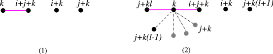
Figure 25. $G_{a}$ for $a=(i,j,k)_{-}$. (1) $G_{a}=K_{1,1}^{**}$ if $a=(i,j,k)_{-}$ with $0<i<k$ including the case $j=0$, see Figure 23(1)(2). (2) $G_{a}=K_{1,\ell+1}^{**}$ if $a=(i,j,k)_{-}$ with $i\geq k>0$ including the case $j=0$, see Figure 23(3)(4). Here $\ell\geq 1$ is an integer such that $0\leq i-k\ell\leq k-1$. The weights of $\ell+1$ vertices of the subgraph $K_{1,\ell+1}$ surrounding the centered vertex are given by $i+j+k$, $j+k,\cdots,j+k(\ell-1),j+k\ell$ clockwise.

Proof of Theorem 1.2.

Let $a$ be a fibered class of $N$. By a symmetry of Thurston norm ball $U_{N}$ and by Lemma 2.6(4), we may suppose that $a$ is of the form $(i,j,k)_{\pm}\in int(C_{\Delta})$. Suppose that $a=(0,0,1)_{\pm}=(0,1)_{0}$. In this case, we have constructed $\Phi_{a}:F_{a}\rightarrow F_{a}$ and $\mathfrak{p}_{a}:\tau_{a}\rightarrow\tau_{a}$ explicitly in Section 3.1.

Let us consider other fibered classes $a=(i,j,k)_{\pm}$’s. The explicit construction of the monodromy $\Phi_{a}:F_{a}\rightarrow F_{a}$ of the fibration associated to $a$ is given in Section 3.5. If $a$ is primitive, then the explicit construction of the desired train track representative $\mathfrak{p}_{a}:\tau_{a}\rightarrow\tau_{a}$ of $\phi_{a}$ together with the induced directed graph $\Gamma_{a}$ of $\mathfrak{p}_{a}$ (Figures 22 and 23) is given in Section 3.6. ∎

4. A catalogue of small dilatation pseudo-Anosovs

4.1. Fibered classes of Dehn fillings $N(r)$

Recall that $T_{\beta}$ (resp. $T_{\alpha}$, $T_{\gamma}$) is a torus which is the boundary of a regular neighborhood of the component $K_{2}$ (resp. $K_{1}$, $K_{3}$) of the $3$ chain link $\mathcal{C}_{3}$. Recall that $N(r)$ is the manifold obtained from $N$ by Dehn filling the cusp along the slope $r\in{\mathbb{Q}}\cup\{\infty\}$. It is known by [26] that $N(r)$ is hyperbolic unless $r\in\{\infty,-3,-2,-1,0\}$. The manifolds $N(\tfrac{3}{-2})$ and $N(\tfrac{1}{-2})$ are the exterior of the Whitehead sister link (i.e, $(-2,3,8)$-pretzel link) and the exterior of the $3$-braided link $\mathrm{br}(\sigma_{1}^{-1}\sigma_{2})$ (or $6_{2}^{2}$ link in Rolfsen’s table) respectively. Also $N(1)$ is the exterior of the Whitehead link (see [26] for example). These Dehn fillings $N(\tfrac{3}{-2})$, $N(\tfrac{1}{-2})$ and $N(1)$ play an important rule to study pseudo-Anosovs with small dilatations (see [17]), which we recall quickly in Section 4.3.

First of all, we consider the relation of fibered classes between $N$ and Dehn fillings $N(r)$. We suppose that $N(r)$ is the manifold obtained from $N$ by Dehn filling the cusp specified by $T_{\beta}$ along the slope $r$. By using Lemma 2.6(2) (which says that the boundary slope of $\partial_{\beta}F_{a}$ equals $\tfrac{z+x}{-y}$), we have the following: There exists a natural injection

$$\iota_{\beta}:H_{2}(N(r),\partial N(r))\rightarrow H_{2}(N,\partial N)$$

whose image equals $S_{\beta}(r)$, where

$$S_{\beta}(r)=\{(x,y,z)\in H_{2}(N,\partial N)\ |\ -ry=z+x\},$$

see [17, Proposition 2.11]. We choose $r\in{\mathbb{Q}}$ with $r\not\in\{-3,-2,-1,0\}$, and let $a\in S_{\beta}(r)=\mathrm{Im}\,\iota_{\beta}$ be a fibered class in $H_{2}(N,\partial N)$. Then $\overline{a}=\iota_{\beta}^{-1}(a)\in H_{2}(N(r),\partial N(r))$ is also a fibered class of $N(r)$. This is because the monodromy $\Phi_{a}:F_{a}\rightarrow F_{a}$ of the fibration on $N$ associated to $a$ extends to the monodromy $\overline{\Phi}_{a}$ of the fibration on $N(r)$ associated to $\overline{a}$ by capping each boundary component of $\partial_{\beta}F_{a}$ with the disk. If the (un)stable foliation $\mathcal{F}_{a}$ of $\Phi_{a}$ has a property such that each component of $\partial_{\beta}F_{a}$ has no $1$ prong, then $\mathcal{F}_{a}$ extends canonically to the (un)stable foliation $\overline{\mathcal{F}}_{a}$ of $\overline{\Phi}_{a}$, and hence $\overline{\Phi}_{a}$ becomes a pseudo-Anosov homeomorphism with the same dilatation as $\Phi_{a}$. We sometimes denote $N(r)$ by $N_{\beta}(r)$ when we need to specify the cusp which is filled. By using this notation, we may write $\overline{a}\in H_{2}(N_{\beta}(r),\partial N_{\beta}(r))$.

Similarly, when $N(r)$ is the manifold obtained from $N$ by Dehn filling the cusp specified by another torus $T_{\gamma}$ along the slope $r$, we have a natural injection,

$$\iota_{\gamma} :H_{2}(N(r),\partial N(r))\to H_{2}(N,\partial N)$$

whose image $\mathrm{Im}\,\iota_{\gamma}$ is given by

$$S_{\gamma}(r) =\{(x,y,z)\in H_{2}(N,\partial N)\,|\,-rz=x+y\}.$$

4.2. Concrete examples

In the following example, we consider some fibered classes $a$ and compute their dilatations $\lambda(a)$. We also exhibit $\tau_{a}\subset F_{a}$, its image $\Phi_{a}(\tau_{a})$ putting into the tie neighborhood $\mathcal{N}(\tau_{a})$ (so that it is transverse to the ties) and the directed graph $(\Gamma_{a},{\bf 1})$.

Example 4.1.

1. If $a=(1,4,1)_{+}=(2,6,1)$, then $\lambda(a)\approx 1.7220$ is the largest root of

   $$Q_{(1,4,1)_{+}}(t)=f_{(2,6,1)}(t)=(t^{3}+1)(t^{4}-t^{3}-t^{2}-t+1).$$

   By Lemma 2.6(3), the topological type of $F_{a}$ is $\varSigma_{2,5}$. By Lemma 2.6(7), $\mathcal{F}_{a}$ is orientable. This implies that the monodromy $\Phi_{a}:F_{a}\rightarrow F_{a}$ of the fibration associated to $a$ extends to the pseudo-Anosov $\widehat{\Phi}_{a}:\widehat{F}_{a}\rightarrow\widehat{F}_{a}$ on the closed surface of genus $2$ with orientable invariant foliations by capping each boundary component of $F_{a}$ with the disk. The dilatation of $\widehat{\Phi}_{a}$ is same as that of $\Phi_{a}$, that is $\lambda(a)$. The minimal dilatations $\delta_{2}$ and $\delta_{2}^{+}$ are computed in [4] and [39] respectively, and $\delta_{2}=\delta_{2}^{+}$ holds. In fact, $\delta_{2}$ is the largest root of $t^{4}-t^{3}-t^{2}-t+1$, and hence we have $\lambda(a)=\delta_{2}=\delta_{2}^{+}$. Thus $\widehat{\Phi}_{a}$ is a minimizer of $\delta_{2}=\delta_{2}^{+}$. See Figure 26.

2. If $a=(3,1,1)_{-}=(1,2,-3)$, then $\lambda(a)\approx 1.7816$ is the largest root of

   $$Q_{(3,1,1)_{-}}(t)=f_{(1,2,-3)}(t)=t^{6}-t^{5}-t^{4}-t^{2}-t+1.$$

   See Figure 27.

3. If $a=(2,3)_{0}=(3,5,0)$, then $\lambda(a)\approx 1.4134$ is the largest root of

   $$Q_{(2,3)_{0}}(t)=f_{(3,5,0)}(t)=t^{8}-2t^{5}-2t^{3}+1.$$

   The fiber $F_{a}$ is homeomorphic to $\varSigma_{0,10}$. On the other hand, $\sharp(\partial_{\alpha}F_{a})=\sharp(\partial_{\beta}F_{a})=1$, and $\mathcal{F}_{a}$ has a property such that each component of $\partial_{\alpha}F_{a}\cup\partial_{\beta}F_{a}$ has no $1$ prong. Hence by capping either $\partial_{\alpha}F_{a}$ or $\partial_{\beta}F_{a}$ with the disk, we get the pseudo-Anosov $\overline{\Phi}_{a}:\overline{F}_{a}\rightarrow\overline{F}_{a}$ on the $(8+1)$-punctured sphere with the same dilatation as $\lambda(a)$. Since $\overline{\Phi}_{a}$ fixes the boundary component ($\partial_{\alpha}F_{a}$ or $\partial_{\beta}F_{a}$) of $F_{a}$, it defines the pseudo-Anosov on $D_{8}$. Lanneau and Thiffeault computed $\delta(D_{8})$ in [23]. We see that $\lambda(a)$ is equal to $\delta(D_{8})$, and hence $\overline{\Phi}_{a}$ is a minimizer of $\delta(D_{8})$. See Figure 28.

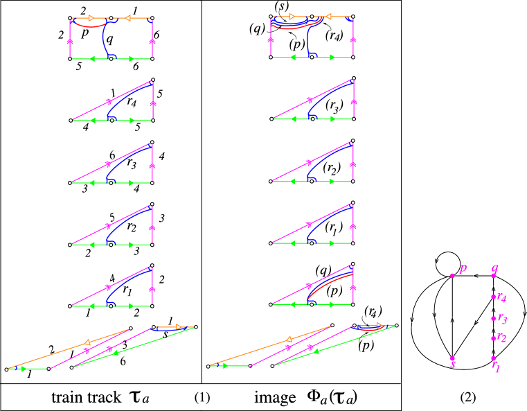
Figure 26. (1) $\tau_{a}\subset F_{a}$ and $\Phi_{a}(\tau_{a})$ (up to isotopy) (2) $\Gamma_{a}$ for $a=(1,4,1)_{+}$.

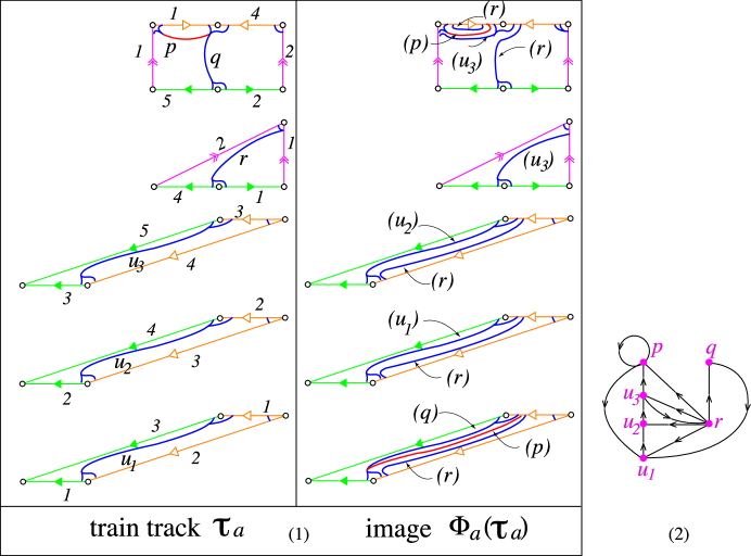
Figure 27. (1) $\tau_{a}\subset F_{a}$ and $\Phi_{a}(\tau_{a})$ (up to isotopy) (2) $\Gamma_{a}$ for $a=(3,1,1)_{-}$.

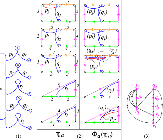
Figure 28. (1) $\tau_{a}$ (2) Another description of $\tau_{a}\subset F_{a}$ and $\Phi_{a}(\tau_{a})$ (up to isotopy) (3) $\Gamma_{a}$ for $a=(2,3)_{0}$.

4.3. Infinite sequences of fibered classes

We exhibit several infinite sequences of fibered classes of $N$, each of which corresponds to a subsequence of pseudo-Anosovs to give the upper bounds (U1), $\cdots$, (U6) except (U3) in Table 1. Each sequence lies on the section either $S_{\beta}(r)$ for $r\in\{\tfrac{3}{-2},-1,\tfrac{1}{-2}\}$ or $S_{\gamma}(r)$ for $r\in\{1,\infty\}$. A sequence of fibered classes in $S_{\beta}(\tfrac{3}{-2})$ (resp. $S_{\gamma}(1)$, $S_{\beta}(\tfrac{1}{-2})$) defines the sequence of fibered classes of the hyperbolic Dehn filling $N(\tfrac{3}{-2})$ (resp. $N(1)$, $N(\tfrac{1}{-2})$). We indicate where each sequence sits on the fibered face $\Delta$, see Figure 29. The purpose of the following examples is to construct the invariant train track $\tau_{a}$, the induced directed graph $\Gamma_{a}$ and curve complex $G_{a}$ associated to each fibered class $a$ in each infinite sequence concretely and to see a structure of the monodromy $\Phi_{a}$ of the fibration associated to $a$ via the curve complex $G_{a}$. We will see that the topological type of $G_{a}$ is fixed and it is either $K_{1,2}^{**}$ or $K_{1,3}^{**}$ for each infinite sequence.

Other sequences of fibered classes of $N$ with small dilatations can be found in [16, Section 5].

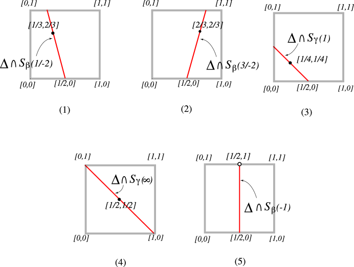
Figure 29. (1) $\Delta\cap S_{\beta}(\tfrac{1}{-2})$. (2) $\Delta\cap S_{\beta}(\tfrac{3}{-2})$. (3) $\Delta\cap S_{\gamma}(1)$. (4) $\Delta\cap S_{\gamma}(\infty)=\Delta_{0}$. (5) $\Delta\cap S_{\beta}(-1)$.

Example 4.2 (Figure 30).

Suppose that $g\equiv 2,4$ $\pmod{6}$. Take a sequence of primitive fibered classes

$$a_{g}=(1,g+2,g-1)_{+}=(g,2g+2,1)\in S_{\beta}(\tfrac{1}{-2}).$$

(The fibered class in Example 4.1(1) is equal to $a_{2}$ in the present example.) Observe that the projections $[a_{g}]$’s go to $[\tfrac{1}{3},\tfrac{2}{3}]\in int(\Delta)$ as $g$ goes to $\infty$, see Figure 29(1). By Lemma 2.6(3)(7), it was shown in [19] that the fiber $F_{a_{g}}$ has genus $g$, and $\mathcal{F}_{a_{g}}$ is orientable. The dilatation $\lambda_{(1,g+2,g-1)_{+}}$ is equal to the largest root of

$$Q_{(1,g+2,g-1)_{+}}(t)=(t^{g+1}+1)(t^{2g}-t^{g+1}-t^{g}-t^{g-1}+1).$$

Since $\mathcal{F}_{a_{g}}$ is orientable, the monodromy $\Phi_{a_{g}}:F_{a_{g}}\rightarrow F_{a_{g}}$ of the fibration associated to $a_{g}$ extends canonically to the pseudo-Anosov homeomorphism $\widehat{\Phi}_{g}$ on the closed surface $\varSigma_{g}$ of genus $g$ with the dilatation $\lambda_{(1,g+2,g-1)_{+}}$. We now introduce the Lanneau-Thiffeault polynomial

$$f_{(a,b)}(t)=t^{2a}-t^{a+b}-t^{a}-t^{a-b}+1.$$

Then $f_{(g,1)}(t)$ is a factor of $Q_{(1,g+2,g-1)_{+}}(t)$. If we set $\lambda_{(g,1)}$ to be the largest root of $f_{(g,1)}(t)$, then we have $\lambda_{(g,1)}=\lambda_{(1,g+2,g-1)_{+}}=\lambda(\widehat{\Phi}_{g})$. It is known that $\delta_{2}^{+}=\lambda_{(2,1)}$ [39], $\delta_{4}^{+}=\lambda_{(4,1)}$ [22] and $\delta_{8}^{+}=\lambda_{(8,1)}$ [22, 10]. Lanneau and Thiffeault asked in [22] whether the equality $\delta_{g}^{+}=\lambda_{(g,1)}$ holds for even $g$. The existence of pseudo-Anosovs $\widehat{\Phi}_{g}$ for $g\equiv 2,4$ $\pmod{6}$ in the present example were discovered by Hironaka in [10], see also Remark 1.3. The sequence of pseudo-Anosovs $\{\widehat{\Phi}_{g}\}$ can be used for a subsequence to prove both upper bounds (U1) and (U2) in Table 1. In fact we have

$$\lim_{g\to\infty}g\log\lambda(\widehat{\Phi}_{g})=\log(\tfrac{3+\sqrt{5}}{2}).$$

Example 4.3 (Figure 31).

An explicit value of $\delta_{7}^{+}$ is known. The lower bound of $\delta_{7}^{+}$ was given in [22] and an example which realizes this lower bound was found in [1] and [19] independently. However an explicit construction of a minimizer of $\delta_{7}^{+}$ was not given in [1, 19]. Here we construct such a minimizer. Suppose that $g\equiv 7,9\pmod{10}$. Following [19], we take a sequence of primitive fibered classes

$$a_{g}=(g+6,2,g)_{+}=(2g+6,2g+8,g+6)\in S_{\beta}(\tfrac{3}{-2}).$$

Then $F_{a_{g}}$ has genus $g$ ([19]) and the projections $[a_{g}]$’s go to $[\tfrac{2}{3},\tfrac{2}{3}]\in int(\Delta)$ as $g$ goes to $\infty$, see Figure 29(2). We have

$$Q_{(g+6,2,g)_{+}}(t)=(t^{g+4}+1)(t^{2g+4}-t^{g+4}-t^{g+2}-t^{g}+1),$$

and the dilatation $\lambda_{(g+6,2,g)_{+}}$ is equal to the largest root of this polynomial. In particular $\lambda_{(g+6,2,g)_{+}}$ is equal to the largest root of the second factor of $Q_{(g+6,2,g)_{+}}(t)$. Lemma 2.6(7) ensures that the monodromy $\Phi_{a_{g}}:F_{a_{g}}\rightarrow F_{a_{g}}$ of the fibration associated to $a_{g}$ extends to the pseudo-Anosov $\widehat{\Phi}_{g}:\varSigma_{g}\rightarrow\varSigma_{g}$ with orientable invariant foliations. It is known that $\delta_{7}^{+}$ is equal to the largest root of the second factor of $Q_{(13,2,7)_{+}}(t)$ as above. Hence $\delta_{7}^{+}=\lambda_{(13,2,7)_{+}}$, and the extension $\widehat{\Phi}_{7}$ of ${\Phi}_{(13,2,7)_{+}}$ is a minimizer of $\delta_{7}^{+}$. The existence of the sequence of pseudo-Anosovs $\{\widehat{\Phi}_{g}\}$ was discovered in [1, 19]. We have

$$\lim_{g\to\infty}g\log\lambda(\widehat{\Phi}_{g})=\log(\tfrac{3+\sqrt{5}}{2}),$$

see the upper bounds (U1) and (U2).

Example 4.4 (Figure 32).

Suppose that $g\equiv 1,5\pmod{10}$. Following [19], we take a sequence of primitive fibered classes

$$a_{g}=(g+10,4,g-2)_{+}=(2g+8,2g+12,g+10)\in S_{\beta}(\tfrac{3}{-2}).$$

Then the fiber $F_{g}$ has genus $g$ ([19]), and the dilatation $\lambda_{(g+10,4,g-2)_{+}}$ is equal to the largest root of

$$Q_{(g+10,4,g-2)_{+}}(t)=(t^{g+6}+1)(t^{2g+4}-t^{g+6}-t^{g+2}-t^{g-2}+1).$$

Observe that the projections $[a_{g}]$’s go to $[\tfrac{2}{3},\tfrac{2}{3}]\in int(\Delta)$ as $g$ goes to $\infty$, see Figure 29(2). We see that the monodromy $\Phi_{a_{g}}:F_{a_{g}}\rightarrow F_{a_{g}}$ of the fibration associated to $a_{g}$ extends to the pseudo-Anosov $\widehat{\Phi}_{g}$ on $\varSigma_{g}$ with orientable invariant foliations. The dilatation of $\widehat{\Phi}_{g}$ is same as the dilatation of $\Phi_{a_{g}}$, that is $\lambda_{(g+10,4,g-2)_{+}}$. The equality $\delta_{5}^{+}=\lambda_{(15,4,3)_{+}}$ holds, see [22]. The sequence of pseudo-Anosovs $\{\widehat{\Phi}_{g}\}$ satisfies

$$\lim_{g\to\infty}g\log\lambda(\widehat{\Phi}_{g})=\log(\tfrac{3+\sqrt{5}}{2}),$$

see the upper bounds (U1) and (U2).

Example 4.5 (Figure 33).

Following [17], we take a sequence of primitive fibered classes

$$a_{n}=(2n-1,1,n-1)_{-}=(n-1,n,-2n+1)\in S_{\gamma}(1).$$

The dilatation $\lambda_{(2n-1,1,n-1)_{-}}$ is equal to the largest root of

$$Q_{(2n-1,1,n-1)_{-}}(t)=t^{4n-2}-t^{3n-1}-t^{3n-2}-t^{n}-t^{n-1}+1.$$

The projections of $a_{n}$’s go to $[\tfrac{1}{4},\tfrac{1}{4}]\in int(\Delta)$ as $n$ goes to $\infty$, see Figure 29(3). We find that $a_{n}$ defines a fibered class $\overline{a_{n}}\in H_{2}(N_{\gamma}(1),\partial N_{\gamma}(1))$, see the beginning of Section 4. By using Lemma 2.6(6), we see that the monodromy of the fibration on $N(1)$ associated to $\overline{a_{n}}$ has the dilatation $\lambda_{(2n-1,1,n-1)_{-}}$. Observe that the topological type of the fiber (i.e, minimal representative) of $\overline{a_{n}}$ is homeomorphic to $\varSigma_{1,2n-1}$. The sequence of the monodromies $\Phi_{\overline{a_{n}}}$ of fibrations associated to $\overline{a_{n}}$’s on the Whitehead link exterior $N_{\gamma}(1)$ can be used for a subsequence to prove (U5). In fact, we have

$$\lim_{n\to\infty}(2n-1)\log\lambda(\Phi_{\overline{a_{n}}})=2\log\delta(D_{4}).$$

Example 4.6 (Figure 34).

For $n\geq 3$, consider a sequence of primitive fibered classes

$$a_{n}=(1,n-1)_{0}=(n-1,n,0)\in S_{\gamma}(\infty),$$

which is studied in [18]. We see that $F_{a_{n}}$ is homeomorphic to $\varSigma_{0,2n+1}$. The projection of $a_{n}$ goes to $[\tfrac{1}{2},\tfrac{1}{2}]\in int(\Delta)$ as $n$ goes to $\infty$, see Figure 29(4). The dilatation $\lambda_{(1,n-1)_{0}}$ equals the largest root of

$$Q_{(1,n-1)_{0}}(t)=t^{2n-1}-2(t^{n-1}+t^{n})+1.$$

By using the same arguments as in Example 4.1(3), we see that the monodromy $\Phi_{a_{n}}:\varSigma_{0,2n+1}\rightarrow\varSigma_{0,2n+1}$ of the fibration associated to $a_{n}$ defines the pseudo-Anosov $\overline{\Phi}_{a_{n}}:D_{2n-1}\rightarrow D_{2n-1}$ with the same dilatation $\lambda_{(1,n-1)_{0}}$. Such a pseudo-Anosov homeomorphism $\overline{\Phi}_{a_{n}}:D_{2n-1}\rightarrow D_{2n-1}$ is studied in [14]. It is known that $\delta(D_{5})=\lambda_{(1,2)_{0}}$, see [9] and $\delta(D_{7})=\lambda_{(1,3)_{0}}$, see [23]. The sequence of pseudo-Anosovs $\{\Phi_{a_{n}}:\varSigma_{0,2n-1}\rightarrow\varSigma_{0,2n-1}\}$ can be used for a subsequence to prove (U4):

$$\lim_{n\to\infty}(2n-1)\log\lambda(\Phi_{a_{n}})=2\log(2+\sqrt{3}).$$

Example 4.7 (Figure 35).

For $n\geq 2$, let us consider a sequence of fibered classes

$$a_{n}=(2,2n-1)_{0}=(2n-1,2n+1,0)\in S_{\gamma}(\infty),$$

which is studied in [18]. (The fibered class in Example 4.1(3) is equal to $a_{2}$ in the present example.) We see that $F_{a_{n}}$ is homeomorphic to $\varSigma_{0,4n+2}$. The projection of $a_{n}$ goes to $[\tfrac{1}{2},\tfrac{1}{2}]\in int(\Delta)$ as $n$ goes to $\infty$. The dilatation $\lambda_{(2,2n-1)_{0}}$ equals the largest root of

$$Q_{(2,2n-1)_{0}}(t)=t^{4n}-2(t^{2n-1}+t^{2n+1})+1.$$

By using the same arguments as in Example 4.1(3), we see that the monodromy $\Phi_{a_{n}}:\varSigma_{0,4n+2}\rightarrow\varSigma_{0,4n+2}$ of the fibration associated to $a_{n}$ defines the pseudo-Anosov $\overline{\Phi}_{a_{n}}:D_{4n}\rightarrow D_{4n}$ with the dilatation $\lambda_{(2,2n-1)_{0}}$. As we have seen in Example 4.1(3) that $\delta(D_{8})=\lambda_{(2,3)_{0}}$ holds. Such a pseudo-Anosov homeomorphism $\overline{\Phi}_{a_{n}}:D_{4n}\rightarrow D_{4n}$ is also studied in [38]. The sequence of pseudo-Anosovs $\{\Phi_{a_{n}}:\varSigma_{0,4n+2}\rightarrow\varSigma_{0,4n+2}\}$ can be used for a subsequence to prove (U4):

$$\lim_{n\to\infty}(4n+2)\log\lambda(\Phi_{a_{n}})=2\log(2+\sqrt{3}).$$

Example 4.8 (Figure 36).

Throughout this example, we fix $g\geq 0$. The following sequence of fibered classes is used for the proof of Theorem 1.1, see [20]:

$$a_{(g,p)}=(p-g,p-g,2g+1)_{+}=(p+g+1,2p+1,p-g)\in S_{\beta}(-1).$$

The projections $[a_{(g,p)}]$’s go to $[\tfrac{1}{2},1]\in\partial\Delta$ as $p$ goes to $\infty$, see Figure 29(5). It is not hard to see that $a_{(g,p)}$ is primitive if and only if $2g+1$ and $p+g+1$ are relatively prime. If $a_{(g,p)}$ is primitive, then the fiber $F_{a_{(g,p)}}$ is homeomorphic to $\varSigma_{g,2p+4}$, and we have

$$\sharp(\partial_{\beta}F_{(g,p)})=2p+1\ \mbox{and}\ \sharp(\partial_{\alpha}F_{(g,p)})+\sharp(\partial_{\gamma}F_{(g,p)})=3.$$

There exists a sequence of primitive fibered classes $\{a_{(g,p_{i})}\}_{i=0}^{\infty}$ with $p_{i}\to\infty$ when $i\to\infty$, where $p_{i}$ depends on $g$. (For example, take $p_{i}=(g+1)+i(2g+1)$.) This means that $F_{a_{(g,p_{i})}}$ has genus $g$ and the number of the boundary components of $F_{a_{(g,p_{i})}}$ (which is equal to $2p_{i}+4$) goes to $\infty$ as $i$ does. As we have seen above, the projection of such a class $a_{(g,p_{i})}$ goes to the same point $[\tfrac{1}{2},1]\in\partial\Delta$ (which does not depend on $g$) as $p_{i}$ goes to $\infty$.

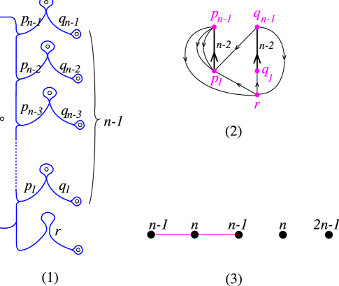
Figure 34. Example 4.6. (1) $\tau_{a_{n}}$ (circles indicate components of $\partial F_{a_{n}}$) (2) $\Gamma_{a_{n}}$ (3) $G_{a_{n}}$ for $a_{n}=(1,n-1)_{0}$.

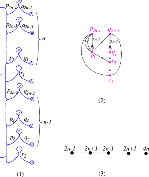
Figure 35. Example 4.7. (1) $\tau_{a_{n}}$ (2) $\Gamma_{a_{n}}$ (3) $G_{a_{n}}$ for $a_{n}=(2,2n-1)_{0}$.

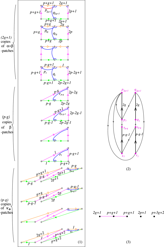
Figure 36. Example 4.8. (1) $\tau_{a_{(g,p)}}\subset F_{a_{(g,p)}}$ (2) $\Gamma_{a_{(g,p)}}$ (3) $G_{a_{(g,p)}}$ for $a_{(g,p)}=(p-g,p-g,2g+1)_{+}$.

References

- [1] J. W. Aaber and N. M. Dunfield, Closed surface bundles of least volume, Algebraic and Geometric Topology 10 (2010), 2315-2342.
- [2] M Bestvina, M Handel, Train–tracks for surface homeomorphisms, Topology 34 (1994) 1909-140.
- [3] J. Birman, PA mapping classes with minimum dilatation and Lanneau-Thiffeault polynomials, preprint.
- [4] J. H. Cho and J. Y. Ham, The minimal dilatation of a genus-two surface, Experimental Mathematics 17 (2008), 257-267.
- [5] A. Fathi, F. Laudenbach and V. Poenaru, Travaux de Thurston sur les surfaces, Astérisque, 66-67, Société Mathématique de France, Paris (1979).
- [6] D. Fried, Fibrations over with pseudo-Anosov monodromy, Exposé 14 in ‘Travaux de Thurston sur les surfaces’ by A. Fathi, F. Laudenbach and V. Poenaru, Astérisque, 66-67, Société Mathématique de France, Paris (1979), 251-266.
- [7] D. Fried, Flow equivalence, hyperbolic systems and a new zeta function for flows, Commentarii Mathematici Helvetici 57 (1982), 237-259.
- [8] F. R. Gantmacher, Matrix Theory, Vol. 2, American Mathematical Society (2000).
- [9] J. Y. Ham and W. T. Song, The minimum dilatation of pseudo-Anosov -braids, Experimental Mathematics 16 (2007), 167-179.
- [10] E. Hironaka, Small dilatation mapping classes coming from the simplest hyperbolic braid, Algebraic and Geometric Topology 10 (2010), 2041-2060.
- [11] E. Hironaka, Mapping classes associated to mixed-sign Coxeter graphs, preprint.
- [12] E. Hironaka, Quotient families of mapping classes, preprint.
- [13] E. Hironaka, Small dilatation pseudo-Anosov mapping classes and short circuits on train track automata, Mittag-Leffler Institute Preprint Collection, Workshop on Growth and Mahler Measures in Geometry and Topology (2013), 17-41.
- [14] E. Hironaka and E. Kin, A family of pseudo-Anosov braids with small dilatation, Algebraic and Geometric Topology 6 (2006), 699-738.
- [15] N. V. Ivanov, Stretching factors of pseudo-Anosov homeomorphisms, Journal of Soviet Mathematics, 52 (1990), 2819–2822, which is translated from Zap. Nauchu. Sem. Leningrad. Otdel. Mat. Inst. Steklov. (LOMI), 167 (1988), 111-116.
-
[16]
E. Kin,
Notes on pseudo-Anosovs with small dilatations coming from the magic 3-manifold,
Representation spaces, twisted topological invariants and geometric structures of 3-manifolds,
RIMS Kokyuroku 1836 (2013), 45-64.
available at
http://www.kurims.kyoto-u.ac.jp/~kyodo/kokyuroku/contents/pdf/1836-05.pdf - [17] E. Kin, S. Kojima and M. Takasawa, Minimal dilatations of pseudo-Anosovs generated by the magic -manifold and their asymptotic behavior, Algebraic and Geometric Topology 13 (2013), 3537-3602.
- [18] E. Kin and M. Takasawa, Pseudo-Anosov braids with small entropy and the magic -manifold, Communications in Analysis and Geometry 19 Number 4 (2011), 1-54.
- [19] E. Kin and M. Takasawa, Pseudo-Anosovs on closed surfaces having small entropy and the Whitehead sister link exterior, Journal of the Mathematical Society of Japan 65, Number 2 (2013), 411-446.
- [20] E. Kin and M. Takasawa, The boundary of a fibered face of the magic -manifold and the asymptotic behavior of the minimal pseudo-Anosovs dilatations. arXiv:1205.2956
- [21] K. H. Ko, J. Los and W. T. Song, Entropies of braids, Journal of Knot Theory and its Ramifications 11 (2002), 647-666.
- [22] E. Lanneau and J. L. Thiffeault, On the minimum dilatation of pseudo-Anosov homeomorphisms on surfaces of small genus, Annales de l’Institut Fourier 61 (2011), 105-144.
- [23] E. Lanneau and J. L. Thiffeault, On the minimum dilatation of braids on the punctured disc, Geometriae Dedicata 152 (2011), 165-182.
- [24] D. Long and U. Oertel, Hyperbolic surface bundles over the circle, Progress in knot theory and related topics, Travaux en Course 56, Hermann, Paris (1997), 121-142.
- [25] J. Los, Infinite sequence of fixed-point free pseudo-Anosov homeomorphisms, Ergodic Theory and Dynamical Systems 30 (2010), 1739-1755.
- [26] B. Martelli and C. Petronio, Dehn filling of the “magic” -manifold, Communications in Analysis and Geometry 14 (2006), 969-1026.
- [27] S. Matsumoto, Topological entropy and Thurston’s norm of atoroidal surface bundles over the circle, Journal of the Faculty of Science, University of Tokyo, Section IA. Mathematics 34 (1987), 763-778.
- [28] C. McMullen, Polynomial invariants for fibered -manifolds and Teichmüler geodesic for foliations, Annales Scientifiques de l’École Normale Supérieure. Quatrième Série 33 (2000), 519-560.
- [29] C. McMullen, Entropy and the clique polynomial, preprint.
- [30] H. Minakawa, Examples of pseudo-Anosov homeomorphisms with small dilatations, The University of Tokyo. Journal of Mathematical Sciences 13 (2006), 95-111.
- [31] U. Oertel, Homology branched surfaces: Thurston’s norm on , LMS Lecture Note Series 112, Low-dimensional Topology and Kleinian Groups, Editor D. B. A. Epstein (1986), 253-272.
- [32] U. Oertel, Affine laminations and their stretch factores, Pacific Journal of Mathematics 182 (2) (1997), 303-328.
- [33] A. Papadopoulos and R. Penner, A characterization of pseudo-Anosov foliations, Pacific Journal of Mathematics 130 (2) (1987), 359-377.
- [34] R. C. Penner, Bounds on least dilatations, Proceedings of the American Mathematical Society 113 (1991), 443-450.
- [35] W. Thurston, A norm of the homology of -manifolds, Memoirs of the American Mathematical Society 339 (1986), 99-130.
- [36] W. Thurston, Hyperbolic structures on 3-manifolds II: Surface groups and 3-manifolds which fiber over the circle, preprint, arXiv:math/9801045
- [37] C. Y. Tsai, The asymptotic behavior of least pseudo-Anosov dilatations, Geometry and Topology 13 (2009), 2253-2278.
- [38] R. Venzke, Braid forcing, hyperbolic geometry, and pseudo-Anosov sequences of low entropy, PhD thesis, California Institute of Technology (2008).
- [39] A. Y. Zhirov, On the minimum dilation of pseudo-Anosov diffeomorphisms on a double torus, Russian Mathematical Surveys 50 (1995), 223-224.