Real time dynamics and proposal for feasible experiments of lattice gauge-Higgs model simulated by cold atoms

Abstract

Lattice gauge theory has provided a crucial non-perturbative method in studying canonical models in high-energy physics such as quantum chromodynamics. Among other models of lattice gauge theory, the lattice gauge-Higgs model is a quite important one because it describes wide variety of phenomena/models related to the Anderson-Higgs mechanism such as superconductivity, the standard model of particle physics, and inflation process of the early universe. In this paper, we first show that atomic description of the lattice gauge model allows us to explore real time dynamics of the gauge variables by using the Gross-Pitaevskii equations. Numerical simulations of the time development of an electric flux reveal some interesting characteristics of dynamical aspect of the model and determine its phase diagram. Next, to realize a quantum simulator of the U(1) lattice gauge-Higgs model on an optical lattice filled by cold atoms, we propose two feasible methods: (i) Wannier states in the excited bands and (ii) dipolar atoms in a multilayer optical lattice. We pay attentions to respect the constraint of Gauss’s law and avoid nonlocal gauge interactions.

I Introduction

Cold atoms in an optical lattice have been used as versatile quantum simulators for various many-body quantum systems and some important results were obtained book . Recently, there appeared several proposals to simulate models of lattice gauge theory (LGT) KK-wilson ; KK-kogut ; Wiese . Since its introduction, LGT has been an indispensable tool to studying the non-perturbative aspect of quantum models in the high-energy physics (HEP) such as confinement of quarks, the spontaneous chiral-symmetry breaking, etc. Atomic simulations, if realized, shall certainly clarify the dynamics, i.e, the time evolution of lattice gauge models, which is far beyond the present theoretical standard.

At present, the proposals are classified into two approaches. In the first approach Zohar2 ; Tagliacozzo1 ; Banerjee1 ; Zohar3 ; Zohar4 ; Banerjee2 ; Tagliacozzo2 , atoms with spin degrees of freedom are put on links of the optical lattice. Such a lattice gauge model is called the “quantum link model” or “gauge magnet” Horn ; Orland ; Chandrasekharan . Although the Gauss’s law (divergence of the electric field is just the charge density of matter fields) KK-ks is assured as the conservation of “angular momentum” Zohar5 , the Hilbert space of this model itself truncates the full Hilbert space of the original U(1) LGT studied in HEP.

In the second approach Zohar1 , one considers the Bose-Einstein condensate (BEC) of atoms put on each link of the two or three dimensional optical lattice. The U(1) phase variable of the complex amplitude of BEC plays a role of dynamical gauge field on the links, and its density fluctuation corresponds to the electric field, the conjugate variable of the gauge field Zohar1 ; KK-Tewari . Adopting the phase variable of the atomic field as the gauge field assures us that we deal with a U(1) field as in HEP in contrast with the first approach. However, to keep the Gauss’s law and the short-range gauge interactions simultaneously, a complex design of the system and also a fine tuning of interaction parameters are generally needed in the experimental setups Zohar1 ; KK-Tewari .

Recently, we proposed a perspective to overcome the difficulty to respect the local gauge invariance in the second approach Kasamatsu . Namely, the cold atomic simulator of the LGT without exact local gauge invariance due to untuned interaction parameters (the Gauss’s law is not satisfied) can be a simulator for a lattice “gauge-Higgs” (GH) model KK-complementarity with exact local gauge invariance, where the unwelcome interactions that violate the Gauss’s law are viewed as gauge-invariant couplings of the gauge field to a Higgs field.

Needless to say, the GH model is a canonical model of Anderson-Higgs mechanism and plays a very important role in various fields of modern physics. Its list includes mass generation in the standard model of HEP, phase transition and the vortex dynamics btj in superconductivity, time-evolution of the early universe such as the dynamics of Higgs phase transition and the related problems of topological defects, uniformity, etc. inflation1 ; inflation2 . Atomic quantum simulation of this model is certainly welcome because it simulates the real time evolution of the above exciting phenomena.

In what follows, we consider the second approach to discuss the atomic quantum simulator of the U(1) lattice GH model by using cold atoms in a two-dimensional (2D) optical lattice. Our target GH model has a nontrivial phase structure, i.e., existence of the phase boundary between confinement and Higgs phases, and this phase boundary is to be observed by cold-atom experiments. In the experiments, each phase could be generally studied through the non-equilibrium dynamics of the system, which are detected by e.g., the density distribution of the time-of-flight imaging after the system is perturbed. As a reference to such experiments, we make numerical simulations of the time-dependent Gross-Pitaevskii (GP) equation and observe the real-time dynamics of the atomic simulators. In particular, we study the dynamical stability of a single electric flux connecting two charges with opposite signs, corresponding to a density hump and dip for the atomic simulators. We stress that this dynamical simulation in an interacting atomic system gives a new theoretical tool for the analysis of lattice gauge models far beyond the present standards of the theoretical study on the LGT using the “classical” Monte-Carlo simulations, the strong-coupling expansion, etc. The obtained phase boundary is discussed and compared with that of the Monte-Carlo simulations. Next, we propose two realistic experimental setup for the quantum simulators. To respect the constraint of Gauss’s law and avoid nonlocal gauge interactions, it is necessary to tune suitably the intersite density-density interaction of the hamiltonian. We give two ideas: (i) Using Wannier states in the excited bands and (ii) Using dipolar atoms in a multilayer optical lattice, both of which are reachable under current experimental techniques.

The paper is organized as follows. In Sec.II, we introduce our target hamiltonian of the U(1) lattice GH model starting from the extended Bose-Hubbard (BH) model with the intersite density-density interaction. The exact correspondence of the atomic system to the LGT has been discussed in Ref. Kasamatsu . In Sec. III, we present the results of the dynamical simulations by means of the GP equation, which is obtained under the saddle-point approximation of the real-time path integral of the two quantum hamiltonians, i.e., the original BH model and the target GH model. The obtained dynamical phase diagram is compared with the result of the Monte-Carlo simulations. We give two proposals for experiments to construct realistic atomic simulators for the lattice GH model in Sec. IV. Method A in Sec. IV.1 relies on extended orbits of the Wannier functions in excited bands of an optical lattice. Another method B utilize the long-range interaction between atoms in different layers of 2D optical lattices. Both methods may be possible to tune the intersite density-density interactions in the 2D BH system for our purpose. Section V is devoted to our conclusion and an outlook on future direction.

II From Bose-Hubbard model to the gauge-Higgs model

Corresponding to the simplest realistic experimental situation of the quantum simulator, we focus on the boson system defined on a 2D square lattice. We start from a generalized BH hamiltonian book

$$\hat{H}=-\sum_{k,a\neq b}J_{ab}\hat{\psi}_{a}^{{\dagger}}\hat{\psi}_{b}+\frac{V_{0}}{4}\sum_{k,a}\hat{\rho}_{a}(\hat{\rho}_{a}-1)+\sum_{k,a\neq b}\frac{V_{ab}}{2}\hat{\rho}_{a}\hat{\rho}_{b},$$ (1)

which describes the bosons in a single band of a 2D optical lattice. The bosonic atomic fields $\hat{\psi}_{a}=\exp(i\hat{\theta}_{a})\sqrt{\hat{\rho}_{a}}$ are put on the site $a$ of the square optical lattice. The summation is taken over the unit cell $k$ (yellow region in Fig. 1) and, in each unit cell, over the the site $a(b)\in 1$-6. We confine ourselves to the nearest-neighbor (NN) and next-nearest-neighbor (NNN) couplings for the site pairs $(a,b)$ in the 1st and 3rd terms. The parameters $J_{ab}(=J_{ba})$, $V_{0}$, and $V_{ab}(=V_{ba})$ are the coefficients of the hopping, the on-site interaction, and the intersite interaction, respectively, and calculable by using the Wannier functions in a certain band. The intersite terms $V_{ab}$ may arise when the atoms have a long-range dipole-dipole interaction (DDI) dipolerev , or when the atoms are populated in the excited bands of the optical lattice Scarola .

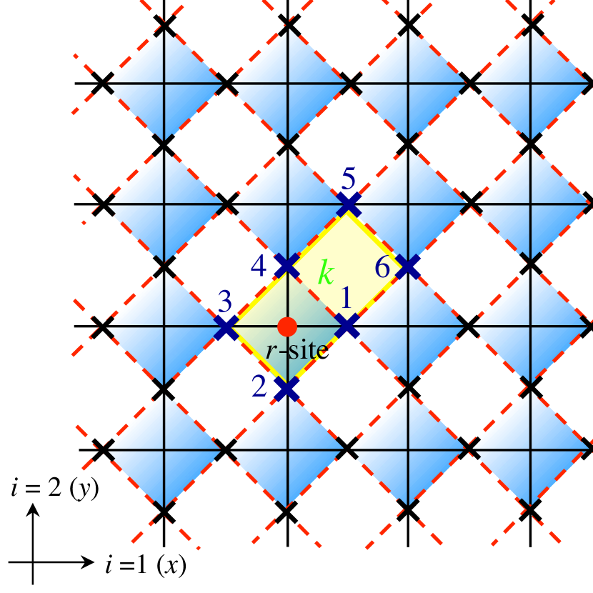
Figure 1: Relation between two 2D lattices. The dashed red lines indicate the 2D optical lattice with the square geometry, and cold atoms reside on its sites denoted by black crosses. Its unit cell consists of a pair of white and blue squares (yellow region). The filled black lines indicate the 2D gauge lattice on which the U(1) lattice GH model is defined. Then the cold atoms are viewed to sit on each link of the gauge lattice to play the role of gauge field. The relevant sites of the original lattice (links among the site $r$ of the gauge lattice) in Table 1 are numbered as $a=1\sim 6$, as $a=1=(r,1)$, $2=(r-2,2)$, $3=(r-1,1)$, $4=(r,2)$, $5=(r+2,1)$, $6=(r+1,2)$, where $(r,i)$ represents the link of the gauge lattice emanating from the site $r$ into the positive $i\ (=1,2)$-th direction. The gauge lattice plays an important role also in the study of the BH model with $V_{ab}=0$ in a different context mielke .

Table 1: Atomic parameters $J_{ab}$ and $V_{ab}$ in Eq. (1). Those not shown below are set to zero to avoid double counting [$(1,6)$, etc.] or due to longer-ranges [$(3,5)$, etc].

group	range	$(a,b)$	$J_{ab}$	$V_{ab}$
(i)	NN	(1,2), (2,3), (3,4), (1,4)	$J$	$\gamma^{-2}$
(ii)	1st half of NNN	(1,3), (2,4)	$J^{\prime}$	$\gamma^{-2}$
(iii)	2nd half of NNN	(1,5), (4,6)	$J^{\prime\prime}$	0

To map the BH model onto the hamiltonian of LGT, we consider the diagonal lattice whose sites $r=(r_{1},r_{2})$ are positioned on the centers of the colored squares in Fig. 1. Then, the original sites can be viewed as links of the diagonal lattice. The links are labeled as $(r,i)$ with the direction index $i=1,2$. To derive the hamiltonian of the target GH model, we consider the case such that $J_{ab}$ and $V_{ab}$ take values according to the following three groups (i)-(iii) for pairs $(a,b)$ of sites as shown in Table 1 Zohar1 ; Kasamatsu . We note that Table 1 breaks the translational symmetry of atomic interactions, e.g., $V_{24}\neq 0$ while $V_{15}=0$. Next, we assume that the equilibrium atomic density is uniform and sufficiently large $\rho_{0}\equiv\langle\hat{\rho}_{r,a}\rangle\gg 1$. Then, we expand the density operator as $\hat{\rho}_{r,i}=\rho_{0}+\hat{\eta}_{r,i}$, and keep terms up to $O(\hat{\eta}^{2})$ to obtain

$$\hat{H} \simeq\frac{1}{2\gamma^{2}}\sum_{r}\left[\sum_{i}(\hat{\eta}_{r,i}+\hat{\eta}_{r-i,i})\right]^{2}+\frac{V_{0}^{\prime}}{2}\sum_{r,i}\hat{\eta}_{r,i}^{2}$$

$$-\rho_{0}J\sum_{r,i,\delta}\cos(\hat{\theta}_{r,i}-\hat{\theta}_{r,\delta})-2\rho_{0}J^{\prime}\sum_{r,i}\cos(\hat{\theta}_{r,i}-\hat{\theta}_{r-i,i})$$

$$-2\rho_{0}J^{\prime\prime}\sum_{r,i}\cos(\hat{\theta}_{r,i}-\hat{\theta}_{r-\bar{i},i}),$$ (2)

where $V^{\prime}_{0}\equiv V_{0}-2\gamma^{-2}>0$, $(r,\delta)$ represents the NN links of $(r,i)$, and $\bar{1}\equiv 2$, $\bar{2}\equiv 1$. The first order term $O(\hat{\eta})$ is absent due to the stability condition for $\rho_{0}=[\mu+4J+2(J^{\prime}+J^{\prime\prime})]/(V_{0}^{\prime}+8\gamma^{-2})$ with the chemical potential $\mu$. In the atomic simulators of LGT, the phase $\hat{\theta}_{r,i}$ plays a role of a gauge variable on the link $(r,i)$ and its conjugate momentum $\hat{\eta}_{r,i}$ is the electric field $-\hat{E}_{r,i}$ Zohar1 ; KK-Tewari ; Kasamatsu . By replacing $\hat{\eta}_{r,i}\to(-)^{r}\hat{\eta}_{r,i}$ and $\hat{\theta}_{r,i}\to(-)^{r}\hat{\theta}_{r,i}$ with $(-)^{r}\equiv(-)^{r_{1}+r_{2}}$, the first term in the rhs of Eq. (2) describes the “Gauss’s law” as $(2\gamma^{2})^{-1}\sum_{r}[\sum_{i}(\hat{\eta}_{r,i}-\hat{\eta}_{r-i,i})]^{2}\simeq(2\gamma^{2})^{-1}\sum_{r}(\nabla\cdot\mathbf{E})^{2}$. The two conditions $V_{\rm(i)}=V_{\rm(ii)}(=\gamma^{-2})$ and $V_{\rm(iii)}=0$ in Table 1 are necessary to generate the $(\nabla\cdot\mathbf{E})^{2}$ term without nonlocal interaction among $E_{r,i}$. If these conditions are not fulfilled, a product $\hat{E}_{r,i}\hat{E}_{r^{\prime},i^{\prime}}$ over the different links appears additionally, and it gives rise to long-range interactions among the gauge field $\theta_{r,i}$ in the target GH model. Although such a model still respects gauge symmetry, we reject it here because all LGTs relevant to HEP are generally models with local-interaction.

In Ref. Kasamatsu , it was shown that the partition function $Z={\rm Tr}\exp(-\beta\hat{H})$ of the atomic model of Eq. (2) is equivalent to that of the GH model. The GH model is the U(1) lattice gauge model on the (2+1)D lattice, and its partition function is given by

$$Z_{\textrm{GH}} =\int[dU][d\phi]\exp(A_{\rm I}+A_{\rm P}+A_{\rm L}+A_{\rm 2I}+A_{\rm I^{2}}),$$

$$A_{\rm I} =\frac{1}{2}\sum_{x,\mu}c_{1\mu}(\bar{\phi}_{x+\mu}U_{x,\mu}\phi_{x}+\mathrm{c.c.}),$$

$$A_{\rm P} =\frac{1}{2}\sum_{x,\mu<\nu}c_{2\mu\nu}(\bar{U}_{x,\nu}\bar{U}_{x+\nu,\mu}U_{x+\mu,\nu}U_{x,\mu}+\mathrm{c.c.}),$$

$$A_{\rm L} =\frac{c_{3}}{2}\sum_{x}\Big{[}\bar{\phi}_{x+1+2}U_{x+1,2}U_{x,1}\phi_{x}$$

$$+\bar{\phi}_{x+2}\bar{U}_{x+2,1}U_{x+1,2}\phi_{x+1}+\bar{\phi}_{x}\bar{U}_{x,2}\bar{U}_{x+2,1}\phi_{x+1+2}$$

$$+\bar{\phi}_{x+1}U_{x,1}\bar{U}_{x,2}\phi_{x+2}+{\rm c.c.}\Big{]},$$

$$A_{\rm 2I} =\frac{c_{4}}{2}\sum_{x}\sum_{i=1,2}\Big{[}\bar{\phi}_{x+i}U_{x,i}U_{x-i,i}\phi_{x-i}+\mathrm{c.c.}\Big{]},$$

$$A_{\rm I^{2}} =\frac{c_{5}}{2}\sum_{x}\Big{[}\bar{\phi}_{x+2+1}U_{x+2,1}\phi_{x+2}\cdot\bar{\phi}_{x+1}U_{x,1}\phi_{x}$$

$$+(1\leftrightarrow 2)+\mathrm{c.c.}\Big{]}.$$ (3)

Here, $x=(x_{0},r_{1},r_{2})$ is the site index of the (2+1)D lattice with the discrete imaginary time $\tau=x_{0}\times\Delta\tau\ [x_{0}=0,\cdots,N_{0},N_{0}\Delta\tau=\beta\equiv(k_{\rm B}T)^{-1}]$ and the 2D spatial coordinate $r_{1},r_{2}$. $\mu$ and $\nu$ $(=0,1,2)$ are direction indices. The U(1) gauge variables $U_{x,\mu}\equiv\exp(i\theta_{x,\mu})$ are defined on the link $(x,\mu)$. $\theta_{x,\mu}\ (\mu=1,2)$ corresponds to the eigenvalue of the phase of atomic operator $\hat{\psi}_{r,a}$ through $\theta_{x,\mu}=\hat{\theta}_{r,i}$. The complex field $\phi_{x}$ defined on site $x$ is a bosonic matter field, referred to “Higgs field” in the London limit, taking the form $\phi_{x}=\exp(i\varphi_{x})$ with frozen radial fluctuations. The integration $\int[dU][d\phi]$ is over the angles $\theta_{x,\mu},\varphi_{x}\in[0,2\pi)$. The coefficients $c_{1}\sim c_{5}$ are real dimensionless parameters for interactions among gauge fields. Each term of the action, hence the action itself, and the integration measure are invariant under the local U(1) gauge transformation, $\theta_{x,\mu}\to\theta_{x,\mu}+\lambda_{x+\mu}-\lambda_{x},\ \varphi_{x}\to\varphi_{x}+\lambda_{x}$.

According to Ref. Kasamatsu , the atomic simulator of the GH model in a 2D system corresponds to the following case of parameters for $c_{1\mu},c_{2\mu\nu}$:

$$c_{10}=c_{1},\hskip 14.22636ptc_{11}=c_{12}=0,$$

$$c_{201}=c_{202}=c_{2},\hskip 14.22636ptc_{212}=0.$$ (4)

In terms of the atomic system, the $c_{1}$- and $c_{2}$-terms describe the sum of the self coupling and the neighboring correlations of densities of atoms, and the $c_{3}$- and $c_{4,5}$-terms describe the NN and the NNN hopping terms respectively. The relations among the parameters of Eq. (2) and Eq. (3) are

$$c_{1}=\frac{\gamma^{2}}{\Delta\tau},\ \ \ \ c_{2}=\frac{1}{\Delta\tau V_{0}^{\prime}},\ \ \ \ c_{3}=2J\rho_{0}\Delta\tau,$$

$$c_{4}=2J^{\prime}\rho_{0}\Delta\tau,\ \ \ \ c_{5}=2J^{\prime\prime}\rho_{0}\Delta\tau,$$ (5)

In experiments, we expect low $T(\lesssim 10$ nK set by the parameters of $\hat{H}$), and the quantum phase transitions may be explored in a multi-dimensional space parametrized by the dimensionless and $\Delta\tau$-independent combinations such as $c_{1}/c_{2}=\gamma^{2}V_{0}^{\prime},c_{3}c_{2}=2J\rho_{0}/V_{0}^{\prime},$ etc.

III Real-time dynamics of simulators: stability of an electric flux

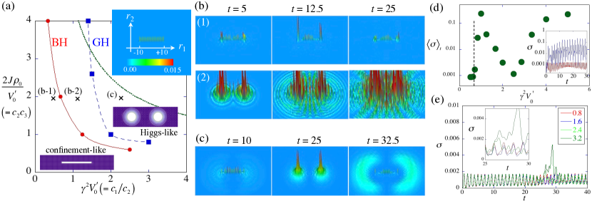
Figure 2: Results of the dynamical simulations. (a) The dynamical phase diagram with respect to the $\Delta\tau$-independent parameters ($\gamma^{2}V_{0}^{\prime}$)-($2J\rho_{0}/V_{0}^{\prime}$) in the BH and GH models. In terms of the GH model Eq. (3), the horizontal and vertical axes correspond to $c_{1}/c_{2}$ and $c_{3}c_{2}$, respectively. The two models give the different phase boundaries, where Higgs (confinement) like behavior can be observed at the right (left) of each boundary. The phase boundary of the BH model is calculated for fixed $\rho_{0}=1$. The dotted curve gives a $\mu=0$ curve for $\rho_{0}=1$, where the amplitude dynamics of the BH model is frozen so that the overall dynamics can coincide to that of the GH model. The upper right inset shows the initial configuration of the squared density $\eta^{2}=(\rho-\rho_{0})^{2}$ in the simulation. We put the density modulation $\eta_{r,1}=(-)^{r}0.1\rho_{0}$ for $-R\leq r_{1}\leq R-1$ with $R=10$. (b) Time development of the density fluctuation $\eta^{2}$ for the BH model. The parameters are given as $(\gamma^{2}V_{0}^{\prime},2J/V_{0}^{\prime})=$ (0.625,2.0) (b-1, upper panels) and $(1.25,2.0)$ (b-2, lower panels), corresponding to the confinement and Higgs regime, respectively (the parameters are also shown in (a) by crosses). The unit of time is chosen as $\hbar/V_{0}^{\prime}$, which is $\sim 0.7$msec for the typical energy scale $V_{0}^{\prime}\sim 10$nK. A flux keeps its initial configuration in the confinement phase (b-1), while it is disappeared by the density fluctuation in the Higgs phase (b-2). (c) The same in (b) for the GH model with the parameter $(\gamma^{2}V_{0}^{\prime},2J\rho_{0}/V_{0}^{\prime})=$ (2.4,2.0) of the Higgs regime. The large amplitude density wave is generated at the point charges, being emitted intermittently. In the confinement phase, the dynamics is similar to Fig. (b-1). (d) Plot of the time average of the remnant of flux $\sigma$ of Eq. (9) for the BH model. The shown results are obtained for $\rho_{0}=1$ and $2J\rho_{0}/V_{0}^{\prime}=2$ and some values of $\gamma^{2}V_{0}^{\prime}$. The vertical dashed line gives the boundary between the confinement (left) and Higgs (right) regime. The inset shows the time evolution of $\sigma(t)$ for (b-1) (red curve) and (b-2) (blue curve). (e) Plot shows the evolution of $\sigma(t)$ for the GH model with $2J\rho_{0}/V_{0}^{\prime}=2$ and several values of $\gamma$ in the legend. The left inset is the enlarged view during $t\in[25,30]$, where $\sigma$ grows intermittently.

In actual experiments observing the nonequilibrium time-evolution of a quantum simulator, the results globally reflect the phase structure of the target model. The (2+1)D GH model supports the confinement phase and the Higgs phase (see Appendix A). The confinement phase is characterized by the strong phase fluctuation; when static two point charges, such as density defects created by the focused potentials, are put on, they are connected by an almost straight electric flux (linearly-rising confinement potential). In contrast, the Higgs phase possesses the phase coherence over the system and the system can be regarded as a superfluid phase; the density wave can propagate around the charges Kasamatsu .

To get some insight on the time-evolution of the system, we study the dynamical features of the simulators through numerical simulations under the mean-field approximation of the two quantum hamiltonians: the base BH model Eq. (1) and the target GH model Eq. (2). The time-dependent equations can be derived from the real-time path-integral formulation under the saddle-point approximation (we put $\hbar=1$). The operators of the original hamiltonian are replaced by the $c$-number fields. We confine ourselves to the models with only NN hopping $J\neq 0$ and $J^{\prime}=J^{\prime\prime}=0$ for simplicity. We note in advance that the mean-field equations necessarily underestimate quantum fluctuations, and their results should be taken as a guide to practical and future experiments which are expected to reveal the real dynamics of quantum systems.

The equation of motion for $\psi$ in the BH model of Eq. (1) can be derived from the Lagrangian $L=-\sum_{r}\sum_{i=1,2}i\psi_{r,i}^{\ast}(d\psi_{r,i}/dt)-H$. It is the discretized version of the GP equation called the discrete nonlinear Schorödinger equation Kevbook and given by

$$i\frac{\partial\psi_{r,i}}{\partial t}=-J(\psi_{r,\bar{i}}+\psi_{r-\bar{i},\bar{i}}+\psi_{r+i,\bar{i}}+\psi_{r+i-\bar{i},\bar{i}})$$

$$+\biggl{[}\left(V_{0}^{\prime}+\frac{2}{\gamma^{2}}\right)|\psi_{r,i}|^{2}+\frac{1}{\gamma^{2}}(|\psi_{r,\bar{i}}|^{2}+|\psi_{r-\bar{i},\bar{i}}|^{2}$$

$$+|\psi_{r+i,\bar{i}}|^{2}+|\psi_{r+i-\bar{i},\bar{i}}|^{2}+|\psi_{r-i,i}|^{2}+|\psi_{r+i,i}|^{2})\biggr{]}\psi_{r,i},$$ (6)

where $i=1,2$ and $\bar{1}\equiv 2,\bar{2}\equiv 1$. The uniform stationary solution can be obtained by substituting $\psi_{r,i}=\psi_{0}e^{-i\mu t}$ as $|\psi_{0}|^{2}=(\mu+4J)/(V_{0}^{\prime}+8\gamma^{-2})$, where $\mu$ is the chemical potential. Since an important quantity to observe the dynamics of electric fluxes is the density fluctuation, we give the equilibrium density $|\psi_{0}|^{2}=\rho_{0}$ by controlling the chemical potential as $\mu=\rho_{0}(V_{0}^{\prime}+8\gamma^{-2})-4J$ and see the evolution of the density fluctuation $\eta=\rho-\rho_{0}$.

The time-dependent equation of motion for $\eta$ and $\theta$ in the GH model of Eq. (2) is derived in the similar way from $L=-\sum_{r,i}\eta_{r,i}(d\theta_{r,i}/dt)-H$ as

$$\frac{d\eta_{r,i}}{dt}= 2J\rho_{0}\sum_{j}\sin(\theta_{r,i}-\theta_{r,j}),$$ (7)

$$\frac{d\theta_{r,i}}{dt}= -V_{0}^{\prime}\eta_{r,i}-\frac{1}{\gamma^{2}}(\eta_{r,i}+\eta_{r-i,i}+\eta_{r,\bar{i}}+\eta_{r-\bar{i},\bar{i}})$$

$$-\frac{1}{\gamma^{2}}(\eta_{r+i,i}+\eta_{r,i}+\eta_{r+i,\bar{i}}+\eta_{r+i-\bar{i},\bar{i}}).$$ (8)

In terms of the optical lattice, the summation over $j$ of Eq. (7) implies to take over the four atomic sites which are NN to the atomic site $(r,i)$ ($i=1,2$). In terms of the gauge lattice, given an atomic link $(r,i)$, $(r,j)$ takes $(r,\bar{i}\>),(r-\bar{i},\bar{i}\>),(r+i,\bar{i}\>),(r+i-\bar{i},\bar{i}\>)$. Equations (7) and (8) can be also derived by linearizing Eq. (6) with respect to the density $\rho_{r,i}(t)=\rho_{0}+\eta_{r,i}(t)$. The constraint of the Gauss’s law requires the replacement $\eta_{r,i}\to(-1)^{r}\eta_{r,i}$ and $\theta_{r,i}\to(-1)^{r}\theta_{r,i}$. We make a dimensionless form of Eqs. (6)-(8) by using the energy scale $V_{0}^{\prime}$. In solving both set of equations of motion, we use the $200\times 200$ discretized space and the time step $\Delta t=10^{-4}$.

As an explicit example to apply the dynamical equations, we consider the dynamical stability of a single straight flux connecting two external charges, which is prepared as an initial condition. In the confinement phase, a set flux string should be stable. To see the stability of the flux configuration, we put the density modulation $\eta_{r,1}=(-)^{r}0.1\rho_{0}$ for $-R\leq r_{1}\leq R-1$ in the background initial density $\psi_{0}=1$, in which the length of the flux is $R=10$. The presence of point charges is taken into account by fixing $\eta_{R,1}=0.1\rho_{0}$ and $\eta_{R-1,1}=-0.1\rho_{0}$ through the time evolution. The free parameters of this system are $(\gamma^{2},V_{0}^{\prime},J)$, related to $(c_{1},c_{2},c_{3})$. By using the $\Delta\tau$-independent parameters, we expect the confinement (Higgs) phase for small (large) values of $c_{1}/c_{2}=\gamma^{2}V_{0}^{\prime}$ and $c_{3}c_{2}=2J\rho_{0}/V_{0}^{\prime}$ (see Appendix A).

Figure 2(b) and (c) represent the time evolution of the density distribution $\eta^{2}$ calculated by the above two models. For a certain value of $J$, both models show similar behaviors for small values of $\gamma^{2}$, where the placed density flux is stable and does not spread out. This captures the characteristics of the confinement phase with strong phase fluctuation, where the density fluctuation can be localized by the mechanism similar to the self-trapping effects as observed in a cold atom experiment Reinhard . However, the underlying physics is slightly different because the system in Ref.Reinhard possesses only on-site interaction, without long-range one. With increasing $\gamma^{2}$, i.e., the Higgs coupling, the structure of the density flux is gradually lost by emitting the density waves from the charge. This emission is a characteristic of the superfluid phase, i.e, Higgs phase, where the phase-coherence can generate a long-wavelength phonon. The density waves are generated in a different way: successively in the BH model and intermittently in the GH model, propagating concentrically around the point charges with the sound velocity $\sim\sqrt{J\rho_{0}V_{0}^{\prime}}$ for $\gamma^{2}\gg 1$.

To judge whether the system is in confinement- or Higgs-regime by dynamical simulations, we calculate the remnants of the flux $\sigma(t)$ defined by

$$\sigma(t)=\sum_{\ell\in\mathrm{initial\ flux\ line}}[\eta_{\ell}^{2}(t)-\eta_{\ell}^{2}(0)]^{2},$$ (9)

where the sum is taken over the sites on which the density flux line is set initially. The flux is stable when $\sigma$ is kept small during the time evolution. Figure 2 (a) shows the dynamical phase diagram obtained by the behavior of $\sigma$ shown in Fig. 2(d) and (e). The rapid oscillation of $\sigma$ reflects in the periodic vanish-revival cycle of the density flux. In the BH model, we calculate the time-average $\langle\sigma\rangle_{t}$ and determine the phase boundary by finding the point at which $\langle\sigma\rangle_{t}$ almost vanishes (below 0.001; see Fig. 2(d)). In the GH model, the boundary is determined by the appearance of rapid growth of $\sigma(t)$ due to the intermittent density-wave emission as seen Fig. 2(e).

It is important to note that our dynamical approach can give a new method to explore the phase structure of the LGT. The validity of our approach exactly stems from the correspondence of the LGT to the theoretical description of the atomic systems in Sec. II. Although the dynamical results are obtained under the mean field approximation and only applicable to the GH model with the unitary gauge of the Higgs field Kasamatsu , the dynamical phase boundaries of both models are qualitatively in good agreement with the result of the Monte Carlo simulations of the full GH model of Eq. (3). (see Fig. 5 and Appendix A).

The dynamical difference of the BH and GH models can be observed in the amplitude fluctuation of the simulating gauge field. Because the GH model is obtained by expanding $\rho=\rho_{0}+\eta$ around the constant density $\rho_{0}\gg 1$, the BH model can approximately reproduce the GH model when the Thomas-Fermi limit is satisfied; note that the boundary of the BH model in Fig. 2(a) is obtained for the particular value $\rho_{0}=1$. In addition, near the situation $\mu=0$ represented by a dotted curve in Fig. 2(a), the density fluctuation is accidentally frozen because the development of the homogeneous wave-function is driven as $\psi_{0}e^{-i\mu t}$. Then, the dynamics of the BH model is similar to the GH model. This is a reason of the decrease of $\langle\sigma\rangle_{t}$ around $\gamma^{2}V_{0}^{\prime}=2.5$. Another point is that the amplitude fluctuation in the BH model can give rise to a similar effect of the fluctuation of the Higgs coupling. When the Higgs field moves away from the London limit, the Higgs-confinement transition may become first order and its boundary can be sharp Wenzel . Since our GH model corresponds to the London limit, in which the amplitude fluctuation of the Higgs field is absent, the phase boundary becomes less clear because the two phases connect with each other through crossover. The significant amplitude fluctuation in the BH model can lead to the stabilization of the Higgs phase as seen in Fig. 2(a).

IV Implementation with cold atoms

In this section we present two methods to realize $V_{ab}$ as shown in Table 1. A major way to prepare intersite interactions in BH systems is to use DDI between atoms or molecules dipolerev ; Yan ; Paz . In usual experiments, dipoles of an atomic cloud are uniformly polarized along a certain direction, and one may easily check that uniformly oriented dipoles generate $V_{ab}$ different from the configuration of $V_{ab}$ in Table 1. This is partly because we consider a square lattice, and the similar requirement for $V_{ab}$ is satisfied on the triangular or Kagome lattice KK-Tewari . Although an individual control of the polarization of a dipole at each site may achieve $V_{ab}$ in Table 1, its actual fulfillment is difficult (some discussions can be seen in the system of polar molecules Gorshkov ), and importantly the hopping process between sites with different dipole orientations are prohibited or reduced due to the conservation of the atomic spin. We note that the bipartite structures of the nanoscale ferromagnetic islands have been proposed for realizing the right Gauss law constraint using dipolar interactions Moessner . Recently, there is an interesting proposal to realize $V_{ab}$ in Table 1 by using the Rydberg $p$-states of cold atoms Glaetzle .

In Sec. IV.1, we discuss the possibility to realize the values of $V_{ab}$ in Table 1 by using the excited bands of an optical lattice, which is an alternative route to get intersite interactions Scarola . In Sec. IV.2, we discuss a system of multi-layer 2D optical lattices Macia to realize tunable DDI between of atoms. The difference from the proposal in Ref. Moessner is that the long-range interaction of dipoles between different layers is controlled by tuning the height of the two layers and the length of dipoles in Ref.Moessner , while in our case, the long-range interaction in the same layer is controlled through the mediation of atomic interaction in different layers. These proposals are within reach in current experimental techniques.

IV.1 Method A: Using excited bands of an optical lattice

The Wannier functions in excited bands have extended anisotropic orbitals compared with the lowest $s$-orbital band. Thus, we expect the significant intersite density-density interaction without introducing DDI between atoms Scarola . To implement this scheme, we assume the following optical lattice potential:

$$V_{\mathrm{OL}} =V_{\mathrm{A}}\left(\cos^{2}kx+\cos^{2}ky\right)$$

$$+V_{\mathrm{B}}\left[\cos^{2}k(x-y)+\cos^{2}k(x+y)\right],\hskip 8.53581ptV_{\mathrm{A}},V_{\mathrm{B}}\geq 0,$$ (10)

which can be created in a current experimental setup. For $V_{\mathrm{B}}/V_{\mathrm{A}}>0.5$, the potential forms a checkerboard lattice (line graph of a square lattice mielke ) and its minima are characterized by anisotropic harmonic form as shown in Fig. 3(a). This anisotropy is necessary to prevent the intraband mixing dynamics. Excitation to higher orbitals can be achieved by stimulated Raman transition Muller or nonadiabatic control of the optical lattice Wirth ; Olschlager .

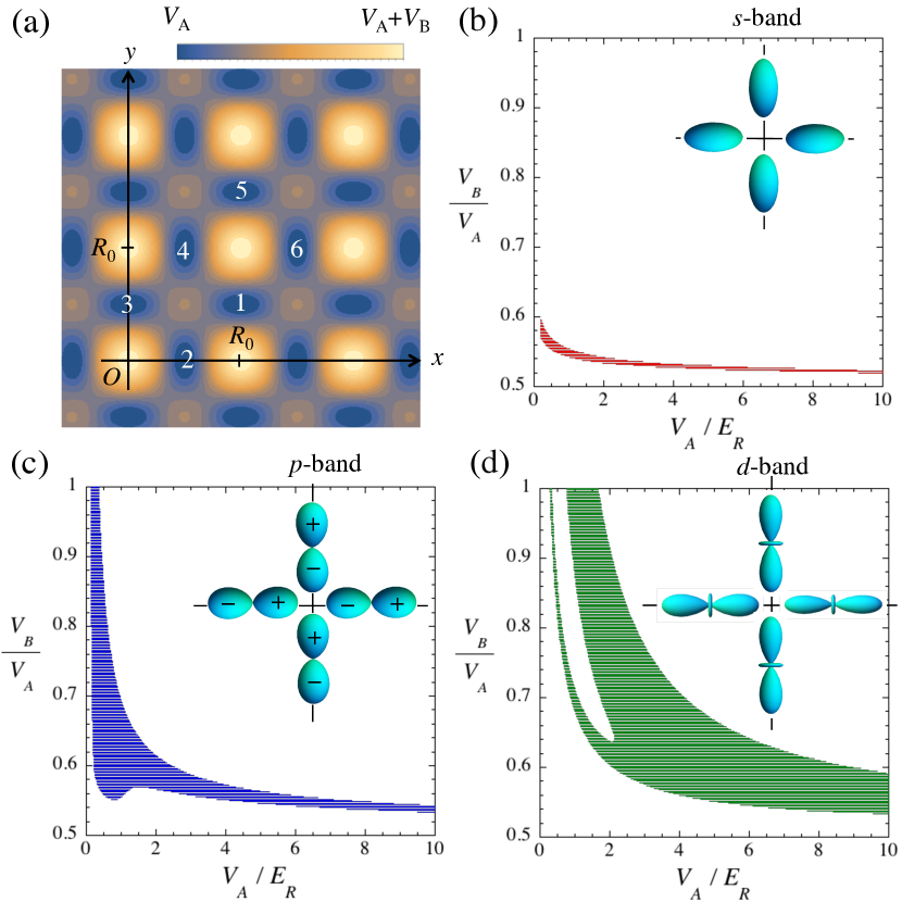
Figure 3: Method A to realize the value of $V_{ab}$ in Table 1 using excited bands of an optical lattice. (a) The profile of the optical lattice of Eq. (10) for $V_{\mathrm{A}}=V_{\mathrm{B}}$. The minima of the lattice are located at $(x,y)=R_{0}(m_{x},m_{y}+1/2)$ for the horizontal links and $(x,y)=R_{0}(m_{x}+1/2,m_{y})$ for the vertical links ($m_{x,y}$: integers), where $R_{0}=\pi/k$ is the lattice constant. The panels (b)-(d) show the domains (colored region) that satisfy the approximated condition for the overlap integral $0.95<O_{12}/O_{13}<1.05$ and $O_{15}/O_{12}\leq 0.1$ in the $V_{\mathrm{A}}/E_{R}$-$V_{\mathrm{B}}/V_{\mathrm{A}}$ plane for $s$-, $p$-, and $d$-orbitals, respectively. For $p$-, and $d$-orbitals, the domains bifurcate due to the radial peak structure of the Wannier function (see Appendix B).

The intersite density-density interaction is proportional to the overlap integral $O_{ab}=\int d\mathbf{r}|w_{a}|^{2}|w_{b}|^{2}$, where $w_{a}$ is the Wannier function at the link $(r,a)$ and we assume a negligibly small DDI. For the horizontal links, by approximating a minimum of the optical lattice as a quadratic form $m\omega_{\mathrm{ho}}^{2}(\alpha^{2}x^{2}+y^{2})/2$, $w_{a}$ can be represented by the harmonic oscillator basis $\Phi_{\mathbf{n}}(\mathbf{r})$, where $\hbar\omega_{\mathrm{ho}}=2\sqrt{E_{R}(V_{\mathrm{A}}+2V_{\mathrm{B}})}$ with the recoil energy $E_{R}=\hbar^{2}k^{2}/2m$ of the optical lattice and $\alpha=\sqrt{(2V_{\mathrm{B}}-V_{\mathrm{A}})/(2V_{\mathrm{B}}+V_{\mathrm{A}})}$. The band index takes $\mathbf{n}=(0,0)$, $(1,0)$, and $(2,0)$ for the $s$-, $p$-, and $d$-orbitals. For the vertical links, the role of $(x,y)$ is just exchanged by $(y,x)$.

The conditions in Table 1 read $O_{12}\approx O_{13}\gg O_{15}$. Figures 3(b)-(d) represent the parameter domain satisfying this condition with respect to $V_{\mathrm{A}}$ and $V_{\mathrm{B}}/V_{\mathrm{A}}$, where the amplitudes $V_{\mathrm{A}}$ and $V_{\mathrm{B}}$ of the optical lattice are precisely tunable parameters. Because of the characteristics of the potential Eq. (10), we can have significant overlap of the Wannier functions even for the high potential height such as $V_{\mathrm{A,B}}=100E_{R}$ for $V_{\mathrm{B}}/V_{\mathrm{A}}\geq 0.5$; see Appendix B for more details. For the $s$-orbitals the domain is limited to a narrow region ($V_{\mathrm{B}}\sim 0.55V_{\mathrm{A}}$) of the parameter space. Using the $p$- or $d$- orbitals allows us to get the condition of Table 1 more easily in the experimentally feasible condition. When the excited orbitals are used, we have significant hopping amplitudes $J_{ab}$ not only for the NN ($J$) but also the 1st half of NNN $(J^{\prime})$; the 2nd half of NNN ($J^{\prime\prime}$) is small because of higher potential height between the link of group (iii) as seen in Fig. 3(a).

Finally, we admit that, for actual parameter estimation, one should also try other more realistic Wannier functions such as $\sim x^{c}\exp(-h|x|)$ He , although the qualitative feature captured here needs no modifications.

IV.2 Method B: Using dipolar atoms in a multilayer optical lattice

The idea for the second method is to introduce new subsidiary 2D lattices and treat the DDI between atoms in the original 2D lattice and atoms in the subsidiary lattices by the second-order perturbation theory to obtain $V_{ab}$ effectively. For illustrative purpose, we explicitly describe the idea by using a triple-layer system consisting of three 2D square optical lattices (layer L_A, L_B, L_C) as seen in Fig. 4(a). Here, we neglect the contribution of short-range interaction for the intersite interaction. The scheme may be reduced to a double-layer system by approaching the distance between two layers, e.g. L_A and L_B, to zero, which is discussed for realistic parameter estimation at the end of Appendix C.

The boson system on the layer L_A (we call them A-bosons) is a playground of the (2+1)D U(1) GH model, which is sandwiched by B-bosons on L_B and C-bosons on L_C. The B- and C-bosons are trapped in deep optical lattices with negligible hopping. Each layer has different basis vectors of the lattice structure as shown in Fig. 4(b) and (c). Each species of bosons is assumed to have a dipole, perpendicular to the plane of the layer. By treating the DDI between A-boson and B-boson as a perturbation, the second-order perturbation theory generates an effective intersite interaction between the A-bosons. So is the DDI between A- and C-bosons, which generates another intersite interactions between the A-bosons. These two kinds of interactions may be tuned to realize $V_{ab}$ as given in Table 1. We omit the DDI between the B- and C-bosons because of the large separation.

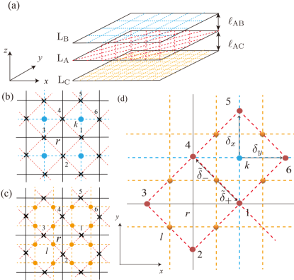
Figure 4: (a) The structure of a triple-layer 2D optical lattice. The LGT is simulated on the lattice of black solid lines. The layers are separated by distance $\ell_{\mathrm{AB}}$ and $\ell_{\mathrm{AC}}$. The panels (b) and (c) show the projective mapping of L_A (red lines) and L_B (blue lines), and L_A and L_C (orange lines), respectively. The panel (d) shows the unit cell of the projective mapping of the all layers. The site label of L_A and L_C are denoted as $k$ and $l$, respectively. For the layers L_B and L_A, we take the NN DDI between atoms on the sites $k$ in L_B and $k\pm\delta_{x}(\delta_{y})$ in L_A into account. For L_C and L_A, we take the NN DDI between atoms on the sites $l$ in L_C and $l+\tilde{\delta}_{+}(\tilde{\delta}_{-})$ in L_A into account.

Let us focus on Fig. 4(d). When one projects the sites of L_B onto L_A, their image locates on the center of each plaquette of the L_A lattice. Similarly, the image of sites of L_C locates on the middle of NN pairs of the L_A sites. In L_A, the A-bosons at different sites have the repulsive DDI. Furthermore, the A- and B(C)-bosons are coupled through the NN attractive DDI given by

$$H_{{\rm A}{\rm B}} =V_{{\rm A}{\rm B}}\sum_{k,\delta}\rho_{A,k+\delta}n_{B,k},$$

$$H_{{\rm A}{\rm C}} =V_{{\rm A}{\rm C}}\sum_{l,\tilde{\delta}}\rho_{{\rm A},l+\tilde{\delta}}n_{{\rm C},l},$$ (11)

where $\rho_{\mathrm{A},k}$ and $n_{\mathrm{B(C)},k}$ are boson densities at the site $k$ and $V_{{\rm A}{\rm B}({\rm C})}<0$ is the DDI, which is tunable by controlling the interlayer separation. Our strategy is to trace out B- and C-bosons to get the effective attractive intersite interactions between the A-bosons themselves. According to the usual second-order perturbation theory with $H_{{\rm A}{\rm B}({\rm C})}$ as perturbation, the effective attractive interaction between A-bosons may be estimated as $\sim-V^{2}_{{\rm A}{\rm B}}\sum_{k,\delta,\delta^{\prime}}\rho_{{\rm A},k+\delta}\rho_{{\rm A},k+\delta^{\prime}}$ and $-V^{2}_{{\rm A}{\rm C}}\sum_{l,\tilde{\delta}}\rho_{{\rm A},l+\tilde{\delta}}\rho_{{\rm A},l-\tilde{\delta}}$. They are due to density fluctuations of B- and C-bosons, respectively. The former term contributes a constant to $V_{ab}$ for (a,b) of the groups (i,iii) of Table 1, while the latter contributes a constant only for the group (i). Then one may fulfill the condition of $V_{ab}$ in Table 1. The detailed calculation of the effective interaction and the experimental feasibility are described in Appendix C. Although there is a small contribution of long-range interaction beyond the NNN links due to the power-law tail of $r^{3}$, this correction may suppress the density fluctuation and result in the enhancement of the confinement phase.

V conclusion and outlook

In conclusion, realization of the quantum simulator of the U(1) lattice-gauge Higgs model provides a significant innovation to tackle unresolved problems such as inflation universe, being possible to be constructed by the cold-atomic architecture. The phase structure of the atomic simulators may be explored by the non-equilibrium dynamics, where the electric flux dynamics can be observed from the behavior of the density fluctuation. We proposed two experimentally feasible schemes (Method A and B) to respect the constraint of Gauss’s law and locality of the gauge interaction in the atomic simulators.

Many works have been devoted to the dynamical properties of phase defects, namely quantized vortices, by analyzing the GP equation Pethicksimsh . In terms of the gauge theory, these phase defects correspond to the magnetic fluxes. Our work focuses on the density fluxes, corresponding to electric fluxes, whose dynamics are under constraint by the Gauss’s law. Such a density flux in the GP model has not been discussed before and this point of view could open the door for new avenue of the GP dynamics, such as dynamical features of various configurations of an electric flux or many fluxes. These non-equilibrium dynamics are interesting themselves, although they could also give references as a guide not only to the atomic simulator experiments but also to the LGT. The dynamical equations can be derived and give some insights for various models of the LGT.

The other problems for the future study includes the clarification of the global phase diagram of Eq. (3) for the general sets of parameters and of how to implement the general terms in Eq. (3) experimentally. It has been proposed in Ref. Kasamatsu that the Higgs coupling ($c_{1i}$-term) in the spatial dimension can be implemented by using an idea of Ref. Recati . An idea to generate the spatial plaquette ($c_{2ij}$-) term is discussed in Ref. Buchler . There is still insufficient discussion on how to combine these schemes toward the quantum simulation of the full GH model, which is a subject for future study. Fine tuning of the intersite density-density interaction is also an important task, and we believe that the method in Sec. IV.1 is the most feasible scheme in actual experiments. Our method in Sec. IV.2 provides a new scheme for tuning the intersite atom-atom interactions, and more elaborated discussion using concrete atomic species, optical lattice structures, etc., remains to be studied. All of these issues will be reported in future publications.

Appendix A Phase structure of the U(1) GH model

Let us explain the phase structure of the gauge-Higgs model defined by Eq. (3) with asymmetric couplings $c_{1\mu},c_{2\mu\nu}$ given by Eq. (4). First, we note that the (2+1)D version of the standard 4D U(1) Higgs gauge theory KK-complementarity , which is considered in HEP and has the symmetric couplings ($c_{1\mu}=c_{1}\geq 0,c_{2\mu\nu}=c_{2}\geq 0,c_{3,4,5}=0$ in Eq. (3)), is always in the confinement phase KK-Polyakon , in which the phase $\theta_{x,\mu}$ is unstable by strong fluctuation. In our model, inclusion of sufficient $c_{3}$ in addition to the asymmetric couplings $c_{1\mu}$ and $c_{2\mu\nu}$ lets the system enter into the “Higgs” phase, where both $\theta_{x,\mu}$ and $\varphi_{x}$ are stable [see Fig. 5].

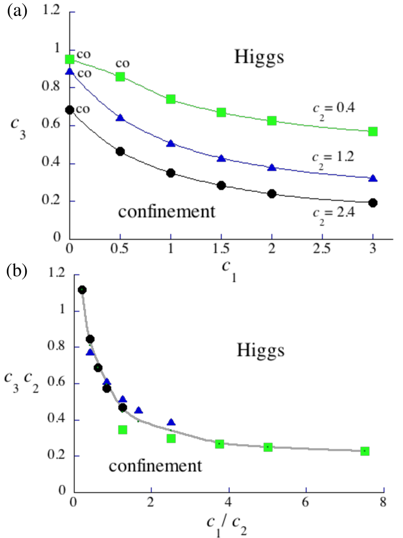
Figure 5: Phase diagram of the (2+1)D U(1) lattice GH model of Eq. (3) with asymmetric couplings $c_{1\mu}$ and $c_{2\mu\nu}$ given by Eq. (4) and $c_{4}=c_{5}=0$. (a) Three curves connect transition points in the $c_{1}$-$c_{3}$ plane for $c_{2}=0.4,1.2,2.4$ from above, which separate the Higgs phase (above) and the confinement phase (below). The transition points are located at the peak of $C$ as a function of $c_{3}$ for fixed $c_{1}$. They are (i) second-order (no marks) where the peak of $C$ develops as the size $L$ increases and $U$ exhibits no hysteresis or (ii) cross-over or Kosterlitz-Thouless transition (both marked with co) where the peak does not develop. (b) The transition points on (a) are arranged in the $(c_{1}/c_{2})-(c_{3}\cdot c_{2})$ plane ($\gamma^{2}V_{0}^{\prime}-2J\rho_{0}/V_{0}^{\prime}$ plane) . They almost sit on a single curve (gray line) (See the comment right after Eq. (5)).

To identify the location of the transitions, we measure the internal energy $U=\langle A\rangle$ and the specific heat $C=\langle A^{2}\rangle-\langle A\rangle^{2}$ by using the standard Metropolis algorithm in Monte Carlo (MC) simulation with the periodic boundary condition for the cubic lattice of size $V=L^{3}$ with $L$ up to 40. The typical number of sweeps is $100000+10000\times 10$, where the first number is for thermalization and the second one is for measurement. The errors of $U$ and $C$ are estimated by the standard deviation over 10 samples. Acceptance ratios in updating variables are controlled to be $0.6\sim 0.8$.

Explicitly, we confine ourselves to the case $c_{4}=c_{5}=0$ and obtain the phase diagram in the $c_{1}-c_{3}$ plane for several values of $c_{2}$. The result is presented in Fig. 5. There are two phases: the Higgs phase in the large $c_{3}$ region (upper region) and the confinement phase in the small $c_{3}$ region (lower region). The confinement-Higgs transition here should correspond to various phase transitions such as the superconducting transition, the mass generation in the standard model, and the believed one to take place in the early universe inflation1 ; inflation2 . In contrast to the phase diagram of the (3+1)D model for $c_{4}=c_{5}=0,c_{1}=c_{3}$, and $c_{2}\geq 0$ Kasamatsu , the Coulomb phase is missing due to the low dimensionality.

To understand Fig. 5, let us consider some limiting cases. First, after choosing the unitary gauge $\phi_{x}=1$, let us consider the limit $c_{1}\to\infty$. Then the $c_{1}$ term makes $\theta_{x,0}=0$ [mod(2$\pi$)], and the action becomes

$$A_{\rm c_{1}=\infty} = c_{2}\sum_{x}\sum_{i=1}^{2}\cos(\theta_{x+0,i}-\theta_{x,i})$$ (12)

$$+ c_{3}\sum_{x}\Big{[}\cos(\theta_{x,1}-\theta_{x,2})+\cos(\theta_{x,1}+\theta_{x+1,2})$$

$$+ \cos(\theta_{x+1,2}-\theta_{x+2,1})+\cos(\theta_{x,2}+\theta_{x+2,1})\Big{]},$$

up to constant. This is viewed as a 3D XY spin model with asymmetric couplings, where $\theta_{x,i}\ (i=1,2)$ on the link $(x,x+i)$ is the XY spin angle $\tilde{\theta}_{\tilde{x}}$. In fact, the $c_{3}$ term is their NN coupling in the 12 plane and the $c_{2}$ term is their NN coupling along the $\mu=0$ axis. The region of sufficiently large $c_{2}$ and $c_{3}$ is the ordered phase of this XY spins, and corresponds to the Higgs phase with small gauge-field ($\theta_{x,\mu}$) fluctuations. As a check of Fig. 5, let us consider the case $c_{2}=c_{3}$ of Eq. (12), which reduces to the symmetric 3D XY spin model of $A_{\rm 3DXY}=c_{\rm XY}\sum_{\tilde{x},\mu}\cos(\tilde{\theta}_{\tilde{x}+\mu}-\tilde{\theta}_{\tilde{x}})$. It is known to have a genuine second-order phase transition at $c_{\rm XY}\simeq 0.45$. Therefore the transition line in Fig. 5 (b) should approach to $c_{2}\cdot c_{3}\to 0.45^{2}\simeq 0.20$ as $c_{1}/c_{2}\to\infty$ as it shows.

Next, let us consider the case $c_{2}=0$. Then, each variable $\theta_{x,0}$ appears only through the $c_{1}$ term without couplings to other variables (we take the unitary gauge as before). Then the dynamics is controlled by the $c_{3}$ term. Again, this term is viewed as the energy of the XY spins $\theta_{xi}\ (i=1,2)$. However they have no coupling along the $\mu=0$ direction, and therefore the system is a collection of decoupled 2D XY spin models. 2D XY spin model is known to exhibit Kosterlitz-Thouless (KT) transition which is infinitely continuous. Thus, although it is not drawn in Fig. 5, there should be added a horizontal line (independent of $c_{1}$) for $c_{2}=0$ consisting of a collections of KT transitions at around $c_{3}\sim 0.96$. We understand that the crossover points appearing in the smaller $c_{1}$ part in each curve for three $c_{2}$ drawn in Fig. 5 are the remnants of these KT transitions. They have a chance to be a genuine KT transition, although we called them crossover here. Another support of this interpretation is to consider the case $c_{1}=0$. Then there is no source term for $\theta_{x,0}$ and $\theta_{x,0}$ should determine their dynamics only through the $c_{2}$ term. Thus, even $\theta_{x,i}$ could be set constant with no fluctuations, $\theta_{x,0}$ has the NN coupling in each 12 plane. However, two dimensions is not enough to stabilize $\theta_{x,0}$. In turn, the $c_{2}$ term is not enough to sustain the coupling between $\theta_{x,i}$ along the $\mu=0$ direction. The dynamics of $\theta_{x,i}$ is essentially from the $c_{3}$ term, which is the 2D XY model as explained. Therefore, the transition, if any, for $c_{1}=0$ may be a KT transition. No genuine second-order one is possible.

The last case is $c_{2}=\infty$. Then $\theta_{x,\mu}$ is frozen to be a pure gauge configuration, $\theta_{x,\mu}=\lambda_{x+\mu}-\lambda_{x}$. By plugging this into the $c_{1}$ and $c_{3}$ term, we obtain

$$A_{\rm c_{2}=\infty}=c_{1}\sum_{x}\cos(\lambda_{x+3}-\lambda_{x})$$

$$+2c_{3}\sum_{x}\Big{[}\cos(\lambda_{x+1}-\lambda_{x+2})+\cos(\lambda_{x}-\lambda_{x+1+2})\Big{]},$$ (13)

which belongs again to the class of 3D XY spin models, where $\lambda_{x}$ is the XY spin angles on the site $x$. So we should have a second-order transition at $c_{2}=\infty$ as long as both $c_{1}$ and $c_{3}$ are nonvanishing. This is consistent with Fig. 5.

Let us finally comment on the transition line of Fig. 5(b) and the boundaries of Fig. 2(a) calculated by dynamical simulation in Sec. III. Their behaviors in the $(c_{1}/c_{2})$-$(c_{3}\cdot c_{2})$ plane are qualitatively consistent but different in quantitative comparison. We understand that there are no inconsistency in these results because the two methods, MC and GP, are different in nature: MC is static and GP is dynamical, they treat fluctuations in contrasting manners, and especially, the dynamical simulations necessarily exhibit various properties of the system according to their setup and probes, etc. This certainly motivates exact quantum and dynamical simulation of the BH model in experiments.

Appendix B Calculation of overlap integrals

In this section, we describe the calculation of the overlap integrals discussed in Sec. III A. For the horizontal links of the potential $V_{\mathrm{OL}}$ of Eq. (10), the minimum is approximated by the harmonic oscillator $V_{hx}=m\omega_{\mathrm{ho}}^{2}(\alpha^{2}x^{2}+y^{2})/2$. The basis function of $V_{hx}$ is given by

$$\Phi_{\mathbf{n}}(\sqrt{\alpha}x,y)=A_{\mathbf{n}}H_{n_{x}}\left(\sqrt{\alpha}\frac{x}{a_{\mathrm{ho}}}\right)H_{n_{y}}\left(\frac{y}{a_{\mathrm{ho}}}\right)e^{-(\alpha x^{2}+y^{2})/2a_{\mathrm{ho}}^{2}},$$ (14)

where $H_{n}$ is the Hermite polynomial, $A_{\mathbf{n}}$ the normalization factor, and $a_{\mathrm{ho}}=\sqrt{\hbar/m\omega_{\mathrm{ho}}}$ the harmonic oscillator length

The $s$, $p$, and $d$ orbitals for these links correspond to $\mathbf{n}=(n_{x},n_{y})=(0,0)$, $(1,0)$, and $(2,0)$. As the Wannier function $w_{a}(\mathbf{r})$ at the link $(r,a)$, we use $\Phi_{\mathbf{n}}$ with $(x,y)$ measured from the center of the link. For the vertical links, the minimum is also approximated as $V_{hy}=m\omega_{\mathrm{ho}}^{2}(x^{2}+\alpha^{2}y^{2})/2$ and the basis function is $\Phi_{\mathbf{n}}(x,\sqrt{\alpha}y)=A_{n}H_{n_{x}}(x/a_{\mathrm{ho}})H_{n_{y}}(\sqrt{\alpha}y/a_{\mathrm{ho}})e^{-(x^{2}+\alpha y^{2})/2a_{\mathrm{ho}}^{2}}$. The $s$, $p$, and $d$ orbitals for these links correspond to $\mathbf{n}=(n_{x},n_{y})=(0,0)$, $(0,1)$, and $(0,2)$. Then, the Wannier functions $w_{a}(\mathbf{r})$, relevant to the following calculations, are given as follows;

$$w_{1}(\mathbf{r}) =\Phi_{\mathbf{n}}(\sqrt{\alpha}R_{0}(\tilde{x}-1/2),R_{0}\tilde{y}),$$

$$w_{2}(\mathbf{r}) =\Phi_{\mathbf{n}}(R_{0}\tilde{x},\sqrt{\alpha}R_{0}(\tilde{y}+1/2)),$$

$$w_{3}(\mathbf{r}) =\Phi_{\mathbf{n}}(\sqrt{\alpha}R_{0}(\tilde{x}+1/2),R_{0}\tilde{y}),$$

$$w_{5}(\mathbf{r}) =\Phi_{\mathbf{n}}(\sqrt{\alpha}R_{0}(\tilde{x}-1/2),R_{0}(\tilde{y}-1),$$ (15)

where $R_{0}$ represents the lattice spacing and we shift the origin of the coordinate to $(R_{0}/2,R_{0}/2)$ of Fig. 3(a). The length scale of the coordinate is normalized by $R_{0}$ and the dimensionless coordinates are denoted by putting tildes.

The intersite interaction strength $V_{ab}$ is proportional to the overlap integrals $O_{ab}=\int d\mathbf{r}|w_{a}|^{2}|w_{b}|^{2}$. It is sufficient to calculate only the integrals for the link pairs $(a,b)=(1,2)$, $(1,3)$, and $(1,5)$, because $O_{12}=O_{23}=O_{34}=O_{41}$, $O_{13}=O_{24}$, and $O_{15}=O_{26}$ due to the lattice symmetry.

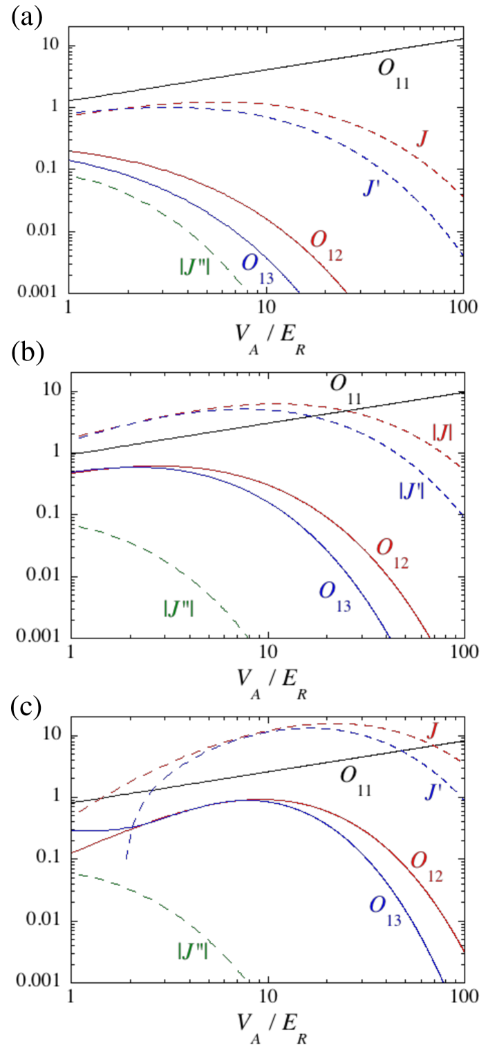
Figure 6: Overlap integral $O_{ab}$ and hopping integrals $J$, $J^{\prime}$, and $J^{\prime\prime}$ as a function of $V_{\mathrm{A}}/E_{R}$ for $V_{\mathrm{B}}/V_{\mathrm{A}}=0.6$. The panels (a), (b), and (c) corresponds to the cases of $s$-, $p$- , and $d$-wave orbitals. Using $O_{ab}$, the density-density interaction is written by $V_{ab}/E_{R}=(8a/\pi l_{z})O_{ab}$ with the $s$-wave scattering length $a$ and the typical length scale $l_{z}$ along the $z$-direction. The hopping is also normalized by $E_{R}$ and its negative value is plotted by the absolute value. In the $p$-orbital case, $J_{12}(=J)$ and $J_{13}(=J^{\prime})$ become negative, but there is no frustration because of $J_{23},J_{41}>0$ and $J_{34},J_{24}<0$.

The typical results of the overlap integrals for the three orbitals are shown in Fig. 6 for $V_{\mathrm{B}}/V_{\mathrm{A}}=0.6$ as a function of $V_{\mathrm{A}}$. We also show the integral for on-site contribution $O_{11}=\int d\mathbf{r}|w_{a}|^{4}$ and the hopping integrals $J=\int d\mathbf{r}w_{1}(-\hbar^{2}\nabla^{2}/2m+V_{\mathrm{OL}})w_{2}$, $J^{\prime}=\int d\mathbf{r}w_{1}(-\hbar^{2}\nabla^{2}/2m+V_{\mathrm{OL}})w_{3}$, and $J^{\prime\prime}=\int d\mathbf{r}w_{1}(-\hbar^{2}\nabla^{2}/2m+V_{\mathrm{OL}})w_{5}$. In any case, $O_{11}$ is monotonically increased with $V_{\mathrm{A}}$, and $J^{\prime\prime}$ and $O_{15}$ (not seen in Fig. 6) are negligibly small. In the case of the $s$-orbital, $O_{12}$ and $O_{13}$ are also monotonically decreasing functions, so that the range satisfying $O_{12}\approx O_{13}$ is only limited by a narrow range or a point with respect to $V_{\mathrm{A}}$. On the other hand, for the $p$- and $d$-orbitals $O_{12}$ and $O_{13}$ changes non-monotonically because of the node structure and the extended amplitude profile of the wave functions. This fact extends the range of $O_{12}\approx O_{13}$ as seen in Fig. 6(b) and (c).

Note that the hopping integrals $J$ and $J^{\prime}$ are of ${\cal O}(1)$ even for $V_{\mathrm{A}}=100E_{R}$. This is because the energy barrier between links of group (i) and (ii) in Table LABEL:vab is the sub-maximum with the height $2V_{\mathrm{B}}-V_{\mathrm{A}}$ at $(R_{0}/2,R_{0}/2)$ in Fig. 3(a). Since, the value of $J(J^{\prime})$ is bigger than that of $O_{12(13)}$ by two orders of magnitude, one needs to increase considerably the $s$-wave scattering length via a Feshbach resonance to get the exact Gauss’s law constraint, namely, $V_{ab}\gg J$.

Appendix C Effective intersite interaction in the triple-layer system of Sec. IV.2

In this section, we apply the second-order perturbation theory to the triple-layer system in Sec. IV.2 to derive the effective intersite interaction of A-bosons, and estimate the possible values of involved parameters to realize $V_{ab}$ of Table 1. After that, we briefly explain a double-layer system in which magnitude of the intersite interaction of A-bosons is controlled in a similar way.

We first confine ourselves to the subsystem of the A- and B-bosons (two layers L_A and L_B) which has the NN DDI, $H_{{\rm A}{\rm B}}$ of Eq. (11). It implies that the B-boson on the site $k$ interacts with the four NN A-bosons on the sites $k\pm\delta_{x(y)}$ as seen in Fig. 4(d). $V_{{\rm A}{\rm B}}$ in $H_{{\rm A}{\rm B}}$ is expressed as

$$V_{{\rm A}{\rm B}} = \int d\mathbf{r}d\mathbf{r}^{\prime}U_{\mathrm{DD}}(\mathbf{r},\mathbf{r}^{\prime})|w_{{\rm A}}(\mathbf{r})|^{2}|w_{{\rm B}}(\mathbf{r}^{\prime})|^{2},$$

$$U_{\mathrm{DD}}(\textbf{r},\textbf{r}^{\prime}) = \frac{C}{4\pi|\textbf{r}-\textbf{r}^{\prime}|^{3}}\biggl{(}1-\frac{3\ell^{2}_{\mathrm{AB}}}{|\textbf{r}-\textbf{r}^{\prime}|^{2}}\biggr{)},$$ (16)

where $\mathbf{r}(\mathbf{r}^{\prime})$ is the position of A(B)-boson, $w_{{\rm A}({\rm B})}(\mathbf{r})$ is their Wannier function, and $C=\mu_{0}\tilde{\mu}_{{\rm A}}\tilde{\mu}_{{\rm B}}$; $\mu_{0}$ is the magnetic permeability of the vacuum and $\tilde{\mu}_{{\rm A}({\rm B})}$ is the magnetic moment of A(B)-atoms.

We assume that the B-bosons of L_B have a chemical potential $\mu_{{\rm B}}$($>0)$, a negligibly small NN hopping amplitude due to a deep trapping potential, an on-site repulsion $U_{\rm B}(>0)$, and the NN DDI with A-bosons $V_{{\rm A}{\rm B}}$. One may forget the DDI between B-bosons, because it is a constant due to negligible NN hopping. Then, the Hamiltonian $\hat{H}_{\rm B}$ and the partition function $Z_{{\rm B}}={\rm Tr}\exp(-\beta\hat{H}_{\rm B})$ for the subsystem of B-bosons are written by using the B-boson density operator $\hat{n}_{k}$ at the site $k$ as

$$\hat{H}_{{\rm B}} =\sum_{k}\Bigl{[}-\mu_{{\rm B}}\hat{n}_{k}+U_{{\rm B}}\hat{n}_{k}(\hat{n}_{k}-1)+V_{{\rm A}{\rm B}}\!\!\sum_{\delta=\pm\delta_{x,y}}\!\!\hat{n}_{k}\hat{\rho}_{k+\delta}\Bigr{]},$$

$$Z_{{\rm B}} =\prod_{k}z_{{\rm B},k},\ z_{{\rm B},k}\!=\!\sum_{n=0}^{\infty}\exp\biggl{[}-\beta\bigl{(}E_{n}+nV_{{\rm A}{\rm B}}\sum_{\delta}\hat{\rho}_{k+\delta})\bigg{]},$$

$$E_{n} =-\mu_{\rm B}n+U_{\rm B}n(n-1).$$ (17)

By assuming $\mu_{{\rm B}},U_{{\rm B}}\gg V_{{\rm A}{\rm B}}$, we expand $z_{{\rm B},k}$ up to $O(V_{{\rm A}{\rm B}}^{2})$,

$$z_{{\rm B},k} =\sum_{n=0}^{\infty}e^{-\beta E_{n}}\biggl{[}1-nW_{k}+\frac{1}{2}n^{2}(W_{k})^{2}\cdots\biggr{]}$$

$$=F_{0}\left[1-\frac{F_{1}}{F_{0}}W_{k}+\frac{1}{2}\frac{F_{2}}{F_{0}}(W_{k})^{2}\cdots\right],$$

$$W_{k} =\beta V_{{\rm A}{\rm B}}\sum_{\delta}\hat{\rho}_{k+\delta},\hskip 8.53581ptF_{m}\equiv\sum_{n=0}^{\infty}n^{m}e^{-\beta E_{n}}.$$ (18)

Then we have

$$Z_{{\rm B}}=(F_{0})^{L^{2}}\exp\biggl{\{}\sum_{k}\Bigl{[}\langle-n\rangle_{0}W_{k}+\frac{1}{2}(\Delta n)^{2}(W_{k})^{2}+\cdots\Bigr{]}\biggr{\}},$$

$$\langle n^{m}\rangle_{0}\equiv\frac{F_{m}}{F_{0}},\hskip 14.22636pt(\Delta n)^{2}\equiv\langle n^{2}\rangle_{0}-\langle n\rangle_{0}^{2}.$$ (19)

The first-order terms $\propto W_{k}$ are renormalized to the chemical potential of A-bosons and the second-order terms define the effective density-density interaction Hamiltonian $\hat{H}_{{\rm A}{\rm B}{\rm A}}$ of A-bosons induced by B-boson density fluctuation $(\Delta n)^{2}$,

$$\hat{H}_{{\rm A}{\rm B}{\rm A}}=-\frac{\beta}{2}(\Delta n)^{2}V_{\mathrm{AB}}^{2}\sum_{k}\sum_{\delta,\delta^{\prime}}\hat{\rho}_{k,\delta}\hat{\rho}_{k,\delta^{\prime}}.$$ (20)

The DDI between A-atoms and C-atoms can be analyzed in the same way, and we obtain another effective density-density interaction for the A-bosons, $\hat{H}_{{\rm A}{\rm C}{\rm A}}=-(\beta/2)(\Delta n^{\prime})^{2}V^{2}_{{\rm A}{\rm C}}\sum_{l,\bar{\delta},\bar{\delta}^{\prime}}\hat{\rho}_{l+\bar{\delta}}\hat{\rho}_{l+\bar{\delta}^{\prime}},$ where $(\Delta n^{\prime})^{2}$ is obtained by replacing $\mu_{\rm B},U_{\rm B}$ by $\mu_{\rm C},U_{\rm C}$ in $(\Delta n)^{2}$.

The sum $\hat{H}_{{\rm A}{\rm B}{\rm A}}+\hat{H}_{{\rm A}{\rm C}{\rm A}}$ contributes to the coefficients $V_{ab}$ of the intersite density-density interactions for A-bosons as follows;

$${\rm For\ NN\ links\ (group\ (i)\ in\ Table~{}\ref{paratable})},$$

$$V_{ab}=V-\beta(\Delta n)^{2}V^{2}_{{\rm A}{\rm B}}-\beta(\Delta n^{\prime})^{2}V^{2}_{{\rm A}{\rm C}},$$

$${\rm For\ NNN\ links},$$

$$V_{ab}=\left\{\begin{array}[]{ll}V^{\prime}&\ \mathrm{for\ group\ (ii)}\\ V^{\prime}-\beta(\Delta n)^{2}V^{2}_{{\rm A}{\rm B}}&\ \mathrm{for\ group\ (iii)},\end{array}\right.$$ (23)

where $V$ and $V^{\prime}$ are the direct DDI for NN and NNN link pairs, respectively. The condition for $V_{ab}$ in Table 1 can be established by adjusting two inter-layer distances $\ell_{{\rm A}{\rm B}}$ and $\ell_{{\rm A}{\rm C}}$ and density fluctuations $(\Delta n)^{2}(\mu_{\rm B},V_{\rm B},\beta)$ and $(\Delta n^{\prime})^{2}(\mu_{\rm C},V_{\rm C},\beta)$ as

$$\beta(\Delta n^{\prime})^{2}V^{2}_{{\rm A}{\rm C}}=V-2V^{\prime},$$

$$\beta(\Delta n)^{2}V^{2}_{{\rm A}{\rm B}}=V^{\prime}(=\gamma^{-2}).$$ (24)

Let us present some brief account for an example and estimation of the experimental parameters that satisfy the tuning relations Eq.(24). We shall report detailed discussion on this example and related topics in a future publication.

For bosons loaded in each layer we consider ⁵²Cr atoms Griesmaier as A bosons, ⁸⁷Rb atoms as B bosons, and ¹⁶⁸Er atoms Aikawa as C bosons. They have the permanent magnetic moments $6\mu_{\rm BM},\mu_{\rm BM}$, and $7\mu_{\rm BM}$ ($\mu_{\rm BM}$ is a Bohr magneton), respectively. Then we are interested in the effective double-layer system, which is obtained from the triple-layer system explained above by choosing $\ell_{\rm AB}=0$. The reason for using the double-layer system is to make the intersite interaction as large as possible because the magnetic moment of ⁸⁷Rb atom is small.

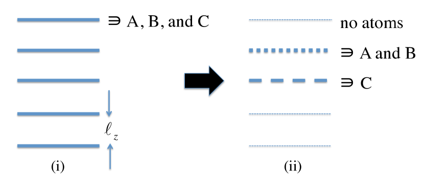
Figure 7: Making a double-layer system with three kinds of dipole atoms, A, B and C. (i) We prepare a 3D optical lattice. Each $x$-$y$ plane is separated by the distance $\ell_{z}$ and has the 2D lattice structure of the superposition of the three layers L_A,B,C shown in Fig. 3. Then we supply the A,B,C atoms so that every $x-y$ layer is viewed as the triple-layer system of Fig. 3 with $\ell_{\rm AB}=\ell_{\rm AC}=0$. (ii) We blow almost all the atoms off in such a way that only the A and B atoms in one $x-y$ layer and the C atoms in the next layer left. The resulting double-layer system is viewed as the triple-layer system of Fig. 3 with $\ell_{\rm AB}=0$ and $\ell_{\rm AC}=\ell_{z}$.

The method to make such a double-layer system is sketched in Fig. 7. First, one prepares the 3D layer system as shown in Fig. 7(i) by emitting three standing waves with the wavelengths satisfying $2\lambda_{1}=\sqrt{2}\lambda_{2}=\lambda_{3}$ (e.g., $\lambda_{1}=410$nm, $\lambda_{2}=580$nm and $\lambda_{3}=820$nm) in eight appropriate directions in the $x$-$y$ plane, each being separated by 45 degrees. In addition, we emit another standing-wave laser in the $z$-direction with the wavelength $\lambda_{z}$ to establish the 3D structure. Because ⁵²Cr,⁸⁷Rb and ¹⁶⁸Er exhibit the specific strong absorptions of photon with wave length 425nm, 780nm and 401nm, respectively, above standing waves load these atoms to the sites of corresponding layer L_A,B,C Bloch_RMP . This completes the step (i) in Fig. 7.

In the second step (ii) on Fig. 7, one needs to remove almost all the atoms except for those in two adjacent $x$-$y$ layers. This can be experimentally realized by using the technique of a position-dependent microwave transfer in a magnetic field gradient perpendicular to the layers Bloch_nat successively. This achieve to make an effective double-layer system with $\ell_{\rm AB}=0,\ell_{\rm AC}=\ell_{z}$.

Finally, let us estimate the parameters to satisfy the tuning relation Eq. (24). By making a straightforward calculation using DDI, we find that the following is a typical example of parameters :

$$V\sim\frac{36\mu_{0}\mu_{\rm BM}^{2}}{4\pi\lambda^{3}_{2}},\hskip 14.22636pt\ell_{\rm AC}=\ell_{z}\sim 580\ [\mathrm{nm}],$$

$$\beta\sim\frac{1}{2V},\hskip 14.22636ptU_{\rm B}\sim 0.3V,\hskip 14.22636pt\mu_{\rm B}\sim 2.5V,$$

$$U_{\rm C}\sim 1.3V,\hskip 14.22636pt\mu_{\rm C}\sim 2V.$$ (25)

The average densities per site are $\sim 560$ for B bosons and $\sim 8$ for C bosons. The ratio $|V_{\rm AB(C)}/\mu_{\rm B(C)}|$ is $\sim 0.192$($\sim 0.585$), which seems to validate the perturbation theory.

References

- (1) M. Lewenstein, A. Sanpera, and V. Ahufinger, Ultracold Atoms in Optical Lattices: Simulating Quantum Many-body Systems (Oxford: Oxford University Press, 2012).
- (2) K. Wilson, Phys. Rev. D 10, 2445 (1974).
- (3) J. B. Kogut, Rev. Mod. Phys. 51, 659 (1979).
- (4) U. -J. Wiese, Annalen der Physik 525, 777 (2013).
- (5) E. Zohar, J. I. Cirac, and B. Reznich, Phys. Rev. Lett. 109, 125302 (2012).
- (6) L. Tagliacozzo, A. Celi, A. Zamora, and M. Lewenstein, Ann. Phys. 330, 160 (2013).
- (7) D. Banerjee, M. Dalmonte, M. Müller, E. Rico, P. Stebler, U.-J. Wiese, and P. Zoller, Phys. Rev. Lett. 109, 175302 (2012).
- (8) E. Zohar, J. I. Cirac, and B. Reznich, Phys. Rev. Lett. 110, 055302 (2013).
- (9) E. Zohar, J. I. Cirac, and B. Reznich, Phys. Rev. Lett. 110, 125304 (2013).
- (10) D. Banerjee, M. Bögli, M. Dalmonte, E. Rico, P. Stebler, U.-J. Wiese, and P. Zoller, Phys. Rev. Lett. 110, 125303 (2013).
- (11) L. Tagliacozzo, A. Celi, P. Orland, M. W. Mitchell, and M. Lewenstein, Nat. Commun. 4, 2615 (2013).
- (12) D. Horn, Phys. Lett. B 100, 149 (1981).
- (13) P. Orland and D. Rohrlich, Nucl. Phys. B 338, 647 (1990).
- (14) S. Chandrasekharan and U.-J Wiese, Nucl. Phys. B 492, 455 (1997).
- (15) J. Kogut and L. Susskind, Phys. Rev. D 11, 395 (1975).
- (16) E. Zohar, J. I. Cirac, and B. Reznik Phys. Rev. A 88, 023617 (2013).
- (17) E. Zohar and B. Reznik, Phys. Rev. Lett. 107, 275301 (2011).
- (18) S. Tewari, V. W. Scarola, T. Senthil, and S. Das Sarma, Phys. Rev. Lett. 97, 200401 (2006).
- (19) K. Kasamatsu, I. Ichinose, and T. Matsui, Phys. Rev. Lett. 111, 115303 (2013).
- (20) E. Fradkin and S. H. Shenker, Phys. Rev. D 19, 3682 (1979).
- (21) K. Aoki, K. Sakakibara, I. Ichinose and T. Matsui, Phys. Rev. B 80, 144510 (2009).
- (22) A. H. Guth, Phys. Rev. D 23, 347 (1981).
- (23) E. Kolb and M. Turner, The Early Universe, (Boulder, CO: Westview Press, 1994).
- (24) J. Motruk and A. Mielke, J. Phys. A 45 (2012) 225206.
- (25) T. Lahaye, C. Menotti, L. Santos, M. Lewenstein, and T. Pfau, Rep. Prog. Phys. 72, 126401 (2009).
- (26) V. M. Scarola and S. Das Sarma, Phys. Rev. Lett. 95, 033003 (2005).
- (27) P. G. Kevrekidis, The Discrete Nonlinear Schrödinger Equation, (Berlin: Springer, 2009).
- (28) A. Reinhard, J. Riou, L. A. Zundel, D. S. Weiss, S. Li, A. M. Rey, and R. Hipolito, Phys. Rev. Lett. 110, 033001 (2013).
- (29) S. Wenzel, E. Bittner, W. Janke, A. M. J. Schakel, and A. Schiller, Phys. Rev. Lett. 95, 051601 (2005).
- (30) B. Yan, S. A. Moses, B. Gadway, J. P. Covey, K. R. A. Hazzard, A. M. Rey, D. S. Jin, and J. Ye, Nature(London) 501, 521 (2013).
- (31) A. de Paz, A. Sharma, A. Chotia, E. Maréchal, J. H. Huckans, P. Pedri, L. Santos, O. Gorceix, L. Vernac, and B. Laburthe-Tolra, Phys. Rev. Lett. 111, 185305 (2013).
- (32) A. V. Gorshkov, S. R. Manmana, G. Chen, E. Demler, M. D. Lukin, and A. M. Rey, Phys. Rev. A 84, 033619 (2011).
- (33) G. Möller and R. Moessner, Phys. Rev. Lett. 96, 237202 (2006).
- (34) A. W. Glaetzle, M. Dalmonte, R. Nath, I. Rousochatzakis, R. Moessner, and P. Zoller, Phys. Rev. X 4, 041037 (2014).
- (35) A. Macia, G. E. Astrakharchik, F. Mazzanti, S. Giorgini, J. Boronat, Phys. Rev. A 90, 043623 (2014).
- (36) T. Müller, S. Fölling, A. Widera, and I. Bloch, Phys. Rev. Lett. 99, 200405 (2007).
- (37) G. Wirth, M. Ölschläger, and A. Hemmerich, Nat. Phys. 7, 147 (2011).
- (38) M. Ölschläger, G. Wirth, and A. Hemmerich, Phys. Rev. Lett. 106, 015302 (2011).
- (39) L. He and D. Vanderbilt Phys. Rev. Lett. 86, 5341 (2001).
- (40) C. J. Pethick and H. Smith Bose-Einstein Condensation in Dilute Gases, 2nd ed., (Cambridge Univ. Press, Cambridge, 2008).
- (41) A. Recati, P. O. Fedichev, W. Zwerger, J. von Delft, and P. Zoller, Phys. Rev. Lett. 94, 040404 (2005).
- (42) H. P. Büchler, M. Hermele, S. D. Huber, M. P. A. Fisher, and P. Zoller, Phys. Rev. Lett. 95, 040402 (2005).
- (43) A. M. Polyakov, Phys. Lett. B 59, 82 (1975).
- (44) A. Griesmaier, J. Werner, S. Hensler, J. Stuhler, and T. Pfau, Phys. Rev. Lett. 94, 160401 (2005).
- (45) K. Aikawa, A. Frisch, M. Mark, S. Baier, A. Rietzler, R. Grimm, and F. Ferlaino, Phys. Rev. Lett. 108, 210401 (2012).
- (46) I. Bloch, J. Dalibard, and W. Zwerger, Rev. Mod. Phys. 80, 885 (2008).
- (47) J. F. Sherson, C. Weitenberg, M. Endres, M. Cheneau, I. Bloch and S. Kuhr, Nature. 467, 68-72 (2010).