Chemical abundance analysis of symbiotic giants – III. Metallicity and CNO abundance patterns in 24 southern systems

Abstract

The elemental abundances of symbiotic giants are essential to address the role of chemical composition in the evolution of symbiotic binaries, to map their parent population, and to trace their mass transfer history. However, the number of symbiotic giants with fairly well determined photospheric composition is still insufficient for statistical analyses. This is the third in a series of papers on the chemical composition of symbiotic giants determined from high resolution ($R$ $\sim$ 50000), near-infrared spectra. Here we present results for 24 S-type systems. Spectrum synthesis methods employing standard local thermal equilibrium analysis and atmosphere models were used to obtain photospheric abundances of CNO and elements around the iron peak (Fe, Ti, Ni, and Sc). Our analysis reveals metallicities distributed in a wide range from slightly supersolar ([Fe$/$H]$\sim+0.35$ dex) to significantly subsolar ([Fe$/$H]$\sim-0.8$ dex) but principally with near-solar and slightly subsolar metallicity ([Fe$/$H]$\sim-0.4$ to $-0.3$ dex). The enrichment in ¹⁴N isotope, found in all these objects, indicates that the giants have experienced the first dredge-up. This was confirmed in a number of objects by the low ¹²C/¹³C ratio (5–23). We found that the relative abundance of [Ti/Fe] is generally large in red symbiotic systems.

1 Introduction

Symbiotic stars are long-period binary systems consisting of two stars representing a late stage in stellar evolution: the cool primary and hot and luminous secondary (typically white dwarf albeit a neutron star has been found in a few cases) surrounded by an ionized nebula. Based on their near-infrared (IR) characteristics, symbiotic stars are divided into two main classes: S-type with normal red giant ($\sim$80 per cent), and D-type with Mira variable embedded in an optically thick dust shell ($\sim$20 per cent). A strong interaction between components is driven by mass loss from the cool donor that is partly accreted from the wind and$/$or via Roche lobe overflow (Podsiadlowski & Mohamed 2007; Mikołajewska 2012) on to the hot companion. In the past, when the present compact object underwent its red giant stage, mass had to be transferred in the opposite direction from this star to the star that is currently a red giant. That mass transfer episode should have left traces in the chemical composition of the red giant observed today. Indeed such chemical pollution has been detected in some red giant–white dwarf binary systems (Smith & Lambert, 1988).

Knowledge of the atmospheric chemical composition of symbiotic giants is of special significance as it can be used to track the mass exchange history as well as their population origin. However, at the moment reliable measurements of photospheric compositions exist for only 10 symbiotic systems with late-type (M) giants and about a dozen ‘yellow’, i.e. G or K giant, symbiotic systems. Prior to the current series of papers only four M giants in S-type symbiotic systems had been analysed in the literature: V2116 Oph (Hinkle et al., 2006), T CrB, RS Oph (Wallerstein et al., 2008), and CH Cyg (Schmidt et al., 2006). All of them had solar or nearly solar metallicities. The rarer symbiotic stars containing K-type giants are metal poor with s-process elements overabundant (Smith et al. 1996, 1997; Pereira, Smith & Cunha 1998; Pereira & Roig 2009) whereas those with G-type giants have solar metallicity and s-process enhancement (Smith, Pereira & Cunha 2001; Pereira, Smith & Cunha 2005).

Table 1: Journal of spectroscopic observations. Quadrature sums of the projected rotational velocities and microturbulence$\,{}^{a}$ $(V_{\mathrm{rot}}^{2}\sin^{2}{i}+\xi^{2}_{\mathrm{t}})^{0.5}$ shown have been obtained via cross-correlation technique (CCF) and from measurement of full width at half-maximum (FWHM) of $K$ band Ti i, Fe i, and Sc i absorption lines. Orbital phases have been calculated according to the referenced literature ephemeris. The full table with all 24 objects included is shown in the online Appendix A (Table 7).

	Id. num.b	Sp. region	Date	HJD (mid)	$(V_{\mathrm{rot}}^{2}\sin^{2}{i}+\xi^{2}_{\mathrm{t}})^{0.5}$		Orbital phasec
		band ($\lambda$[µm])	(dd.mm.yyyy)		CCF	FWHM
		$H$ ($\sim$1.56)	16.02.2003	245 2686.7409	6.08	–	0.30
BX Mon	23	$K$ ($\sim$2.23)	20.04.2003	245 2749.5231	7.58	8.67 $\pm$ 1.41	0.35
		$K_{\rm r}$ ($\sim$2.36)	03.04.2006	245 3828.5095	8.44	–	0.20
						8.67 $\pm$ 1.41d
		$H$ ($\sim$1.56)	16.02.2003	245 2686.7491	4.19	–	0.39
V694 Mon	24	$K$ ($\sim$2.23)	20.04.2003	245 2749.5326	6.34	8.42 $\pm$ 0.99	0.42
		$K_{\rm r}$ ($\sim$2.36)	03.04.2006	245 3828.5187	7.21	–	0.98
		$H_{\rm b}$ ($\sim$1.54)	12.03.2010	245 5267.5052	9.36	–	0.72
						8.42 $\pm$ 0.99d
…	…	…	…	…	…	…	…

• phases are calculated from the following ephemerides: BX Mon 2449796+1259$\times$E (Fekel et al., 2000), V694 Mon 2448080+1931$\times$E (Gromadzki et al., 2007a), Hen 3-461 2452063+635$\times$E (Gromadzki, Mikołajewska & Soszyński, 2013), SY Mus 2450176+625$\times$E (Dumm et al., 1999), RW Hya 2445071.6+370.2$\times$E (Kenyon & Mikołajewska, 1995) or 2449512+370.4$\times$E (Schild, Mürset & Schmutz, 1996), Hen 3-916 2452410+803$\times$E (Gromadzki, Mikołajewska & Soszyński, 2013), Hen 3-1213 2451806+514$\times$E (Gromadzki, Mikołajewska & Soszyński, 2013), Hen 2-173 2452625+911$\times$E (Fekel et al., 2007). KX TrA 2453053+1350$\times$E (Ferrer et al., 2003), CL Sco 2452018+625$\times$E (Fekel et al., 2007), V455 Sco 2452641.5+1398$\times$E (Fekel et al., 2008), Hen 2-247 2452355+898$\times$E (Fekel et al., 2008), AE Ara 2453449+803.4$\times$E (Fekel et al., 2010), AS 270 2451633+671$\times$E (Fekel et al., 2007), Y CrA 2454126+1619$\times$E (Fekel et al., 2010), Hen 2-374 2453173+820$\times$E (Fekel et al., 2010).

• $(V_{\mathrm{rot}}^{2}\sin^{2}{i}+\xi^{2}_{\mathrm{t}})^{0.5}$ obtained from all $K$-band spectra jointly – used for synthetic spectra calculations.

The number of symbiotic giants with fairly well-determined photospheric composition is too small to perform reliable statistical analysis. To improve this situation we have started a research program of chemical composition measurements for southern S-type symbiotic systems. The motivation for this work and the first analysis of two classical S-type symbiotic systems (RW Hya and SY Mus) were presented in Mikołajewska et al. (2014, hereafter Paper I) and results for the next four systems (AE Ara, BX Mon, KX Tra, and CL Sco) in Gałan, Mikołajewska & Hinkle (2015, hereafter Paper II).

This is the third in a series of papers on the chemical abundance analysis of the symbiotic giants. We present here the results obtained for 24 S-type symbiotic systems observed from the Southern hemisphere. The spectroscopic observations and reductions are presented in Section 2. The methods applied to calculate abundances are discussed in Section 3 and the results in Section 4. In Section 5 we discuss briefly the obtained CNO, Fe, and Ti abundances and compare them to the selected results from literature. A brief summary is given in Section 6.

2 Observations and data reduction

Table 1 lists information about the near-IR spectra that were employed in this study. All observations were acquired with Phoenix cryogenic echelle spectrograph on the 8-m Gemini South telescope with high resolving power ($R=\lambda/\Delta\lambda\sim 50000$) and, in most cases, with a high signal-to-noise ratio (S/N $\ga$ 100). The observed regions were located in the $H$ and $K$ photometric bands centred at mean wavelengths close to $\sim$1.54, 1.56, 2.23, and 2.36 µm(hereafter $H$-, $H_{\rm b}$-, $K$-, and $K_{\rm r}$-band spectra, respectively). All the spectra cover narrow spectral ranges ($\sim$100Å) that are typically offset from each other, especially at $K$-band region, by several tens of Å  from night to night mainly because of small differences in the grating angle used, and to a lesser extent, due to the differences in the radial velocities. To extract and wavelength calibrate the spectra standard reduction techniques were used (Joyce, 1992). In line with common practice all the spectra were heliocentric corrected. Telluric lines were removed by reference to a hot standard star. This was not necessary for $H$-, $H_{\rm b}$-band regions that are free of telluric features. The Gaussian instrumental profile is about 6 km s^-1 full width at half-maximum (FWHM), corresponding to an instrumental profile of $\sim$0.31Å in the case of the $H$- and $H_{\rm b}$-band spectra and $\sim$0.44 and $\sim$0.47Å in the case of the $K$- and $K_{\rm r}$-band spectra, respectively.

We have from one to seven spectra for each target with $K$-band region represented in all cases. The $K$-band spectra were collected during four observing runs in 2003 April, August, and December, and 2004 April. This spectral region contains moderately strong Ti i lines as well as a few other neutral atomic lines from Fe i and Sc i all superimposed on the weak CN molecular lines from the CN red system $\Delta\upsilon=-2$ transition. The $H$-band spectra were observed in 2003 February and during several observing runs in the years 2009–2010. This region is dominated by first overtone OH lines and a selection of neutral atomic lines Fe i, Ti i, Ni i combined with weak red system $\Delta\upsilon=-1$ CN lines and second-overtone CO vibration-rotation lines. In 2010 March several spectra in $H_{\rm b}$-band region were observed in poor weather conditions but we found three of them to be suitable to include in our analysis. This region is dominated with OH and CN features with a small admixture of Ti, Fe, Ni lines. The selected absorption lines in $H$-, $H_{\rm b}$-, and $K$-band spectra were useful to determine abundances of carbon, nitrogen, and oxygen and elements around the iron peak: Sc, Ti, Fe, Ni. The $K_{\rm r}$-band spectra were acquired for 10 objects from our sample in 2006 April. This range is dominated by strong CO features that are heavily blended. Uncertainty in determining the continuum resulted in our decision not to use these spectra to determine elemental abundances. However, we did use them to measure the ¹²C$/^{13}$C isotopic ratio.

Representative spectra with synthetic fits are shown in Figs 1–7, which were selected to meet the following criteria: (i) to span the whole wavelength ranges covered by the observations; (ii) to show the spectra of possibly diverse sample of objects and with various temperatures; and (iii) the spectra with lowest residuals were preferred among those selected with criteria ’(i)’ and ’(ii)’.

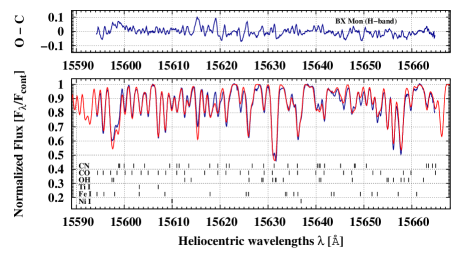
Figure 1: The $H$-band spectrum of BX Mon observed 2003 February (blue line) and a synthetic spectrum (red line) calculated using the final abundances and ¹²C/¹³C isotopic ratio (Table 4).

Figure 2: $H$-band spectra of Hen 3-1213 observed 2003 February (blue line), 2010 May (green line), and a synthetic spectrum (red line) calculated using the final abundances (Table 4).

Figure 3: The $H_{\rm b}$-band spectrum of V694 Mon observed 2010 March (blue line) and a synthetic spectrum (red line) calculated using the final abundances and ¹²C/¹³C isotopic ratio (Table 4).

Figure 4: $K$-band spectra of Hen 3-1761 observed 2003 August (blue line), 2004 April (green line), and a synthetic spectrum (red line) calculated using the final abundances (Table 4).

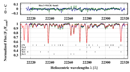
Figure 5: $K$-band spectra of Hen 3-916 observed 2003 April (blue line), 2004 April (green line), and a synthetic spectrum (red line) calculated using the final abundances (Table 4).

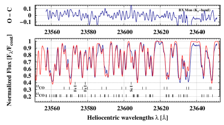
Figure 6: The $K_{\rm r}$-band spectrum of BX Mon observed 2006 April (blue line) and a synthetic spectrum (red line) calculated using the final abundances and ¹²C/¹³C isotopic ratio (Table 4).

Figure 7: The $K_{\rm r}$-band spectrum of RW Hya observed 2006 April (blue line) and a synthetic spectrum (red line) calculated using the final abundances and ¹²C/¹³C isotopic ratio (Table 4).

3 Methods

The analysis technique we employ is the literature standard, i.e. local thermal equilibrium (LTE) analysis based on a 1D, hydrostatic model atmosphere of the star. Despite its shortcomings this remains the most frequently used technique in chemical composition determination. It is known that this approach does not fully reflect reality. The atmospheres of cool giants/supergiants are complex, dynamic, and subject to stratification. A non-LTE (NLTE) approach combined with a 3D treatment of the atmosphere would be a more appropriate model but remains computationally impractical.

Errors introduced by the LTE 1D approach can be qualitatively estimated. There are a very few studies of abundances in stars, especially giants and supergiants, that use NLTE. The technique has been restricted mainly to objects with very low metallicity were NLTE effects are the most significant. Our targets have at most near-solar or barely subsolar metallicities where NLTE effects are relatively weak. It is possible to estimate the magnitude of such corrections. Mashonkina (2014) has calculated NLTE–LTE differences for iron lines through a wide ranges of metallicities and $\log{g}$. While these results do not cover the parameters of our program stars we can nonetheless extrapolate the corrections needed for the target with largest $\log{g}$ and smallest metallicity in our sample. This correction would be of order hundredths of dex. To our knowledge, the only similar studies for near-solar metallicities and low surface gravities characteristic for our giants are those for Si i (Bergemann et al., 2013) and Mg i (Bergemann et al., 2015), implying corrections in the range from approximately $-0.1$ to $-0.4$ in the case of our cool giants with lowest $\log{g}$. Although significant progress in the analysis of stellar spectra with 3D and NLTE models has been made since Asplund (2005) described this field a decade ago, the corrections discussed in detail by Bergemann (2014) are available for single lines only, and they do not correspond to the stellar parameters and the wavelength ranges used in our work.

To determine chemical abundances we used LTE spectral synthesis techniques particularly suited for strongly blended spectra. Our spectra are heavily blended. For instance, only in the $K$-band region can atomic lines be found that are significantly stronger than the background of weak molecular CN lines. With the exception of these lines the reliable measurement of equivalent widths of individual lines is practically impossible. The synthetic spectra in our study were calculated with use of WIDMO code (Schmidt et al., 2006). 1D hydrostatic MARCS model atmospheres by Gustafsson et al. (2008) were employed. In selected cases our results were verified with use of TURBOSPECTRUM spectral synthesis code (Alvarez & Plez 1998; Plez 2012). TURBOSPECTRUM and WIDMO produced almost identical synthetic spectra. The method of fitting the synthetic spectra to the observations is similar to that described earlier in Papers I and II. Some small changes were implemented and are described below.

The line lists, with the excitation potentials and $gf$-values for transitions, for the atomic and molecular lines are largely the same as in our previous analyses (Papers I and II). For $K$- and $K_{\rm r}$-band regions the atomic data are from the Vienna Atomic Line Database (VALD) (Kupka et al., 1999). For the $H$- and $H_{\rm b}$-band regions the list by Mélendez & Barbuy (1999) was used. For the molecular data we used the lists of Goorvitch (1994) for CO and of Kurucz (1999) for OH. In the case of CN the Kurucz compilation that we previously used was replaced with the recent line list by Sneden et al. (2014). The use of the Sneden et al. (2014) list greatly improved the fitting of the CN spectrum.

To perform the spectral synthesis the stellar parameters, effective temperature $T_{\rm{eff}}$, surface gravity $\log{g}$, and the atmospheric motion turbulence parameters, the micro ($\xi_{\rm t}$) and macro ($\zeta_{\rm t}$) turbulence velocities, must be specified and introduced as inputs into the calculations. To obtain $T_{\rm{eff}}$ and $\log{g}$ the method traditionally employed uses neutral and ionized lines of the same species, usually of iron. Under the approximation of ionization equilibria the abundances obtained from the two sets of lines should not depend on the ionization stage or the excitation energy (eg. Plez, 2013). Similarly the microturbulent velocities ($\xi_{\rm t}$) are commonly determined by requiring that abundances resulting from individual lines of the same species, but with differing line strengths, be independent of equivalent width (e.g. Smith et al. 2002; Schmidt et al. 2006).

However, our spectra do not have lines present from ionized elements. Similarly, we do not have a sample of unblended lines with different intensities for the same elements. The estimation of effective temperature $T_{\rm{eff}}$ was based, instead, on spectral types (Table 2). The spectral types we employ were derived by Mürset & Schmid (1999) from TiO bands in the near-IR. The accuracy of the temperature classification is approximately one spectral subclass. The only object in our sample, SS73 96, for which Mürset & Schmid (1999) have not performed spectral classification was assigned spectral type M0 and M2 by Medina Tanco & Steiner (1970) and Allen (1980), respectively. Our $K$-band spectrum casts doubt on these classifications. The CN lines resemble those in the spectra for the other cool stars. The hottest stars in our sample, RW Hya and Hen 3-1213, have much weaker CN lines. Re-analysing the strength of TiO bands heads in the $\sim$7000–9500 Å spectral region and the calcium triplet Ca ii in the spectrum published by Medina Tanco & Steiner (1970) we find that M5 is a more suitable classification for this giant. The calibrations of Richichi et al. (1999) and Van Belle et al. (1999) were used to translate the spectral types into effective temperatures. The effective temperatures are listed in Table 2. The uncertainty in these temperatures are estimated as $\sim$100 K.

Table 2: Estimates of the stellar effective temperature $T_{\rm{eff}}$ and surface gravity $\log{g}$ using the techniques and calibrations indicated.

	Sp. type[1]	$T_{\rm{eff}}^{[2]}$	$T_{\rm{eff}}^{[3]}$	$J-K^{[4,5]}$	$E$($B-V$)[6]	($J-K$)0	$T_{\rm{eff}}^{[7]}$	$\log{g}$[7]	$\log{g}$[8]	$T_{\rm{eff}}^{a}$	$\log{g}^{a}$
		(K)	(K)	(mag)	(mag)	(mag)	(K)			[K]
BX Mon	M5	3355 $\pm$ 75	3367	1.37$\pm$0.06	$<$0.14$\pm$0.02	$>$1.30$\pm$0.07	$<$3250$\pm$150	$<$0.0$\pm$0.2	0.3–0.6	3400	0.0
V694 Mon	M6	3240 $\pm$ 75	3258	1.42$\pm$0.07	$<$0.22$\pm$0.01	$>$1.32$\pm$0.08	$<$3210$\pm$170	$<-0.1\pm$0.3	0.1–0.4	3300	0.0
Hen 3-461	M7	3100 $\pm$ 80	3149	1.41$\pm$0.32	$<$0.42$\pm$0.02	$>$1.21$\pm$0.34	$\sim$3440	$\sim$0.3	0.0–0.3	3200	0.0
SY Mus	M5	3355 $\pm$ 75	3367	1.37$\pm$0.07	0.4–0.5	$\sim$1.20	$<$3500	$<$0.39	0.3–0.6	3400	0.5
Hen 2-87	M5.5	3300 $\pm$ 75	3312	2.60$\pm$0.08	$<\sim$6.1	–	–	–	0.2–0.5	3300	0.5
Hen 3-828	M6	3240 $\pm$ 75	3258	1.48$\pm$0.07	$<$0.37$\pm$0.02	$>$1.30$\pm$0.09	$<$3250$\pm$190	$<$0.0$\pm$0.3	0.1–0.4	3300	0.0
CD-36∘8436	M5.5	3300 $\pm$ 75	3312	1.27$\pm$0.06	$<$0.05$\pm$0.01	$>$1.25$\pm$0.07	$<$3360$\pm$70	$<$0.1$\pm$0.1	0.2–0.5	3300	0.0
RW Hya	M2	3655 $\pm$ 80	3695	1.12$\pm$0.07	$<$0.07$\pm$0.01	$>$1.09$\pm$0.07	$<$3690$\pm$150	$<$0.7$\pm$0.2	0.8–1.1	3700	0.5
Hen 3-916	M5	3355 $\pm$ 75	3367	1.63$\pm$0.08	$<$1.25$\pm$0.05	$>$1.02$\pm$0.13	$<$3850±280	$<$1.0$\pm$0.5	0.3–0.6	3400	0.5
Hen 3-1092	M5.5	3300 $\pm$ 75	3312	1.29$\pm$0.06	$<$0.11$\pm$0.01	$>$1.24$\pm$0.07	$<$3380$\pm$140	$<$0.2$\pm$0.2	0.2–0.5	3300	0.0
WRAY 16-202	M6	3240 $\pm$ 75	3258	2.09$\pm$0.06	$<\sim$3.1	–	–	–	0.1–0.4	3300	0.0
Hen 3-1213	$\leq$K4	$\leq$4080 $\pm$ 120	$\leq$4132	1.37$\pm$0.08	$<$1.07$\pm$0.03	$>$0.85$\pm$0.12	$<$4240$\pm$285	$<$1.8$\pm$0.6	–	4100	1.5
Hen 2-173	M4.5	3410 $\pm$ 75	3421	1.68$\pm$0.07	$<$0.67$\pm$0.06	$>$1.35$\pm$0.14	$<$3150$\pm$290	$<-0.2\pm$0.5	0.3–0.6	3400	0.5
KX Tra	M6	3240 $\pm$ 75	3258	1.39$\pm$0.07	$<$0.17$\pm$0.01	$>$1.30$\pm$0.06	$<$3250$\pm$120	$<$0.0$\pm$0.2	0.1–0.4	3300	0.0
CL Sco	M5	3355 $\pm$ 75	3367	1.29$\pm$0.06	$<$0.28$\pm$0.01	$>$1.15$\pm$0.07	$<$3570$\pm$150	$<$0.5$\pm$0.3	0.3–0.6	3400	0.5
V455 Sco	M6.5	3170 $\pm$ 80	3203	1.62$\pm$0.07	$<$0.67$\pm$0.03	$>$1.29$\pm$0.10	$<$3270$\pm$210	$<$0.0$\pm$0.4	0.0–0.3	3200	0.0
Hen 2-247	M6	3240 $\pm$ 75	3258	1.61$\pm$0.07	$<$0.60$\pm$0.01	$>$1.31$\pm$0.08	$<$3230$\pm$160	$<-0.1\pm$0.3	0.1–0.4	3300	0.0
RT Ser	M6	3240 $\pm$ 75	3258	1.56$\pm$0.07	$<$0.48$\pm$0.01	$>$1.32$\pm$0.08	$<$3210$\pm$150	$<-0.1\pm$0.3	0.1–0.4	3300	0.0
AE Ara	M5.5	3300 $\pm$ 75	3312	1.36$\pm$0.06	$<$0.20$\pm$0.01	$>$1.26$\pm$0.06	$<$3330$\pm$150	$<$0.1$\pm$0.2	0.2–0.5	3300	0.5
SS73 96	M5b	3355 $\pm$ 75	3367	1.81$\pm$0.07	$<$1.23$\pm$0.03	$>$1.21$\pm$0.10	$<$3430$\pm$210	$<$0.3$\pm$0.4	0.3–0.6	3400	0.5
AS 270	M5.5	3300 $\pm$ 75	3312	1.75$\pm$0.07	$<\sim$7.3	–	–	–	0.2–0.5	3300	0.5
Y CrA	M6	3240 $\pm$ 75	3258	1.33$\pm$0.06	$<$0.12$\pm$0.01	$>$1.27$\pm$0.07	$<$3300$\pm$140	$<$0.0$\pm$0.2	0.1–0.4	3300	0.0
Hen 2-374	M5.5	3300 $\pm$ 75	3312	2.06$\pm$0.08	$<$1.74$\pm$0.11	$>$1.21$\pm$0.21	$<$3440$\pm$450	$<$0.3$\pm$0.8	0.2–0.5	3300	0.5
Hen 3-1761	M5.5	3300 $\pm$ 75	3312	1.27$\pm$0.06	$<$0.08$\pm$0.01	$>$1.23$\pm$0.06	$<$3390$\pm$130	$<$0.2$\pm$0.2	0.2–0.5	3300	0.0

• spectral types from ^[1]Mürset & Schmid (1999), total Galactic extinction adopted according to ^[6]Schlafly & Finkbeiner (2011) and Schlegel, Finkbeiner & Davis (1998), infrared colours from 2MASS ^[4](Phillips, 2007) transformed to ^[5]Bessell & Brett (1988) photometric system.

• ^[2]Richichi et al. (1999), ^[3]Van Belle et al. (1999), ^[7]Kucinskas et al. (2005), ^[8]Dumm & Schild (1998) for the red giant masses in the range 1–2M_☉.

• type M5 adopted – see the text for explanation.

All our targets have Two Micron All Sky Survey (2MASS) $J$ and $K$ magnitudes (Phillips, 2007). Combining the 2MASS colours with colour excesses (Schlegel, Finkbeiner & Davis 1998; Schlafly & Finkbeiner 2011) provides an estimate of the IR intrinsic colours. Upper limits to the effective temperature and surface gravity were then derived according to the Kucinskas et al. (2005) $T_{\rm{eff}}$–$\log{g}$–colour relation for late-type giants. The effective temperatures derived from spectral type calibrations fall below these limits. Independent estimates for $\log{g}$ have also been obtained (Table 2) by assuming that the masses of symbiotic giants are in the range $\sim$1–2 M_☉ (Mikołajewska, 2003) and that their radii follow the radius–spectral type relation from Dumm & Schild (1998, table 2). In some cases we can also place additional constraints on $\log{g}$ from the orbital solution of the red giant in the symbiotic binary (Table 3). A limit can be set on the giant radius using the inclination. The mass can be estimated from the most probable orbital solutions.

The $T_{\rm{eff}}$ and $\log{g}$ adopted for the atmosphere models used in our calculations are shown in the rightmost columns of Table 2. The uncertainty in the $\log{g}$ is difficult to estimate. However, the limitations on this parameter obtained with the various methods discussed above give consistent results. The uncertainty in the adopted values should not be larger than $\sim 0.5$ which is the resolution of the MARCS model atmosphere grid used in our calculations.

In our previous studies (Papers I and II), as well as in the initial phase of the current work, we tried holding the microturbulent velocity, $\xi_{\rm{t}}$, as a free parameter. We searched for its value by sampling in the range 1.2–2.8 km s^-1. We obtained microturbulences close to 2 km s^-1 with a dispersion $\sim\pm$0.35. $\xi_{\rm{t}}=2.0$ km s^-1 is typical for cool Galactic red giants (Smith & Lambert 1985, 1986, 1990) and is frequently used in studies of chemical compositions (e.g. Neyskens et al., 2015). We subsequently decided to use $\xi_{\rm{t}}=2.0$ km s^-1 as the input to our models. Similarly the macroturbulent velocity was set to the typical value for cool red giants $\zeta_{\rm{t}}$ = 3 km s^-1 (e.g. Fekel, Hinkle & Joyce, 2003).

Table 3: Estimates of surface gravities employing most probable mass and radius from orbital solutions.

Object	$M_{\rm{rg}}[$M${}_{\sun}]$	$R_{\rm{rg}}[$R${}_{\sun}]$	$\log{g}$	Ref.a
BX Mon	$1.5^{b}$	$160\pm 50$	$+0.5$– $0.0$	$[1]$
SY Mus	$1.3\pm 0.25$	$135$	$+0.4$–$+0.2$	$[2]$
CD-36∘8436	$1.5$	$112$–$192$	$+0.5$– $0.0$	$[7]$
RW Hya	$3.4$	$145$	$+0.6$	$[3]$
Hen 3-1213	$1.0$	$53$–$107$	$+1.0$–$+0.4$	$[7]$
Hen 2-173	$1.5$	$100$–$149$	$+0.6$–$+0.3$	$[4]$
CL Sco	$1.5$	$75$–$114$	$+0.9$–$+0.5$	$[4]$
V455 Sco	$1.12$	$207\pm 28$	$0.0$–$-0.3$	$[5]$
Hen 2-247	$1.2$	$137\pm 15$	$+0.3$–$+0.1$	$[5]$
AE Ara	$1.6$	$111$–$166$	$+0.6$–$+0.2$	$[6]$
SS73 96	$1.5$	$94\pm 12$	$+0.8$–$+0.6$	$[7]$
AS 270	$1.5$	$119$–$171$	$+0.5$–$+0.1$	$[4]$
Hen 2-374	$1.6$	$114$–$131$	$+0.5$–$+0.4$	$[6]$

• for masses and radii adopted for $\log{g}$ estimations: $[1]$ Dumm et al. (1998); $[2]$ Rutkowski et al. (2007); $[3]$ Otulakowska-Hypka et al. (2014); $[4]$ Fekel et al. (2007); $[5]$ Fekel et al. (2008); $[6]$ Fekel et al. (2010); $[7]$ Fekel et al. (2015).

• mass adopted according to Brandi et al. (2009) (see Paper II for the details).

The observed spectra are also affected by large-scale motions, e.g. radial and rotational velocities as well as velocity shifts introduced by the instrument, e.g. flexure. These all have to be taken into account to enable calculations of residuals (’observations minus model’) in order to perform the minimization. The wavelength shifts originating from combination of radial velocities and instrumental effects were determined with the IRAF cross-correlation program FXCOR (Fitzpatrick, 1993). The synthetic spectrum was used for the templates. The observed spectra were wavelength shifted to match the position of the spectral lines in synthetic spectra.

In our sample the largest contribution to the broadening of the spectral lines is the giant star rotational velocity, $V_{\rm{rot}}\sin{i}$. To measure $V_{\rm{rot}}\sin{i}$ we used two methods: (i) a cross-correlation technique CCF similar to that adopted by Carlberg et al. (2011) but using synthetic spectra as the templates and (ii) direct measurement of the FWHM of the six relatively strong unblended atomic lines (Ti i, Fe i, Sc i) present in the $K$-band region. The measured values are presented in Table 1. The rotational velocities obtained with CCF method are generally somewhat smaller than those obtained with FWHM method. Spectral regions that are crowded with blended molecular lines, as found in the $H$-band spectra, lead to an underestimate. We compared $V_{\rm{rot}}\sin{i}$ obtained with both these methods (CCF and FWHM) when the rotational velocities were allowed to be free parameters in the solution process (Paper I). The differences were not significant with the changes in $V_{\rm{rot}}\sin{i}$ having small impact in the resulting abundances. Our analysis uses $V_{\rm{rot}}\sin{i}$ obtained from atomic lines in $K$-band spectra with the FWHM method and applied to all of spectra for a given object (Table 1). This value of $V_{\rm{rot}}\sin{i}$ was treated as a fixed parameter in our solution.

The method described in Papers I and II was adopted for the abundance calculations with the difference, discussed above, that the microturbulence was fixed at $\xi_{\rm{t}}$=2 km s^-1. The solutions were performed in a semi-automatic way to improve the efficiency of the $\chi^{2}$ minimization and simultaneously too keep control of the parameter values that were entered. The simplex algorithm (Brandt, 1998) was applied to the parameter space $\chi^{2}$ minimization. The simplex algorithm is a relatively slow least squares technique but it has notable advantages. It is known to be remarkably efficient in achieving convergence when more than two or three parameters need to be adjusted. In our case $n+1=8$, where ’n’ is the number of free parameters. Calculations starting from this number of places in parameter space are efficiently searched for the minimum.

A brief outline of the analysis procedure follows. Initial values for the abundances of oxygen, carbon, and nitrogen were adjusted fitting by eye alternately using OH, CO, and CN lines. Next the abundances of elements around the iron peak were adjusted using atomic lines. This process was repeated iteratively to find approximate parameters of the chemical composition, around which the initial grid of the $n+1$, $n$ dimensional sets of free parameters, the so-called simplex needed for the simplex algorithm, was prepared. Nine different randomly generated simplexes were used to obtain best fits to $H$-, $H_{\rm b}$, and $K$-band spectra and the standard deviations. In the case of the 10 systems where the $K_{\rm r}$-band spectrum had been observed, after we found the sets of parameters that give the best fit to the $H$-, $H_{\rm b}$, and $K$-band spectra, the abundances were then applied to the $K_{\rm r}$-band spectrum as fixed values and a search for ¹²C$/^{13}$C isotopic ratio was performed. Reconciliation of carbon abundance and ¹²C$/^{13}$C required several iterations. Most frequently the $K_{\rm r}$-band region was not observed and an isotopic ratio of ¹²C$/^{13}$C=10 was used in calculations. ¹²C$/^{13}$C=10 is a value close to the average, and median simultaneously, among those stars for which we could obtain isotopic ratios. The above procedure was iteratively repeated, when needed, to choose the model atmosphere with the best-matching metallicity.

4 Results

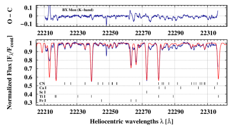
Figure 18: The $K$-band spectrum of BX Mon observed 2003 April (blue line) and a synthetic spectrum (red line) calculated using the final abundances and ¹²C/¹³C isotopic ratio (Table 4).

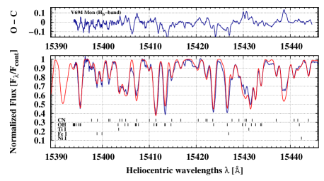
Figure 20: The $H_{\rm b}$-band spectrum of V694 Mon observed 2010 March (blue line) and a synthetic spectrum (red line) calculated using the final abundances and ¹²C/¹³C isotopic ratio (Table 4).

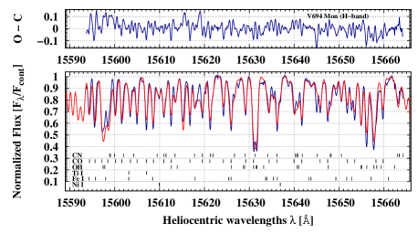
Figure 21: The $H$-band spectrum of V694 Mon observed 2003 February (blue line) and a synthetic spectrum (red line) calculated using the final abundances and ¹²C/¹³C isotopic ratio (Table 4).

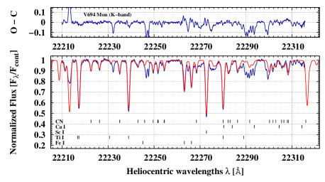
Figure 22: The $K$-band spectrum of V694 Mon observed 2003 April (blue line) and a synthetic spectrum (red line) calculated using the final abundances and ¹²C/¹³C isotopic ratio (Table 4).

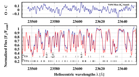
Figure 23: The $K_{\rm r}$-band spectrum of V694 Mon observed 2006 April (blue line) and a synthetic spectrum (red line) calculated using the final abundances and ¹²C/¹³C isotopic ratio (Table 4).

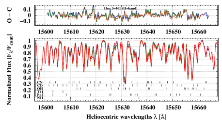
Figure 24: $H$-band spectra of Hen 3-461 observed 2003 February (blue line), 2009 April (green line), 2010 May (dark-orange line), and a synthetic spectrum (red line) calculated using the final abundances and ¹²C/¹³C isotopic ratio (Table 4).

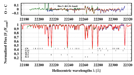
Figure 25: $K$-band spectra of Hen 3-461 observed 2003 April (blue line), 2003 December (green line), 2004 April (dark-orange line), and a synthetic spectrum (red line) calculated using the final abundances (Table 4).

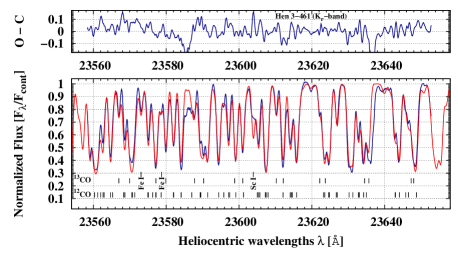
Figure 26: The $K_{\rm r}$-band spectrum of Hen 3-461 observed 2006 April (blue line) and a synthetic spectrum (red line) calculated using the final abundances and ¹²C/¹³C isotopic ratio (Table 4).

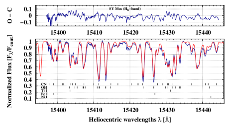
Figure 27: The $H_{\rm b}$-band spectrum of SY Mus observed 2010 March (blue line) and a synthetic spectrum (red line) calculated using the final abundances and ¹²C/¹³C isotopic ratio (Table 4).

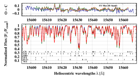
Figure 28: $H$-band spectra of SY Mus observed 2003 February (blue line), 2009 April (green line), 2010 April (dark-orange line), and a synthetic spectrum (red line) calculated using the final abundances and ¹²C/¹³C isotopic ratio (Table 4).

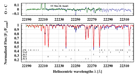
Figure 29: $K$-band spectra of SY Mus observed 2003 April (blue line), 2003 December (green line), and a synthetic spectrum (red line) calculated using the final abundances (Table 4).

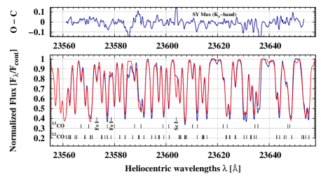
Figure 30: The $K_{\rm r}$-band spectrum of SY Mus observed 2006 April (blue line) and a synthetic spectrum (red line) calculated using the final abundances and ¹²C/¹³C isotopic ratio (Table 4).

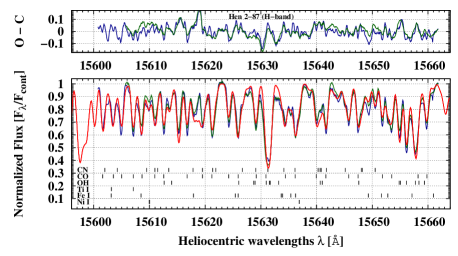
Figure 31: $H$-band spectra of Hen 2-87 observed 2003 February (blue line), 2010 April (green line), and a synthetic spectrum (red line) calculated using the final abundances and ¹²C/¹³C isotopic ratio (Table 4).

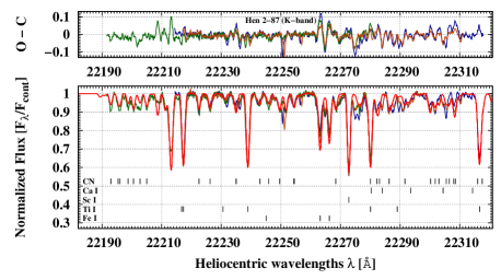
Figure 32: $K$-band spectra of Hen 2-87 observed 2003 April (blue line), 2003 December (green line), 2004 April (dark-orange line), and a synthetic spectrum (red line) calculated using the final abundances (Table 4).

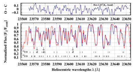
Figure 33: The $K_{\rm r}$-band spectrum of Hen 2-87 observed 2006 April (blue line) and a synthetic spectrum (red line) calculated using the final abundances and ¹²C/¹³C isotopic ratio (Table 4).

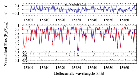
Figure 34: The $H$-band spectrum of Hen 3-828 observed 2003 February (blue line) and a synthetic spectrum (red line) calculated using the final abundances and ¹²C/¹³C isotopic ratio (Table 4).

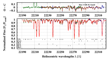
Figure 35: $K$-band spectra of Hen 3-828 observed 2003 April (blue line), 2003 December (green line), 2004 April (dark-orange line), and a synthetic spectrum (red line) calculated using the final abundances (Table 4).

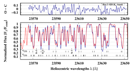
Figure 36: The $K_{\rm r}$-band spectrum of Hen 3-828 observed 2006 April (blue line) and a synthetic spectrum (red line) calculated using the final abundances and ¹²C/¹³C isotopic ratio (Table 4).

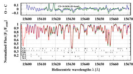
Figure 37: $H$-band spectra of CD-36^∘8436 observed 2003 February (blue line), 2010 April (green line), and a synthetic spectrum (red line) calculated using the final abundances and ¹²C/¹³C isotopic ratio (Table 4).

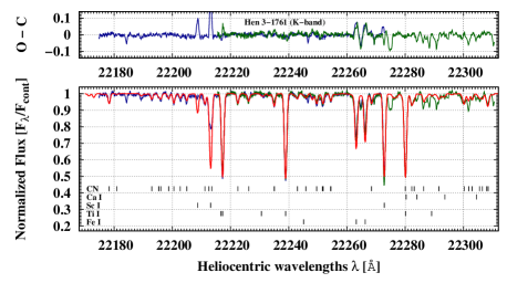
Figure 75: $K$-band spectra of Hen 3-1761 observed 2003 August (blue line), 2004 April (green line), and a synthetic spectrum (red line) calculated using the final abundances (Table 4).

The abundances derived from CNO molecules and atomic lines (Sc i, Ti i, Fe i, Ni i), on the scale of $\log{\epsilon}(X)=\log{(N(X)N(H)^{-1})}+12.0$, are summarized in Table 4 together with the ¹²C/¹³C isotopic ratio, projected rotational velocities ($V_{\rm{rot}}\sin{i}$), and corresponding uncertainties. Synthetic fits to the observed spectra of BX Mon and Hen 3-1213 in $H$-band region, V694 Mon in $H_{\rm b}$-band, Hen 3-1761 and Hen 3-916 in $K$-band, and BX Mon and RW Hya in $K_{\rm r}$-band are shown in Figs 1-7. The molecular (OH, CO, CN) and atomic (Sc i, Ti i, Fe i, Ni i) lines used in solving of the chemical composition are identified. The synthetic fits to all the observed spectra are shown in Figs 17-75 in the online Appendix B. Systematic effects are possible due to the choice of model atmospheres. We made a comparison of abundances obtained with the PHOENIX model atmospheres extracted from Hauschildt et al. (1999) used for five selected cases of BX Mon, Hen 3-461, SY Mus, Hen 2-173, and CL Sco. The use of PHOENIX models lead to somewhat higher abundances by on average $\sim$0.1, $\sim$0.16, $\sim$0.22, $\sim$0.13, $\sim$0.1, $\sim$0.01, and $\sim$0.02 dex for C, N, O, Sc, Ti, Fe, and Ni, respectively.

The atmospheric parameters have associated uncertainties of $\sim$100 K in effective temperature, up to 0.5 in $\log{g}$, and $\sim$0.25 km s^-1 in the case of microturbulence. The latter is the largest uncertainty which we previously obtained when microturbulence was considered as the free parameter. To investigate how these uncertainties manifest themselves as abundance changes, we made additional fits with MARCS atmosphere models varying the atmospheric parameters by the values of the uncertainties ($\Delta T_{\mathrm{eff}}=\pm$100 K, $\Delta\log{g}=\pm$0.5, $\Delta\xi_{\mathrm{t}}=\pm$0.25). The changes in the abundance obtained for each element as a function of each model parameter are listed in Table 5 at the top for M giants and separately at the bottom for the yellow symbiotic Hen 3-1213. In the case of Hen 3-1213 the dependences on the uncertainties in stellar parameters are significantly different than for the M giants. The final estimated uncertainty for each element is the quadrature sum of each model uncertainty. It is shown in the rightmost column of Table 5, marked with $\Delta$ symbol. By comparing Tables 4 and 5 we can see that the uncertainties of the derived chemical composition come mainly from uncertainties in the atmospheric parameters. With a few exceptions, the uncertainties associated with the fitting, originating mainly from line-to-line dispersion due to line blending, continuum problems, uncertainties on oscillator strengths, etc. are less important. The uncertainty in $\log{g}$ can have large impact on the carbon abundances and, in the case of cool M-type giants, the uncertainty in the adopted microturbulence can have a large impact on the abundances of scandium and titanium.

Table 4: Calculated and relative abundances, rotational velocity, and uncertainties$\,{}^{a}$ derived for 24 S-type symbiotic systems.

	C	N	O	Scb	Ti	Fe	Ni	12C/13C	$V_{\mathrm{rot}}\sin{i}$
	$\log{\epsilon(X)}$								$(\mathrm{km}\,\mathrm{s}^{-1})$
	[$X$]c
BX Mon	7.69$\pm$0.02	7.79$\pm$0.05	8.20$\pm$0.01	3.59$\pm$0.13	4.71$\pm$0.05	7.07$\pm$0.04	6.05$\pm$0.11	8$\pm$1	8.4$\pm$1.4
	-0.74$\pm$0.07	-0.04$\pm$0.10	-0.49$\pm$0.06	+0.43$\pm$0.17	-0.22$\pm$0.10	-0.40$\pm$0.08	-0.15$\pm$0.15
V694 Mon	8.08$\pm$0.01	7.90$\pm$0.02	8.40$\pm$0.01	4.01$\pm$0.07	4.54$\pm$0.05	7.12$\pm$0.04	5.86$\pm$0.06	23$\pm$2	8.2$\pm$1.0
	-0.35$\pm$0.06	+0.07$\pm$0.07	-0.29$\pm$0.06	+0.85$\pm$0.11	-0.39$\pm$0.10	-0.35$\pm$0.08	-0.34$\pm$0.10
Hen 3-461	8.29$\pm$0.02	8.35$\pm$0.04	8.74$\pm$0.01	4.14$\pm$0.06	5.16$\pm$0.06	7.59$\pm$0.07	6.48$\pm$0.05	13$\pm$1	7.4$\pm$0.6
	-0.14$\pm$0.07	+0.52$\pm$0.09	+0.05$\pm$0.06	+0.98$\pm$0.10	+0.23$\pm$0.11	+0.12$\pm$0.11	+0.28$\pm$0.09
SY Mus	8.07$\pm$0.02	8.12$\pm$0.04	8.61$\pm$0.02	3.96$\pm$0.12	4.93$\pm$0.04	7.32$\pm$0.04	6.13$\pm$0.09	8$\pm$2	6.6$\pm$0.6
	-0.36$\pm$0.07	+0.29$\pm$0.09	-0.08$\pm$0.07	+0.80$\pm$0.16	0.00$\pm$0.09	-0.15$\pm$0.08	-0.07$\pm$0.13
Hen 2-87	8.61$\pm$0.02	8.30$\pm$0.05	8.99$\pm$0.02	3.93$\pm$0.10	4.74$\pm$0.04	7.64$\pm$0.05	6.41$\pm$0.07	18$\pm$2	9.6$\pm$0.6
	+0.18$\pm$0.07	+0.47$\pm$0.10	+0.30$\pm$0.07	+0.77$\pm$0.14	-0.19$\pm$0.09	+0.17$\pm$0.09	+0.21$\pm$0.11
Hen 3-828	8.30$\pm$0.03	8.21$\pm$0.04	8.71$\pm$0.01	4.61$\pm$0.06	5.43$\pm$0.07	7.50$\pm$0.05	6.17$\pm$0.07	15$\pm$2	7.9$\pm$0.5
	-0.13$\pm$0.08	+0.38$\pm$0.09	+0.02$\pm$0.06	+1.45$\pm$0.10	+0.50$\pm$0.12	+0.03$\pm$0.09	-0.03$\pm$0.11
CD-36∘8436	7.74$\pm$0.01	7.99$\pm$0.03	8.36$\pm$0.01	3.66$\pm$0.07	4.71$\pm$0.06	7.17$\pm$0.03	6.00$\pm$0.09	8$\pm$1	8.1$\pm$1.1
	-0.69$\pm$0.06	+0.16$\pm$0.08	-0.33$\pm$0.06	+0.50$\pm$0.11	-0.22$\pm$0.11	-0.30$\pm$0.07	-0.20$\pm$0.13
RW Hya	7.52$\pm$0.04	7.48$\pm$0.08	8.14$\pm$0.03	2.65$\pm$0.09	4.35$\pm$0.06	6.70$\pm$0.04	5.67$\pm$0.05	5.3$\pm$0.5	6.2$\pm$0.9
	-0.91$\pm$0.09	-0.35$\pm$0.13	-0.55$\pm$0.08	-0.51$\pm$0.13	-0.58$\pm$0.11	-0.77$\pm$0.08	-0.53$\pm$0.09
Hen 3-916	7.99$\pm$0.02	7.90$\pm$0.05	8.30$\pm$0.01	3.39$\pm$0.09	4.67$\pm$0.07	7.01$\pm$0.04	5.77$\pm$0.07	6.6$\pm$0.6	8.5$\pm$0.9
	-0.44$\pm$0.07	+0.07$\pm$0.10	-0.39$\pm$0.06	+0.23$\pm$0.13	-0.26$\pm$0.12	-0.46$\pm$0.08	-0.43$\pm$0.11
Hen 3-1092	7.41$\pm$0.02	7.47$\pm$0.03	8.04$\pm$0.02	3.33$\pm$0.18	4.21$\pm$0.08	6.68$\pm$0.07	5.57$\pm$0.13	–	5.8$\pm$0.7
	-1.02$\pm$0.07	-0.36$\pm$0.08	-0.65$\pm$0.07	+0.17$\pm$0.22	-0.72$\pm$0.13	-0.79$\pm$0.11	-0.63$\pm$0.17
WRAY 16-202	8.11$\pm$0.02	8.24$\pm$0.05	8.66$\pm$0.01	4.37$\pm$0.18	5.37$\pm$0.13	7.64$\pm$0.05	6.37$\pm$0.06	10$\pm$1	8.3$\pm$1.7
	-0.32$\pm$0.07	+0.41$\pm$0.10	-0.03$\pm$0.06	+1.21$\pm$0.22	+0.44$\pm$0.18	+0.17$\pm$0.09	+0.17$\pm$0.10
Hen 3-1213	8.00$\pm$0.03	7.76$\pm$0.04	8.88$\pm$0.02	3.29$\pm$0.09	4.98$\pm$0.06	6.79$\pm$0.04	5.70$\pm$0.11	–	7.4$\pm$0.3
	-0.43$\pm$0.08	-0.07$\pm$0.09	+0.19$\pm$0.07	+0.13$\pm$0.13	+0.05$\pm$0.11	-0.68$\pm$0.08	-0.50$\pm$0.15
Hen 2-173	8.18$\pm$0.03	8.17$\pm$0.07	8.80$\pm$0.02	3.94$\pm$0.11	5.12$\pm$0.09	7.29$\pm$0.04	6.16$\pm$0.06	–	8.4$\pm$0.6
	-0.25$\pm$0.08	+0.34$\pm$0.12	+0.11$\pm$0.07	+0.78$\pm$0.15	+0.19$\pm$0.14	-0.18$\pm$0.08	-0.04$\pm$0.10
KX TrA	8.02$\pm$0.03	7.90$\pm$0.09	8.62$\pm$0.03	3.87$\pm$0.12	4.99$\pm$0.15	7.13$\pm$0.07	6.09$\pm$0.11	–	8.5$\pm$1.3
	-0.41$\pm$0.08	+0.07$\pm$0.14	-0.07$\pm$0.08	+0.71$\pm$0.16	+0.06$\pm$0.20	-0.34$\pm$0.11	-0.11$\pm$0.15
CL Sco	7.98$\pm$0.04	8.19$\pm$0.09	8.57$\pm$0.02	3.39$\pm$0.13	4.79$\pm$0.10	7.16$\pm$0.03	6.15$\pm$0.13	–	7.8$\pm$0.8
	-0.45$\pm$0.09	+0.36$\pm$0.14	-0.12$\pm$0.07	+0.23$\pm$0.17	-0.14$\pm$0.15	-0.31$\pm$0.07	-0.05$\pm$0.17
V455 Sco	8.42$\pm$0.02	8.81$\pm$0.07	9.16$\pm$0.03	4.20$\pm$0.10	5.37$\pm$0.05	7.83$\pm$0.05	6.41$\pm$0.10	–	8.4$\pm$1.0
	-0.01$\pm$0.07	+0.98$\pm$0.12	+0.47$\pm$0.08	+1.04$\pm$0.14	+0.44$\pm$0.10	+0.36$\pm$0.09	+0.21$\pm$0.14
Hen 2-247	8.28$\pm$0.02	8.55$\pm$0.05	8.98$\pm$0.01	4.43$\pm$0.09	5.48$\pm$0.09	7.63$\pm$0.05	6.36$\pm$0.06	–	10.4$\pm$1.0
	-0.15$\pm$0.07	+0.72$\pm$0.10	+0.29$\pm$0.06	+1.27$\pm$0.13	+0.55$\pm$0.14	+0.16$\pm$0.09	+0.16$\pm$0.10
RT Ser	8.01$\pm$0.12	7.93$\pm$0.27	8.36d	3.88$\pm$0.10	4.89$\pm$0.08	6.96$\pm$0.04	5.73d	–	7.8$\pm$1.7
	-0.42$\pm$0.17	+0.10$\pm$0.32	-0.33	+0.72$\pm$0.14	-0.04$\pm$0.13	-0.51$\pm$0.08	-0.47
AE Ara	8.25$\pm$0.02	8.14$\pm$0.06	8.66$\pm$0.02	4.20$\pm$0.10	5.22$\pm$0.07	7.45$\pm$0.05	6.23$\pm$0.09	–	10.1$\pm$0.8
	-0.18$\pm$0.07	+0.31$\pm$0.11	-0.03$\pm$0.07	+1.04$\pm$0.14	+0.29$\pm$0.12	-0.02$\pm$0.09	+0.03$\pm$0.13
SS73 96	8.27$\pm$0.03	7.83$\pm$0.08	8.58$\pm$0.02	3.71$\pm$0.21	4.75$\pm$0.14	7.23$\pm$0.07	5.96$\pm$0.26	–	9.1$\pm$0.4
	-0.16$\pm$0.08	+0.00$\pm$0.13	-0.11$\pm$0.07	+0.55$\pm$0.25	-0.18$\pm$0.19	-0.24$\pm$0.11	-0.24$\pm$0.30
AS 270	8.26$\pm$0.02	8.09$\pm$0.03	8.63$\pm$0.01	3.89$\pm$0.18	4.95$\pm$0.07	7.50$\pm$0.03	6.20$\pm$0.11	–	10.0$\pm$0.9
	-0.17$\pm$0.07	+0.26$\pm$0.08	-0.06$\pm$0.06	+0.73$\pm$0.22	+0.02$\pm$0.12	+0.03$\pm$0.07	0.00$\pm$0.15
Y CrA	7.84$\pm$0.01	7.86$\pm$0.03	8.43$\pm$0.02	3.40$\pm$0.06	4.83$\pm$0.04	7.07$\pm$0.02	5.94$\pm$0.05	–	10.4$\pm$2.9
	-0.59$\pm$0.06	+0.03$\pm$0.08	-0.26$\pm$0.07	+0.24$\pm$0.10	-0.10$\pm$0.09	-0.40$\pm$0.06	-0.26$\pm$0.09
Hen 2-374	7.85$\pm$0.08	7.99$\pm$0.12	8.36d	3.87$\pm$0.04	4.90$\pm$0.03	6.95$\pm$0.04	5.73d	–	6.4$\pm$0.5
	-0.58$\pm$0.13	+0.16$\pm$0.17	-0.33	+0.71$\pm$0.08	-0.03$\pm$0.08	-0.52$\pm$0.08	-0.47
Hen 3-1761	7.81$\pm$0.02	7.79$\pm$0.03	8.30$\pm$0.02	3.63$\pm$0.09	4.77$\pm$0.06	7.22$\pm$0.04	6.17$\pm$0.06	–	6.9$\pm$0.6
	-0.62$\pm$0.07	-0.04$\pm$0.08	-0.39$\pm$0.07	+0.47$\pm$0.13	-0.16$\pm$0.11	-0.25$\pm$0.08	-0.03$\pm$0.10
Sun	8.43$\pm$0.05	7.83$\pm$0.05	8.69$\pm$0.05	3.16$\pm$0.04	4.93$\pm$0.04	7.47$\pm$0.04	6.20$\pm$0.04

• abundance of scandium is based on only one strong Sc i line at $\lambda\sim 22272.8$Å  and it may be less reliable than other abundances. Broadening of the
  infrared scandium lines by hyperfine structure has not been included in the analysis (see Paper I).

• to the Sun [$X$] abundances estimated in relation to the solar composition of Asplund et al. (2009) for CNO and Scott et al. (2015) for elements around the iron peak.

5 Discussion

We measured the photospheric chemical abundances (CNO and elements around the iron peak: Sc, Ti, Fe, and Ni) for the first time in a sample 23 classical S-type symbiotic systems with red giant primary and in one yellow-type symbiotic system Hen 3-1213. The abundances of carbon, nitrogen, oxygen, iron, and titanium are based on the large number of absorption features in the spectra and should be relatively well determined. As shown above, the uncertainties are typically $\sim$0.2–0.3 dex ranging up to $\sim$0.4 dex for the case of titanium. Elemental abundances in symbiotic giants can be used to address number of issues, for example to investigate the evolutionary status of these systems and to associate the systems with their parent populations in the Milky Way. Table 6 summarizes absolute abundances of carbon and nitrogen, and relative abundances $[$O$/$Fe$]$, $[$Ti$/$Fe$]$, and $[$Fe$/$H$]$.

The metal abundances in the yellow symbiotic Hen 3-1213 in our sample were studied previously by Pereira & Roig (2009). They find $\log{\epsilon(\mbox{Fe\,{\sc i}})}$ = 6.59 $\pm$ 0.16, $\log{\epsilon(\mbox{Ni\,{\sc i}})}$ = 5.38 $\pm$ 0.15, and $\log{\epsilon(\mbox{Ti\,{\sc i}})}$ = 4.68 based on analysis of optical spectra. Their values are lower by $\sim$0.2–0.3 dex than ours but consistent within the uncertainties. Taking into account that our adopted $\log{g}=1.5$ is higher than the $\log{g}=1.1$ adopted by Pereira & Roig (2009) and given the sensitivity of Fe, Ni, and Ti abundances to $\log{g}$ (Table 5) the agreement between our results is even better, in the case of iron almost perfect to $\sim$0.1 dex.

Table 5: Sensitivity of abundances to uncertainties in the stellar parameters for M-type giants (top) and the yellow symbiotic Hen 3-1213 (bottom).

$\Delta X$	$\Delta T_{\mathrm{eff}}=+100$ K	$\Delta\log{g}=+0.5$	$\Delta\xi_{\mathrm{t}}=+0.25$	$\Delta^{a}$
M-type giants
C	+0.02	+0.23	-0.05	$\pm$0.23
N	+0.03	+0.02	-0.05	$\pm$0.06
O	+0.12	+0.08	-0.06	$\pm$0.16
Sc	+0.10	+0.15	-0.30	$\pm$0.35
Ti	+0.06	+0.15	-0.24	$\pm$0.29
Fe	-0.05	+0.16	-0.08	$\pm$0.18
Ni	-0.06	+0.18	-0.11	$\pm$0.22
Hen 3-1213
C	+0.05	+0.20	0.00	$\pm$0.21
N	+0.10	-0.05	-0.04	$\pm$0.12
O	+0.20	0.00	-0.04	$\pm$0.20
Sc	+0.18	+0.03	-0.05	$\pm$0.19
Ti	+0.17	+0.06	-0.11	$\pm$0.21
Fe	+0.02	+0.11	-0.06	$\pm$0.13
Ni	-0.01	+0.10	-0.05	$\pm$0.11

• $[(\Delta T_{\mathrm{eff}})^{2}+(\Delta\log{g})^{2}+(\Delta\xi_{\mathrm{t}})^{2}]^{0.5}$.

Table 6: Absolute and relative abundances adopted for comparison with Galactic stellar populations. Abundances of CH Cyg and V2116 Oph from the literature are shown for comparison at the bottom.

Object	$A$(12C)	$A$(14N)	$[$O$/$Fe$]$	$[$Ti$/$Fe$]$	$[$Fe$/$H$]$
BX Mon	7.64	7.79	-0.09	+0.18	-0.40
V694 Mon	8.06	7.90	+0.06	-0.04	-0.35
Hen 3-461	8.26	8.35	-0.07	+0.11	+0.12
SY Mus	8.02	8.12	+0.07	+0.15	-0.15
Hen 2-87	8.59	8.30	+0.13	-0.36	+0.17
Hen 3-828	8.27	8.21	-0.01	+0.47	+0.03
CD-36∘8436	7.69	7.99	-0.03	+0.08	-0.30
RW Hya	7.43	7.48	+0.22	+0.19	-0.77
Hen 3-916	7.92	7.90	+0.07	+0.20	-0.46
Hen 3-1092	7.36	7.47	+0.14	+0.07	-0.79
WRAY 16-202	8.06	8.24	-0.20	+0.27	+0.17
Hen 3-1213	7.95	7.76	+0.87	+0.73	-0.68
Hen 2-173	8.13	8.17	+0.29	+0.37	-0.18
KX TrA	7.97	7.90	+0.27	+0.40	-0.34
CL Sco	7.93	8.19	+0.19	+0.17	-0.31
V455 Sco	8.37	8.81	+0.11	+0.08	+0.36
Hen 2-247	8.23	8.55	+0.13	+0.39	+0.16
RT Ser	7.96	7.93	+0.18	+0.47	-0.51
AE Ara	8.20	8.14	-0.01	+0.31	-0.02
SS73 96	8.22	7.83	+0.13	+0.06	-0.24
AS 270	8.21	8.09	-0.09	-0.01	+0.03
Y CrA	7.79	7.86	+0.14	+0.30	-0.40
Hen 2-374	7.80	7.99	+0.19	+0.49	-0.52
Hen 3-1761	7.76	7.79	-0.14	+0.09	-0.25
CH Cyg[1]	8.35	8.08	+0.04	+0.28	+0.03
V2116 Oph[2]	8.03	8.97	-0.25	-0.33	-0.02
Sun	8.43	7.83	0.0	0.0	0.0

The sample is large enough to benefit from undertaking a statistical analysis. The distribution of objects as a function of [Fe/H] is shown in Fig. 8. [Fe/H] is often regarded as a proxy for metallicity. The metallicities cover a wide range from significantly subsolar ([Fe$/$H]$=-0.79$ dex) to slightly supersolar ([Fe$/$H]$=+0.36$ dex) with maxima around slightly subsolar ([Fe$/$H]$\sim-0.4$ to $-0.3$ dex) and near-solar metallicity.

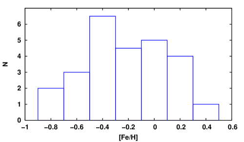
Figure 8: The distribution for the number ($N$) of objects, counted at 0.2 dex intervals, as a function of [Fe/H].

Based on an analysis of $JHK$ and $IRAS$ photometry of a large sample of Galactic symbiotic systems Whitelock & Munari (1992) argued that symbiotic giants could be related to the metal-rich M stars found in the Galactic bulge and elsewhere, i.e. that the symbiotic giants have low masses and higher than solar metallicity. They also noted that the mass-loss rates of the symbiotic giants, derived from the $K-[12]$ and $[25]-[12]$ colours, although systematically greater than for the local bright giants are similar to those of the bulge-like stars. Our abundance results, which is for a sample of southern symbiotic stars overlapping Whitelock & Munari’s sample, do not confirm the increased metallicity in symbiotic giants. On the contrary, we find subsolar metallicities that suggest efficient mass loss is needed to explain symbiotic activity. This is in line with conclusions from radio studies (Seaquist, Krogulec & Taylor 1993; Mikołajewska, Ivison & Omont 2002) that the symbiotic giants tend to have higher mass-loss rates than single giants of the same spectral type. Gromadzki, Mikołajewska & Soszyński (2013) found that light curves of most symbiotic systems have more or less regular variations with time-scales of 50–200 d, most likely due to stellar pulsations of the cool giant component. The presence of SRb variables in these systems can account for relatively high mass-loss rates from symbiotic giants, about a few times 10^-7 M_☉yr^-1, as compared with single field giants (Gromadzki et al., 2007b).

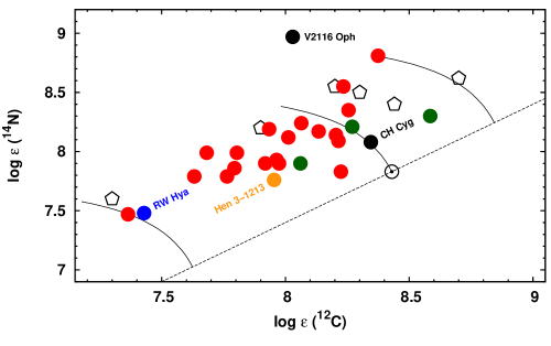
Figure 9: Nitrogen versus carbon for the symbiotic giants (circles). The dashed line represents scaled solar abundances, [¹²C/Fe] = 0 and [¹⁴N/Fe] = 0. The solid curves delineate constant ¹²C+¹⁴N. Bulge giants (Cunha & Smith, 2006) are shown as pentagons. Giants with highest ¹²C/¹³C $\geq 15$ (green circles, see Fig. 10) are less elevated in this plane, for instance CH Cyg with ¹²C$/^{13}$C = 18. See online edition for colour version.

The measured abundances of carbon, nitrogen, and oxygen are similar to values typical for single Galactic M giants (e.g. Smith & Lambert, 1990). In particular all our giants show an enhancement of nitrogen and a depletion of carbon. It is well known that during evolution on the red giant branch the abundances of carbon and nitrogen are changing because the CN cycle operates and extensive convection dredges nuclear processed material up to the outer layers. Simplifying, it can be assumed that only the CN cycle operates effectively in the stellar interior during this phase and thus ¹²C nuclei are converted mostly to ¹⁴N. As a result the ¹²C/¹⁴N ratio should be reduced with the total number of C+N nuclei conserved. The decrease in ¹²C combined with some increase in ¹³C nuclei results in a decrease in the ¹²C/¹³C ratio. This picture has been confirmed by a number of theoretical and observational studies and is called the ’first dredge-up’.

Evidence of the first dredge-up in our red giants is shown in Fig. 9. The abundances of ¹⁴N versus ¹²C for the symbiotic sample are shown compared to the abundances in Galactic bulge giants (Cunha & Smith, 2006) . All our symbiotic giants fall above the scaled solar line. This signifies an enhanced ¹⁴N abundance and indicates that the symbiotic giants have experienced the first dredge-up. The occurrence of the first dredge-up is also confirmed by the low ¹²C/¹³C isotopic ratios obtained for 10 objects (Fig. 10). We obtained ¹²C/¹³C values in the range 5–23 with average, and median, ¹²C/¹³C = $\sim$10. In Fig. 9 the position of our giants with highest ¹²C/¹³C ratio is less elevated in $\log{\mathrm{N}}$–$\log{\mathrm{C}}$ plane similar to CH Cyg for which Schmidt et al. (2006) obtained ¹²C$/^{13}$C = 18.

In Fig. 10 our high-resolution determinations of ¹²C/¹³C are compared to [C/H] reported in our papers as well as previous results derived by Schmidt & Mikołajewska (2003) and Schild, Boyle & Schmid (1992). The Schmidt & Mikołajewska (2003) and Schild, Boyle & Schmid (1992) results are based on spectra at significantly lower resolution. The low-resolution spectra which lack measurable CN molecular lines could not provide a good measure of carbon abundances. The underestimation of the carbon abundance is clearly visible in the case of CH Cyg and SY Mus (arrows in Fig. 10). The conclusion is that those abundances from low-resolution spectra are not suitable for comparison with theoretical models.

Lü et al. (2008) performed the first theoretical study of the chemical abundances in symbiotic giants. Among the elements studied are CNO abundances and ¹²C/¹³C isotopic ratio. The confrontation of observational ¹²C/¹³C and [C/H] with results of theoretical calculations shows that first dredge-up is insufficient to explain observed carbon abundances (Fig. 11). Lü et al. (2008) suggested that some additional mixing process, for instance thermohaline mixing applicable to low-mass giants (Charbonnel & Zahn, 2007), is required to model the measurements. However, Lü et al. (2008) used the solar initial composition in their calculations and did not consider the effect of metallicity on the carbon abundances. Our sample is not homogeneous in respect of [Fe/H] and it is dominated by objects with subsolar metallicities.

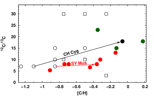
Figure 10: Chemical abundance ratio of ¹²C/¹³C versus [C/H] measured from $K_{\rm r}$-band spectra for 10 objects in our sample (red and green filled circles). CH Cyg from high-resolution spectra (Schmidt et al., 2006), black circle, from low-resolution spectra (Schild, Boyle & Schmid, 1992; Schmidt & Mikołajewska, 2003), open circles, and squares, respectively. See online edition for colour version.

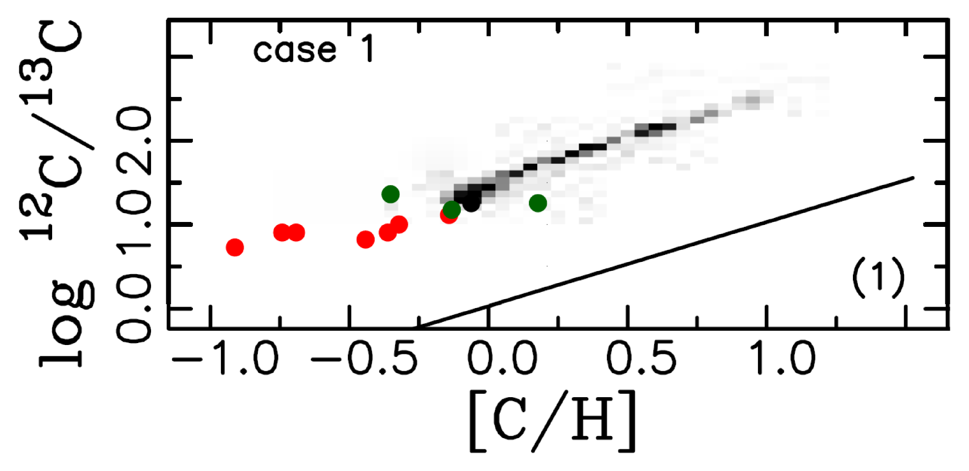
Figure 11: ¹²C/¹³C versus [C/H] from high-resolution spectra compared with one selected case (fig. 2, left, case 1) derived by Lü et al. (2008) from theoretical abundances. See online edition for colour version.

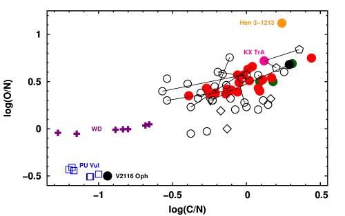
Figure 12: O/N versus C/N from the current photospheric abundances (filled symbols) compared with values from nebular lines (open symbols), Nussbaumer et al. (1988, circles), Schmid & Schild (1990, diamonds), Pereira (1995, pentagons) for KX TrA, Schmidt et al. (2006, triangle) for CH Cyg, and Vogel & Nussbaumer (1992, squares) for PU Vul during outburst. Crosses represent theoretical predictions for nova ejecta from CO WD with 0.65 M☉  (Kovetz & Prialnik, 1997). Solid lines link measurements obtained with two methods (from nebular lines and photospheric) for the same objects. See online edition for colour version.

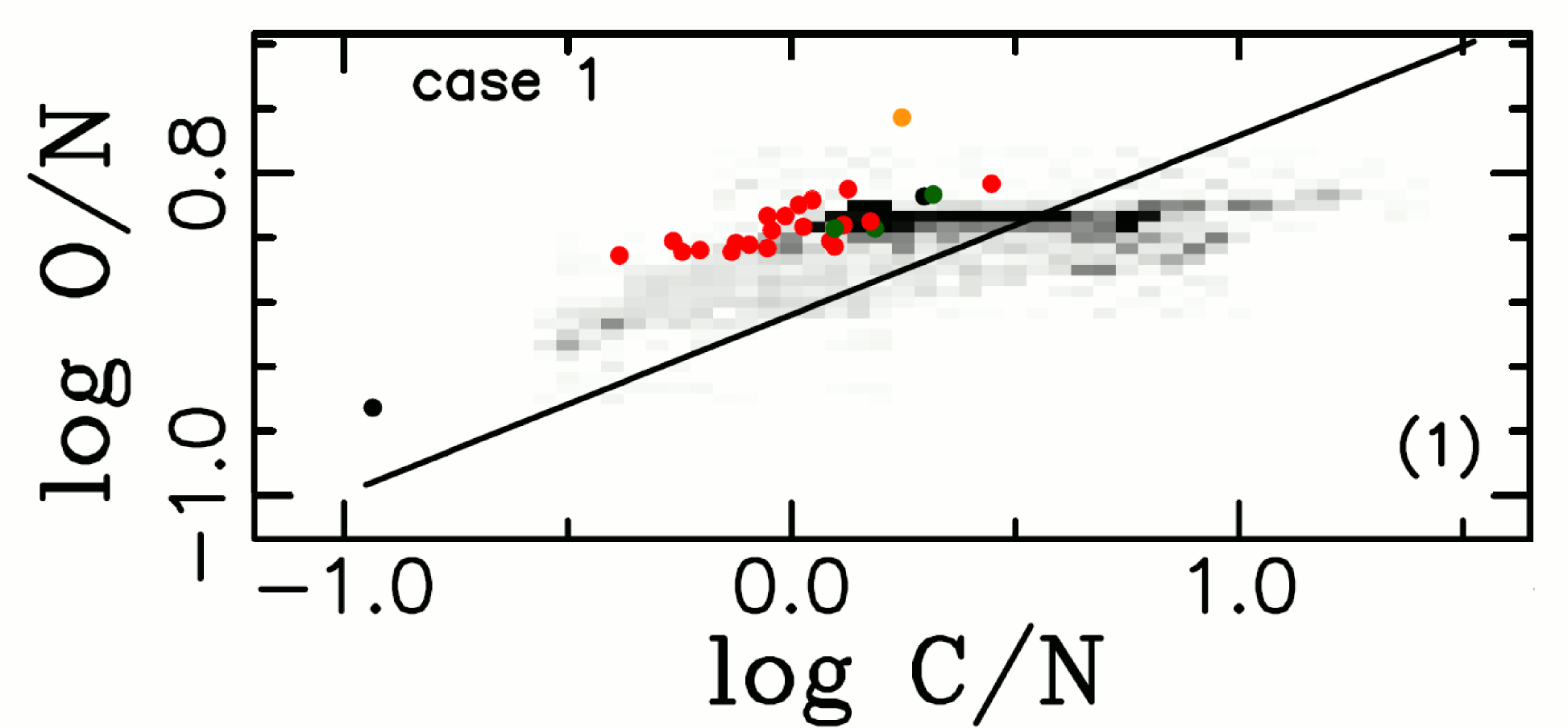
Figure 13: Comparison of observational $\log{\rm{O/N}}$ versus $\log{\rm{C/N}}$ (Fig. 12) with one selected theoretical case (fig. 3, left, case 1) derived by Lü et al. (2008). See online edition for colour version.

Most previous studies of C/N/O abundances in symbiotic systems have been based on nebular emission lines. In Fig. 12 O/N and C/N ratios obtained from photospheric abundances are compared with those from nebular lines (Nussbaumer et al. 1988; Schmid & Schild 1990; Vogel & Nussbaumer 1992; Pereira 1995; Schmidt et al. 2006). The nebular line results are more scattered in both of the coordinate directions. In part this could result from the larger uncertainty in the abundances derived from the nebular lines. A larger concern is changes in the measured abundances resulting from changes of physical conditions in the nebulae. In Fig. 12 the ’nebular’ points are shifted as a whole with respect to the ’photospheric’ points with the nebular points shifted to lower O/N and C/N ratios. The shift is towards the abundance ratios characterized by the symbiotic nebulae in outburst. As an example, the position of PU Vul during outburst, and the theoretical O/N and C/N ratios in ejecta from a 0.65 M☉CO white dwarf during nova outburst (Kovetz & Prialnik, 1997) are shown in Fig. 12.

The abundances of most symbiotic nebulae are between those of the cool giants and the materials ejected by the hot companions during symbiotic novae. The abundances measured from nebular lines can systematically underestimate the C and O abundances relative to the N abundance. Nussbaumer et al. (1988) noted that this effect could reach up to $\sim$30%. Another problem is that the emission spectrum depends significantly on the spatial orientation of the system. The abundances measured from emission lines change with orbital phase (eg. KX TrA in Fig. 12 shows the different values at orbital phases 0.52 and 0.27, see table 8 in Paper II). Reliable values can be obtained only with spectra taken during superior conjunction of the cool giant (see Paper II). Summarizing, the behaviour of nebular lines is useful for studying conditions in the circumbinary environment, for instance the conditions as a function of the changing projection of the system with orbital phase. The nebular lines can also be used to study the heating and supplying a new gas content as a result of thermonuclear explosions on the white dwarf.

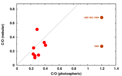
Figure 14: Nebular versus photospheric C/O ratios for objects with both values measured. The changing position of LMC S63 is shown.

Lü et al. (2008) conducted a theoretical analysis of O/N and C/N ratios in symbiotic giants. They considered specific regions in the O/N versus C/N diagram depending on whether or not the cool components have undergone the third dredge-up. The occurrence of the third dredge-up in evolved giants is a function of mass. Since the third dredge-up enriches envelopes with carbon and oxygen the relative abundances of O/N and C/N can constrain the masses of the giants. The location of our objects in the $\log{\rm{O/N}}$–$\log{\rm{C/N}}$ spaces defined by Lü et al. (2008) (Fig. 13, C/N $<$ O/N) suggests that the cool components of our symbiotic systems are low-mass giants ($M<$ 4M☉) that have not undergone or have undergone only inefficient third dredge-up. The special location of V2116 Oph, at the bottom region of C/N $<$ O/N (Fig. 13), may suggest that it could be the only symbiotic giant that passed through third dredge-up and the hot bottom burning. However, this is precluded by the well-established, relatively low mass of this giant $M=$ 1.22M☉(Hinkle et al., 2006). The high N enrichment clearly visible in Figs 9, 12, and 13, and peculiar, in general, chemical composition of the red giant in V2116 Oph, must be the manifestation of past mass transfer from the more massive, evolved companion before it went through the supernova stage and became a neutron star.

Lü et al. (2008) also compared theoretical ratios with those of symbiotic nebulae, novae, and planetary nebulae. Lü et al. (2008) did not have photospheric C/N/O compositions for symbiotic giants. Now we can compare the photospheric O/N and C/N ratios with those from symbiotic nebulae and novae (Figs 12 and 13). It confirms previous suggestions that the compositions of the symbiotic nebulae are modified by the material ejected from the hot components during active phase. Thus, decreases in O/N, C/N, and C/O ratios occur. Following an active phase the abundances return slowly to the state that existed before activity as material in nebula becomes dominated by material from the red giant wind. The wind material is rich mainly in oxygen and/or carbon. A good example is symbiotic S63 in LMC where C/O ratio seems to grow continuously (Fig. 14) after active phases (Iłkiewicz et al., 2015).

When the evolution of carbon and nitrogen abundances occurs with the total number of carbon plus nitrogen nuclei conserved it can be presumed that the oxygen abundance should remain almost unchanged. In such cases we can assume, as did Cunha & Smith (2006), that the oxygen abundance is still roughly the value with which the star was born. Oxygen is one of the $\alpha$-elements that are particularly important in studying the evolution of stars in the context of the formation and chemical evolution of Galactic populations. In our sample giants we measured abundances of two $\alpha$-elements, oxygen and titanium. The $\alpha$-elements are produced over relatively short time-scales, originating mostly from massive stars and Type II supernovae (SNe II). Iron, on the other hand, is produced over much longer time-scales in the Type Ia supernovae (SNe Ia) explosions. The contamination of the interstellar medium (ISM) with material originated from these two sources can lead to significantly different trends for particular populations. Thus, clear separations between sequences for various stellar populations are observed in the [O$/$Fe] versus [Fe$/$H] and [Ti$/$Fe] versus [Fe$/$H] planes (see e.g. Bensby & Feltzing 2006; Cunha & Smith 2006).

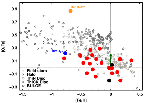
Figure 15: Oxygen relative to iron for various stellar populations with positions of our targets denoted with large coloured circles. Four populations are distinguished: thin and thick discs, halo, and bulge. The thin and thick disc samples contain only those objects with membership confirmed by their kinematic characteristics. A large black circles marks the positions of CH Cyg (top) from Schmidt et al. (2006) and V2116 Oph (bottom) the symbiotic neutron star system from (Hinkle et al., 2006). The green arrow denotes the systematic shift from the use of PHOENIX models instead of MARCS models (see Section 4). See online edition for colour version.

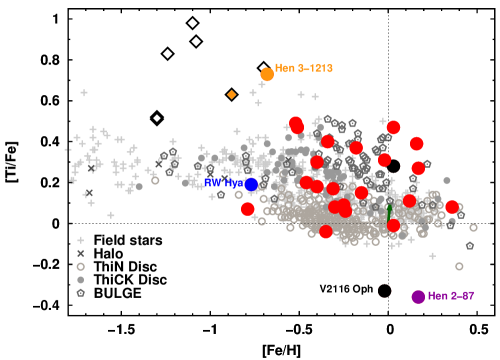
Figure 16: Titanium relative to iron for various stellar populations with positions of our targets denoted with large coloured circles. Symbols analogous to those in Fig. 15. Black open diamonds are giants in yellow symbiotic systems from Smith et al. 1996, 1997, Pereira, Smith & Cunha 1998, and Pereira & Roig 2009. Yellow open diamond are Ti and Fe abundances from Pereira & Roig (2009) for Hen 3-1213. Hen 2-87 (magenta) has a particularly very low [Ti$/$Fe] ratio. See online edition for colour version.

We use our values for the abundances of oxygen, iron, and titanium in 24 symbiotic giants to investigate the first analyses of symbiotics in term of chemical evolution and membership in Galactic populations. Figs 15 and 16 show [O$/$Fe] and [Ti$/$Fe], respectively, as a function of [Fe$/$H] for the symbiotic giants along with values for various stellar populations (halo, thin and thick disc, and bulge) from the literature (Gratton & Sneden 1988; Edvardsson et al. 1993; McWilliam et al. 1995; Fulbright 2000; Prochaska, Naumov & Carney 2000; Boyarchuk et al. 2001; Mélendez, Barbuy & Spite 2001; Smith, Cunha & King 2001; Johnson 2002; Mélendez & Barbuy 2002; Fulbright & Johnson 2003; Reddy et al. 2003; Bensby et al. 2005; Rich & Origlia 2005; Cunha & Smith 2006; Alves-Brito et al. 2010; Ryde et al. 2010; Bensby et al. 2011; Rich, Origlia & Valenti 2012; Smith et al. 2013). The population studies have been scaled to the solar composition of Asplund et al. (2009) for CNO, and Scott et al. (2015) for elements around the iron peak (Fe and Ti). The halo, thin- and thick-disc populations are grouped around clear sequences. On the contrary, the bulge population seems be composed of a more or less chemically inhomogeneous groups of stars. It is more scattered in the [O$/$Fe] versus [Fe$/$H] (see Paper II) and [Ti$/$Fe] versus [Fe$/$H] planes overlapping partly with all other populations. It is, however, in both cases shifted somewhat towards higher [O$/$Fe] and [Ti$/$Fe] perhaps reflecting more rapid enrichment in metals from SNe II explosions (see Cunha & Smith, 2006). In the [O$/$Fe] versus [Fe$/$H] diagram (Fig. 15) most of our targets are located on or somewhat below of area occupied by thin- and thick-disc populations. The position of RW Hya and Hen 3-1213 at low metallicity, [Fe$/$H]$\sim$-0.8, supports their membership in the extended thick-disc/halo population.

Pereira & Roig (2009) from their analysis of four yellow symbiotic systems, including Hen 3-1213, concluded that the overall abundance pattern follows the halo abundances. In the [Ti$/$Fe]–[Fe$/$H] plane (Fig. 16) our M-type giants are typically at higher [Ti$/$Fe] in a region occupied mainly by thick-disc and bulge stars. The only yellow symbiotic in our sample, Hen 3-1213, has even higher [Ti$/$Fe]. Similar enhancement of [Ti$/$Fe] was found by Pereira & Roig (2009) for yellow symbiotic giants. They also noticed that the other $\alpha$-elements to Fe are typical of halo giant stars of the same metallicity. We used the published [Ti$/$Fe] values for AG Dra (Smith et al., 1996), BD-21^∘3873 (Smith et al., 1997), Hen 2-467 (Pereira, Smith & Cunha, 1998), CD-43^∘14304, Hen 3-863, StH$\alpha$ 176, and Hen 3-1213 (Pereira & Roig, 2009) to plot their positions in Fig. 16. This plot demonstrates that this Ti anomaly increases with decreasing metallicity. The reason for such a high titanium abundance in symbiotic giants is not known and we are not able to provide any interpretation. However, Cunha & Smith (2006) noted very similar behaviour for their bulge giants. Our present results indicate that this titanium anomaly is present in both red (i.e. M-type giants) and yellow symbiotic systems. The data available are still relatively scant and noisy but we can speculate that this anomaly is distributed along a sequence, suggesting this is a genuine characteristic of S-type symbiotic giants.

6 Conclusions

Analysis of the photospheric abundances of CNO and elements around the iron peak (Fe, Ti, Ni, and Sc) was performed for the giant stars in a sample of 24 southern S-type symbiotic systems. Our analysis resulted in metallicities distributed in a wide range from significantly subsolar ([Fe$/$H]$\sim-0.8$ dex) to slightly supersolar ([Fe$/$H]$\sim+0.35$ dex), with largest representation around slightly subsolar ([Fe$/$H]$\sim-0.4$ to $-0.3$ dex) and near-solar metallicity. The enrichment in ¹⁴N isotope, found in all cases, indicates that the giants have experienced the first dredge-up. This is confirmed by the low ¹²C/¹³C ratio (5–23) that was measured in a subset of the sample. Comparison with abundances from nebular lines shows that the nebulae are contaminated by activity on the white dwarf and do not provide reliable abundances for the red giant. We found that the enhanced [Ti$/$Fe] abundances previously found for yellow symbiotic systems are also typically enhanced in red symbiotic giants. This suggests that enhanced [Ti$/$Fe] abundance could be a characteristic of the giants in S-type symbiotic systems.

Appendix A The full journal of spectroscopic observations.

Table 7: Journal of spectroscopic observations. Quadrature sums of the projected rotational velocities and microturbulence$\,{}^{a}$ $(V_{\mathrm{rot}}^{2}\sin^{2}{i}+\xi^{2}_{\mathrm{t}})^{0.5}$ shown have been obtained via cross-correlation technique (CCF) and from measurement of full width at half-maximum (FWHM) of $K$ band Ti i, Fe i, and Sc i absorption lines. Orbital phases have been calculated according to the referenced literature ephemeris.

	Id. num.b	Sp. region	Date	HJD(mid)	$(V_{\mathrm{rot}}^{2}\sin^{2}{i}+\xi^{2}_{\mathrm{t}})^{0.5}$		Orbital phasec
		band($\lambda$[µm])	(dd.mm.yyyy)		CCF	FWHM
		$H$ ($\sim$1.56)	16.02.2003	245 2686.7409	6.08	–	0.30
BX Mon	23	$K$ ($\sim$2.23)	20.04.2003	245 2749.5231	7.58	8.67 $\pm$ 1.41	0.35
		$K_{\rm r}$ ($\sim$2.36)	03.04.2006	245 3828.5095	8.44	–	0.20
						8.67 $\pm$ 1.41d
		$H$ ($\sim$1.56)	16.02.2003	245 2686.7491	4.19	–	0.39
V694 Mon	24	$K$ ($\sim$2.23)	20.04.2003	245 2749.5326	6.34	8.42 $\pm$ 0.99	0.42
		$K_{\rm r}$ ($\sim$2.36)	03.04.2006	245 3828.5187	7.21	–	0.98
		$H_{\rm b}$ ($\sim$1.54)	12.03.2010	245 5267.5052	9.36	–	0.72
						8.42 $\pm$ 0.99d
		$H$ ($\sim$1.56)	16.02.2003	245 2686.7769	3.97	–	0.98
Hen 3-461	31	$K$ ($\sim$2.23)	20.04.2003	245 2749.5662	7.42	8.18 $\pm$ 0.63	0.08
		$K$ ($\sim$2.23)	13.12.2003	245 2986.7827	7.38	7.11 $\pm$ 0.76	0.46
		$K$ ($\sim$2.23)	03.04.2004	245 3098.6078	6.54	7.66 $\pm$ 0.89	0.63
		$K_{\rm r}$ ($\sim$2.36)	03.04.2006	245 3828.5602	6.63	–	0.78
		$H$ ($\sim$1.56)	02.04.2009	245 4923.5570	4.68	–	0.50
		$H$ ($\sim$1.56)	23.05.2010	245 5340.4918	5.24	–	0.16
						7.68 $\pm$ 0.52d
		$H$ ($\sim$1.56)	17.02.2003	245 2687.7566	3.88	–	0.02
SY Mus	33	$K$ ($\sim$2.23)	20.04.2003	245 2749.5817	5.98	6.91 $\pm$ 0.99	0.12
		$K$ ($\sim$2.23)	13.12.2003	245 2986.8250	6.84	6.97 $\pm$ 0.98	0.50
		$K_{\rm r}$ ($\sim$2.36)	03.04.2006	245 3828.5767	5.01	–	0.84
		$H$ ($\sim$1.56)	02.04.2009	245 4923.5906	5.60	–	0.60
		$H_{\rm b}$ ($\sim$1.54)	23.03.2010	245 5278.5907	5.84	–	0.16
		$H$ ($\sim$1.56)	26.04.2010	245 5312.6012	6.53	–	0.22
						6.94 $\pm$ 0.64d
		$H$ ($\sim$1.56)	17.02.2003	245 2687.7725	5.01	–	–
Hen 2-87	37	$K$ ($\sim$2.23)	20.04.2003	245 2749.5942	7.80	9.13 $\pm$ 0.76	–
		$K$ ($\sim$2.23)	13.12.2003	245 2986.8410	10.62	10.28 $\pm$ 1.42	–
		$K$ ($\sim$2.23)	03.04.2004	245 3098.6172	8.84	10.09 $\pm$ 0.82	–
		$K_{\rm r}$ ($\sim$2.36)	03.04.2006	245 3828.5853	8.73	–	–
		$H$ ($\sim$1.56)	24.04.2010	245 5310.6015	6.53	–	–
						9.79 $\pm$ 0.66d
		$H$ ($\sim$1.56)	16.02.2003	245 2686.8053	3.64	–	–
Hen 3-828	38	$K$ ($\sim$2.23)	20.04.2003	245 2749.6031	8.03	8.29 $\pm$ 1.07	–
		$K$ ($\sim$2.23)	13.12.2003	245 2986.8478	7.66	7.75 $\pm$ 0.82	–
		$K$ ($\sim$2.23)	03.04.2004	245 3098.6278	6.62	8.43 $\pm$ 0.72	–
		$K_{\rm r}$ ($\sim$2.36)	03.04.2006	245 3828.6050	7.39	–	–
						8.17 $\pm$ 0.54d
		$H$ ($\sim$1.56)	16.02.2003	245 2686.8181	6.94	–	–
CD-36∘8436	42	$K$ ($\sim$2.23)	20.04.2003	245 2749.6156	6.96	8.37 $\pm$ 1.11	–
		$K_{\rm r}$ ($\sim$2.36)	03.04.2006	245 3828.6211	6.45	–	–
		$H_{\rm b}$ ($\sim$1.54)	15.03.2010	245 5270.8938	7.91	–	–
		$H$ ($\sim$1.56)	24.04.2010	245 5310.6144	8.81	–	–
						8.37 $\pm$ 1.11d

• phases are calculated from the following ephemerides: BX Mon 2449796+1259$\times$E (Fekel et al., 2000), V694 Mon 2448080+1931$\times$E (Gromadzki et al., 2007a), Hen 3-461 2452063+635$\times$E (Gromadzki, Mikołajewska & Soszyński, 2013), SY Mus 2450176+625$\times$E (Dumm et al., 1999), RW Hya 2445071.6+370.2$\times$E (Kenyon & Mikołajewska, 1995) or 2449512+370.4$\times$E (Schild, Mürset & Schmutz, 1996), Hen 3-916 2452410+803$\times$E (Gromadzki, Mikołajewska & Soszyński, 2013), Hen 3-1213 2451806+514$\times$E (Gromadzki, Mikołajewska & Soszyński, 2013), Hen 2-173 2452625+911$\times$E (Fekel et al., 2007). KX TrA 2453053+1350$\times$E (Ferrer et al., 2003), CL Sco 2452018+625$\times$E (Fekel et al., 2007), V455 Sco 2452641.5+1398$\times$E (Fekel et al., 2008), Hen 2-247 2452355+898$\times$E (Fekel et al., 2008), AE Ara 2453449+803.4$\times$E (Fekel et al., 2010), AS 270 2451633+671$\times$E (Fekel et al., 2007), Y CrA 2454126+1619$\times$E (Fekel et al., 2010), Hen 2-374 2453173+820$\times$E (Fekel et al., 2010).

• $(V_{\mathrm{rot}}^{2}\sin^{2}{i}+\xi^{2}_{\mathrm{t}})^{0.5}$ obtained from all $K$-band spectra jointly – used for synthetic spectra calculations.

Table 8: continued

	Id. num.b	Sp. region	Date	HJD (mid)	$(V_{\mathrm{rot}}^{2}\sin^{2}{i}+\xi^{2}_{\mathrm{t}})^{0.5}$		Orbital phasec
		band($\lambda$[µm])	(dd.mm.yyyy)		CCF	FWHM
		$H$ ($\sim$1.56)	16.02.2003	245 2686.8380	5.74	–	0.57
RW Hya	45	$K$ ($\sim$2.23)	20.04.2003	245 2749.6295	6.63	6.73 $\pm$ 1.80	0.74
		$K$ ($\sim$2.23)	13.12.2003	245 2986.8656	6.25	6.35 $\pm$ 0.72	0.38
		$K_{\rm r}$ ($\sim$2.36)	03.04.2006	245 3828.6308	5.57	–	0.65
		$H$ ($\sim$1.56)	24.04.2010	245 5310.5915	8.80	–	0.66
						6.54 $\pm$ 0.94d
		$K$ ($\sim$2.23)	20.04.2003	245 2749.6619	8.19	8.34 $\pm$ 1.17	0.42
Hen 3-916	46	$K$ ($\sim$2.23)	03.04.2004	245 3098.6407	8.78	9.11 $\pm$ 1.30	0.86
		$K_{\rm r}$ ($\sim$2.36)	03.04.2006	245 3828.6583	8.38	–	0.77
		$H$ ($\sim$1.56)	26.04.2010	245 5312.5667	6.73	–	0.62
		$H$ ($\sim$1.56)	22.05.2010	245 5338.5624	7.98	–	0.65
						8.69 $\pm$ 0.90d
		$H$ ($\sim$1.56)	17.02.2003	245 2687.7791	5.29	–	–
Hen 3-1092	53	$K$ ($\sim$2.23)	03.04.2004	245 3098.6669	5.80	6.16 $\pm$ 0.79	–
		$H$ ($\sim$1.56)	26.04.2010	245 5312.6269	5.26	–	–
						6.16 $\pm$ 0.79d
		$H$ ($\sim$1.56)	17.02.2003	245 2687.7936	5.97	–	–
WRAY 16-202	59	$K$ ($\sim$2.23)	20.04.2003	245 2749.7301	6.60	8.54 $\pm$ 1.67	–
		$K_{\rm r}$ ($\sim$2.36)	03.04.2006	245 3828.6812	8.39	–	–
		$H$ ($\sim$1.56)	24.04.2010	245 5310.6498	6.17	–	–
						8.54 $\pm$ 1.67d
		$H$ ($\sim$1.56)	16.02.2003	245 2686.8581	9.89	–	0.71
Hen 3-1213	65	$K$ ($\sim$2.23)	20.04.2003	245 2749.7403	7.24	7.82 $\pm$ 0.59	0.84
		$K$ ($\sim$2.23)	14.08.2003	245 2866.4846	8.38	7.60 $\pm$ 0.69	0.06
		$K$ ($\sim$2.23)	03.04.2004	245 3098.6892	9.43	7.68 $\pm$ 0.41	0.52
		$H$ ($\sim$1.56)	24.05.2010	245 5340.5865	11.76	–	0.88
						7.70 $\pm$ 0.30d
		$H$ ($\sim$1.56)	16.02.2003	245 2686.8989	6.36	–	0.07
Hen 2-173	66	$K$ ($\sim$2.23)	20.04.2003	245 2749.7497	7.38	8.31 $\pm$ 1.29	0.14
		$K$ ($\sim$2.23)	14.08.2003	245 2866.4998	9.06	8.27 $\pm$ 0.57	0.27
		$K$ ($\sim$2.23)	03.04.2004	245 3098.7025	8.15	9.34 $\pm$ 0.81	0.52
		$H$ ($\sim$1.56)	24.05.2010	245 5340.5508	7.50	–	0.98
						8.64 $\pm$ 0.65d
		$H$ ($\sim$1.56)	17.02.2003	245 2687.8230	6.05	–	0.73
KX TrA	68	$K$ ($\sim$2.23)	20.04.2003	245 2749.7670	6.29	8.48 $\pm$ 1.77	0.78
		$K$ ($\sim$2.23)	03.04.2004	245 3098.7314	5.74	8.94 $\pm$ 2.12	0.03
		$H$ ($\sim$1.56)	24.05.2010	245 5340.6039	6.58	–	0.69
						8.71 $\pm$ 1.32d
		$H$ ($\sim$1.56)	17.02.2003	245 2687.8341	7.02	–	0.07
CL Sco	71	$K$ ($\sim$2.23)	20.04.2003	245 2749.7780	6.99	7.84 $\pm$ 1.78	0.17
		$K$ ($\sim$2.23)	15.08.2003	245 2866.5367	8.52	8.02 $\pm$ 1.62	0.36
		$K$ ($\sim$2.23)	03.04.2004	245 3098.7794	8.83	8.42 $\pm$ 1.48	0.73
						8.09 $\pm$ 0.87d
		$H$ ($\sim$1.56)	17.02.2003	245 2687.8626	5.23	–	0.03
V455 Sco	73	$K$ ($\sim$2.23)	20.04.2003	245 2749.7874	7.78	8.62 $\pm$ 1.63	0.08
		$K$ ($\sim$2.23)	03.04.2004	245 3098.7959	7.40	8.65 $\pm$ 1.30	0.33
		$H$ ($\sim$1.56)	24.05.2010	245 5340.6339	7.25	–	0.93
						8.63 $\pm$ 0.98d
		$H$ ($\sim$1.56)	17.02.2003	245 2687.8745	7.28	–	0.37
Hen 2-247	88	$K$ ($\sim$2.23)	20.04.2003	245 2749.8453	9.53	11.47 $\pm$ 1.07	0.44
		$K$ ($\sim$2.23)	15.08.2003	245 2866.5144	10.95	11.29 $\pm$ 0.68	0.57
		$K$ ($\sim$2.23)	03.04.2004	245 3098.8329	7.69	9.21 $\pm$ 1.55	0.83
		$H$ ($\sim$1.56)	27.06.2010	245 5374.7414	7.97	–	0.36
						10.58 $\pm$ 1.05d
RT Ser	92	$K$ ($\sim$2.23)	20.04.2003	245 2749.8550	6.22	8.10 $\pm$ 1.78	–
						8.10 $\pm$ 1.78d

Table 9: continued

	Id. num.b	Sp. region	Date	HJD (mid)	$(V_{\mathrm{rot}}^{2}\sin^{2}{i}+\xi^{2}_{\mathrm{t}})^{0.5}$		Orbital phasec
		band($\lambda$[µm])	(dd.mm.yyyy)		CCF	FWHM
		$H$ ($\sim$1.56)	17.02.2003	245 2687.8830	7.76	–	0.05
AE Ara	93	$K$ ($\sim$2.23)	20.04.2003	245 2749.8669	9.16	10.06 $\pm$ 0.96	0.13
		$K$ ($\sim$2.23)	03.04.2004	245 3098.8487	10.35	10.58 $\pm$ 1.42	0.56
						10.30 $\pm$ 0.83d
		$K$ ($\sim$2.23)	20.04.2003	245 2749.9407	10.68	9.25 $\pm$ 0.71	–
SS73 96	94	$K$ ($\sim$2.23)	03.04.2004	245 3098.8573	8.47	9.30 $\pm$ 0.66	–
		$H$ ($\sim$1.56)	02.06.2010	245 5349.6673	7.07	–	–
						9.28 $\pm$ 0.46d
		$H$ ($\sim$1.56)	17.02.2003	245 2687.8917	6.66	–	0.57
AS 270	119	$K$ ($\sim$2.23)	03.04.2004	245 3098.8687	8.77	10.23 $\pm$ 0.90	0.19
		$H$ ($\sim$1.56)	24.05.2010	245 5340.9087	8.28	–	0.53
						10.23 $\pm$ 0.90d
		$K$ ($\sim$2.23)	20.04.2003	245 2749.8760	9.56	10.57 $\pm$ 2.92	0.15
Y CrA	131	$H$ ($\sim$1.56)	31.07.2009	245 5043.7660	5.67	–	0.57
						10.57 $\pm$ 2.92d
Hen 2-374	136	$K$ ($\sim$2.23)	03.04.2004	245 3098.8781	5.98	6.66 $\pm$ 0.56	0.91
						6.66 $\pm$ 0.56d
		$K$ ($\sim$2.23)	15.08.2003	245 2866.5289	7.57	7.18 $\pm$ 1.02	–
Hen 3-1761	170	$K$ ($\sim$2.23)	03.04.2004	245 3098.9345	6.38	7.27 $\pm$ 0.59	–
		$H$ ($\sim$1.56)	06.06.2009	245 4988.9189	6.68	–	–
		$H$ ($\sim$1.56)	03.06.2010	245 5350.7945	5.25	–	–
						7.22 $\pm$ 0.63d

Appendix B Spectra of 24 symbiotic giants observed in $H$-, and/or $H_{\rm b}$-, $K$-, $K_{\rm r}$-band regions, compared with synthetic fits

Figure 17: The $H$-band spectrum of BX Mon observed 2003 February (blue line) and a synthetic spectrum (red line) calculated using the final abundances and ¹²C/¹³C isotopic ratio (Table 4).

Figure 19: The $K_{\rm r}$-band spectrum of BX Mon observed 2006 April (blue line) and a synthetic spectrum (red line) calculated using the final abundances and ¹²C/¹³C isotopic ratio (Table 4).

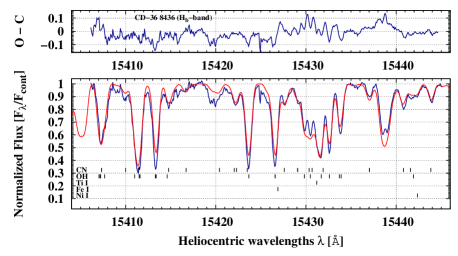
Figure 38: The $H_{\rm b}$-band spectrum of CD-36^∘8436 observed 2010 March (blue line) and a synthetic spectrum (red line) calculated using the final abundances and ¹²C/¹³C isotopic ratio (Table 4).

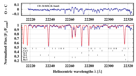
Figure 39: The $K$-band spectrum of CD-36^∘8436 observed 2003 April (blue line) and a synthetic spectrum (red line) calculated using the final abundances and ¹²C/¹³C isotopic ratio (Table 4).

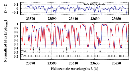
Figure 40: The $K_{\rm r}$-band spectrum of CD-36^∘8436 observed 2006 April (blue line) and a synthetic spectrum (red line) calculated using the final abundances and ¹²C/¹³C isotopic ratio (Table 4).

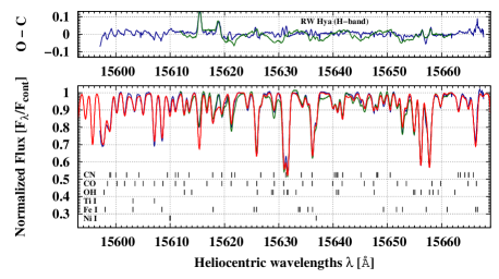
Figure 41: $H$-band spectra of RW Hya observed 2003 February (blue line), 2010 April (green line), and a synthetic spectrum (red line) calculated using the final abundances and ¹²C/¹³C isotopic ratio (Table 4).

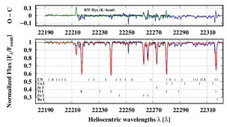
Figure 42: $K$-band spectra of RW Hya observed 2003 April (blue line), 2003 December (green line), and a synthetic spectrum (red line) calculated using the final abundances (Table 4).

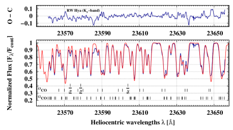
Figure 43: The $K_{\rm r}$-band spectrum of RW Hya observed 2006 April (blue line) and a synthetic spectrum (red line) calculated using the final abundances and ¹²C/¹³C isotopic ratio (Table 4).

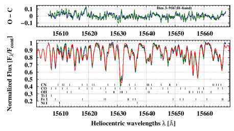
Figure 44: $H$-band spectra of Hen 3-916 observed 2010 April (blue line), 2010 May (green line), and a synthetic spectrum (red line) calculated using the final abundances and ¹²C/¹³C isotopic ratio (Table 4).

Figure 45: $K$-band spectra of Hen 3-916 observed 2003 April (blue line), 2004 April (green line), and a synthetic spectrum (red line) calculated using the final abundances (Table 4).

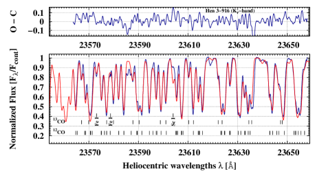
Figure 46: The $K_{\rm r}$-band spectrum of Hen 3-916 observed 2006 April (blue line) and a synthetic spectrum (red line) calculated using the final abundances and ¹²C/¹³C isotopic ratio (Table 4).

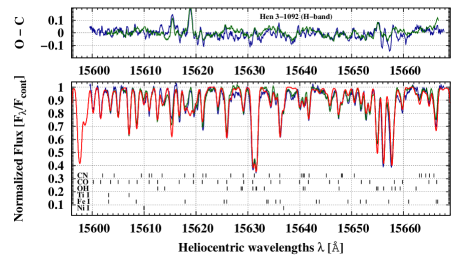
Figure 47: $H$-band spectra of Hen 3-1092 observed 2003 February (blue line), 2010 April (green line), and a synthetic spectrum (red line) calculated using the final abundances (Table 4).

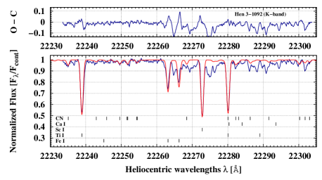
Figure 48: The $K$-band spectrum of Hen 3-1092 observed 2004 April (blue line) and a synthetic spectrum (red line) calculated using the final abundances (Table 4).

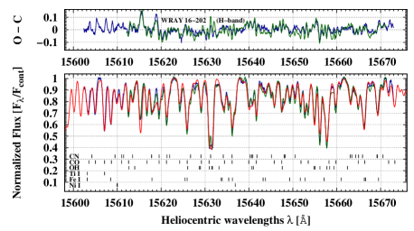
Figure 49: $H$-band spectra of WRAY 16-202 observed 2003 February (blue line), 2010 April (green line), and a synthetic spectrum (red line) calculated using the final abundances and ¹²C/¹³C isotopic ratio (Table 4).

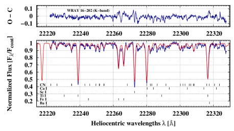
Figure 50: The $K$-band spectrum of WRAY 16-202 observed 2003 April (blue line) and a synthetic spectrum (red line) calculated using the final abundances and ¹²C/¹³C isotopic ratio (Table 4).

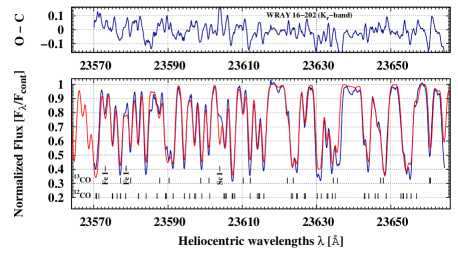
Figure 51: The $K_{\rm r}$-band spectrum of WRAY 16-202 observed 2006 April (blue line) and a synthetic spectrum (red line) calculated using the final abundances and ¹²C/¹³C isotopic ratio (Table 4).

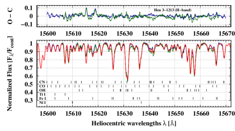
Figure 52: $H$-band spectra of Hen 3-1213 observed 2003 February (blue line), 2010 May (green line), and a synthetic spectrum (red line) calculated using the final abundances (Table 4).

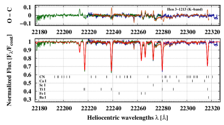
Figure 53: $K$-band spectra of Hen 3-1213 observed 2003 April (blue line), 2003 August (green line), 2004 April (dark-orange line), and a synthetic spectrum (red line) calculated using the final abundances (Table 4).

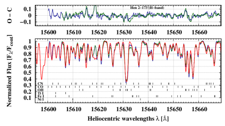
Figure 54: $H$-band spectra of Hen 2-173 observed 2003 February (blue line), 2010 May (green line), and a synthetic spectrum (red line) calculated using the final abundances (Table 4).

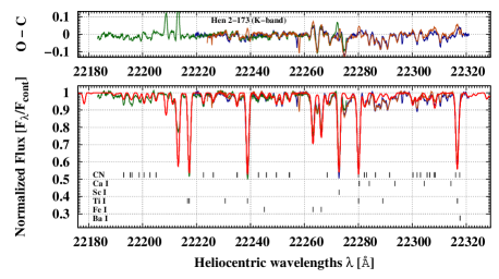
Figure 55: $K$-band spectra of Hen 2-173 observed 2003 April (blue line), 2003 August (green line), 2004 April (dark-orange line), and a synthetic spectrum (red line) calculated using the final abundances (Table 4).

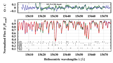
Figure 56: $H$-band spectra of KX TrA observed 2003 February (blue line), 2010 May (green line), and a synthetic spectrum (red line) calculated using the final abundances (Table 4).

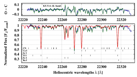
Figure 57: $K$-band spectra of KX TrA observed 2003 April (blue line), 2004 April (green line), and a synthetic spectrum (red line) calculated using the final abundances (Table 4).

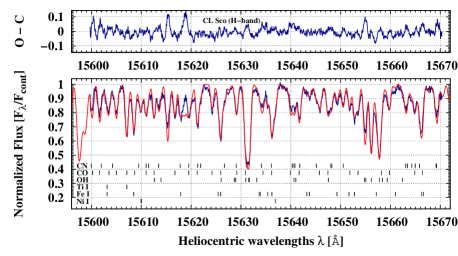
Figure 58: The $H$-band spectrum of CL Sco observed 2003 February (blue line) and a synthetic spectrum (red line) calculated using the final abundances (Table 4).

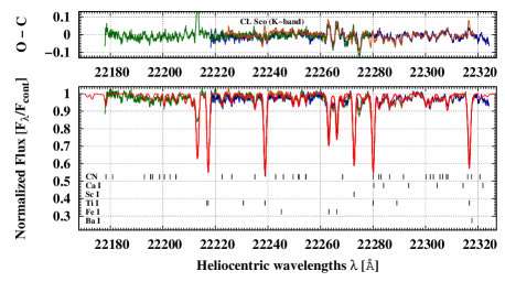
Figure 59: $K$-band spectra of CL Sco observed 2003 April (blue line), 2003 August (green line), 2004 April (dark-orange line), and a synthetic spectrum (red line) calculated using the final abundances (Table 4).

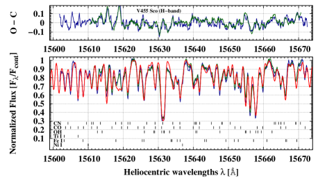
Figure 60: $H$-band spectra of V455 Sco observed 2003 February (blue line), 2010 May (green line), and a synthetic spectrum (red line) calculated using the final abundances (Table 4).

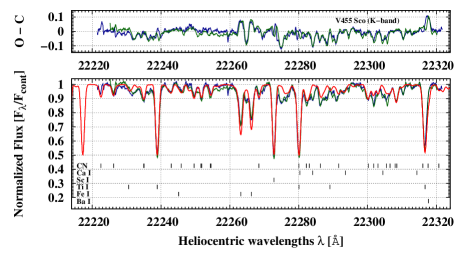
Figure 61: $K$-band spectra of V455 Sco observed 2003 April (blue line), 2004 April (green line), and a synthetic spectrum (red line) calculated using the final abundances (Table 4).

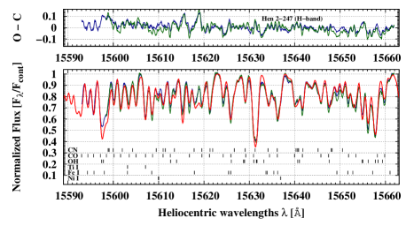
Figure 62: $H$-band spectra of Hen 2-247 observed 2003 February (blue line), 2010 June (green line), and a synthetic spectrum (red line) calculated using the final abundances (Table 4).

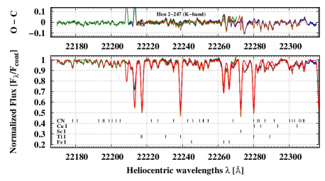
Figure 63: $K$-band spectra of Hen 2-247 observed 2003 April (blue line), 2003 August (green line), 2004 April (dark-orange line), and a synthetic spectrum (red line) calculated using the final abundances (Table 4).

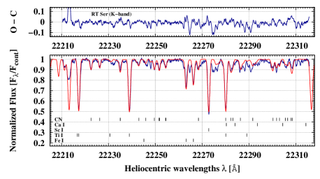
Figure 64: The $K$-band spectrum of RT Ser observed 2003 April (blue line) and a synthetic spectrum (red line) calculated using the final abundances (Table 4).

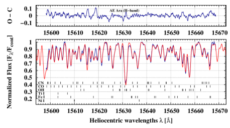
Figure 65: The $H$-band spectrum of AE Ara observed 2003 February (blue line) and a synthetic spectrum (red line) calculated using the final abundances (Table 4).

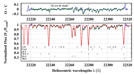
Figure 66: $K$-band spectra of AE Ara observed 2003 April (blue line), 2004 April (green line), and a synthetic spectrum (red line) calculated using the final abundances (Table 4).

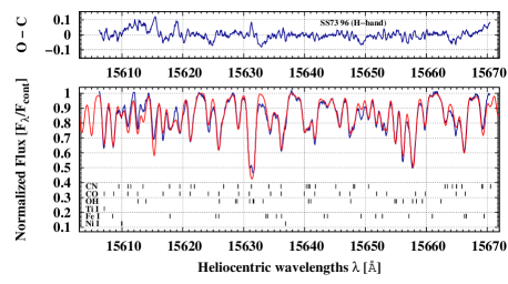
Figure 67: The $H$-band spectrum of SS73 96 observed 2010 June (blue line) and a synthetic spectrum (red line) calculated using the final abundances (Table 4).

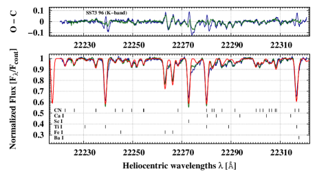
Figure 68: $K$-band spectra of SS73 96 observed 2003 April (blue line), 2004 April (green line), and a synthetic spectrum (red line) calculated using the final abundances (Table 4).

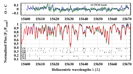
Figure 69: $H$-band spectrum of AS 270 observed 2003 February (blue line), 2010 May (green line), and a synthetic spectrum (red line) calculated using the final abundances (Table 4).

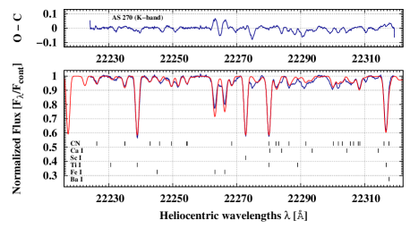
Figure 70: The $K$-band spectrum of AS 270 observed 2004 April (blue line) and a synthetic spectrum (red line) calculated using the final abundances (Table 4).

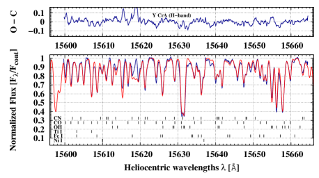
Figure 71: The $H$-band spectrum of Y CrA observed 2009 July (blue line) and a synthetic spectrum (red line) calculated using the final abundances (Table 4).

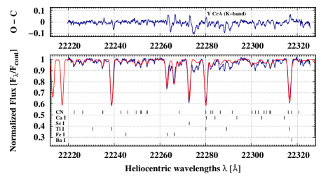
Figure 72: The $K$-band spectrum of Y CrA observed 2003 April (blue line) and a synthetic spectrum (red line) calculated using the final abundances (Table 4).

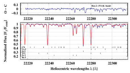
Figure 73: The $K$-band spectrum of Hen 2-374 observed 2004 April (blue line) and a synthetic spectrum (red line) calculated using the final abundances (Table 4).

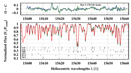
Figure 74: $H$-band spectra of Hen 3-1761 observed 2009 June (blue line), 2010 June (green line), and a synthetic spectrum (red line) calculated using the final abundances (Table 4).

References

- Allen (1980) Allen D. A., 1980, MNRAS, 192, 521
- Alvarez & Plez (1998) Alvarez R., Plez B., 1998, A&A, 330, 1109
- Alves-Brito et al. (2010) Alves-Brito A., Meléndez J., Asplund M., Ramírez I., Yong D., 2010, A&A, 513, 35
- Asplund (2005) Asplund M., 2005, ARA&A, 43, 481
- Asplund et al. (2009) Asplund M., Grevesse N., Sauval J. A., Scott P., 2009, ARA&A, 47, 481
- Belczyński et al. (2000) Belczyński, K., Mikołajewska, J., Munari, U., Ivison R. J., Friedjung M., 2000, A&AS, 146, 407
- Bensby et al. (2005) Bensby T., Feltzing S., Lundström I., Ilyin I., 2005, A&A, 433, 185
- Bensby & Feltzing (2006) Bensby T., Feltzing S., 2006, MNRAS, 367, 1181
- Bensby et al. (2011) Bensby T., Alves-Brito A., Oey M. S., Yong, D., Meléndez, J., 2011, ApJ, 735, 46
- Bergemann et al. (2013) Bergemann M., Kudritzki R-P., Würl M., Plez B., Davies B., Gazak Z., 2013, ApJ, 764, 115
- Bergemann (2014) Bergemann M., in Determination of Atmopsheric Parameters of B-, A-, F- and G-Type Stars Lectures from the School of Spectroscopic Data Analyses, edited by E. Niemczura et al. ISBN 978-3-319-06955-5. Berlin: Springer-Verlag, 2014, arXiv1403.3089
- Bergemann et al. (2015) Bergemann M., Kudritzki R.-P., Gazak Z., Davies B., Plez B., 2015, ApJ, 804, 113
- Bessell & Brett (1988) Bessell M. S., Brett J. M., 1988, PASP, 100, 1134
- Boyarchuk et al. (2001) Boyarchuk A. A., Antipova L. I., Boyarchuk M. E., Savanov I. S., 2001, Astron. Rep., 45, 301
- Brandt (1998) Brandt S., 1998, Data Analysis, Statistical and Computational Methods, Polish edn. Polish Scientific Publishers PWN, Warsaw
- Brandi et al. (2009) Brandi E., García L. G., Quiroga C., Ferrer O. E., Marchiano P., 2009, Bol. Asociacin Argentina Astron., 52, 49
- Carlberg et al. (2011) Carlberg J. K., Majewski S. R., Patterson R. J., Bizyaev D., Smith V. V., Cunha K., 2011, ApJ, 732, 39
- Charbonnel & Zahn (2007) Charbonnel C., Zahn J.-P., 2007, A&A, 467, 15
- Cunha & Smith (2006) Cunha K., Smith V. V., 2006, ApJ, 651, 491
- Dumm & Schild (1998) Dumm T., Schild H., 1998, New Astron., 3,137
- Dumm et al. (1998) Dumm T., Mürset U., Nussbaumer H., Schild H., Schmid H. M., Schmutz W., Shore S. N., 1998, A&A, 336, 637
- Dumm et al. (1999) Dumm T., Schmutz, W. Schild H., Nussbaumer H., 1999, A&A, 349, 169
- Edvardsson et al. (1993) Edvardsson B., Andersen J., Gustafsson B., Lambert D. L., Nissen P. E., Tomkin J., 1993, A&A, 275, 101
- Fekel et al. (2000) Fekel F. C., Joyce R. R., Hinkle K. H., Skrutskie M. F., 2000, AJ, 119, 1375
- Fekel, Hinkle & Joyce (2003) Fekel F. C., Hinkle H. K., Joyce R. R., 2003, in Corradi R. L. M., Mikolajewska R., Mahoney T. J., eds, ASP Conf. Ser. Vol. 303, Symbiotic Stars Probing Stellar Evolution. Astron. Soc. Pac., San Francisco, p. 113
- Fekel et al. (2007) Fekel F. C., Hinkle K. H., Joyce R. R., Lebzelter T., 2007, AJ, 133, 17
- Fekel et al. (2008) Fekel F. C., Hinkle K. H., Joyce R. R., Wood P. R., Howarth I. D., 2008, AJ, 136, 146
- Fekel et al. (2010) Fekel F. C., Hinkle K. H., Joyce R. R., Wood, P. R., 2010, AJ, 139, 1315
- Fekel et al. (2015) Fekel F. C., Hinkle K. H., Joyce R. R., Wood P. R., 2015, AJ, 150, 48
- Ferrer et al. (2003) Ferrer O., Quiroga C., Brandi E., García L. G., 2003, in Corradi R. L. M., Mikolajewska R., Mahoney T. J., eds, ASP Conf. Ser. Vol. 303, Symbiotic Stars Probing Stellar Evolution. Q12 Astron. Soc. Pac., San Francisco, p. 117
- Fitzpatrick (1993) Fitzpatrick M. J., 1993, in Hanisch R. J., Brissenden R. V. J., Barnes J., eds, ASP Conf. Ser. Vol. 52, Astronomical Data Analysis Software and Systems II. Astron. Soc. Pac., San Francisco, p. 472
- Fulbright (2000) Fulbright J. P., 2000, AJ, 120, 1841
- Fulbright & Johnson (2003) Fulbright J. P., Johnson J. A., 2003, ApJ, 595, 1154
- Gałan, Mikołajewska & Hinkle (2015) Gałan C., Mikołajewska J., Hinkle K. H., 2015, MNRAS, 447, 492 (Paper II)
- Goorvitch (1994) Goorvitch D., 1994, ApJS, 95, 535
- Gratton & Sneden (1988) Gratton R. G., Sneden C., 1988, A&A, 204, 193
- Gromadzki et al. (2007a) Gromadzki M., Mikołajewska J., Whitelock P. A., Marang F., 2007a, A&A, 463, 703
- Gromadzki et al. (2007b) Gromadzki M., Mikołajewska J., Borawska M., Lednicka A., 2007b, Balt. Astron., 16, 37
- Gromadzki, Mikołajewska & Soszyński (2013) Gromadzki M., Mikołajewska J., Soszyński I., 2013, Acta Astron., 63, 405
- Gustafsson et al. (2008) Gustafsson B., Edvardsson B., Eriksson K., Jørgensen U. G., Nordlund Å, Plez B., 2008, A&A, 486, 951
- Hauschildt et al. (1999) Hauschildt P. H., Allard F., Ferguson J., Baron E., Alexander D. R., 1999, ApJ, 525, 871
- Hinkle et al. (2006) Hinkle K. H., Fekel F. C., Joyce R. R., Wood P. R., Smith V. V., Lebzelter T., 2006, ApJ, 641, 479
- Iłkiewicz et al. (2015) Iłkiewicz K., Mikołajewska J., Miszalski B., Gromadzki M., Whitelock P. A., 2015, MNRAS, 451, 3909
- Johnson (2002) Johnson J. A., 2002, ApJS, 139, 219
- Joyce (1992) Joyce R., 1992, in Howell S., ed., ASP Conf. Ser. Vol. 23, Astronomical CCD Observing and Reduction Techniques. Astron. Soc. Pac., San Francisco, p. 258
- Kenyon & Mikołajewska (1995) Kenyon S. J., & Mikołajewska J., 1995, AJ, 110, 391
- Kovetz & Prialnik (1997) Kovetz A., & Prialnik D., 1997, ApJ, 477, 356
- Kucinskas et al. (2005) Kucinskas A., Hauschildt P. H., Ludwig H.-G., Brott I., Vansevičius V., Lindegren L., Tanabé T., Allard F., 2005, A&A, 442, 281
- Kupka et al. (1999) Kupka F., Piskunov N., Ryabchikova T. A., Stempels H. C., Weiss W. W., 1999, A&AS, 138, 119
- Kurucz (1999) Kurucz R. L., 1999, http://kurucz.harvard.edu
- Lü et al. (2008) Lü G., Zhu C., Han Z., Wang Z., 2008, ApJ, 683, 990
- Mashonkina (2014) Mashonkina L., 2014, in Knežević Z., Lemaitre A., eds, Proc. IAU Symp. 298, Setting the Scene for Gaia and LAMOST. Cambridge Univ. Press, Cambridge, p. 355
- McWilliam et al. (1995) McWilliam A., Preston G. W., Sneden C., Searle L., 1995, AJ, 109, 2757
- Mélendez & Barbuy (1999) Mélendez J., Barbuy B., 1999, ApJS, 124, 527
- Mélendez, Barbuy & Spite (2001) Mélendez J., Barbuy B., Spite F., 2001, ApJ, 556, 858
- Mélendez & Barbuy (2002) Mélendez J., Barbuy B., 2002, ApJ, 575, 474
- Medina Tanco & Steiner (1970) Medina Tanco G. A., Steiner J. E., 1970, AJ, 109, 1770
- Mikołajewska, Ivison & Omont (2002) Mikołajewska J., Ivison R. J., Omont A., 2002, Adv. Space Res., 30, 2045
- Mikołajewska (2003) Mikołajewska J., 2003, in Corradi R. L. M., Mikołajewska J., Mahoney T. J., eds, ASP Conf. Ser. Vol. 303, Symboitic Stars Probing Steller Evolution. Astron. Soc. Pac., San Francisco, p. 9
- Mikołajewska (2012) Mikołajewska J., 2012, Balt. Astron., 21, 5
- Mikołajewska et al. (2014) Mikołajewska J., Gałan C., Hinkle K. H., Gromadzki M., Schmidt M. R., 2014, MNRAS, 440, 3016 (Paper I)
- Mürset & Schmid (1999) Mürset U., Schmid H. M., 1999, A&AS, 137, 473
- Neyskens et al. (2015) Neyskens P., Van Eck S., Jorissen A., Goriely S., Siess L., Plez B., 2015, Nature, 517, 174
- Nussbaumer et al. (1988) Nussbaumer H., Schild H., Schmid H. M., Vogel M., 1988, A&A, 198, 179
- Otulakowska-Hypka et al. (2014) Otulakowska-Hypka M., Mikolajewska J., Whitelock P. A., 2014, in Woudt P. A., Ribeiro V. A. R. M., eds, ASP Conf. Ser. Vol. 490, Stella Novae: Past and Future Decades. Astron. Soc. Pac., San Francisco, p. 367
- Pereira (1995) Pereira C. B., 1995, A&AS, 111, 471
- Pereira, Smith & Cunha (1998) Pereira C. B., Smith V. V., Cunha K., 1998, AJ, 116, 1977
- Pereira, Smith & Cunha (2005) Pereira C. B., Smith V. V., Cunha K., 2005, A&A, 429, 993
- Pereira & Roig (2009) Pereira C.B., Roig F., 2009, AJ, 137, 118
- Phillips (2007) Phillips J. P., 2007, MNRAS, 376, 1120
- Plez (2012) Plez B., 2012, Turbospectrum: Code for Spectral Synthesis. Astrophysics Source Code Library, record ascl:1205.004
- Plez (2013) Plez B., Model atmospheres and fundamental stellar parameters, in Proceedings of the Annual meeting of the French Society of Astronomy and Astrophysics. Eds.: L. Cambresy, F. Martins, E. Nuss, A. Palacios, 2013, SF2A, p.141-146
- Podsiadlowski & Mohamed (2007) Podsiadlowski Ph., Mohamed S., 2007, Balt. Astron., 16, 26
- Prochaska, Naumov & Carney (2000) Prochaska J. X., Naumov S. O., Carney B. W., 2000, AJ, 120, 2513
- Reddy et al. (2003) Reddy B. E., Tomkin J., Lambert D. L., Allende Prieto C., 2003, MNRAS, 340, 304
- Rich & Origlia (2005) Rich R. M., Origlia L., 2005, ApJ, 634, 1293
- Rich, Origlia & Valenti (2012) Rich R. M., Origlia L., Valenti E., 2012, ApJ, 746, 59
- Richichi et al. (1999) Richichi A., Fabbroni L., Ragland S., Scholz M., 1999, A&A, 344, 511
- Rutkowski et al. (2007) Rutkowski A., Mikolajewska J., Whitelock P. A., 2007, Balt. Astron., 16, 49
- Ryde et al. (2010) Ryde N., Gustafsson B., Edvardsson B., Meléndez J., Alves-Brito A., Asplund M., Barbuy B., Hill V., Käufl H. U., Minniti D., Ortolani S., Renzini A., Zoccali M., 2010, A&A, 509, A20
- Schild, Boyle & Schmid (1992) Schild H., Boyle S. J., & Schmid H. M., 1992, MNRAS, 258, 95
- Schild, Mürset & Schmutz (1996) Schild H., Mürset U., Schmutz W., 1996, A&A, 306, 477
- Schlafly & Finkbeiner (2011) Schlafly E. F., Finkbeiner D. P., 2011, ApJ, 737, 103
- Schlegel, Finkbeiner & Davis (1998) Schlegel D. J., Finkbeiner D. P., Davis M., 1998, ApJ, 500, 525
- Schmid & Schild (1990) Schmid H. M., Schild H., 1990, MNRAS, 246, 84
- Schmidt & Mikołajewska (2003) Schmidt M. R., Mikołajewska J., 2003, in Corradi R. L. M., Mikołajewska J., Mahoney T. J., eds, ASP Conf. Ser. Vol. 303, Symboitic Stars Probing Steller Evolution. Astron. Soc. Pac., San Francisco, p. 163
- Schmidt et al. (2006) Schmidt M. R., Začs L., Mikołajewska J., Hinkle K., 2006, A&A, 446, 603
- Scott et al. (2015) Scott P., Asplund M., Grevesse N., Bergemann M., Sauval A. J., 2015, A&A, 573A, 26
- Seaquist, Krogulec & Taylor (1993) Seaquist E. R., Krogulec M., Taylor A. R., 1993, ApJ, 410, 260
- Smith & Lambert (1985) Smith V. V., Lambert D., 1985, AJ, 294, 326
- Smith & Lambert (1986) Smith V. V., Lambert D., 1986, AJ, 311, 843
- Smith & Lambert (1988) Smith V. V., Lambert D., 1988, ApJ, 333, 219
- Smith & Lambert (1990) Smith V. V., Lambert D., 1990, ApJS, 72, 387
- Smith et al. (1996) Smith V. V., Cunha K., Jorissen A., Boffin H. M. J., 1996, A&A, 315, 179
- Smith et al. (1997) Smith V. V., Cunha K., Jorissen A., Boffin H. M. J., 1997, A&A, 324, 97
- Smith, Cunha & King (2001) Smith V. V., Cunha K., King J. R., 2001, AJ, 122, 370
- Smith, Pereira & Cunha (2001) Smith V. V., Pereira C. B., Cunha K., 2001, ApJ, 556, 55
- Smith et al. (2002) Smith V. V., Hinkle K. H., Cunha K., Plez B., Lambert D. L., Pilachowski C. A., Barbuy B., Meléndez J., Balachandran S., Bessell M. S., Geisler D. P., Hesser J. E., Winge C., 2002, AJ, 124, 3241
- Smith et al. (2013) Smith V. V., Cunha K., Shetrone M. D., Meszaros S., Allende Prieto C., Bizyaev D., García Pérez A., Majewski S. R., Schiavon R., Holtzman J., Johnson J. A., 2013, ApJ, 765, 16
- Sneden et al. (2014) Sneden C., Lucatello S., Ram R. S., Brooke J. S. A., Bernath P., 2014, ApJS, 214, 26
- Van Belle et al. (1999) Van Belle G. T., Lane B. F., Thompson R. R., Boden A. F., Colavita M. M., Dumont P. J., Mobley D. W., Palmer D., Shao M., Vasisht G. X., Wallace J. K., Creech-Eakman M. J., Koresko C. D., Kulkarni S. R, Pan X. P., Gubler J., 1999, AJ, 117, 521
- Vogel & Nussbaumer (1992) Vogel M., Nussbaumer H., 1992, A&A, 259, 525
- Wallerstein et al. (2008) Wallerstein G., Harrison T., Munari U., Vanture A., 2008, PASP, 120, 492
- Whitelock & Munari (1992) Whitelock P. A., Munari U., 1992, A&A, 255, 171