Limiting aspects of non-convex regularisation models

footnote1em1 block titleuse=structure,fg=structure.fg block bodyparent=normal text,use=block title,bg=block title.bg math textfg=structure.fg block titlesize= footnote markfg=structure.fg navigation symbols Centro de Modelización Matemática, EPN Quito, Ecuador /
SENESCYT Prometeo Initiative

Joint work with M. Hintermüller and T. Wu While the speaker was in Cambridge, this work was supported by the King Abdullah University of Science and Technology (KAUST) Award No. KUK-I1-007-43, and EPSRC first grant Nr. EP/J009539/1 “Sparse & Higher-order Image Restoration”, and the Austrian Science Fund (FWF) grant. The other authors have been supported by Austrian FWF SFB F32 “Mathematical Optimization in Biomedical Sciences” and the START-Award Y305.

1 Introduction

1.1 Histograms

Gradient histograms

Model $t\mapsto\log P(\{x\mid\|\nabla u(x)\|=t\})$ by $-\alpha t^{q}$, $(\alpha,q>0)$.

For recollection: Bayesian interpretation

The denoising problem with prior $R$ and Gaussian noise $$\min_{u}\frac{1}{2}\|u-f\|_{L^{2}(\Omega)}^{2}+\alpha R(u)$$ corresponds to the MAP estimate $$\max_{u}\frac{P(f|u)P(u)}{P(f)}$$ where $P(f|u)$ is the Gaussian noise distribution, and the prior $$P(u)=C\exp(-\alpha R(u)).$$

The $\mbox{TV}^{q}$ model

This leads us to the image prior $$\mbox{TV}^{q}(u):=\int_{\Omega}\|\nabla u(x)\|^{q}\,dx,\quad(q\in(0,1)),$$ studied in ([huang1999statistics, HiWu13_siims, HiWu14_coap, ochsiterated]). Related models for enforcing piecewise constant solutions: ([geman1984stochastic, nikolova2002minimizers, nikolova2008efficient, chen2010smoothing]). However, are such models theoretically justified? And is $t^{q}$ the full story in terms of statistics?

Edge detection, histogram, and $t^{q}$ fit

Linearised model fit

Varying $M,\alpha,q$, we fit to the the function $-\alpha\varphi$ for $$\varphi_{M,q}(t):=\begin{cases}t^{q}&0\leq t\leq M,\\ (1-q)M^{q}+qM^{q-1}t,&t>M.\end{cases}$$ We also define the asymptotic alpha, $\alpha^{\infty}:=\alpha\varphi^{\infty}$.

[b]0.45 Is this theoretically justified? [b]0.5

2 Theory

2.1 The $TV^{q}$ model

The $\mbox{TV}^{q}$ model

For an energy functional $\varphi$, define $$\widetilde{\mbox{TV}^{\varphi}_{\mathrm{c}}}(u)=\int_{\Omega}\varphi(\|\nabla u(x)\|)\,dx,\quad(u\in C^{1}(\Omega)),$$ and extend this weak* lsc. to $u\in\mbox{BV}(\Omega)$ by $$\mbox{TV}^{\varphi}_{\mathrm{c}}(u):=\liminf_{\begin{subarray}{c}u^{i}\mathrel{\hbox to0.0pt{\hbox to7.00002pt{\hss\raise 3.01389pt\hbox{$\scriptscriptstyle{*\,}$}\hss}\hss}\hbox{$\rightharpoonup$}}u,\\ u^{i}\in C^{1}(\Omega)\end{subarray}}\widetilde{\mbox{TV}^{\varphi}_{\mathrm{c}}}(u^{i}).$$

Theorem 1.

If $\varphi(t)=t^{q}$ for $q\in(0,1)$, then $\mbox{TV}^{\varphi}_{\mathrm{c}}(u)\equiv 0$.

How about the linearised model?

Theorem 2.

Even for the linearised model $\varphi=\varphi_{M,q}$ with $$\varphi_{M,q}(t):=\begin{cases}t^{q}&0\leq t\leq M,\\ (1-q)M^{q}+qM^{q-1}t,&t>M,\end{cases}$$ we have $\mbox{TV}^{\varphi}_{\mathrm{c}}(u)\equiv\varphi^{\infty}\mbox{TV}(u)=qM^{q-1}\mbox{TV}(u)$.

Difficulties

We need to replace weak* convergence – but with what? • Weak* convergence is too weak; it demands convex integrands
(cf. [bouchitte1990new, fonseca2007mmc]). • Strict convergence is also not enough. • Strong convergence in $\mbox{BV}(\Omega)$ does not allow approximating piecewise constant functions by smooth functions, so too strong. Alternatively • Replace $\nabla$ by a compact operator…but we will skip this approach in this talk.

2.2 Area-strict convergence

Area-strict convergence

Definition 3.

Suppose $\Omega\subset n$ with $n\geq 2$. Then $u^{i}\to u$ area-strictly in $\mbox{BV}(\Omega)$ if $$U^{i}\to U\quad\text{strictly in }\mbox{BV}(\Omega;{n+1})$$ with the notation $U(x):=(x/\|x\|,u(x))$. In other words $u^{i}\to u$ strongly in $L^{1}(\Omega)$, $Du^{i}\mathrel{\hbox to0.0pt{\hbox to10.00002pt{\hss\raise 4.30554pt\hbox{$\scriptscriptstyle{*\,}$}\hss}\hss}\hbox{$\rightharpoonup$}}Du$ weakly* in $\mathcal{M}(\Omega;n)$, and $\mathcal{A}(u^{i})\to\mathcal{A}(u)$ for the area functional $$\mathcal{A}(u):=\int_{\Omega}\sqrt{1+\|\nabla u(x)\|^{2}}\,dx+|D^{s}u|(\Omega).$$ It can be shown that area-strict convergence is stronger than strict convergence, but weaker than norm convergence.

Area-strict continuity

Theorem 4 ([rindler2013strictly]).

Let $\Omega$ be a bounded domain with Lipschitz boundary. Let $f\in C(n)$ satisfy $$|f(A)|\leq C(1+|A|),$$ and suppose $f^{\infty}$ exists. Then the functional $$\mathcal{F}(u):=\int_{\Omega}f(\nabla u(x))\,dx+\int_{\Omega}f^{\infty}(\frac{dD^{s}u}{d|D^{s}u|}(x))\,d|D^{s}u|(x).$$ is area-strictly continuous on $\mbox{BV}(\Omega)$.

Application of area-strict continuity

Corollary 5.

Suppose $\varphi\in C({0,+})$, $\varphi^{\infty}$ exists, and $\varphi(t)\leq C(1+t)$, ($t\in{0,+}$). Then the functional $$\mbox{TV}^{\varphi}_{\mathrm{as}}(u):=\int_{\Omega}\varphi(\|\nabla u(x)\|)\,dx+\varphi^{\infty}|D^{s}u|(\Omega),\quad(u\in\mbox{BV}(\Omega)),$$ is area-strictly continuous on $\mbox{BV}(\Omega)$. The problem now is: how do we obtain area-strict convergence of a minimising sequence to the denoising problem $$\min_{u\in\mbox{BV}(\Omega)}\frac{1}{2}\|f-u\|_{L^{2}(\Omega)}^{2}+\mbox{TV}^{\varphi}_{\mathrm{as}}(u)?$$

2.3 Annihilation

Annihilation

Question: What strict convergence lacks that weak* can exhibit? Answer: Annihilation effects. How to avoid them?

2.4 Multiscale analysis

Multiscale analysis

With $\eta_{0}>0$ and $\{\rho_{\epsilon}\}_{\epsilon>0}$ a family of mollifiers satisfying the semigroup property $\rho_{\epsilon+\delta}=\rho_{\epsilon}*\rho_{\delta}$, we define $$\eta(\mu):=\eta_{0}\sum_{\ell=1}^{\infty}\int_{n}(|\mu|*\rho_{2^{-i}})(x)\leavevmode\hbox to0pt{\vbox to0pt{\text{[drawing]}}}-|\mu*\rho_{2^{-i}}|(x)\,dx,\quad(\mu\in\mathcal{M}(\Omega;n)).$$

Theorem 6 ([tuomov-bd, tuomov-ap1]).

If $\sup_{i}\eta(\mu)<\infty$ and $\mu^{i}\mathrel{\hbox to0.0pt{\hbox to10.00002pt{\hss\raise 4.30554pt\hbox{$\scriptscriptstyle{*\,}$}\hss}\hss}\hbox{$\rightharpoonup$}}\mu$, then $|\mu^{i}|(\Omega)\to|\mu|(\Omega)$.

Multiscale analysis

With $\eta_{0}>0$ and $\{\rho_{\epsilon}\}_{\epsilon>0}$ a family of mollifiers satisfying the semigroup property $\rho_{\epsilon+\delta}=\rho_{\epsilon}*\rho_{\delta}$, we define $$\eta(\mu):=\eta_{0}\sum_{\ell=1}^{\infty}\int_{n}(|\mu|*\rho_{2^{-i}})(x)\leavevmode\hbox to0pt{\vbox to0pt{\text{[drawing]}}}-|\mu*\rho_{2^{-i}}|(x)\,dx,\quad(\mu\in\mathcal{M}(\Omega;n)).$$

Theorem 7 ([tuomov-bd, tuomov-ap1]).

If $\sup_{i}\eta(\mu)<\infty$ and $\mu^{i}\mathrel{\hbox to0.0pt{\hbox to10.00002pt{\hss\raise 4.30554pt\hbox{$\scriptscriptstyle{*\,}$}\hss}\hss}\hbox{$\rightharpoonup$}}\mu$, then $|\mu^{i}|(\Omega)\to|\mu|(\Omega)$.

Multiscale analysis

With $\eta_{0}>0$ and $\{\rho_{\epsilon}\}_{\epsilon>0}$ a family of mollifiers satisfying the semigroup property $\rho_{\epsilon+\delta}=\rho_{\epsilon}*\rho_{\delta}$, we define $$\eta(\mu):=\eta_{0}\sum_{\ell=1}^{\infty}\int_{n}(|\mu|*\rho_{2^{-i}})(x)\leavevmode\hbox to0pt{\vbox to0pt{\text{[drawing]}}}-|\mu*\rho_{2^{-i}}|(x)\,dx,\quad(\mu\in\mathcal{M}(\Omega;n)).$$

Theorem 8 ([tuomov-bd, tuomov-ap1]).

If $\sup_{i}\eta(\mu)<\infty$ and $\mu^{i}\mathrel{\hbox to0.0pt{\hbox to10.00002pt{\hss\raise 4.30554pt\hbox{$\scriptscriptstyle{*\,}$}\hss}\hss}\hbox{$\rightharpoonup$}}\mu$, then $|\mu^{i}|(\Omega)\to|\mu|(\Omega)$.

Multiscale analysis

With $\eta_{0}>0$ and $\{\rho_{\epsilon}\}_{\epsilon>0}$ a family of mollifiers satisfying the semigroup property $\rho_{\epsilon+\delta}=\rho_{\epsilon}*\rho_{\delta}$, we define $$\eta(\mu):=\eta_{0}\sum_{\ell=1}^{\infty}\int_{n}(|\mu|*\rho_{2^{-i}})(x)\leavevmode\hbox to0pt{\vbox to0pt{\text{[drawing]}}}-|\mu*\rho_{2^{-i}}|(x)\,dx,\quad(\mu\in\mathcal{M}(\Omega;n)).$$

Theorem 9 ([tuomov-bd, tuomov-ap1]).

If $\sup_{i}\eta(\mu)<\infty$ and $\mu^{i}\mathrel{\hbox to0.0pt{\hbox to10.00002pt{\hss\raise 4.30554pt\hbox{$\scriptscriptstyle{*\,}$}\hss}\hss}\hbox{$\rightharpoonup$}}\mu$, then $|\mu^{i}|(\Omega)\to|\mu|(\Omega)$.

Multiscale analysis

With $\eta_{0}>0$ and $\{\rho_{\epsilon}\}_{\epsilon>0}$ a family of mollifiers satisfying the semigroup property $\rho_{\epsilon+\delta}=\rho_{\epsilon}*\rho_{\delta}$, we define $$\eta(\mu):=\eta_{0}\sum_{\ell=1}^{\infty}\int_{n}(|\mu|*\rho_{2^{-i}})(x)\leavevmode\hbox to0pt{\vbox to0pt{\text{[drawing]}}}-|\mu*\rho_{2^{-i}}|(x)\,dx,\quad(\mu\in\mathcal{M}(\Omega;n)).$$

Theorem 10 ([tuomov-bd, tuomov-ap1]).

If $\sup_{i}\eta(\mu)<\infty$ and $\mu^{i}\mathrel{\hbox to0.0pt{\hbox to10.00002pt{\hss\raise 4.30554pt\hbox{$\scriptscriptstyle{*\,}$}\hss}\hss}\hbox{$\rightharpoonup$}}\mu$, then $|\mu^{i}|(\Omega)\to|\mu|(\Omega)$.

The fixed $TV^{q}$ model

Theorem 11.

Let $\varphi=\varphi_{M,q}$ be the linearised $t^{q}$ integrand. Suppose $\Omega\subset n$ is bounded with Lipschitz boundary. Then the functional $$G(u):=\frac{1}{2}\|f-u\|_{L^{2}(\Omega)}^{2}+\alpha\mbox{TV}^{\varphi}_{\mathrm{as}}(u)+\eta(DU),\quad(u\in\mbox{BV}(\Omega)),$$ admits a minimiser $u\in\mbox{BV}(\Omega)$. Remark (convergence of minimising sequences) The linearisation of $\varphi$ is needed for a bound in $\mbox{BV}(\Omega)$ and weak* convergence. Then a bound on $\eta$ gives area-strict convergence.

3 Numerical results

3.1 Setup

For numerical experiments • We use a modification of the method of ([HiWu13_siims, HiWu14_coap]). • We vary the cut-off $M$ while keeping the asymptotic $\alpha$ fixed. – Defined by $\alpha^{\infty}:=\alpha\varphi^{\infty}$. – Justification: for TV, $\alpha^{\infty}=\alpha$, so same edge regularisation. • Empirically optimal $q$ discovered by trial and error.

3.2 Denoising results

(a) Original

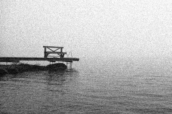
(b) Noisy image

(c) $M=0$

(d) $M=10\text{ (PSNR-optimal)}$

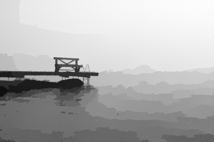
(e) $M=40\text{ (SSIM-optimal)}$

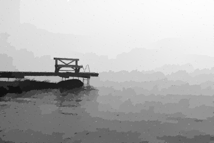
(f) $M=\infty$

Figure 1: Pier photo denoising results with noise level $\sigma=30$ (Gaussian), for varying cut-off $M$, fixed $q=0.4$ and fixed $\alpha^{\infty}=0.0207$.

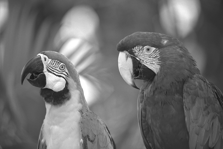
(a) Original

(b) Noisy image

(c) $M=0\text{ (PSNR-optimal)}$

(d) $M=15\text{ (SSIM-optimal)}$

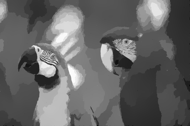
(e) $M=40$

(f) $M=\infty$

Figure 2: Parrot photo denoising results with noise level $\sigma=30$ (Gaussian), for varying cut-off $M$, fixed $q=0.5$ and fixed $\alpha^{\infty}=0.0253$.

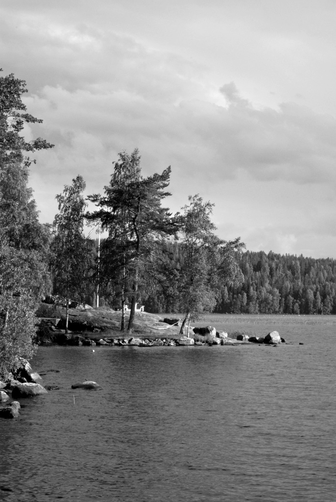
(a) Original

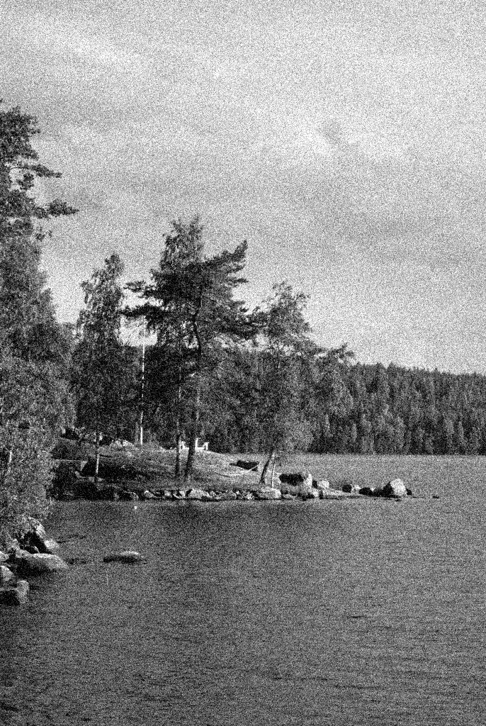
(b) Noisy image

(c) $M=0$

(d) $M=20\text{ (PSNR-optimal)}$

Figure 3: Summer photo denoising results with noise level $\sigma=60$ (Gaussian), for varying cut-off $M$, fixed $q=0.3$ and fixed $\alpha^{\infty}=0.00430$.

Effect of the $\eta$ term

(Another file with old results…)

3.3 Conclusion

Conclusion

We may conclude: • The cut-off $M$ for linearising $t^{q}$ – Is required theoretically – Can be seen in image gradient statistics – Improves results in practise • The multiscale regularisation $\eta$ is a “theoretical artefact” that has yet to be justified in practise.

Thank you for your attention!