A measurement of gravitational lensing of the Cosmic Microwave Background by galaxy clusters using data from the South Pole Telescope

Abstract

Clusters of galaxies are expected to gravitationally lens the cosmic microwave background (CMB) and thereby generate a distinct signal in the CMB on arcminute scales. Measurements of this effect can be used to constrain the masses of galaxy clusters with CMB data alone. Here we present a measurement of lensing of the CMB by galaxy clusters using data from the South Pole Telescope (SPT). We develop a maximum likelihood approach to extract the CMB cluster lensing signal and validate the method on mock data. We quantify the effects on our analysis of several potential sources of systematic error and find that they generally act to reduce the best-fit cluster mass. It is estimated that this bias to lower cluster mass is roughly $0.85\sigma$ in units of the statistical error bar, although this estimate should be viewed as an upper limit. We apply our maximum likelihood technique to 513 clusters selected via their SZ signatures in SPT data, and rule out the null hypothesis of no lensing at $3.1\sigma$. The lensing-derived mass estimate for the full cluster sample is consistent with that inferred from the SZ flux: $M_{200,\mathrm{lens}}=0.83_{-0.37}^{+0.38}\,M_{200,\mathrm{SZ}}$ (68%  C.L., statistical error only).

1. Introduction

Gravitational lensing of the cosmic microwave background (CMB) by large-scale structure (LSS) has recently emerged as a powerful cosmological probe. The first detection of this effect relied on measuring the cross-correlation between CMB lensing maps and radio galaxy counts (Smith et al., 2007). Subsequent studies have correlated CMB lensing maps with several different galaxy populations (e.g., Hirata et al., 2008; Bleem et al., 2012; Planck Collaboration et al., 2014b), quasars (e.g., Hirata et al., 2008; Sherwin et al., 2012; Planck Collaboration et al., 2014b), and maps of the cosmic infrared background (Holder et al., 2013; Planck Collaboration et al., 2014c), to give just a few examples. These measurements of the correlation between CMB lensing and intervening structure have used massive objects as effectively point-like tracers of LSS and have thus been sensitive to the clustering of the dark matter halos these objects inhabit. In the context of the halo model, this clustering signal is the “two-halo term” (for a review of the halo model see Cooray & Sheth, 2002).

The lensing of the CMB due to the galaxies or clusters themselves is sensitive to the structure of the individual halos, i.e., the “one-halo” term. Madhavacheril et al. (2014) have recently reported a measurement of the lensing of the CMB by dark matter halos with masses $M\sim 10^{13}\,{\rm M}_{\odot}$ using CMB data from the Atacama Cosmology Telescope Polarimeter stacked on the locations of roughly 12,000 CMASS galaxies from the SDSS-III/BOSS survey. Galaxy clusters, with halo masses $M\gtrsim 10^{14}\,{\rm M}_{\odot}$, offer another promising target for measuring lensing of the CMB by individual halos.

Seljak & Zaldarriaga (2000) showed that lensing by galaxy clusters induces a dipole-like distortion in the CMB that is proportional to and aligned with the CMB gradient behind the cluster. Consider a galaxy cluster lying along the line of sight to a pure gradient in the CMB. Photon trajectories on either side of the cluster are bent towards the cluster, causing these photons to appear to have originated farther away from the cluster. The net result is that the CMB temperature appears decreased on the hot side of the cluster and increased on the opposite side. In the absence of a CMB temperature gradient behind the cluster, gravitational lensing does not lead to a measurable distortion (this can be seen as a consequence of the fact that gravitational lensing conserves surface brightness). The magnitude of the CMB cluster lensing distortion is therefore sensitive to the mass distribution of the cluster, its redshift, and also the pattern of the CMB on the last scattering surface in the direction of the cluster. For a typical CMB gradient of $13\mu\rm{K}/\rm{arcmin}$ and a cluster with mass $M\sim 10^{15}\,{\rm M}_{\odot}$ located at $z\sim 1$ (a high mass, high redshift cluster), the lensing distortion in the CMB peaks at $\sim 10$$\mu$K  roughly $1$ arcminute from the cluster center.

Current CMB experiments do not have the sensitivity to obtain high significance detections of the lensing effect around single clusters. To detect this effect, then, we must combine the constraints from many clusters to increase the signal-to-noise. Since the lensing distortion induced by a cluster is sensitive to the mass of the cluster, the combined lensing constraint can be translated into a constraint on the weighted average of the cluster masses in the sample. For the time being, CMB lensing constraints on cluster mass are unlikely to be competitive with other means of measuring cluster masses, such as lensing of the light from background galaxies (e.g., Johnston et al., 2007; Okabe et al., 2010; Hoekstra et al., 2012; High et al., 2012; von der Linden et al., 2014). Still, such measurements provide a useful cross-check on other techniques for measuring cluster mass because they are sensitive to different sources of systematic error. Future CMB experiments with higher sensitivity will dramatically improve the signal-to-noise of CMB cluster lensing measurements. If sources of systematic error can be controlled, high signal-to-noise measurements of CMB cluster lensing can provide cosmologically useful cluster mass constraints, especially at $z\gtrsim 1$ (Lewis & King, 2006). Furthermore, if both CMB lensing and galaxy lensing constraints can be obtained on a set of clusters, these measurements can be combined to yield interesting constraints on e.g., dark energy (Hu et al., 2007b).

Several authors have considered the detectability of the effect and how well CMB cluster lensing can constrain cluster masses (e.g., Seljak & Zaldarriaga, 2000; Holder & Kosowsky, 2004; Vale et al., 2004; Dodelson, 2004; Lewis & King, 2006; Lewis & Challinor, 2006). Various approaches to extract the signal have also been investigated: Seljak & Zaldarriaga (2000) and Vale et al. (2004) considered fitting out the gradient in the CMB to extract the cluster signal; Holder & Kosowsky (2004) considered an approach based on Wiener filtering; Lewis & Challinor (2006) and Yoo & Zaldarriaga (2008) developed a maximum likelihood approach; and Hu et al. (2007a) and Melin & Bartlett (2014) considered approaches based on the optimal quadratic estimator of Hu (2001) and Hu & Okamoto (2002). Many of these techniques rely on a separation of scales inherent to the problem: the distortions caused by cluster lensing are a few arcminutes in angular size, while the primordial CMB has little structure on these scales as a result of diffusion damping. This simple picture is complicated by the fact that instrumental noise and foreground emission may lead to arcminute size structure in the observed temperature field. Furthermore, any method to extract the CMB cluster lensing signal must be robust to contamination from the thermal and kinematic Sunyaev-Zel’dovich (SZ) effects (Sunyaev & Zel’dovich, 1972, 1980), as well as other foregrounds.

In this paper we present a $3.1\sigma$ measurement of the arcminute scale gravitational lensing of the CMB by galaxy clusters using data from the full 2500 deg² SPT-SZ survey (e.g., Story et al., 2013). We develop a maximum likelihood approach to extract the CMB cluster lensing signal based on a model for the lensing-induced distortion. Our approach differs somewhat from those mentioned above in that it is inherently parametric: we directly constrain the parameters of an assumed mass profile rather than generating a map of the lensing mass. The method is validated via application to mock data and is then applied to observations of the CMB around 513 clusters identified in the SPT-SZ survey via their SZ effect signature (Bleem et al., 2015). The mass constraints from each cluster are combined to constrain the weighted average of the cluster masses in our sample. As a null test, we also analyze many sets of off-cluster observations and find no significant detection.

The paper is organized as follows: in §2 we describe the data set used in this work and in §3 we develop a maximum likelihood approach to extract the CMB cluster lensing signal from this data set. The results of our analysis applied to mock data and our estimation of systematic effects are presented in §4. The analysis is applied to SPT data in §5, and conclusions are given in §6.

2. Data

2.1. CMB Data

The data used in this work were collected with the South Pole Telescope (SPT, Carlstrom et al., 2011) as part of the SPT-SZ survey. The SPT-SZ survey covered roughly 2500 deg² of the southern sky to an approximate depth of 40, 18, and 80 $\mu$K-arcmin in frequency bands centered at 95, 150, and 220 GHz, respectively. The SPT-SZ maps used in this analysis are identical to those described in George et al. (2014). The maps are projected using the oblique Lambert azimuthal equal-area projection and are divided into square pixels measuring 0.5 arcminutes on a side.

The 2500 deg²  SPT-SZ survey area was subdivided into 19 contiguous fields, each of which was observed to full survey depth before moving on to the next. The fields were observed using a sequence of left-going and right-going scans. Each pair of scans is at a constant elevation, and the elevation is increased in a discrete step between pairs. Denoting left-going and right-going scans as $L$ and $R$, the sky map is the sum $\frac{1}{2}(L+R)$ of maps generated from these two scan directions. The difference map formed via the combination $\frac{1}{2}(L-R)$ should have no sky signal and can be used as a statistically representative estimate of the instrumental and atmospheric noise (henceforth, we will sometimes refer to these two noise sources simply as “instrumental noise,” since the distinction is irrelevant for our purposes). Because the observing strategy varies somewhat between different fields, so does the level of instrumental noise. Below, we will estimate the instrumental noise levels in a field-dependent fashion. More detailed descriptions of the SPT observation strategy may be found in George et al. (2014) and references therein.

Each sky map used in this work is the sum of signal from the sky and instrumental noise. The signal contribution to the maps can be expressed as the convolution of the true sky with an instrumental-plus-analysis response function. The response function characterizes how astrophysical objects would appear in the SPT-SZ maps and consists of two components: a “beam function” that accounts for the SPT beam shape, and a “transfer function” that accounts for the time-stream filtering of the SPT data. As with the instrumental noise, variations in the observation strategy between different fields cause the transfer function of the maps to also vary between fields. The characterizations of the SPT transfer and beam functions are described in George et al. (2014) and references therein. We treat the transfer function in a field-dependent fashion below. In §3 we use the measured beam and transfer functions to fit for the CMB cluster lensing signal in the SPT-SZ data.

2.2. tSZ-free Maps

The Sunyaev-Zel’dovich effect is the distortion of the CMB induced by inverse-Compton scattering of CMB photons and energetic electrons (for a review see Birkinshaw, 1999). This effect is especially pronounced in the directions of massive galaxy clusters as these objects are reservoirs of hot, ionized gas. The SZ effect from clusters can be divided into two parts: the thermal SZ effect (tSZ) and the kinematic SZ effect (kSZ). The tSZ effect is due to inverse-Compton scattering of CMB photons with hot intra-cluster electrons. The effect has a distinct spectral signature that makes a cluster appear as a cold spot in the CMB at low frequencies and a hot spot at high frequencies, with a null at 217 GHz. If the cluster also has a peculiar velocity relative to the CMB rest frame, the CMB will appear anisotropic to the cluster, and an additional Doppler shift will be imprinted on the scattered CMB photons. This distortion, known as the kSZ effect, is frequency independent when expressed as a brightness temperature fluctuation.

The magnitude of the tSZ effect around galaxy clusters can be significantly greater than the magnitude of the CMB cluster lensing signal. A cluster with mass $M\sim 5\times 10^{14}\,{\rm M}_{\odot}$ introduces a tSZ signal of roughly $-400$$\mu$K  (as compared to roughly 5$\mu$K  from lensing) at the cluster center when observed at 150 GHz. Introducing this level of SZ contamination into our mock analysis (see §3.6) biases the lensing mass constraints to such an extreme degree that we lose the ability to measure CMB cluster lensing. Eliminating the tSZ is therefore essential to our analysis.

We exploit the frequency dependence of the tSZ to remove it from our data. Since SPT observes at 95, 150, and 220 GHz, we form a linear combination of the data at these three frequencies that nulls the tSZ effect, but preserves the CMB signal. This tSZ-free linear combination is created as follows. First, all three maps are smoothed to the resolution of the 95 GHz map since that map has the lowest angular resolution ($\sim$1.6 arcmin). Next, a linear combination of the 95 and 150 GHz maps that cancels the tSZ while preserving the primordial CMB is generated. Lastly, this linear combination map is added to the 220 GHz map (which is assumed to be tSZ-free since 220 GHz corresponds roughly to the null in the tSZ) with inverse variance weighting to minimize the noise in the final map. We note that this last step, the combination of the 95/150 GHz linear combination data with the 220 GHz data, could benefit from an optimal weighting of the two data sets as a function of angular multipole. The analysis presented here effectively uses a different, sub-optimal weighting. We also ignore relativistic corrections to the tSZ spectrum (Itoh et al., 1998), which negligibly affect the construction of the tSZ-free linear combination.

The noise level of the resulting tSZ-free map is roughly 55 $\mu$K-arcmin, significantly higher than the 18 $\mu$K-arcmin noise in the 150 GHz data: we have sacrificed statistical sensitivity to remove the tSZ-induced bias. We use only this tSZ-free linear combination in the analysis presented here. Because the kSZ is not frequency dependent, it is not eliminated with this approach; we will return to its effects in §4.3.1.

2.3. Galaxy Cluster Catalog

The galaxy clusters used in this analysis were selected via their tSZ signatures in the 2500 deg² SPT-SZ survey as described in Bleem et al. (2015). We select all clusters with signal-to-noise $\xi>4.5$ and with measured optical redshifts, resulting in 513 clusters. The clusters analyzed in this work have a median redshift of $z=0.55$ and 95% of the clusters lie in the $0.14<z<1.25$ redshift interval. Bleem et al. (2015) derived cluster mass estimates for this sample using a scaling relation between $M_{500}$ and the SZ detection significance. As described there, the calibration of this scaling relationship is somewhat sensitive to the assumed cosmology: adopting the best fit $\Lambda$CDM model from Reichardt et al. (2013) lowers the cluster mass estimates by $8\%$ on average, while adopting the best fit parameters from WMAP9 (Hinshaw et al., 2013) or Planck (Planck Collaboration et al., 2014a) increases the cluster mass estimates by $4\%$ and $17\%$, respectively. For the cosmological parameters adopted in Bleem et al. (2015) (flat $\Lambda$CDM with $\Omega_{m}=0.3$, $h=0.7$, $\sigma_{8}=0.8$), the median SZ-derived mass of the cluster sample is $M_{500}=3.6\times 10^{14}\,{\rm M}_{\odot}$ and 95% of the clusters lie in the range $2.5\times 10^{14}\,{\rm M}_{\odot}<M_{500}<9.6\times 10^{14}\,{\rm M}_{\odot}$. We make use of these mass estimates to generate mock data in §3.6 and in §5 we compare these SZ-derived masses to the cluster masses derived from our measurement of CMB cluster lensing.

2.4. Map Cutouts and the Noise Mask

The lensing analysis presented here is performed on “cutouts” from the tSZ-free maps. Each cutout measures 5.5 arcminutes on a side. These cutouts are centered on the galaxy clusters’ positions determined in Bleem et al. (2015), and we refer to these as “on-cluster” cutouts.

For the purposes of null tests (i.e., confirming that we observe no signal when no CMB cluster lensing is occurring), we have produced many sets of “off-cluster” cutouts centered on random positions in the maps. To ensure that these off-cluster cutouts have noise properties representative of the on-cluster cutouts, we draw these random points from a sub-region of the map that we refer to as the “noise mask”, defined as follows. First, for each field we define the weight map, $w$, which is approximately proportional to the inverse variance of the instrumental noise at each position in the map. Given the weight map of a particular field, we select positions that have weights between $0.95w_{\rm{min}}$ and $1.05w_{\rm{max}}$, where $w_{\rm{min}}$ and $w_{\rm{max}}$ are the minimum and maximum weights at all cluster locations in the field, respectively. Finally, we exclude from the noise mask any portion of the map that is within 10 arcminutes of an identified point source or cluster. The point source catalog used for this purpose is taken from George et al. (2014) and includes all point sources detected at greater than $5\sigma$  ($\sim$6.4 mJy at 150 GHz). For each cluster, we randomly draw 50 off-cluster cutouts from the noise mask region of the field in which the cluster resides. This procedure gives us 50 sets of 513 off-cluster cutouts that have the same noise properties as our 513 on-cluster cutouts. To be robust, our lensing analysis should not detect any cluster lensing on these off-cluster cutouts, and we confirm this fact explicitly below.

3. Analysis

We have developed a maximum likelihood technique for constraining the CMB cluster lensing signal. This approach relies on computing the full pixel-space likelihood of the data given a model for the lensing deflection angles sourced by a cluster. The likelihood function extracts all the information contained in the data about the model parameters.

The unlensed CMB is known to be very close to a Gaussian random field (e.g., Planck Collaboration et al., 2014d). As such, the likelihood of observing a particular set of pixelized temperature values, $\vec{d}$, can be computed given a model for the covariance between these pixels, $\mathbf{C}$. The Gaussian likelihood is:

$$\mathcal{L}(\mathbf{C}|\vec{d})=\frac{1}{\sqrt{(2\pi)^{N_{\mathrm{pix}}}\det\mathbf{C}}}\exp\left[-\frac{1}{2}\vec{d}^{T}\mathbf{C}^{-1}\vec{d}\right],$$ (1)

where $N_{\mathrm{pix}}$ is the number of pixels in $\vec{d}$. Our model for the data includes contributions from three sources:

$$\mathbf{C}=\mathbf{C}_{\mathrm{CMB}}+\mathbf{C}_{\mathrm{foregrounds}}+\mathbf{C}_{\mathrm{noise}},$$ (2)

where $\mathbf{C}_{\mathrm{CMB}}$ is the covariance due to the CMB, $\mathbf{C}_{\mathrm{foregrounds}}$ is the covariance due to signals on the sky that are not CMB, and $\mathbf{C}_{\mathrm{noise}}$ is the covariance due to instrumental noise. In Eq. 1 we have defined the data vector to be the deviation from the mean CMB temperature so that $\langle\vec{d}\rangle=0$.

We model the foreground and noise covariances as Gaussian. The dominant foreground in our measurement is due to the cosmic infrared background (CIB). Although non-Gaussianity is present in the CIB (Crawford et al., 2014; Planck Collaboration et al., 2014e), the level of non-Gaussianity is small. For example, Crawford et al. (2014) measured the bispectrum of the 220 GHz CIB Poisson term to be $B$$\sim$1.7$\times 10^{-10}\mu\rm{K}^{3}$. This contributes approximately $B^{2/3}=3.1\times 10^{-7}\mu\rm{K}^{2}$ to the power spectrum, which is only $\sim$1% of the 220 GHz CIB Poisson power spectrum measured by George et al. (2014), $C=4.6\times 10^{-5}\mu\rm{K}^{2}$.

3.1. The Lensed CMB Covariance Matrix

Gravitational lensing is a surface brightness-preserving remapping of the unlensed CMB. This means that a photon that is observed at direction $\hat{n}$ originated from the direction $\hat{n}_{\mathrm{unlensed}}=\hat{n}+\vec{\delta}(\hat{n})$, where $\vec{\delta}(\hat{n})$ is the gravitational lensing deflection field. Lensing thus changes the covariance structure of $\mathbf{C}_{\mathrm{CMB}}$. Since the cluster position is uncorrelated with the CMB temperature, the mean of the data will remain zero. In principle, $\mathbf{C}_{\mathrm{foregrounds}}$ can also change as a result of gravitational lensing if, for instance, some of the foreground emission is sourced from behind the cluster. This issue warrants careful consideration and we will return to it in more detail below. $\mathbf{C}_{\mathrm{noise}}$ is, of course, unaffected by gravitational lensing since it is not cosmological.

Because we are interested in the behavior of the CMB on small angular scales comparable to the sizes of galaxy clusters, a flat sky approximation is appropriate here and we can replace $\hat{n}$ with the planar $\vec{x}$. The calculation of the lensed CMB covariance matrix, $\mathbf{C}_{\mathrm{CMB}}(M)$, for a cluster of mass $M$ then proceeds exactly as in the unlensed case (e.g., Dodelson, 2003), except $\vec{x}$ must be replaced with $\vec{x}_{\mathrm{unlensed}}=\vec{x}+\vec{\delta}^{M}(\hat{n})$ (the superscript $M$ here is used to indicate that the deflection field is a function of the cluster mass). We find that the elements of the lensed covariance matrix can be written as

$$\mathbf{C}_{\rm{CMB},ij}(M)=$$

$$\int d^{2}x\int d^{2}x^{\prime}\,B_{i}(\vec{x})B_{j}(\vec{x}^{\prime})g(\vec{x}+\vec{\delta}^{M}(\vec{x}),\vec{x}^{\prime}+\vec{\delta}^{M}(\vec{x}^{\prime})),$$

where

$$g(\vec{x}+\vec{\delta}^{M}(\vec{x}),\vec{x}^{\prime}+\vec{\delta}^{M}(\vec{x}^{\prime}))$$

$$\approx \sum_{l}C_{l}\frac{(2l+1)}{4\pi}J_{0}\left(l\left|(\vec{x}+\vec{\delta}^{M}(\vec{x}))-(\vec{x}^{\prime}+\vec{\delta}^{M}(\vec{x}^{\prime}))\right|\right),$$

and $J_{0}$ is the zeroth order Bessel function of the first kind. Here, $B_{i}(\vec{x})$ is the pixelized beam and transfer function for pixel $i$; i.e., given a true sky signal $f(\vec{x})$, a noiseless experiment would measure a signal in pixel $i$ equal to $s_{i}=\int d^{2}xB_{i}(\vec{x})f(\vec{x})$. For ease of notation, we lump the telescope beam and transfer functions into a single object; in reality, these two functions are sourced by very different mechanisms as was discussed in §2. $C_{l}$ is the power spectrum of the CMB, which we obtain from CAMB (Lewis et al., 2000; Howlett et al., 2012) using the best-fit WMAP7+SPT cosmology from Story et al. (2013). Here we use the lensed CMB power spectrum to account for the LSS present at redshifts below and above the cluster redshift.

3.2. The Deflection Angle Template

The lensed CMB covariance matrix can be computed from Eq. 3.1 given a model for the deflection field sourced by the cluster. The deflection field can in turn be computed from a model for the cluster mass distribution if the cluster redshift is known. In this analysis, we assume a Navarro-Frenk-White (NFW) profile for the cluster mass distribution, parameterized in terms of $M_{200}$ and the concentration, $c$ (Navarro et al., 1996). Written in this way, the NFW profile is

$$\rho(r)=\frac{(200/3)c^{3}}{\ln(1+c)-\tfrac{c}{1+c}}\frac{\rho_{\mathrm{crit}}(z)}{\left(\tfrac{rc}{r_{200}}\right)\left(1+\tfrac{rc}{r_{200}}\right)^{2}},$$ (5)

where $\rho(r)$ is the mass density a distance $r$ from the center of the cluster; $\rho_{\mathrm{crit}}(z)=3H^{2}(z)/(8\pi G)$ is the critical density for closure of the Universe at redshift $z$; and $r_{200}$ is defined to be the radius at which the mean enclosed density is $200\rho_{\mathrm{crit}}(z)$. The mass enclosed within this radius is $M_{200}=(800\pi/3)\rho_{\mathrm{crit}}(z)r_{200}^{3}$. Henceforth, when referring to the cluster mass we will use $M_{200}$ rather than the more generic $M$. The concentration parameter, $c$, controls how centrally concentrated the density profile is, with higher values of $c$ resulting in a more centrally peaked mass distribution. Simulations suggest that $c$ is a slowly varying function of the cluster mass and redshift; for a $M_{200}=5\times 10^{14}\,{\rm M}_{\odot}$ cluster, the expected concentration is $c\sim$2.7 (Duffy et al., 2008). Since we are concerned with halos of mass $M_{200}\sim 5\times 10^{14}\,{\rm M}_{\odot}$ here and because our likelihood constraints are only weakly sensitive to the concentration, we fix $c=3$ throughout. The results obtained by varying $c$ from 2 to 5 are essentially identical, as we discuss in §4.3.4.

While the NFW profile is a common choice for parameterizing the density profiles of galaxy clusters, true cluster density profiles may exhibit significant deviations from this form. High resolution dark matter-only simulations, for instance, suggest that the density profiles of the inner cores of clusters are flatter than predicted by the NFW formula (which diverges as $r^{-1}$ for small $r$) (e.g., Merritt et al., 2006; Navarro et al., 2010). The introduction of baryonic effects into such simulations has also been shown to significantly impact the cluster density profile at small $r$, causing departures from the NFW form (e.g., Gnedin et al., 2004; Duffy et al., 2010; Gnedin et al., 2011; Schaller et al., 2014). Simulations also suggest that for massive or rapidly accreting halos, the outer density profile ($r\gtrsim 0.5\,r_{200}$) declines more rapidly than predicted by the NFW formula (e.g., Diemer & Kravtsov, 2014). Finally, halos of galaxy clusters are not expected to be perfectly spherical, but rather triaxial (e.g., Jing & Suto, 2002). Still, despite these caveats, the NFW profile has proven an excellent fit to weak lensing observations of galaxy clusters. Although the density profile of an individual galaxy cluster may exhibit significant deviations from the NFW form, the profile averaged over many clusters – such as the 513 clusters considered here – has been shown to be very well described by an NFW mass distribution (e.g., Johnston et al., 2007; Okabe et al., 2010; Newman et al., 2013). Furthermore, departures from the NFW profile in the central part of the cluster are unlikely to have much effect on our results because of the low resolution (roughly 1 arcminute) of our data, and because the mass of the core is a small fraction of the total cluster mass. Ultimately, the NFW profile is more than adequate for our purposes since the current data set does not have the resolution or sensitivity to distinguish between different profiles. We constrain the potential systematic effects introduced into our analysis by departures from the NFW profile in §4.2.

For a NFW profile, the deflection vector at angular position $\vec{\theta}$ away from the cluster is

$$\vec{\delta}^{M}\left(\theta\right)=-\frac{16\pi GA}{cr_{200}}\frac{\vec{\theta}}{\theta}\frac{d_{\rm{SL}}}{d_{\rm{S}}}f(d_{\rm{L}}\theta c/r_{200}),$$ (6)

where $d_{\rm{L}}$, $d_{\rm{S}}$ and $d_{\rm{SL}}$ are the angular diameter distances to the lens, to the source, and between the source and the lens, respectively, and $\theta=|\vec{\theta}|$ (Bartelmann, 1996; Dodelson, 2004). The function $f(x)$ is given by

$$f(x)=\frac{1}{x}\begin{cases}\ln(x/2)+\frac{\ln\left(x/[1-\sqrt{1-x^{2}}]\right)}{\sqrt{1-x^{2}}},&\text{if}\ x<1\\ \ln(x/2)+\frac{\pi/2-\arcsin(1/x)}{\sqrt{x^{2}-1}},&\text{if}\ x>1\end{cases}$$ (7)

and the constant $A$ is related to $M_{200}$ and $c$ via

$$A=\frac{M_{200}c^{2}}{4\pi\left[\ln(1+c)-c/(1+c)\right]}.$$ (8)

In our analysis we allow the cluster mass to be negative; a negative cluster mass simply means that the deflection vector is pointed in the opposite direction of that predicted for a positive cluster mass of equal magnitude.

3.3. Numerical Implementation

With the measured beam and transfer functions of SPT and the deflection angle template of Eq. 6, the predicted $\mathbf{C}_{\mathrm{CMB}}(M_{200})$ can be computed by direct integration of Eq. 3.1. Unfortunately, evaluating the 4D integral in Eq. 3.1 is computationally expensive and the full covariance matrix must be computed many times. Consequently, we instead rely on Monte Carlo simulations to calculate the lensed CMB covariance matrix.

The unlensed covariance matrix is first computed at 1.0 arcminute resolution across an angular window 70.5 arcminutes on a side (this wide range relative to the cluster cutouts – which are only 5.5 arcminute on a side – ensures that we capture the full effects of the SPT beam and transfer function). In the absence of lensing, Eq. 3.1 can be simplified significantly, and the unlensed covariance elements can be quickly calculated (e.g., Dodelson, 2003). Many Gaussian realizations of this unlensed covariance matrix (i.e., realizations of the unlensed CMB) are then generated. Next, a high resolution (0.1 arcminute) map of the deflection field is generated for a particular $M_{200}$ and $z$. The unlensed CMB maps are then interpolated at the positions of the deflected high-resolution pixels. Since the primordial CMB is smooth on scales below a few arcminutes this interpolation is very accurate. The resultant maps are then degraded to the resolution of the tabulated beam and transfer functions, which are applied to the mock maps using Fast Fourier Transforms. Finally, the mean of the product of the lensed temperatures in pairs of pixels, $d_{i}d_{j}$, is computed across the many simulated realizations of the lensed CMB. This mean serves as our estimate of ${\bf C}_{\mathrm{CMB}}(M_{200})$.

Our baseline analysis uses 20,000 simulated realizations of the lensed CMB to form an estimate of the lensed CMB covariance matrix. To ensure that this procedure has reached the precision required for our analysis, we repeat the covariance estimation using fewer and lower-resolution simulations. We find that decreasing the number of simulations by a factor of two, increasing the pixel size at which the lensing operation is performed by a factor of 2.5, and decreasing the window size from 70.5 arcmin to 60.5 arcmin all lead to small changes in the estimated covariances matrices (on the order of a few percent). We also repeat the full likelihood analysis using the degraded covariance estimates and find that the change in the likelihood is entirely negligible (less than a percent in most cases). We are therefore confident that our covariance estimation procedure has acheived sufficient precision for the analysis presented here.

Even when performed in the Monte Carlo fashion described above, the computation of the lensed CMB covariance matrix is still computationally expensive. To speed up the analysis of the data even more, we compute the lensed covariance matrix across a grid of $M_{200}$ and $z$; the lensed covariance matrix at the desired mass and redshift can then be computed via interpolation. Our baseline analysis uses 31 evenly spaced $M_{200}$ values and 7 evenly spaced $z$ values. To determine whether the accuracy of the covariance interpolation is sufficient for our measurement, we have increased the resolution of the $M_{200}$ and $z$ grid across which the covariance matrix is evaluated and have found the impact on our likelihood results to be negligible.

3.4. Noise and Foreground Covariance

To compute the likelihood in Eq. 1 we must also estimate $\mathbf{C}_{\mathrm{nf}}\equiv\mathbf{C}_{\mathrm{noise}}+\mathbf{C}_{\mathrm{foregrounds}}$. We take the approach of computing this combination of covariances directly from the data. Since the noise level varies somewhat from field to field, the estimation of $\mathbf{C}_{\mathrm{nf}}$ must be performed separately for each field. To do this, we randomly sample cutouts from the SPT maps of each field to measure the covariance of the observed data, $\mathbf{C}_{\mathrm{obs}}$. These samples are drawn from the noise mask region defined in §2.4. $\mathbf{C}_{\mathrm{nf}}$ is then estimated by subtracting the predicted CMB-only covariance from the measured CMB+noise+foreground covariance, i.e., $\mathbf{C}_{\mathrm{nf}}=\mathbf{C}_{\mathrm{obs}}-\mathbf{C}_{\mathrm{CMB}}(M_{200}=0)$.

If the foregrounds are lensed by the cluster it is possible for $\mathbf{C}_{\mathrm{foregrounds}}$ to vary with $M_{200}$. Modeling foreground lensing, however, would require knowledge of the redshift distribution of the foregrounds; for the sake of simplicity we assume that the foregrounds remain unlensed in our analysis. We quantify the bias introduced into our analysis by this assumption using mock data, as described in §4.2. For the purposes of generating this mock data, it is useful to have estimates of both $\mathbf{C}_{\mathrm{noise}}$ and $\mathbf{C}_{\mathrm{foregrounds}}$ (rather than only the sum $\mathbf{C}_{\mathrm{noise}}+\mathbf{C}_{\mathrm{foregrounds}}$). To estimate $\mathbf{C}_{\mathrm{noise}}$ we sample cutouts from the $L-R$ difference maps described in §2.1. This sampling procedure is done using the same noise masks as above so that $\mathbf{C}_{\mathrm{noise}}$ accurately reflects the noise at the cluster locations.

$\mathbf{C}_{\mathrm{foregrounds}}$, on the other hand, is estimated using previous constraints on the power spectra of the dominant foreground sources. For the tSZ-free maps that we use in this analysis, the dominant foregrounds are the ‘Poisson’ and ‘clustered’ components constrained in Reichardt et al. (2012). The Poisson foreground results from point sources below the detection threshold that are randomly distributed on the sky and has $C_{l}=C_{0}$, independent of $l$. The amplitude of the Poisson component is estimated from the data. The clustered foreground model accounts for the clustering of point sources and is modeled as $D_{l}\equiv C_{l}l(l+1)/(2\pi)=D_{0}$ independent of $l$ for $l<1500$, and $D_{l}\propto l^{0.8}$ for $l>1500$. The amplitude of the clustered component is taken from Reichardt et al. (2012), adjusted to account for the fact that our maps are constructed from a weighted combination of observations at three frequencies. With the foreground power spectra determined, $\mathbf{C}_{\mathrm{foregrounds}}$ can be calculated in the same way as the unlensed CMB covariance matrix.

We emphasize that the main analysis estimates $\mathbf{C}_{\mathrm{nf}}\equiv\mathbf{C}_{\mathrm{noise}}+\mathbf{C}_{\mathrm{foregrounds}}$ directly from the data, and that the individual estimates of $\mathbf{C}_{\mathrm{noise}}$ and $\mathbf{C}_{\mathrm{foregrounds}}$ are used only to test for certain systematic effects using mock data.

3.5. Combining the Likelihoods

With our estimates of $\mathbf{C}_{\mathrm{CMB}}(M_{200})$ and $\mathbf{C}_{\mathrm{noise}}+\mathbf{C}_{\mathrm{foregrounds}}$, we now have all the ingredients necessary to evaluate the likelihood in Eq. 1. For a cutout around the $i$th cluster, we evaluate the likelihood, $\mathcal{L}_{i}(M_{200})$, as a function of $M_{200}$ to constrain the effects of CMB lensing by that cluster. However, since the instrumental noise is large relative to the CMB cluster lensing signal, we do not expect to obtain a detection of the lensing effect around a single cluster. Instead, we must combine constraints from multiple clusters. One way to accomplish this is to compute the likelihood $\mathcal{L}_{\mathrm{total}}(M_{200})=\prod_{i}^{N_{\mathrm{clusters}}}\mathcal{L}_{i}(M_{200})$, where $N_{\mathrm{clusters}}=513$ is the number of clusters in our sample. This method of combining likelihoods is appealing because it is simple and because it depends only on the lensing information.

Not all the masses in the sample are the same, so the above treatment – which assumes all clusters share a common mass – provides more of an estimate of the detection significance than any useful information on the masses of the clusters in the sample. Furthermore, the spread in masses will likely lead to a spread in the width of the likelihood function, i.e., a degradation in the signal-to-noise. Some of this can be recaptured by scaling the $M_{200}$ parameter for each cluster by an external mass estimator for that cluster, and indeed estimates of each cluster’s mass can be obtained from the strength of the SZ signal at the cluster location. Here we use the SZ-determined cluster masses from Bleem et al. (2015) that were discussed in §2.3. We convert the $M_{500,\mathrm{SZ}}$ measured in Bleem et al. (2015) into $M_{200,\mathrm{SZ}}$ using the Duffy et al. (2008) mass-concentration relation. So an improved likelihood that includes this information is written not as a function of $M_{200}$, but rather as

$$\mathcal{L}_{i}\rightarrow\mathcal{L}_{i}\left(\frac{M_{200}}{M_{200,\mathrm{SZ}}}\,M_{200,\mathrm{SZ},i}\right),$$ (9)

with a new free global parameter $M_{200}/M_{200,\mathrm{SZ}}$. The individual cluster likelihoods expressed as functions of $M_{200}/M_{200,\mathrm{SZ}}$ can then be combined as before:

$$\mathcal{L}_{\mathrm{total}}\left(\frac{M_{200}}{M_{200,\mathrm{SZ}}}\right)=\prod_{i}^{N_{\mathrm{clusters}}}\mathcal{L}_{i}\left(\frac{M_{200}}{M_{200,\mathrm{SZ}}}\,M_{200,\mathrm{SZ},i}\right).$$

Note, however, that any intrinsic scatter in the relationship between the lensing-derived $M_{200}$ and the SZ-derived $M_{200,\mathrm{SZ}}$ will lead to additional broadening of the combined multi-cluster likelihood as a function of $M_{200}/M_{200,\mathrm{SZ}}$. We will employ both methods of combining individual cluster likelihoods in §5.

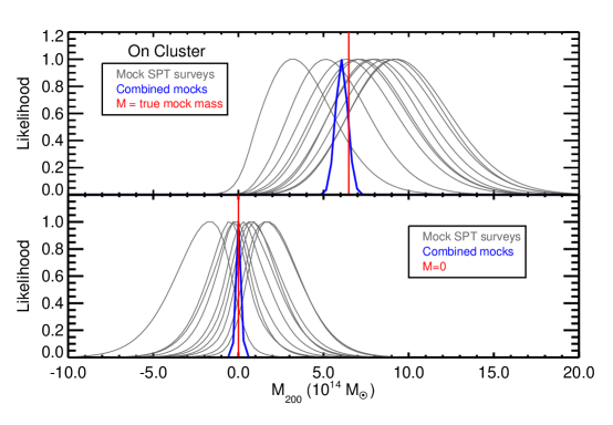
Figure 1.— Constraints on $M_{200}$ from the analysis of mock data that is designed to mimic real data from the SPT. The top panel shows the likelihood as a function of $M_{200}$ for patches centered on clusters; the bottom panel shows the same for patches centered at random points (off-cluster). Each gray curve represents the constraint obtained from a single realizations of an SPT-like survey that detects 513 clusters; the blue curves are combined constraints from 50 such realizations.

3.6. Mock Data

In order to test our analysis pipeline and study possible sources of systematic error we generate and analyze mock data. The mock data sets include contributions from the lensed (and unlensed) CMB, foregrounds and noise. The mock cluster redshift distribution is identical to the redshift distribution of the real clusters. To generate cluster masses for our mock catalog, we convert the SZ-derived $M_{500}$ values described in §2.3 to $M_{200}$ assuming that the clusters are described by NFW profiles with the Duffy et al. (2008) mass-concentration relation. The resultant sample has a median mass of $M_{200}=5.6\times 10^{14}\,{\rm M}_{\odot}$ and 95% of the clusters have $4.0\times 10^{14}\,{\rm M}_{\odot}<M_{200}<1.37\times 10^{15}\,{\rm M}_{\odot}$.

For each mock cluster, a realization of the lensed and unlensed CMB was generated in the same manner described in §3.3. The clusters were distributed among the SPT fields identically to the real clusters, and the appropriate beam and transfer functions for each field were applied. Gaussian realizations of the measured noise and foreground covariance matrix, $\mathbf{C}_{\mathrm{nf}}$, were added to the mock data in a field-dependent fashion. The process of generating a mock cluster catalog was repeated 50 times to build statistics. Each mock catalog includes entirely new realizations of the CMB, foregrounds and noise.

4. Results on Mock Catalogs

4.1. Projections

The results of our analysis of the mock cluster cutouts are shown in Fig. 1. The top panel shows the results of analyzing the mock data when CMB lensing is turned on, while the bottom panel shows the results when CMB lensing is turned off (i.e., a null test). Each gray curve represents the combined likelihood constraints from an SPT-like survey with 513 clusters generated in the manner described above; the blue curves show the combined constraints from 50 mock data sets of 513 clusters. The vertical red line in the top panel indicates the true mean cluster mass in the mock survey. Each mock data set strongly prefers a positive cluster mass over $M_{200}\leq 0$. The combined constraint from 50 mock data sets in Fig. 1 illustrates that the likelihood prefers the mean cluster mass of the sample. When the analysis is performed on the unlensed mock data (bottom panel), none of the 50 mock data sets yield a significant detection, and the mean is centered at the (correct) value of $M_{200}=0$.

To quantify the significance of our measurement of CMB cluster lensing (for both mock and real data) we use a likelihood ratio test. Since we are interested in whether or not the data prefer lensing over the null hypothesis of no lensing (i.e., $M_{200}=0$), we define the likelihood ratio

$$\Lambda=\frac{\mathcal{L}(M_{200}=0)}{\max\mathcal{L}(M_{200})}.$$ (11)

In the large sample size limit (i.e., many clusters), $-2\ln\Lambda$ should be $\chi^{2}(k=1)$-distributed with $k=1$ degree of freedom. Note that this statement does not assume that the likelihood for each cluster is Gaussian as a function of $M_{200}$. The $p$-value for the measurement is then found by integrating the $\chi^{2}(k=1)$ distribution below $-2\ln\Lambda$. Our reported detection significance is calculated by converting this $p$-value into a standard, two-sided Gaussian significance and is exactly equal to $\sqrt{-2\ln\Lambda}$. All detection significances are reported in this way below. Averaging across the 50 mocks discussed above, we find that the mean detection significance for an SPT-like survey (i.e., 513 mock clusters) is $3.4\sigma$.

4.2. Systematics Tests

Several sources of systematic error can potentially affect our CMB cluster lensing measurement. We quantify the impact of these systematic effects on our analysis by modeling them in mock data. For the purposes of these systematic tests we generate new mock data consisting of 500 realizations of the CMB, noise, and foregrounds for a single cluster with $z=0.55$ and $M_{200}=5.6\times 10^{14}\,{\rm M}_{\odot}$, corresponding to the median redshift and SZ-derived mass for clusters in our sample. Various systematic effects are introduced to this mock data set as described below. We then analyze the mock data neglecting the presence of the systematic effects and measure how the likelihood changes.

We express the bias introduced by each systematic as the fractional shift in the maximum likelihood mass: $(M^{\rm{ML}}_{\rm{sys}}-M^{\rm{ML}})/M^{\rm{true}}$, where $M^{\rm{ML}}_{\rm{sys}}$ is the maximum likelihood mass in the presence of the systematic, $M^{\rm{ML}}$ is the maximum likelihood mass without the systematic, and $M^{\rm{true}}=5.6\times 10^{14}\,{\rm M}_{\odot}$ is the true mass of the mock clusters. This process is repeated 50 times and we report the mean value of the bias across these trials. We caution that this procedure is not meant to rigorously quantify the systematic error budget of our lensing constraints; we have, after all, assumed a single mass and redshift for all of the mock clusters. Instead, these estimates are provided for two purposes. First, they suggest that the individual systematic errors associated with our cluster mass measurement are likely small compared to the statistical error bars on this measurement. Second, the estimates provided below highlight the relative importance of each of the systematic effects that we consider here.

4.2.1 Monopole Contamination

The first systematic that we consider is anything that leads to a signal at the cluster center (a “monopole”). The CMB cluster lensing signal vanishes at the cluster center and therefore has no monopole component. Since our model includes no other signals correlated with the cluster, any residual monopole-like signal at the cluster location is not included in our model and could therefore bias our analysis. One important potential source of monopole contamination is residual tSZ in our tSZ-free maps. Although the linear combination map used is nominally independent of tSZ, the finite width of the observing bands and relativistic corrections to the tSZ (Itoh et al., 1998) can produce a small residual component. Other potential sources of monopole contamination include the integrated dusty emission or radio emission from cluster member galaxies much too faint to be individually detected in SPT maps. Strong emission from individual cluster members is treated in the next section.

We determine the amplitude of such contamination directly from our data. Stacking all of the cluster cutouts reveals that the level of monopole contamination is consistent with a $\beta$ profile (Cavaliere & Fusco-Femiano, 1976, 1978) with $\beta=1$, $\theta_{c}=0.5$ arcmin, and an amplitude of $-3$ $\mu$K  for each cluster. We introduce this level of contamination into our 50 sets of 500 mock cutouts and repeat the likelihood analysis (just as before, without accounting for the monopole contamination) to determine how our likelihood constraints are affected. Across 50 sets of mock cutouts, we find that monopole contamination of the measured amplitude leads to a shift in the maximum likelihood mass that is $\lesssim 1\%$, well below the statistical precision of our cluster mass constraint.

4.3. Emission from Individual Cluster Members

The contamination of our measurement by a single bright cluster galaxy does not in general behave like the monopole contamination considered above. In particular, a single source could fill in one side of the cluster lensing dipole if its projected position relative to the cluster is at a particular radius and orientation. At 150 GHz and a resolution of 1.6 arcmin, a 1 mJy source will have an equivalent CMB fluctuation temperature of $10$$\mu$K  and, assuming a spectral index of $\alpha=-0.5$, will have a temperature fluctuation of roughly $-$10$\mu$K  in our tSZ-free maps. We simulate the effects of such sources on our analysis by introducing a single point source with beam-smoothed amplitude of $-$10$\mu$K  into each of our mock cutouts. We choose the location of the point source randomly across a disk of radius 1.5 arcmin centered on the cluster. Since the CMB cluster lensing dipole is expected to peak at  $\sim$1 arcmin away from the cluster center, sources located much farther than this should have little effect on our measurement.

We find that introducing this level of point source contamination into our mock data causes the inferred cluster mass to be biased low by  $\sim$7% on average across our 50 sets of 500 mock cluster cutouts. In reality, however, not every cluster is expected to have an associated point source of this magnitude and proximity to the cluster. Using the De Zotti et al. (2010) model for radio source counts at 150 GHz and the results of Coble et al. (2007), we estimate that only  $\sim$5% of SPT-SZ clusters will have a 1 mJy or greater source within 1.5 arcmin of the cluster center. We only consider radio sources in this calculation because models of dusty sources predict fewer bright sources (e.g., Negrello et al., 2007), and because star formation is suppressed in cluster environments (e.g., Bai et al., 2007). The resulting bias on the mean mass of our cluster sample would thus be  $<$1%, well below our statistical precision.

4.3.1 kSZ

The second systematic that we consider is the kSZ effect. The kSZ effect results from scattering of CMB photons with electrons that have bulk velocities relative to the Hubble flow. Motions of cluster electrons could be due, for instance, to the cluster falling towards nearby superstructures or because the cluster is rotating. While typically much smaller than the tSZ effect, the kSZ effect is frequency independent when expressed as a change in brightness temperature, so the tSZ-free linear combination map contains a kSZ component.

The diffuse kSZ caused by linear or quasi-linear structure will act only as a source of noise in this analysis, and, because its amplitude is much smaller than the instrumental noise (George et al., 2014), it can be safely ignored here. Instead we turn our attention to the kSZ due to the galaxy clusters themselves. This cluster kSZ signal will have two components: a component due to the bulk motion of the cluster, and a component due to internal velocities.

To include the effects of the bulk component of the kSZ in our mock data we rely on the work of Sehgal et al. (2010), which used $N$-body simulations and models for the gas physics at different redshifts to generate maps of the kSZ effect. The Sehgal et al. (2010) kSZ maps are generated by assigning a single velocity to all gas associated with each cluster, and thus provide an estimate of the kSZ signal due to the bulk velocity of each cluster. The simulated kSZ signal is introduced into our mock cutouts by extracting cutouts from the Sehgal et al. (2010) kSZ maps around clusters with $M_{200}$ between $5.0\times 10^{14}\,{\rm M}_{\odot}$ and $6.0\times 10^{14}\,{\rm M}_{\odot}$. This selection ensures that the kSZ signal is reasonably well matched to our mock clusters, which have masses of $5.6\times 10^{14}\,{\rm M}_{\odot}$. The likelihood analysis of the mock cutouts with kSZ is then performed as before, ignoring the presence of the kSZ.

Across 50 realizations of the mock data, the introduction of a bulk-velocity kSZ component causes the maximum likelihood mass to be biased low by $9\%$ on average, below the statistical precision of this work. We note that our analysis of mock data with kSZ suggests that the size of the bias introduced by the presence of the kSZ depends on the level of instrumental noise and foregrounds in the data. If the foreground or instrumental noise contributions are very small, the bias introduced by the kSZ can become significant. Future experiments with higher sensitivity may need to take a more careful approach to accounting for the kSZ.

The mock kSZ signal considered above does not include the effects of a kSZ signal due to internal motions of gas within the cluster. Of particular concern is the kSZ signal resulting from cluster rotation, which we call rkSZ. A cluster that is rotating will induce a dipole-like kSZ signal since one side of the cluster will be moving towards us while the other will be moving away. Consequently, even though the rkSZ is expected to be small, it is a potentially serious contaminant for the CMB cluster lensing measurement because of its similar morphology on the sky. Unlike the CMB cluster lensing signal, though, the rkSZ dipole is not preferentially aligned with the gradient of the CMB temperature field.

Our model for the rkSZ signal is based on the model of Chluba & Mannheim (2002), where it is assumed that a galaxy cluster rotates as a solid body, motivated in part by the work of Bullock et al. (2001) and Cooray & Chen (2002). Modeling the electron number density as a $\beta$-profile, Chluba & Mannheim (2002) derive an expression for the rkSZ signal:

$$\frac{\Delta T_{\mathrm{rkSZ}}}{T_{\mathrm{CMB}}}(\theta,\phi) = A_{{\rm rkSZ}}\theta\sin i\sin\phi\left(1+\frac{\theta^{2}}{\theta_{\mathrm{core}}^{2}}\right)^{1/2-3\beta/2},$$

where $A_{{\rm rkSZ}}$ is a parameter that controls the amplitude of the signal, $\theta$ is the angular distance from the cluster center, $\phi$ is the transverse angular coordinate and $i$ is the inclination angle of the cluster. We set $\beta=1$ and $\theta_{\mathrm{core}}=1$ arcminute as these values are fairly typical for the clusters in our sample.

The amplitude of the rkSZ signal, $A_{{\rm rkSZ}}$, is not very well constrained at present. Simulations (e.g., Nagai et al., 2003; Fang et al., 2009; Bianconi et al., 2013) suggest that the rotational velocities of clusters are typically small compared to the cluster velocity dispersion. However, in clusters that have recently experienced mergers, the rotational velocities may be significantly larger. Chluba & Mannheim (2002) argue that typical peak rkSZ signals are in the range $0.1$–10$\mu$K, but could be as high as 100$\mu$K  for a recent merger.

The model rkSZ signal is introduced into our 50 sets of 500 mock cutouts assuming a constant value of $A_{{\rm rkSZ}}$ for all mock clusters. Each cluster’s inclination angle and orientation on the sky are chosen randomly, however, so the mock rkSZ signal varies from cluster to cluster. We explore several values of $A_{{\rm rkSZ}}$, chosen such that the maximum amplitude of the rkSZ signal (i.e., for an optimally aligned cluster) varies between 1$\mu$K  and 20$\mu$K. We find that the presence of rkSZ in the mock data acts to reduce our measured signal. At a maximum amplitude of 1$\mu$K  the rkSZ introduces a mass bias of less than $1\%$ to our mass constraints, at 5$\mu$K  the peak of the likelihood is biased to lower masses by roughly $8\%$, at 10$\mu$K  the bias is roughly $28\%$ and at 20$\mu$K  the bias is $93\%$. Therefore, it appears that as long as the rkSZ signal is $\lesssim$10$\mu$K , the bias introduced into our mass constraints by such a signal is less than the statistical precision of this work. Since most clusters are expected to have rkSZ signals less than 10$\mu$K, we do not attempt to correct for this effect here. Although clusters that have experienced recent mergers may have rkSZ signals that are higher than 10$\mu$K, the number of such clusters in our sample is likely small.

4.3.2 Foreground Lensing

As discussed above, the degree to which foreground emission is lensed by the cluster is not very well constrained. The CIB – which constitutes the dominant source of foreground emission – is thought to originate from redshifts $z\sim 0.5\textrm{ to }4$. Since our cluster sample is drawn from $0.05\lesssim z\lesssim 1.5$, the amount by which the foregrounds are lensed will likely vary from cluster to cluster. Our analysis, however, assumes that foregrounds remain unlensed. To investigate the effects of this assumption on our analysis, we generate mock cutouts with lensed foregrounds assuming that foreground emission originates from $z=4$. Since the CIB is known to originate from $z\lesssim 4$, setting $z=4$ gives an approximate upper bound to the effects of gravitational lensing on the foregrounds, and therefore an upper limit to the systematic error introduced into our analysis by assuming no foreground lensing.

Realizations of the lensed clustered foreground can be generated using the procedure described in §3.6. Lensing the Poisson foreground is more difficult as this foreground has power extending to arbitrarily small scales, including scales below that at which we generate map realizations. To get around this, we calculate the lensed Poisson covariance matrix directly from the integral in Eq. 3.1 and use this covariance matrix to generate realizations of the lensed Poisson foreground. The mock cutouts with lensed foregrounds are then analyzed as before, assuming that both foregrounds remain unlensed.

Across the 50 sets of 500 mock clusters that we have generated, we find that lensing of the foregrounds causes our $M_{200}$ constraint to be biased low. Lensing of the Poisson foreground contributes the dominant part of this bias, owing to its large contribution to the total covariance relative to that of the clustered foreground. The average mass bias introduced into our mock analysis by lensing of the foregrounds is $7\%$. We do not correct for this bias, as doing so would require a detailed modeling of the redshift distribution of the CIB. We emphasize, though, that the bias measured here is necessarily an overestimate of the true bias introduced by foreground lensing because we have placed the foregrounds at $z=4$ when the true foreground emission results from $z\leq 4$.

4.3.3 Cluster Miscentering

The cluster centers used in our analysis are derived from SPT measurements of the cluster SZ signal and will generally differ from the centers of mass of the clusters. A similar miscentering problem arises in the context of galaxy shear measurements, where the cluster center is typically defined as the location of the brightest cluster galaxy (BCG), even though the BCG may not correspond to the true center of mass of the cluster (e.g., von der Linden et al., 2014). In that context, cluster miscentering can be a significant source of systematic error in cluster mass measurements, causing the masses of miscentered clusters to be underestimated.

We model the effects of imperfect knowledge of the cluster center by applying random positional shifts to our mock cluster data. These offsets are drawn from a two dimensional Gaussian with $\sigma=30$ arcseconds. In this model, 68% of the offsets are smaller than 45 arcseconds. As a point of reference, Song et al. (2012) found that 68% of the offsets between SPT-estimated centers and BCGs were smaller than 38 arcseconds, so the miscentering error introduced here is likely an overestimate. Analyzing the miscentered mock data reveals that the peak likelihood is biased to lower mass by roughly $6\%$ on average, below the statistical precision of our lensing mass constraint. Accurately modeling the size of the miscentering systematic error would require an understanding of how the miscentering error varies with cluster mass and redshift, and we do not attempt such a detailed analysis here.

4.3.4 Uncertainty in the Cluster Mass Profile

Our analysis assumes a NFW profile for each cluster with concentration $c=3$. In reality, the halo concentration is known to vary with cluster mass and redshift, and to exhibit significant scatter. To explore the effects on our analysis of changing the halo concentration, we regenerate the mock cluster data using halos of concentration $c=2.5$ and $c=5$. These two values of the concentration should bracket the expected range of concentrations allowed for the clusters in our sample, including effects of uncertainty in the assumed cosmological parameters (Dutton & Macciò, 2014). The data are then analyzed as before, assuming $c=3$. We find that changing the concentration has an essentially negligible effect on our analysis, which is not surprising given that our constraints are not sensitive enough to distinguish between slightly different behaviors of the inner mass profile. Across 50 realizations of 513 mock clusters, we find that the maximum likelihood mass increases on average by less than 1% when $c=5$, well below the statistical precision of our measurements. When $c=2.5$ we find that the maximum likelihod mass decreases by about 1$\%$. The effects of changing halo concentration can therefore be safely ignored in this analysis.

A related source of potential bias is halo triaxiality. It is well known from simulations (e.g. Jing & Suto, 2002; Kasun & Evrard, 2005) that halo density profiles are not perfectly spherical. Deviations from sphericity could introduce a bias into our analysis because we have assumed a perfectly spherical NFW profile. Corless & King (2007) have found that in the context of traditional galaxy shear measurements, fitting a spherical NFW profile to the extreme case of a halo elongated along the line of sight can lead to a 50% mass bias. Averaged over all possible halo orientations, however, Corless & King (2007) find that the mean recovered mass is very close to the true mass. Given the low sensitivity of our mass constraints and the findings of Corless & King (2007), it is unlikely that halo triaxiality has a significant impact on our results. A detailed modeling of the effects of halo triaxiality is beyond the scope of this work.

Finally, we consider deviations of the halo profile from the NFW form itself. While large deviations from the NFW profile are expected in the central region of the dark matter halo, the roughly 1.6 arcminute resolution of the SZ-free maps means that we are not very sensitive to the behavior of the density profile in this regime. Deviations from the NFW form are also expected for massive clusters in the outskirts of the halo, $r\gtrsim 0.5r_{200}$ (Diemer & Kravtsov, 2014). Assuming the SZ-derived masses described in §2.3, the median $\theta_{200}=r_{200}/d_{A}(z)$ for the clusters in our sample is 5.2 arcminutes, where $d_{A}(z)$ is the angular diameter distance to the cluster. This means that our angular window of 5.5 arcminutes around each cluster is probing $r\sim 0.5r_{200}$. Consequently, deviations from the NFW form in the $r\gtrsim 0.5r_{200}$ regime could potentially introduce a systematic error into our mass constraints.

We model the effects of deviations from the NFW density profile by approximating the results of Diemer & Kravtsov (2014). Mock data with a non-NFW deflection profile are generated and analyzed assuming the usual NFW deflection formula. We find that modifying the form of the deflection profile in this way biases the best fit mass low by roughly $10\%$ on average across our 50 sets of 500 mock cluster cutouts.

4.3.5 Large Scale Structure

Our NFW lensing template (Eq. 6) accounts only for deflections of CMB photons caused by the cluster itself. It therefore ignores deflections that could be caused by the presence of LSS near the line of sight to the cluster. Lensing by LSS unassociated with the cluster changes the covariance properties of the CMB in a well-known way (e.g. Seljak, 1996). This effect is approximated in our model through the use of the LSS-lensed $C_{l}$’s in computing the model covariance matrix (Eq. 3.1). However, it is well known that clusters live in overdense environments. Lensing induced by LSS that is associated with the cluster is not included in our model and could therefore bias our analysis.

In the language of the halo model, we have effectively ignored the two-halo contribution to the lensing signal. However, weak lensing data (e.g. Johnston et al., 2007) suggest that within a few virial radii of the cluster center, the one-halo term dominates the lensing signal. Since the analysis presented here considers a small angular region around each cluster that extends to only $\leq 1$ virial radius, it is safe to neglect the two-halo term in this analysis.

4.3.6 Cluster Selection

One remaining potential systematic is related to the SZ-selection method. The SPT clusters have been selected at the locations of decrements in the 95 and 150 GHz maps. Simulations show that clusters selected in this fashion will preferentially sit on decrements in the CMB, and this effect could potentially bias the mass inferred from CMB lensing. However, the bias in the background CMB is small, on the order of -1$\mu$K, and the resulting effect on the CMB lensing mass is likely to be small compared to our statistical error.

4.3.7 Combined Systematic Effects

The above discussion has considered how several different systematic effects can individually bias our lensing constraints. We now attempt to estimate the total bias resulting from the combination of multiple systematic effects. Our combined systematic model includes the five most significant biases considered above. We include the bulk motion kSZ, the rkSZ with peak amplitude of 5$\mu$K, and foreground lensing as described in §4.3.2. The clusters are miscentered as described in §4.3.3 and the cluster density profile used is the Diemer & Kravtsov (2014) profile described in §4.3.4. We find that the mean bias introduced by this combined systematic model is a 39% bias to lower cluster mass. The measured bias is consistent with the product of the individual biases (34%), given the scatter among the 50 simulation realizations. A 39% bias to lower cluster mass amounts to a roughly $0.85\sigma$ shift in units of the statistical uncertainty. This should be interpreted as an approximate upper limit on the bias to lower cluster mass, as we have placed all of the foreground emission at $z=4$ and have likely over-estimated the effect of miscentering. We do not attempt to correct for this systematic bias, although doing so would not alter the main conclusions of this work, as discussed in Section 6.

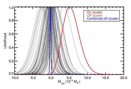
Figure 2.— Constraints on $M_{200}$ resulting from analysis of SPT data. The thick red curve is our result for 513 on-cluster cutouts, while each thin gray curve is our result for a separate realization of 513 off-cluster cutouts. The combined constraint from the 50 sets of off-cluster cutouts is the thick blue curve.

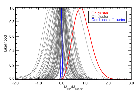
Figure 3.— Same as Fig. 2 except the likelihood has been computed as a function of $M_{200}/M_{200,\mathrm{SZ}}$, where $M_{200,\mathrm{SZ}}$ is the cluster mass computed from the measured tSZ signal as described in Bleem et al. (2015).

5. Results

Fig. 2 shows the results of our likelihood analysis applied to the data described in §2. The red curve represents our constraint from the analysis of 513 on-cluster cutouts. Each of the 50 gray curves represents the constraint from 513 off-cluster cutouts chosen from the same fields as the on-cluster cutouts in the manner described in §2. The thick blue curve is the combined constraint from the 50 sets of off-cluster cutouts.

The on-cluster likelihood in Fig. 2 shows a preference for positive mass. We find that $M_{200}=0$ is ruled out at $3.1\sigma$ using the likelihood ratio test described above. We assume a flat prior on $M_{200}$ so that the posterior probability of $M_{200}$ is directly proportional to the likelihood. Integrating the posterior on $M_{200}$ yields a 68% confidence band of $M_{200}=5.1_{-2.1}^{+2.5}\times 10^{14}\,{\rm M}_{\odot}$. The results of our analysis of the SPT clusters are also consistent with the projections from mock data, which had a mean detection significance of 3.4$\sigma$. The off-cluster likelihoods shown in Fig. 2 (gray curves) are consistent with $M_{200}=0$. The worst null likelihood has a detection significance of $2.2\sigma$, which is reasonable since we have considered 50 null likelihoods. The combined constraint from all 50 null likelihoods is also consistent with $M_{200}=0$ at $0.84\sigma_{\rm 50}$, where $\sigma_{50}$ is the standard deviation computed from the 50 stacked likelihoods. There is therefore no evidence of any bias in our off-cluster analysis.

As described in §3.5, the constraints on the lensing mass $M_{200}$ of our cluster sample can be translated into constraints on the ratio between the lensing mass, $M_{200,\mathrm{lens}}$, and the cluster mass estimated from the tSZ effect, $M_{200,\mathrm{SZ}}$. The likelihood curve of the ratio $M_{200,\mathrm{lens}}/M_{200,\mathrm{SZ}}$ is calculated per cluster, and the combined constraint (assuming a flat prior on the ratio) is

$$\frac{M_{200,\mathrm{lens}}}{M_{200,\mathrm{SZ}}}=0.83_{-0.37}^{+0.38}\qquad({\rm 68\%}\,C.L.)$$ (13)

The mean mass inferred from CMB cluster lensing is consistent with the mean mass inferred from the tSZ signal at $0.5\sigma$. This constraint and the corresponding off-cluster likelihoods are shown in Fig. 3. Using the likelihood ratio test described above, we find that $M_{200,\mathrm{lens}}/M_{200,\mathrm{SZ}}=0$ is ruled out at $3.1\sigma$.

As pointed out in §2.3, depending on the assumed cosmological model, the mean SZ-derived cluster mass can vary by as much as $17\%$. Our constraint on $M_{200,\mathrm{lens}}/M_{200,\mathrm{SZ}}$ should therefore be viewed in the context of the cosmological model assumed in Bleem et al. (2015), from which our SZ-derived cluster masses are taken. Additionally, intrinsic scatter in the relationship between $M_{200,\mathrm{SZ}}$ and $M_{200,\mathrm{lens}}$ will lead to broadening of the likelihood as a function of $M_{200,\mathrm{lens}}/M_{200,\mathrm{SZ}}$. However, the expected level of intrinsic scatter between the true cluster mass and $M_{200,\mathrm{SZ}}$ is only  $\sim$15% per cluster (Benson et al., 2013). Given our $3.1\sigma$ detection significance across all clusters, the per-cluster constraint on the lensing mass is roughly  $\sqrt{513}/3.1\sim 730\%$. The effect of intrinsic scatter in the SZ-derived masses is therefore only $1-730/\sqrt{730^{2}+15^{2}}\sim 0.02\%$, and is therefore negligible here.

6. Conclusions

We have presented a measurement of CMB cluster lensing using data from the SPT. Our data rule out the null hypothesis (that cluster lensing is not occurring) at $3.1\sigma$ and constrain the weighted average cluster mass of our sample to be $M_{200}=5.1_{-2.1}^{+2.5}\times 10^{14}\,{\rm M}_{\odot}$ (68% confidence limit). Our cluster mass constraint – obtained by measurement of the CMB cluster lensing effect – is less precise than other cluster mass estimates, but it does offer a confirmation of SZ-derived mass estimates with completely independent sources of systematic errors: ${M_{200,\mathrm{lens}}}/{M_{200,\mathrm{SZ}}}=0.83_{-0.37}^{+0.38}$ (68%  C.L.). Our lensing mass constraint is consistent with ${M_{200,\mathrm{lens}}}/{M_{200,\mathrm{SZ}}}=1$ at $0.5\sigma$.

We have investigated several potential sources of systematic error and have found that their individual effects are significantly less than the statistical uncertainties of our mass constraints. We find that the most important systematic effects are the bulk velocity kSZ, the kSZ due to a rotating cluster, lensing of foregrounds by the clusters, cluster miscentering and deviation of the cluster density profile from the NFW form in the outskirts of the cluster. These findings are in agreement with other investigations into CMB cluster lensing systematic effects (e.g. Holder & Kosowsky, 2004; Lewis & King, 2006), although the contaminating effects of foreground lensing appear to be underappreciated in the literature.

All of the five most important systematic effects listed above bias our lensing constraint to lower masses. In our mock analysis, the presence of these five systematic effects results in an average bias of 39% to lower cluster mass. This level of bias amounts to roughly $0.85\sigma$ in units of the statistical error bar. We emphasize, though, there are several uncertainties involved in the calculation of this bias. For one, we have almost certainly overestimated the effects of foreground lensing on our analysis by placing all foreground emission at $z=4$. Furthermore, our estimate of the bias caused by cluster miscentering is likely an overestimate as well because of our simplified treatment of this effect. Finally, the amplitude of the rotating-cluster kSZ signal is poorly constrained at present, and its effects on our analysis are therefore somewhat uncertain. Because of the large uncertainties associated with our estimates of systematic effects, we have chosen to not include corrections for these effects in our reported detection significance, and instead compute the detection significance from the statistical error bar alone.

Correcting for the measured 39% bias to lower cluster mass would cause the likelihood to prefer higher cluster mass and would therefore yield a higher detection significance as well as a higher ${M_{200,\mathrm{lens}}}/{M_{200,\mathrm{SZ}}}$. If the same bias is assumed for each cluster, a 39% shift to higher cluster mass would cause the best fit ${M_{200,\mathrm{lens}}}/{M_{200,\mathrm{SZ}}}$ to increase to roughly 1.15, still consistent with ${M_{200,\mathrm{lens}}}/{M_{200,\mathrm{SZ}}}=1$ to within the error bars. There is therefore no evidence from this analysis of tension with the SZ-derived cluster masses, even accounting for potentially large systematic biases.

Additionally, as discussed in §5, systematic uncertainty on $M_{200,\mathrm{SZ}}$ may affect our constraint on ${M_{200,\mathrm{lens}}}/{M_{200,\mathrm{SZ}}}$. In particular, the SZ-derived masses used in this work could potentially be overestimated by as much as 8% or underestimated by as much as 17%, depending on the assumed cosmological parameters. Our constraint on ${M_{200,\mathrm{lens}}}/{M_{200,\mathrm{SZ}}}$ is derived assuming the same cosmological parameters used in Bleem et al. (2015) and should be considered in that context. Even if the maximal bias is assumed for the SZ-derived cluster masses, our analysis does not yield tension with ${M_{200,\mathrm{lens}}}/{M_{200,\mathrm{SZ}}}=1$ at greater than $1\sigma$. This statement remains true even if the lensing-derived masses are increased by 38% to account for the systematic biases discussed above.

Upcoming data sets offer the exciting possibility of significantly improved measurements of CMB cluster lensing. The measurement presented here using data from the SPT-SZ survey is noise limited: the lensing signal is at the few $\mu$K  level and is on few arcminute scales, while the noise in the tSZ-free linear combination is roughly 55 $\mu$K-arcmin. Ongoing experiments such as SPTpol (Austermann et al., 2012) and ACTPol (Naess et al., 2014), and future experiments such as SPT-3G (Benson et al., 2014), Advanced ACTPol (Calabrese et al., 2014), the Simons Array (Arnold et al., 2014), and so-called Stage IV CMB experiments (e.g., Abazajian et al., 2015) will have significantly lower noise levels than the SPT-SZ survey, allowing them to obtain significantly stronger detections of the CMB cluster lensing signal. Furthermore, these experiments will include additional information about lensing in the form of polarization data. In the primordial CMB, the odd-parity (B-mode) component of the CMB polarization field is expected to be uncorrelated with both the temperature field and the even-parity (E-mode) component of the polarization field. Consequently, lensing induced correlations between B modes and either temperature modes or E modes can be used as a relatively clean probe of CMB lensing (e.g., Hu & Okamoto, 2002). Furthermore, polarization offers another handle on eliminating contamination from the SZ effect. The polarized SZ effect (both thermal and kinematic) from clusters is expected to be significantly smaller (i.e., less than 10-100 nK, Carlstrom et al. 2002) than the unpolarized effect, so polarization observations should offer a less-contaminated window into CMB cluster lensing (e.g., Holder & Kosowsky, 2004).

With higher sensitivity data than that employed here, CMB cluster lensing has the potential to provide powerful constraints on cluster masses. In principle, these mass constraints can be used to improve cluster mass-observable relationships that are essential for using clusters as cosmological probes. However, our analysis of potential contaminating effects in §4.2 suggests that there is still much work to be done in reducing systematic errors associated with measurements of CMB cluster lensing. Particularly important are contamination from the kSZ effect, lensing of foregrounds, and departure from the NFW profile at large radii. In principle, both the kSZ and lensing of the foregrounds can be modeled and incorporated into the analysis to eliminate any bias that these effects introduce. However, uncertainty on the amplitude of the kSZ and uncertainty on the foreground redshift distribution limits our ability to accurately perform this modeling at present.

References

- Abazajian et al. (2015) Abazajian, K. N., Arnold, K., Austermann, J., et al. 2015, Astroparticle Physics, 63, 66
- Arnold et al. (2014) Arnold, K., Stebor, N., Ade, P. A. R., et al. 2014, in Society of Photo-Optical Instrumentation Engineers (SPIE) Conference Series, Vol. 9153, Society of Photo-Optical Instrumentation Engineers (SPIE) Conference Series, 1
- Austermann et al. (2012) Austermann, J. E., Aird, K. A., Beall, J. A., et al. 2012, in Society of Photo-Optical Instrumentation Engineers (SPIE) Conference Series, Vol. 8452, Society of Photo-Optical Instrumentation Engineers (SPIE) Conference Series
- Bai et al. (2007) Bai, L., Marcillac, D., Rieke, G. H., et al. 2007, ApJ, 664, 181
- Bartelmann (1996) Bartelmann, M. 1996, A&A, 313, 697
- Benson et al. (2013) Benson, B. A., de Haan, T., Dudley, J. P., et al. 2013, ApJ, 763, 147
- Benson et al. (2014) Benson, B. A., Ade, P. A. R., Ahmed, Z., et al. 2014, in Society of Photo-Optical Instrumentation Engineers (SPIE) Conference Series, Vol. 9153, Society of Photo-Optical Instrumentation Engineers (SPIE) Conference Series
- Bianconi et al. (2013) Bianconi, M., Ettori, S., & Nipoti, C. 2013, MNRAS, 434, 1565
- Birkinshaw (1999) Birkinshaw, M. 1999, Phys. Rep., 310, 97
- Bleem et al. (2012) Bleem, L. E., van Engelen, A., Holder, G. P., et al. 2012, ApJ, 753, L9
- Bleem et al. (2015) Bleem, L. E., Stalder, B., de Haan, T., et al. 2015, ApJS, 216, 27
- Bullock et al. (2001) Bullock, J. S., Dekel, A., Kolatt, T. S., et al. 2001, ApJ, 555, 240
- Calabrese et al. (2014) Calabrese, E., Hložek, R., Battaglia, N., et al. 2014, JCAP, 8, 10
- Carlstrom et al. (2002) Carlstrom, J. E., Holder, G. P., & Reese, E. D. 2002, ARA&A, 40, 643
- Carlstrom et al. (2011) Carlstrom, J. E., Ade, P. A. R., Aird, K. A., et al. 2011, PASP, 123, 568
- Cavaliere & Fusco-Femiano (1976) Cavaliere, A., & Fusco-Femiano, R. 1976, A&A, 49, 137
- Cavaliere & Fusco-Femiano (1978) Cavaliere, A., & Fusco-Femiano, R. 1978, A&A, 70, 677
- Chluba & Mannheim (2002) Chluba, J., & Mannheim, K. 2002, A&A, 396, 419
- Coble et al. (2007) Coble, K., Bonamente, M., Carlstrom, J. E., et al. 2007, AJ, 134, 897
- Cooray & Chen (2002) Cooray, A., & Chen, X. 2002, ApJ, 573, 43
- Cooray & Sheth (2002) Cooray, A., & Sheth, R. 2002, Phys. Rep., 372, 1
- Corless & King (2007) Corless, V. L., & King, L. J. 2007, MNRAS, 380, 149
- Crawford et al. (2014) Crawford, T. M., Schaffer, K. K., Bhattacharya, S., et al. 2014, ApJ, 784, 143
- De Zotti et al. (2010) De Zotti, G., Massardi, M., Negrello, M., & Wall, J. 2010, A&A Rev., 18, 1
- Diemer & Kravtsov (2014) Diemer, B., & Kravtsov, A. V. 2014, ApJ, 789, 1
- Dodelson (2003) Dodelson, S. 2003, Modern Cosmology (Academic Press)
- Dodelson (2004) —. 2004, Phys. Rev. D, 70, 023009
- Duffy et al. (2008) Duffy, A. R., Schaye, J., Kay, S. T., & Dalla Vecchia, C. 2008, MNRAS, 390, L64
- Duffy et al. (2010) Duffy, A. R., Schaye, J., Kay, S. T., et al. 2010, MNRAS, 405, 2161
- Dutton & Macciò (2014) Dutton, A. A., & Macciò, A. V. 2014, MNRAS, 441, 3359
- Fang et al. (2009) Fang, T., Humphrey, P., & Buote, D. 2009, ApJ, 691, 1648
- George et al. (2014) George, E. M., Reichardt, C. L., Aird, K. A., et al. 2014, ArXiv e-prints
- Gnedin et al. (2011) Gnedin, O. Y., Ceverino, D., Gnedin, N. Y., et al. 2011, ArXiv e-prints
- Gnedin et al. (2004) Gnedin, O. Y., Kravtsov, A. V., Klypin, A. A., & Nagai, D. 2004, ApJ, 616, 16
- High et al. (2012) High, F. W., Hoekstra, H., Leethochawalit, N., et al. 2012, ApJ, 758, 68
- Hinshaw et al. (2013) Hinshaw, G., Larson, D., Komatsu, E., et al. 2013, ApJS, 208, 19
- Hirata et al. (2008) Hirata, C. M., Ho, S., Padmanabhan, N., Seljak, U., & Bahcall, N. A. 2008, Phys. Rev. D, 78, 043520
- Hoekstra et al. (2012) Hoekstra, H., Mahdavi, A., Babul, A., & Bildfell, C. 2012, MNRAS, 427, 1298
- Holder & Kosowsky (2004) Holder, G., & Kosowsky, A. 2004, ApJ, 616, 8
- Holder et al. (2013) Holder, G. P., Viero, M. P., Zahn, O., et al. 2013, ApJ, 771, L16
- Howlett et al. (2012) Howlett, C., Lewis, A., Hall, A., & Challinor, A. 2012, JCAP, 1204, 027
- Hu (2001) Hu, W. 2001, ApJ, 557, L79
- Hu et al. (2007a) Hu, W., DeDeo, S., & Vale, C. 2007a, New Journal of Physics, 9, 441
- Hu et al. (2007b) Hu, W., Holz, D. E., & Vale, C. 2007b, Phys. Rev. D, 76, 127301
- Hu & Okamoto (2002) Hu, W., & Okamoto, T. 2002, ApJ, 574, 566
- Itoh et al. (1998) Itoh, N., Kohyama, Y., & Nozawa, S. 1998, ApJ, 502, 7
- Jing & Suto (2002) Jing, Y. P., & Suto, Y. 2002, ApJ, 574, 538
- Johnston et al. (2007) Johnston, D. E., Sheldon, E. S., Wechsler, R. H., et al. 2007, ArXiv e-prints
- Kasun & Evrard (2005) Kasun, S. F., & Evrard, A. E. 2005, ApJ, 629, 781
- Lewis & Challinor (2006) Lewis, A., & Challinor, A. 2006, Phys. Rep., 429, 1
- Lewis et al. (2000) Lewis, A., Challinor, A., & Lasenby, A. 2000, Astrophys. J., 538, 473
- Lewis & King (2006) Lewis, A., & King, L. 2006, Phys. Rev. D, 73, 063006
- Madhavacheril et al. (2014) Madhavacheril, M., Sehgal, N., Allison, R., et al. 2014, ArXiv e-prints
- Melin & Bartlett (2014) Melin, J.-B., & Bartlett, J. G. 2014, ArXiv e-prints
- Merritt et al. (2006) Merritt, D., Graham, A. W., Moore, B., Diemand, J., & Terzić, B. 2006, AJ, 132, 2685
- Naess et al. (2014) Naess, S., Hasselfield, M., McMahon, J., et al. 2014, JCAP , 10, 7
- Nagai et al. (2003) Nagai, D., Kravtsov, A. V., & Kosowsky, A. 2003, ApJ, 587, 524
- Navarro et al. (1996) Navarro, J. F., Frenk, C. S., & White, S. D. M. 1996, ApJ, 462, 563
- Navarro et al. (2010) Navarro, J. F., Ludlow, A., Springel, V., et al. 2010, MNRAS, 402, 21
- Negrello et al. (2007) Negrello, M., Perrotta, F., González-Nuevo, J., et al. 2007, MNRAS, 377, 1557
- Newman et al. (2013) Newman, A. B., Treu, T., Ellis, R. S., et al. 2013, ApJ, 765, 24
- Okabe et al. (2010) Okabe, N., Takada, M., Umetsu, K., Futamase, T., & Smith, G. P. 2010, PASJ, 62, 811
- Planck Collaboration et al. (2014a) Planck Collaboration, Ade, P. A. R., Aghanim, N., et al. 2014a, A&A, 571, A16
- Planck Collaboration et al. (2014b) —. 2014b, A&A, 571, A17
- Planck Collaboration et al. (2014c) —. 2014c, A&A, 571, A18
- Planck Collaboration et al. (2014d) —. 2014d, A&A, 571, A24
- Planck Collaboration et al. (2014e) —. 2014e, A&A, 571, A30
- Reichardt et al. (2012) Reichardt, C. L., Shaw, L., Zahn, O., et al. 2012, ApJ, 755, 70
- Reichardt et al. (2013) Reichardt, C. L., Stalder, B., Bleem, L. E., et al. 2013, ApJ, 763, 127
- Schaller et al. (2014) Schaller, M., Frenk, C. S., Bower, R. G., et al. 2014, ArXiv e-prints
- Sehgal et al. (2010) Sehgal, N., Bode, P., Das, S., et al. 2010, ApJ, 709, 920
- Seljak (1996) Seljak, U. 1996, ApJ, 463, 1