Some simple but challenging Markov processes

Abstract

In this note, we present few examples of Piecewise Deterministic Markov Processes and their long time behavior. They share two important features: they are related to concrete models (in biology, networks, chemistry,…) and they are mathematically rich. Their mathematical study relies on coupling method, spectral decomposition, PDE technics, functional inequalities. We also relate these simple examples to recent and open problems.

1 Introduction

A Piecewise deterministic Markov processes (PDMP) is a stochastic process involving deterministic motion punctuated by random jumps. This large class of non diffusion stochastic models was introduced in the literature by Davis [20, 21] (see also [34]). As it will be stressed below, these processes arise naturally in many application areas: biology, communication networks, reliability of complex systems for example. From a mathematical point of view, they are simple to define but their study may require a broad spectrum of tools as stochastic coupling, functional inequalities, spectral analysis, dynamical systems, partial differential equations.

The aim of the present paper is to present simple examples of PDMP appearing in different applied frameworks and to investigate their long time behavior. Rather than using generic technics (as Meyn-Tweedie-Foster-Lyapunov…strategy) we will focus on as explicit as possible estimates. Several open and motivating questions (stability criteria, regularity of the invariant measure(s), explicit rate of convergence…) are also listed along the paper.

Roughly speaking the dynamics of a PDMP on a set $E$ depends on three local characteristics, namely, a flow $\varphi$, a jump rate $\lambda$ and a transition kernel $Q$. Starting from $x$, the motion of the process follows the flow $t\mapsto\varphi_{t}(x)$ until the first jump time $T_{1}$ which occurs in a Poisson-like fashion with rate $\lambda(x)$. More precisely, the distribution of the first jump time is given by

$$\mathbb{P}_{x}(T_{1}>t)=\exp{{\left(-\int_{0}^{t}\!\lambda(\varphi_{s}(x))\,ds\right)}}.$$

Then, the location of the process at the jump time $T_{1}$ is selected by the transition measure $Q(\varphi_{T_{1}}(x),\cdot)$ and the motion restarts from this new point as before. This motion is summed up by the infinitesimal generator:

$$Lf(x)=F(x)\cdot\nabla f(x)+\lambda(x)\int_{E}\!(f(y)-f(x))\,Q(x,dy),$$ (1)

where $F$ is the vector field associated to the flow $\varphi$. In several examples, the process may jump when it hits the boundary of $E$. The boundary of the space $\partial E$ can be seen as a region where the jump rate is infinite (see for example [18] for the study of billiards in a general domain with random reflections).

In the sequel, we denote by $\mathcal{P}(\mathbb{R}^{d})$ the set of probability measures on $(\mathbb{R}^{d},\mathcal{B}(\mathbb{R}^{d}))$ and, for any $p\geqslant 1$, by $\mathcal{P}_{p}(\mathbb{R}^{d})$ the set of probability measures on $(\mathbb{R}^{d},\mathcal{B}(\mathbb{R}^{d}))$ with a finite $p^{th}$-moment: $\mu\in\mathcal{P}_{p}(\mathbb{R}^{d})$ if

$$\int_{\mathbb{R}^{d}}\!\!{{\left|x\right|}}^{p}\,\mu(dx)<+\infty.$$

The total variation distance on $\mathcal{P}(\mathbb{R}^{d})$ is given by

$${{\left\|\nu-\tilde{\nu}\right\|}}_{\mathrm{TV}} =\inf{{\left\{\mathbb{P}(X\neq\tilde{X})\,:\,X\sim\nu,\,\tilde{X}\sim\tilde{\nu}\right\}}}$$

$$=\sup{{\left\{\int\!f\,d\nu-\int\!f\,d\tilde{\nu}\,:\,f\text{ bounded by }1/2\right\}}}.$$

If $\nu$ and $\tilde{\nu}$ are absolutely continuous with respect to $\mu$ with density functions $g$ and $\tilde{g}$, then

$${{\left\|\nu-\tilde{\nu}\right\|}}_{\mathrm{TV}}=\frac{1}{2}\int_{\mathbb{R}^{d}}\!\!{{\left|g-\tilde{g}\right|}}\,d\mu.$$

For $p\geqslant 1$, the Wasserstein distance of order $p$, defined on $\mathcal{P}_{p}(\mathbb{R}^{d})$, is given by

$$W_{p}(\nu,\tilde{\nu})=\inf{{\left\{{{\left[\mathbb{E}{{\left({{\left|X-\tilde{X}\right|}}^{p}\right)}}\right]}}^{1/p}\,:\,X\sim\nu,\,\tilde{X}\sim\tilde{\nu}\right\}}}.$$

Similarly to the total variation distance, the Wasserstein distance of order $1$ has a nice dual formulation:

$$W_{1}(\nu,\tilde{\nu})=\sup{{\left\{\int\!f\,d\nu-\int\!f\,d\tilde{\nu}\,:\,f\text{ is $1$-Lipschitz}\right\}}}.$$

A generic dual expression can be formulated for $W_{p}$ (see [62]).

2 Storage models, with a bandit…

Let us consider the PDMP driven by the following infinitesimal generator:

$$Lf(x)=-\beta xf^{\prime}(x)+\alpha\int_{0}^{\infty}\!(f(x+y)-f(x))\,e^{-y}dy.$$

Such processes appear in the modeling of storage problems or pharmacokinetics that describe the evolution of the concentration of a chemical product in the human body. The present example is studied in [59, 6]. More realistic models are studied in [11, 14]. Similar processes can also be used as stochastic gene expression models (see [42, 65]).

In words, the current stock $X_{t}$ decreases exponentially at rate $\beta$, and increases at random exponential times by a random (exponentially distributed) amount. Let us introduce a Poisson process ${(N_{t})}_{t\geqslant 0}$ with intensity $\alpha$ and jump times ${(T_{i})}_{i\geqslant 0}$ (with $T_{0}=0$) and a sequence ${(E_{i})}_{i\geqslant 1}$ of independent random variables with an exponential law of parameter $1$ independent of ${(N_{t})}_{t\geqslant 0}$. The process ${(X_{t})}_{t\geqslant 0}$ starting from $x\geqslant 0$ can be constructed as follows: for any $i\geqslant 0$,

$$X_{t}=\begin{cases}e^{-\beta(t-T_{i})}X_{T_{i}}&\text{if }T_{i}\leqslant t<T_{i+1},\\ e^{-\beta(T_{i+1}-T_{i})}X_{T_{i}}+E_{i+1}&\text{if }t=T_{i+1}.\end{cases}$$

This model is sufficiently naïve to express the Laplace transform of $X$.

Lemma 2.1 (Laplace transform).

For any $t\geqslant 0$ and $s<1$, the Laplace transform of $X_{t}$ is given by

$$L(t,s):=\mathbb{E}{{\left(e^{sX_{t}}\right)}}=L(0,se^{-\beta t}){{\left(\frac{1-se^{-\beta t}}{1-s}\right)}}^{\alpha/\beta},$$

where $L(0,\cdot)$ stands for the Laplace transform of $X_{0}$. In particular, the invariant distribution of $X$ is the Gamma distribution with density

$$x\mapsto\frac{x^{{\alpha/\beta}-1}e^{-x}}{\Gamma(\alpha/\beta)}\mathds{1}_{[0,+\infty)}(x).$$

Proof.

Applying the infinitesimal generator to $x\mapsto e^{sx}$, one deduces that the function $L$ is solution of the following partial differential equation:

$$\partial_{t}L(t,s)=-\beta s\partial_{s}L(t,s)+\frac{\alpha s}{1-s}L(t,s).$$

More generally, if the random income is non longer exponentially distributed but has a Laplace transform $L_{i}$ then $L$ is solution of

$$\partial_{t}L(t,s)=-\beta s\partial_{s}L(t,s)+\alpha(L_{i}(s)-1)L(t,s).$$

As a consequence, if $G$ is given by $G(t,s)=\log L(t,s)+(\alpha/\beta)\log(1-s)$ then

$$\partial_{t}G(t,s)=-\beta s\partial_{s}G(t,s).$$

The solution of this partial differential equation is given by $G(t,s)=G(0,se^{-\beta t})$. ∎

The next step is to investigate the convergence to equilibrium.

Theorem 2.2 (Convergence to equilibrium).

Let us denote by $\nu P_{t}$ the law of $X_{t}$ if $X_{0}$ is distributed according to $\nu$. For any $x,y\geqslant 0$ and $t\geqslant 0$ and $p\geqslant 1$,

$$W_{p}(\delta_{x}P_{t},\delta_{y}P_{t})\leqslant{{\left|x-y\right|}}e^{-\beta t},$$

and (when $\alpha\neq\beta$)

$${{\left\|\delta_{x}P_{t}-\delta_{y}P_{t}\right\|}}_{\mathrm{TV}}\leqslant e^{-\alpha t}+{{\left|x-y\right|}}\alpha\frac{e^{-\beta t}-e^{-\alpha t}}{\alpha-\beta}.$$ (2)

Moreover, if $\mu$ is the invariant measure of the process $X$, we have for any probability measure $\nu$ with a finite first moment and $t\geqslant 0$,

$${{\left\|\nu P_{t}-\mu\right\|}}_{\mathrm{TV}}\leqslant{{\left\|\nu-\mu\right\|}}_{\mathrm{TV}}e^{-\alpha t}+W_{1}(\nu,\mu)\alpha\frac{e^{-\beta t}-e^{-\alpha t}}{\alpha-\beta}.$$

Remark 2.3 (Limit case).

In the case $\alpha=\beta$, the upper bound (2) becomes

$${{\left\|\delta_{x}P_{t}-\delta_{y}P_{t}\right\|}}_{\mathrm{TV}}\leqslant(1+{{\left|x-y\right|}}\alpha t)e^{-\alpha t}.$$

Remark 2.4 (Optimality).

Applying $L$ to the test function $f(x)=x^{n}$ allows us to compute recursively the moments of $X_{t}$. In particular,

$$\mathbb{E}_{x}(X_{t})=\frac{\alpha}{\beta}+{{\left(x-\frac{\alpha}{\beta}\right)}}e^{-\beta t}.$$

This relation ensures that the rate of convergence for the Wasserstein distance is sharp. Moreover, the coupling for the total variation distance requires at least one jump. As a consequence, the exponential rate of convergence is greater than $\alpha$. Thus, Equation (2) provides the optimal rate of convergence $\alpha\wedge\beta$.

Proof of Theorem 2.2.

Firstly, consider two processes $X$ and $Y$ starting respectively at $x$ and $y$ and driven by the same randomness (i.e. Poisson process and jumps). Then the distance between $X_{t}$ and $Y_{t}$ is deterministic:

$$X_{t}-Y_{t}=(x-y)e^{-\beta t}.$$

Obviously, for any $p\geqslant 1$ and $t\geqslant 0$,

$$W_{p}(\delta_{x}P_{t},\delta_{y}P_{t})\leqslant|x-y|e^{-\beta t}.$$

Let us now construct explicitly a coupling at time $t$ to get the upper bound (2) for the total variation distance. The jump times of ${(X_{t})}_{t\geqslant 0}$ and ${(Y_{t})}_{t\geqslant 0}$ are the ones of a Poisson process ${(N_{t})}_{t\geqslant 0}$ with intensity $\alpha$ and jump times ${(T_{i})}_{i\geqslant 0}$. Let us now construct the jump heights ${(E^{X}_{i})}_{1\leqslant i\leqslant N_{t}}$ and ${(E^{Y}_{i})}_{1\leqslant i\leqslant N_{t}}$ of $X$ and $Y$ until time $t$. If $N_{t}=0$, no jump occurs. If $N_{t}\geqslant 1$, we choose $E^{X}_{i}=E^{Y}_{i}$ for $1\leqslant i\leqslant N_{t}-1$ and $E^{X}_{N_{t}}$ and $E^{Y}_{N_{t}}$ in order to maximise the probability

$$\mathbb{P}{{\left(X_{T_{N_{t}}}+E^{X}_{N_{t}}=Y_{T_{N_{t}}}+E^{Y}_{N_{t}}\big{|}X_{T_{N_{t}}},Y_{T_{N_{t}}}\right)}}.$$

This maximal probability of coupling is equal to

$$\exp{{\left(-|X_{T_{N_{t}}}-Y_{T_{N_{t}}}|\right)}}=\exp{{\left(-|x-y|e^{-\beta T_{N_{t}}}\right)}}\geqslant 1-|x-y|e^{-\beta T_{N_{t}}}.$$

As a consequence, we get that

$${{\left\|\delta_{x}P_{t}-\delta_{y}P_{t}\right\|}}_{\mathrm{TV}} \leqslant 1-\mathbb{E}{{\left[{{\left(1-|x-y|e^{-\beta T_{N_{t}}}\right)}}\mathds{1}_{{\left\{N_{t}\geqslant 1\right\}}}\right]}}$$

$$\leqslant e^{-\alpha t}+|x-y|\mathbb{E}{{\left(e^{-\beta T_{N_{t}}}\mathds{1}_{{\left\{N_{t}\geqslant 1\right\}}}\right)}}.$$

The law of $T_{n}$ conditionally on the event ${{\left\{N_{t}=n\right\}}}$ has the density

$$u\mapsto n\frac{u^{n-1}}{t^{n}}\mathds{1}_{[0,t]}(u).$$

This ensures that

$$\mathbb{E}{{\left(e^{-\beta T_{N_{t}}}\mathds{1}_{{\left\{N_{t}\geqslant 1\right\}}}\right)}}=\int_{0}^{1}\!e^{-\beta tv}\mathbb{E}{{\left(N_{t}v^{N_{t}-1}\right)}}\,dv.$$

Since the law of $N_{t}$ is the Poisson distribution with parameter $\alpha t$, one has

$$\mathbb{E}{{\left(N_{t}v^{N_{t}-1}\right)}}=\alpha te^{\alpha t(v-1)}.$$

This ensures that

$$\mathbb{E}{{\left(e^{-\beta N_{t}}\mathds{1}_{{\left\{N_{t}\geqslant 1\right\}}}\right)}}=\alpha\frac{e^{-\beta t}-e^{-\alpha t}}{\alpha-\beta},$$

which completes the proof. Finally, to get the last estimate, we proceed as follows: if $N_{t}$ is equal to 0, a coupling in total variation of the initial measures is done, otherwise, we use the coupling above. ∎

Remark 2.5 (Another example).

Surprisingly, a process of the same type appears in [37] in the study of the so-called bandit algorithm. The authors have to investigate the long time behavior of the process driven by

$$Lf(y)=(1-p-py)f^{\prime}(y)+qy\frac{f(y+g)-f(y)}{g},$$

where $0<q<p<1$ and $g>0$. This can be done following the lines of the proof of Theorem 2.2.

3 The TCP model with constant jump rate

This section is devoted to the process on $[0,+\infty)$ driven by the following infinitesimal generator

$$Lf(x)=f^{\prime}(x)+\lambda(f(x/2)-f(x))\quad(x\geqslant 0).$$

In other words, the process grows linearly between jump times that are the one of a homogeneous Poisson process with parameter $\lambda$ and it is divided by 2 at these instants of time. See Section 3.4 for concrete motivations and generalizations.

3.1 Spectral decomposition

Without loss of generality, we choose $\lambda=1$ in this section. The generator $L$ of the naïve TCP process preserves the degree of polynomials. As a consequence, for any $n\in\mathbb{N}$, the eigenvalue $\lambda_{n}=-(1-2^{-n})$ is associated to a polynomials $P_{n}$ with degree $n$. As an example,

$$P_{0}(x)=1,\quad P_{1}(x)=x-2\quad\text{and}\quad P_{2}(x)=x^{2}-8x+32/3.$$

Moreover, one can explicitly compute the moments of the invariant measure $\mu$ (see [39]): for any $n\in\mathbb{N}$

$$\int\!x^{n}\,\mu(dx)=\frac{n!}{\prod_{k=1}^{n}(1-2^{-k})}.$$

Roughly speaking, this relation comes from the fact that the functions $m_{n}:t\in[0,\infty)\mapsto\mathbb{E}(X_{t}^{n})$ for $n\geqslant 0$ are solution of

$$m_{n}^{\prime}(t)=nm_{n-1}(t)+{{\left(2^{-n}-1\right)}}m_{n}(t).$$

It is also shown in [24] that the Laplace transform of $\mu$ is finite on a neighborhood of the origin. As a consequence, the polynomials are dense in $L^{2}(\mu)$. Unfortunately, the eigenvectors of $L$ are not orthogonal in $L^{2}(\mu)$. For example,

$$\int\!P_{1}P_{2}\,d\mu=-\frac{64}{27}.$$

This lack of symmetry (due to the fact that the invariant measure $\mu$ is not reversible) prevents us to easily deduce an exponential convergence to equilibrium in $L^{2}_{\mu}$.

When the invariant measure is reversible, the spectral decomposition (and particularly its spectral gap) of $L$ provides fine estimates for the convergence to equilibrium. See for example [41] and the connection with coupling strategies and strong stationary times introduced in [1].

Open question 1 (Spectral proof of ergodicity).

Despite the lack of reversibility, is it possible to use the spectral properties of $L$ to get some estimates on the long time behavior of $X$?

Remark 3.1.

This spectral approach has been fruitfully used in [28, 45] to study (nonreversible) hypocoercive models.

3.2 Convergence in Wasserstein distances

The convergence in Wasserstein distance is obvious.

Lemma 3.2 (Convergence in Wasserstein distance [57, 16]).

For any $p\geqslant 1$,

$$W_{p}(\delta_{x}P_{t},\delta_{y}P_{t})\leqslant{{\left|x-y\right|}}e^{-\lambda_{p}t}\quad\text{with}\quad\lambda_{p}=\frac{\lambda(1-2^{-p})}{p}.$$ (3)

Remark 3.3 (Alternative approach).

The case $p=1$ is obtained in [57] by PDEs estimates using the following alternative formulation of the Wasserstein distance on $\mathbb{R}$. If the cumulative distribution functions of the two probability measures $\nu$ and $\tilde{\nu}$ are $F$ and $\tilde{F}$ then

$$W_{1}(\nu,\tilde{\nu})=\int_{\mathbb{R}}\!|F(x)-\tilde{F}(x)|\,dx.$$

The general case $p\geqslant 1$ is obvious from the probabilistic point of view: choosing the same Poisson process ${(N_{t})}_{t\geqslant 0}$ to drive the two processes provides that the two coordinates jump simultaneously and

$${{\left|X_{t}-Y_{t}\right|}}={{\left|x-y\right|}}{2}^{-N_{t}}.$$

As a consequence, since the law of $N_{t}$ is the Poisson distribution with parameter $\lambda t$, one has

$$\mathbb{E}_{x,y}{{\left({{\left|X_{t}-Y_{t}\right|}}^{p}\right)}}={{\left|x-y\right|}}^{p}\mathbb{E}{{\left(2^{-pN_{t}}\right)}}={{\left|x-y\right|}}^{p}e^{-p\lambda_{p}t}.$$

This coupling turns out to be sharp. Indeed, one can compute explicitly the moments of $X_{t}$ (see [39, 52]): for every $n\geqslant 0$, every $x\geqslant 0$, and every $t\geqslant 0$,

$$\mathbb{E}_{x}(X_{t}^{n})=\frac{n!}{\prod_{k=1}^{n}\theta_{k}}+n!\sum_{m=1}^{n}\biggr{(}\sum_{k=0}^{m}\frac{x^{k}}{k!}\prod_{\begin{subarray}{c}j=k\\ j\neq m\end{subarray}}^{n}\frac{1}{\theta_{j}-\theta_{m}}\biggr{)}e^{-\theta_{m}t},$$ (4)

where $\theta_{n}=\lambda(1-2^{-n})=n\lambda_{n}$ for any $n\geqslant 1$. Obviously, assuming for example that $x>y$,

$$W_{n}(\delta_{x}P_{t},\delta_{y}P_{t})^{n} \geqslant\mathbb{E}_{x}((X_{t})^{n})-\mathbb{E}_{y}((Y_{t})^{n})$$

$$\underset{t\to\infty}{\sim}n!\biggr{(}\sum_{k=0}^{n}\frac{x^{k}-y^{k}}{k!}\prod_{\begin{subarray}{c}j=k\end{subarray}}^{n-1}\frac{1}{\theta_{j}-\theta_{n}}\biggr{)}e^{-\theta_{n}t}.$$

As a consequence, the rate of convergence in Equation (3) is optimal for any $n\geqslant 1$.

3.3 Convergence in total variation distance

The estimate for the Wasserstein rate of convergence does not provide on its own any information about the total variation distance between $\delta_{x}P_{t}$ and $\delta_{y}P_{t}$. It turns out that this rate of convergence is the one of the $W_{1}$ distance. This is established in [57, Thm 1.1]. Let us provide here an improvement of this result by a probabilistic argument.

Theorem 3.4 (Convergence in total variation distance).

For any $x,y\geqslant 0$ and $t\geqslant 0$,

$${{\left\|\delta_{x}P_{t}-\delta_{y}P_{t}\right\|}}_{\mathrm{TV}}\leqslant\lambda e^{-\lambda t/2}{{\left|x-y\right|}}+e^{-\lambda t}.$$ (5)

As a consequence, for any measure $\nu$ with a finite first moment and $t\geqslant 0$,

$${{\left\|\nu P_{t}-\mu\right\|}}_{\mathrm{TV}}\leqslant\lambda e^{-\lambda t/2}W_{1}(\nu,\mu)+e^{-\lambda t}{{\left\|\nu-\mu\right\|}}_{\mathrm{TV}}.$$ (6)

Remark 3.5 (Propagation of the atom).

Note that the upper bound obtained in Equation (5) does not go to zero as $y\to x$. This is due to the fact that $\delta_{x}P_{t}$ has an atom at $y+t$ with mass $e^{-\lambda t}$.

Proof of Theorem 3.4.

The coupling is a slight modification of the Wasserstein one. The paths of ${(X_{s})}_{0\leqslant s\leqslant t}$ and ${(Y_{s})}_{0\leqslant s\leqslant t}$ starting respectively from $x$ and $y$ are determined by their jump times ${(T^{X}_{n})}_{n\geqslant 0}$ and ${(T^{Y}_{n})}_{n\geqslant 0}$ up to time $t$. These sequences have the same distribution than the jump times of a Poisson process with intensity $\lambda$.

Let ${(N_{t})}_{t\geqslant 0}$ be a Poisson process with intensity $\lambda$ and ${(T_{n})}_{n\geqslant 0}$ its jump times with the convention $T_{0}=0$. Let us now construct the jump times of $X$ and $Y$. Both processes make exactly $N_{t}$ jumps before time $t$. If $N_{t}=0$, then

$$X_{s}=x+s\quad\text{and}\quad Y_{s}=y+s\quad\text{for }0\leqslant s\leqslant t.$$

Assume now that $N_{t}\geqslant 1$. The $N_{t}-1$ first jump times of $X$ and $Y$ are the ones of ${(N_{t})}_{t\geqslant 0}$:

$$T^{X}_{k}=T^{Y}_{k}=T_{k}\quad 0\leqslant k\leqslant N_{t}-1.$$

In other words, the Wasserstein coupling acts until the penultimate jump time $T_{N_{t}-1}$. At that time, we have

$$X_{T_{N_{t}-1}}-Y_{T_{N_{t}-1}}=\frac{x-y}{2^{N_{t}-1}}.$$

Then we have to define the last jump time for each process. If they are such that

$$T^{X}_{N_{t}}=T^{Y}_{N_{t}}+X_{T_{N_{t}-1}}-Y_{T_{N_{t}-1}},$$

then the paths of $X$ and $Y$ are equal on the interval $(T^{X}_{N_{t}},t)$ and can be chosen to be equal for any time larger than $t$.

Recall that conditionally on the event ${{\left\{N_{t}=1\right\}}}$, the law of $T_{1}$ is the uniform distribution on $(0,t)$. More generally, if $n\geqslant 2$, conditionally on the set ${{\left\{N_{t}=n\right\}}}$, the law of the penultimate jump time $T_{n-1}$ has a density $s\mapsto n(n-1)t^{-n}(t-s)s^{n-2}\mathds{1}_{(0,t)}(s)$ and conditionally on the event ${{\left\{N_{t}=n,T_{n-1}=s\right\}}}$, the law of $T_{n}$ is uniform on the interval $(s,t)$.

Conditionally on $N_{t}=n\geqslant 1$ and $T_{n-1}$, $T^{X}_{n}$ and $T^{Y}_{n}$ are uniformly distributed on $(T_{n-1},t)$ and can be chosen such that

$$\mathbb{P}{{\left(T^{X}_{n}=T^{Y}_{n}+\frac{x-y}{2^{n-1}}\,\Big{|}\,N^{X}_{t}=N^{Y}_{t}=n,\,T^{X}_{n-1}=T^{Y}_{n-1}=T_{n-1}\right)}}$$

$$\quad\quad={{\left(1-\frac{|x-y|}{2^{n-1}(t-T_{n-1})}\right)}}\vee 0\geqslant 1-\frac{|x-y|}{2^{n-1}(t-T_{n-1})}.$$

This coupling provides that

$${{\left\|\delta_{x}P_{t}-\delta_{y}P_{t}\right\|}}_{\mathrm{TV}} \leqslant 1-\mathbb{E}{{\left[{{\left(1-\frac{|x-y|}{2^{N_{t}-1}(t-T_{N_{t}-1})}\right)}}\mathds{1}_{{\left\{N_{t}\geqslant 1\right\}}}\right]}}$$

$$\leqslant e^{-\lambda t}+|x-y|\mathbb{E}{{\left(\frac{2^{-N_{t}+1}}{(t-T_{N_{t}-1})}\mathds{1}_{{\left\{N_{t}\geqslant 1\right\}}}\right)}}.$$

For any $n\geqslant 2$,

$$\mathbb{E}{{\left(\frac{1}{t-T_{N_{t}-1}}\Big{|}N_{t}=n\right)}}=\frac{n(n-1)}{t^{n}}\int_{0}^{t}\!u^{n-2}\,du=\frac{n}{t}.$$

This equality also holds for $n=1$. Thus we get that

$$\mathbb{E}{{\left(\frac{2^{-N_{t}+1}}{(t-T_{N_{t}-1})}\mathds{1}_{{\left\{N_{t}\geqslant 1\right\}}}\right)}}=\frac{1}{t}\mathbb{E}{{\left(N_{t}2^{-N_{t}+1}\right)}}=\lambda e^{-\lambda t/2},$$

since $N_{t}$ is distributed according to the Poisson law with parameter $\lambda t$. This provides the estimate (5). The general case (6) is a straightforward consequence: if $N_{t}$ is equal to 0, a coupling in total variation of the initial measures is done, otherwise, we use the coupling above. ∎

3.4 Some generalizations

This process on $\mathbb{R}_{+}$ belongs to the subclass of the AIMD (Additive Increase Multiplicative Decrease) processes. Its infinitesimal generator is given by

$$Lf(x)=f^{\prime}(x)+\lambda(x)\int_{0}^{1}\!(f(ux)-f(x))\,\nu(du),$$ (7)

where $\nu$ is a probability measure on $[0,1]$ and $\lambda$ is a non negative function. It can be viewed as the limit behavior of the congestion of a single channel (see [24, 31] for a rigorous derivation of this limit). In [44], the authors give a generalization of the scaling procedure to interpret various PDMPs as the limit of discrete time Markov chains and in [40] more general increase and decrease profiles are considered as models for TCP. In the real world (Internet), the AIMD mechanism allows a good compromise between the minimization of network congestion time and the maximization of mean throughput. See also [12] for a simplified TCP windows size model. See [40, 43, 52, 53, 54, 51, 33] for other works dedicated to this process. Generalization to interacting multi-class transmissions are considered in [29, 30].

Such processes are also used to model the evolution of the size of bacteria or polymers which mixes growth and fragmentation: they growth in a deterministic way with a growth speed $x\mapsto\tau(x)$, and split at rate $x\mapsto\lambda(x)$ into two (for simplicity) parts $y$ and $x-y$ according a kernel $\beta(x,y)dy$. The infinitesimal generator associated to this dynamics writes

$$Lf(x)=\tau(x)f^{\prime}(x)+\lambda(x)\int_{0}^{x}\!(f(y)-f(x))\beta(x,y)\,dy.$$

If the initial distribution of the size has a density $u(\cdot,0)$ then this density is solution of the following integro-differential PDE:

$$\partial_{t}u(x,t)=-\partial_{x}(\tau(x)u(x,t))-\lambda(x)u(x,t)+\int_{x}^{\infty}\!\lambda(y)\beta(y,x)u(y,t)\,dy.$$

If one is interesting in the density of particles with size $x$ at time $t$ in the growing population (a splitting creates two particles), one has to consider the PDE

$$\partial_{t}u(x,t)=-\partial_{x}(\tau(x)u(x,t))-\lambda(x)u(x,t)+2\int_{x}^{\infty}\!\lambda(y)\beta(y,x)u(y,t)\,dy.$$

This growth-fragmentation equations have been extensively studied from a PDE point of view (see for example [56, 23, 15, 46]). A probabilistic approach is used in [10] to study the pure fragmentation process.

4 Switched flows and motivating examples

Let $E$ be the set ${{\left\{1,2,\ldots,n\right\}}}$, $({\lambda(\cdot,i,j)})_{i,j\in E}$ be nonnegative continuous functions on $\mathbb{R}^{d}$, and, for any $i\in E$, $F^{i}(\cdot):\mathbb{R}^{d}\mapsto\mathbb{R}^{d}$ be a smooth vector field such that the ordinary differential equation

$$\begin{cases}\dot{x}_{t}=F^{i}(x_{t})&\text{ for }t>0,\\ x_{0}=x\end{cases}$$

has a unique and global solution $t\mapsto\varphi^{i}_{t}(x)$ on $[0,+\infty)$ for any initial condition $x\in\mathbb{R}^{d}$. Let us consider the Markov process

$${(Z_{t})}_{t\geqslant 0}={((X_{t},I_{t}))}_{t\geqslant 0}\text{ on }\mathbb{R}^{d}\times E$$

defined by its infinitesimal generator $L$ as follows:

$$Lf(x,i)=F^{i}(x)\cdot\nabla_{x}f(x,i)+\sum_{j\in E}\lambda(x,i,j)(f(x,j)-f(x,i))$$

for any smooth function $f:\ \mathbb{R}^{d}\times E\rightarrow\mathbb{R}$.

These PDMP are also known as hybrid systems. They have been intensively studied during the past decades (see for example the review [64]). In particular, they naturally appear as the approximation of Markov chains mixing slow and fast dynamics (see [19]). They could also be seen as a continuous time version of iterated random functions (see the excellent review [22]).

In this section, we present few examples from several applied areas and describe their long time behavior.

4.1 A surprising blow up for switched ODEs

The main probabilistic results of this section are established in [38]. Consider the Markov process $(X,I)$ on $\mathbb{R}^{2}\times{{\left\{0,1\right\}}}$ driven by the following infinitesimal generator:

$$Lf(x,i)=(A_{i}x)\cdot\nabla_{x}f(x,i)+r(f(x,1-i)-f(x,i))$$ (8)

where $r>0$ and $A_{0}$ and $A_{1}$ are the two following matrices

$$A_{0}=\begin{pmatrix}-\alpha&1\\ 0&-\alpha\end{pmatrix}\quad\text{and}\quad A_{1}=\begin{pmatrix}-\alpha&0\\ -1&-\alpha\end{pmatrix}$$ (9)

for some positive $\alpha$. In other words, ${(I_{t})}_{t\geqslant 0}$ is a Markov process on ${{\left\{0,1\right\}}}$ with constant jump rate $r$ (from 0 to 1 and from 1 to 0) and ${(X_{t})}_{t\geqslant 0}$ is the solution of $\dot{X}_{t}=A_{I_{t}}X_{t}$.

The two matrices $A_{0}$ and $A_{1}$ are Hurwitz matrices (all eigenvalues have strictly negative real parts). Moreover, it is also the case for the matrix $A_{p}=pA_{1}+(1-p)A_{0}$ with $p\in[0,1]$ since the eigenvalues of $A_{p}$ are $-\alpha\pm i\sqrt{p(1-p)}$. Then, for any $p\in[0,1]$, there exists $K_{p}\geqslant 1$ and $\rho>0$ such that

$${{\left\|x_{t}\right\|}}\leqslant K_{p}{{\left\|x_{0}\right\|}}e^{-\rho t},$$

for any solution ${(x_{t})}_{t\geqslant 0}$ of $\dot{x}_{t}=A_{p}x_{t}$.

4.1.1 Asymptotic behavior of the continuous component

The first step is to use polar coordinates to study the large time behavior of $R_{t}={{\left\|X_{t}\right\|}}$ and $U_{t}$ the point on the unit circle $S^{1}$ given by $X_{t}/R_{t}$. One gets that

$$\dot{R}_{t} =R_{t}{{\left<A_{I_{t}}U_{t},U_{t}\right>}}$$

$$\dot{U}_{t} =A_{I_{t}}U_{t}-{{\left<A_{I_{t}}U_{t},U_{t}\right>}}U_{t}.$$

As a consequence, $(U_{t},I_{t})$ is a Markov process on $S^{1}\times{{\left\{0,1\right\}}}$. One can show that it admits a unique invariant measure $\mu$.Therefore, if $\mathbb{P}(R_{0}=0)=0$,

$$\frac{1}{t}\log R_{t}=\frac{1}{t}\log R_{0}+\frac{1}{t}\int_{0}^{t}\!{{\left<A_{I_{s}}U_{s},U_{s}\right>}}\,ds\xrightarrow[t\to\infty]{a.s.}\int{{\left<A_{i}u,u\right>}}\mu(du,i).$$

The stability of the Markov process depends on the sign of

$$L(\alpha,r):=\int{{\left<A_{i}u,u\right>}}\mu(du,i).$$

An "explicit" formula for $L(\alpha,r)$ can be formulated in terms of the classical trigonometric functions

$$\cot(x)=\frac{\cos(x)}{\sin(x)},\quad\sec(x)=\frac{1}{\cos(x)}\quad\text{and}\quad\csc(x)=\frac{1}{\sin(x)}.$$

Theorem 4.1 (Lyapunov exponent [38]).

For any $r>0$ and $\alpha>0$,

$$L(\alpha,r)=G(r)-\alpha\quad\text{where}\quad G(r)=\int_{0}^{2\pi}(p_{0}(\theta;r)-p_{1}(\theta;r))\cos(\theta)\sin(\theta)\,d\theta>0$$

and $p_{0}$ and $p_{1}$ are defined as follows: for $\theta\in(-\pi/2,0)$

$$H(\theta;r) =\exp(-2r\cot(2\theta))\int_{\theta}^{0}\!\exp(2r\cot(2y))\sec^{2}(y)\,dy,$$

$$C(r) ={{\left[4\int_{-\frac{\pi}{2}}^{0}\!\sec^{2}(x)+(\csc^{2}(x)-\sec^{2}(x))rH(x;r)\,dx\right]}}^{-1},$$

$$p_{0}(\theta;r) =C(r)\csc^{2}(\theta)rH(\theta;r),$$

$$p_{1}(\theta;r) =C(r)\sec^{2}(\theta)[1-rH(\theta;r)],$$

and for any $\theta\in\mathbb{R}$,

$$p_{i}(\theta;r)=p_{1-i}(\theta+\pi/2;r)=p_{i}(\theta+\pi;r).$$

Sketch of proof of Theorem 4.1.

Let us denote by ${(\Theta_{t})}_{t\geqslant 0}$ the lift of ${(U_{t})}_{t\geqslant 0}$. The process $(\Theta,I)$ is also Markovian. Moreover, its infinitesimal generator is given by

$$\mathcal{L}f(\theta,i)=-{{\left[i\cos^{2}(\theta)+(1-i)\sin^{2}(\theta)\right]}}\partial_{\theta}f(\theta,i)+r{{\left[f(\theta,1-i)-f(\theta,i)\right]}}.$$

Notice that the dynamics of $(\Theta,I)$ does not depend on the parameter $\alpha$. This process has a unique invariant measure $\mu$ (depending on the jump rate $r$). With the one-to-one correspondence between a point on $S^{1}$ and a point in $[0,2\pi)$, let us write the invariant probability measure $\mu$ as

$$\mu(d\theta,i)=p_{i}(\theta;r)\mathds{1}_{[0,2\pi)}(\theta)\,d\theta,$$

The functions $p_{0}$ and $p_{1}$ are solution of

$$\begin{cases}\partial_{\theta}(\sin^{2}(\theta)p_{0}(\theta))+r(p_{1}(\theta)-p_{0}(\theta))=0,\\ \partial_{\theta}(\cos^{2}(\theta)p_{1}(\theta))+r(p_{0}(\theta)-p_{1}(\theta))=0.\end{cases}$$

These relations provide the desired expressions. ∎

The previous technical result provides immediately the following result on the (in)stability of the process.

Corollary 4.2 ((In)Stability [38]).

There exist $\alpha>0$, $a>0$ and $b>0$ such that $L(\alpha,r)$ is negative if $r<a$ or $r>b$ and $L(\alpha,r)$ is positive for some $r\in(a,b)$.

From numerical experiments, see Figure 1, one can formulate the following conjecture on the function $G$.

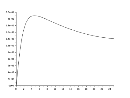
Figure 1: Shape of the function $G$ defined in Theorem 4.1.

Conjecture 4.3 (Shape of $G$).

There exists $r_{c}\sim 4.6$ such that $G^{\prime}(r)>0$ for $r<r_{c}$ and $G^{\prime}(r)<0$ for $r>r_{c}$ and $G(r_{c})\sim 0.2$. Moreover,

$$\lim_{r\to 0}G(r)=0\quad\text{and}\quad\lim_{r\to\infty}G(r)=0.$$

Open question 2 (Shape of the instability domain).

Is it possible to prove Conjecture 4.3? This would imply that the set

$$U_{\alpha}={{\left\{r>0\,:\,{{\left\|X_{t}\right\|}}\xrightarrow[t\to\infty]{p.s.}+\infty\right\}}}={{\left\{r>0\,:\,L(r,\alpha)>0\right\}}}={{\left\{r>0\,:\,G(r)>\alpha\right\}}}$$

is empty for $\alpha>G(r_{c})$ and is a non empty interval if $\alpha<G(r_{c})$.

Remark 4.4 (On the irreducibility of $(U,I)$).

Notice that one can modify the matrices $A_{0}$ and $A_{1}$ in such a way that $(U,I)$ has two ergodic invariant measures (see [9]).

Open question 3 (Oscillations of the Lyapunov exponent).

Is it possible to choose the two $2\times 2$ matrices $A_{0}$ and $A_{1}$ in such a way that the set of jump rates $r$ associated to unstable processes is the union of several intervals?

4.1.2 A deterministic counterpart

Consider the following ODE

$$\dot{x}_{t}=(1-u_{t})A_{0}x_{t}+u_{t}A_{1}x_{t},$$ (10)

where $u$ is a given measurable function from $[0,\infty)$ to ${{\left\{0,1\right\}}}$. The system is said to be unstable if there exists a starting point $x_{0}$ and a measurable function $u$ : $[0,\infty)\to{{\left\{0,1\right\}}}$ such that the solution of (10) goes to infinity.

In [13, 4, 5], the authors provide necessary and sufficient conditions for the solution of (10) to be unbounded for two matrices $A_{0}$ and $A_{1}$ in $\mathcal{M}_{2}(\mathbb{R})$. In the particular case (9), this result reads as follows.

Theorem 4.5 (Criterion for stability [5]).

If $A_{0}$ and $A_{1}$ are given by (9), the system (10) is unbounded if and only if

$$R(\alpha^{2}):=\frac{1+2\alpha^{2}+\sqrt{1+4\alpha^{2}}}{2\alpha^{2}}e^{-2\sqrt{1+4\alpha^{2}}}>1.$$ (11)

More precisely, the result in [5] ensures that

• if $2\alpha>1$ (case $S1$ in [5]) then there exists a common quadratic Lyapunov function for $A_{0}$ and $A_{1}$ (and ${{\left\|X_{t}\right\|}}$ goes to 0 exponentially fast as $t\to\infty$ for any function $u$),

• if $2\alpha\leqslant 1$ (case $S4$ in [5]) then, the system is

  • globally uniformly asymptotically stable (and ${{\left\|X_{t}\right\|}}$ goes to 0 exponentially fast as $t\to\infty$ for any function $u$) if $R(\alpha^{2})<1$,

  • uniformly stable (but for some functions $u$, ${{\left\|X_{t}\right\|}}$ does not converge to 0) if $R(\alpha^{2})=1$,

  • unbounded if $R(\alpha^{2})>1$,

  where $R(\alpha^{2})$ is given by (11).

Proof of Theorem 4.5.

The general case is considered in [5]. The main idea is to construct the so-called worst trajectory choosing at each instant of time the vector field that drives the particle away from the origin. The solutions $x_{t}=(y_{t},z_{t})$ of $\dot{x}_{t}=A_{0}x_{t}$ and $\dot{x}_{t}=A_{1}x_{t}$ starting from $x_{0}=(y_{0},z_{0})$ are respectively given by

$$\begin{cases}y_{t}=(z_{0}t+y_{0})e^{-\alpha t}&\\ z_{t}=z_{0}e^{-\alpha t}\end{cases}\quad\text{and}\quad\begin{cases}y_{t}=y_{0}e^{-\alpha t}&\\ z_{t}=(-y_{0}t+z_{0})e^{-\alpha t}.\end{cases}$$

Let us define, for $x=(y,z)$,

$$Q(x)=\det(A_{0}x,A_{1}x)=\alpha y^{2}-yz-\alpha z^{2}.$$

Then the set of the points where $A_{0}x$ and $A_{1}x$ are collinear is given by

$${{\left\{x\in\mathbb{R}^{2}\ :\ Q(x)=0\right\}}}={{\left\{x=(y,z)\ :\ y=\gamma^{+}z\text{ or }y=\gamma^{-}z\right\}}}$$

where

$$\gamma^{+}=\frac{1+\sqrt{1+4\alpha^{2}}}{2\alpha}>0\quad\text{and}\quad\gamma^{-}=\frac{1-\sqrt{1+4\alpha^{2}}}{2\alpha}<0.$$

Let us start with $x_{0}=(0,1)$ and $I_{0}=0$. Choose $t_{1}=\gamma^{+}$ in such a way that:

$$x_{t_{1}}={{\left(\gamma^{+}e^{-\alpha\gamma^{+}},e^{-\alpha\gamma^{+}}\right)}}.$$

Now, set $t_{2}=t_{1}+\gamma^{+}-\gamma^{-}$ and $I_{t}=1$ for $t\in[t_{1},t_{2})$ in such a way that $y_{t_{2}}=\gamma^{-}z_{t_{2}}$ i.e. $y_{t_{2}}=-(\gamma^{+})^{-1}z_{t_{2}}$. Then, one has

$$x_{t_{2}}={{\left(\gamma^{+}e^{-\alpha(2\gamma^{+}-\gamma^{-})},-(\gamma^{+})^{2}e^{-\alpha(2\gamma^{+}-\gamma^{-})}\right)}}.$$

Finally, choose $t_{3}=t_{2}-\gamma^{-}$ and $I_{t}=0$ for $t\in[t_{2},t_{3})$ in such a way that $y_{t_{3}}=0$. Then, one has

$$x_{t_{3}}={{\left(0,-(\gamma^{+})^{2}e^{-2\alpha(\gamma^{+}-\gamma^{-})}\right)}}.$$

The process is unbounded if and only if ${{\left\|x_{t_{3}}\right\|}}>1$. This is equivalent to (11). ∎

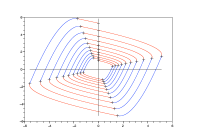
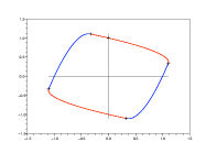
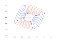
Figure 2: The worth trajectory with $\alpha=0.32$ (on the left), $\alpha=0.3314$ (in the middle) and $\alpha=0.34$ (on the right). The system evolves clock-wisely from $(0,1)$.

4.2 Invariant measure(s) of switched flows

In order to avoid the possible explosions studied in Section 4.1, one can impose that the state space of the continuous variable is a compact set.

In [7], it is shown thanks to an example that the number of the invariant measures may depend on the jump rate for fixed vector fields (as for the problem of (un)-stability described in the previous section). Moreover Hörmander-like conditions on the vector fields are formulated in [2, 7] to ensure that the first marginal of the invariant measure(s) may be absolutely continuous with respect to the Lebesgue measure on $\mathbb{R}^{d}$. However the density may blow up as it is shown in the example below.

Example 4.6 (Possible blow up of the density near a critical point).

Consider the process on $\mathbb{R}\times{{\left\{0,1\right\}}}$ associated to the infinitesimal generator

$$Lf(x,i)=-\alpha_{i}(x-i)\partial_{x}f(x,i)+\lambda_{i}(f(x,1-i)-f(x)).$$

This process is studied in [36, 58]. The support of its invariant measure $\mu$ is the set $[0,1]\times{{\left\{0,1\right\}}}$ and $\mu$ is given by

$$\int f\,d\mu=\frac{\lambda_{1}}{\lambda_{0}+\lambda_{1}}\int_{0}^{1}\!f(x,0)p_{0}(x)\,dx+\frac{\lambda_{0}}{\lambda_{0}+\lambda_{1}}\int_{0}^{1}\!f(x,1)p_{1}(x)\,dx,$$

where $p_{0}$ and $p_{1}$ are Beta distributions:

$$p_{0}(x)=\frac{x^{\lambda_{0}/\alpha_{0}-1}(1-x)^{\lambda_{1}/\alpha_{1}}}{B(\lambda_{0}/\alpha_{0},\lambda_{1}/\alpha_{1}+1)}\quad\text{and}\quad p_{1}(x)=\frac{x^{\lambda_{0}/\alpha_{0}}(1-x)^{\lambda_{1}/\alpha_{1}-1}}{B(\lambda_{0}/\alpha_{0}+1,\lambda_{1}/\alpha_{1})}.$$

The density of the invariant measure possibly explodes near 0 or 1.

The paper [3] is a detailed analysis of invariant measures for switched flows in dimension one. In particular, the authors prove smoothness of the invariant densities away from critical points and describe the asymptotics of the invariant densities at critical points.

The situation is more intricate for higher dimensions.

Example 4.7 (Possible blow up of the density in the interior of the support).

Consider the process on $\mathbb{R}^{2}\times{{\left\{0,1\right\}}}$ associated to the constant jump rates $\lambda_{0}$ and $\lambda_{1}$ for the discrete component and the vector fields

$$F^{0}(x)=Ax\text{ and }F^{1}(x)=A(x-a)\text{ where }A=\begin{pmatrix}-1&-1\\ 1&-1\end{pmatrix}\quad\text{and}\quad a=\begin{pmatrix}1\\ 0\end{pmatrix}.$$ (12)

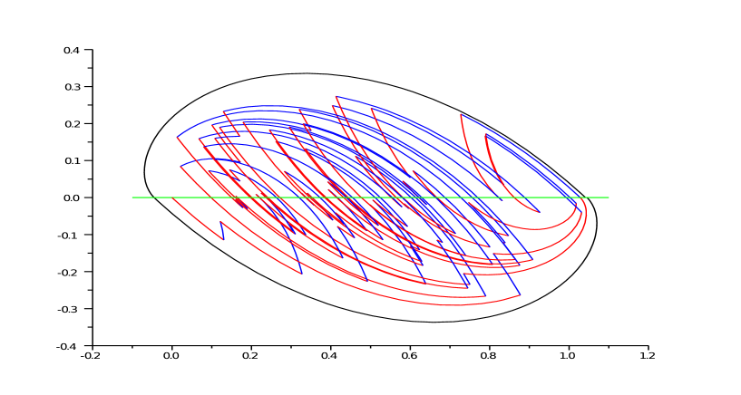
Figure 3: Path of the process associated to $F^{0}$ and $F^{1}$ given by (12) starting from the origin. Red (resp. blue) pieces of path correspond to $I=1$ (resp. $I=0$).

The origin and $a$ are the respective unique critical points of $F^{0}$ and $F^{1}$. Thanks to the precise estimates in [3], one can prove the following fact. If $\lambda_{0}$ is small enough then, as for one-dimensional example, the density of the invariant measure blows up at the origin. This also implies that the density is infinite on the set ${{\left\{\varphi^{1}_{t}(0)\ :\ t\geqslant 0\right\}}}$.

Open question 4.

What can be said on the smoothness of the density of the invariant measure of such processes?

4.3 A convergence result

This section sums up the study of the long time behavior of certain switched flows presented in [8]. See also [61] for another approach. To focus on the main lines of this paper, the hypotheses below are far from the optimal ones.

Hypothesis 4.8 (Regularity of the jump rates).

There exist $\underline{a}>0$ and $\kappa>0$ such that, for any $x,\tilde{x}\in\mathbb{R}^{d}$ and $i,j\in E$,

$$a(x,i,j)\geqslant\underline{a}\quad\text{and}\quad\sum_{j\in E}{{\left|a(x,i,j)-a(\tilde{x},i,j)\right|}}\leqslant\kappa{{\left\|x-\tilde{x}\right\|}}.$$

The lower bound condition insures that the second — discrete — coordinate of $Z$ changes often enough (so that the second coordinates of two independent copies of $Z$ coincide sufficiently often).

Hypothesis 4.9 (Strong dissipativity of the vector fields).

There exists $\alpha>0$ such that,

$${{\left<x-\tilde{x},F^{i}(x)-F^{i}(\tilde{x})\right>}}\leqslant-\alpha{{\left\|x-\tilde{x}\right\|}}^{2},\quad x,\tilde{x}\in\mathbb{R}^{d},\ i\in E.$$ (13)

Hypothesis 4.9 ensures that, for any $i\in E$,

$${{\left\|\varphi^{i}_{t}(x)-\varphi^{i}_{t}(\tilde{x})\right\|}}\leqslant e^{-\alpha t}{{\left\|x-\tilde{x}\right\|}},\quad x,\tilde{x}\in\mathbb{R}^{d}.$$

As a consequence, the vector fields $F^{i}$ has exactly one critical point $\sigma(i)\in\mathbb{R}^{d}$. Moreover it is exponentially stable since, for any $x\in\mathbb{R}^{d}$,

$${{\left\|\varphi^{i}_{t}(x)-\sigma(i)\right\|}}\leqslant e^{-\alpha t}{{\left\|x-\sigma(i)\right\|}}.$$

In particular, $X$ cannot escape from a sufficiently large ball $\bar{B}(0,M)$. Define the following distance $\mathcal{W}_{1}$ on the probability measures on $B(0,M)\times E$: for $\eta,\tilde{\eta}\in\mathcal{P}(B(0,M)\times E)$,

$$\mathcal{W}_{1}(\eta,\tilde{\eta})=\inf{{\left\{\mathbb{E}|X-\tilde{X}|+\mathbb{P}(I\neq\tilde{I})\,:\,(X,I)\sim\eta\text{ and }(\tilde{X},\tilde{I})\sim\tilde{\eta}\right\}}}.$$

Theorem 4.10 (Long time behavior [8]).

Assume that Hypotheses 4.8 and 4.9 hold.

Then, the process has a unique invariant measure and its support is included in $\bar{B}(0,M)\times E$. Moreover, let $\nu_{0}$ and $\tilde{\nu}_{0}$ be two probability measures on $\bar{B}(0,M)\times E$. Denote by $\nu_{t}$ the law of $Z_{t}$ when $Z_{0}$ is distributed as $\nu_{0}$ Then there exist positive constants $c$ and $\gamma$ such that

$$\mathcal{W}_{1}{{\left(\eta_{t},\tilde{\eta}_{t}\right)}}\leqslant ce^{-\gamma t}.$$

The constants $c$ and $\gamma$ can be explicitly expressed in term of the parameters of the model (see [8]). The proof relies on the construction of an explicit coupling. See also [17, 48].

Open question 5.

One can apply Theorem 4.10 to the processes defined in Examples 4.6 and 4.7. The associated time reversal processes are associated to unstable vector fields and unbounded jump rates. What can be said about their convergence to equilibrium?

Section 4.4 present an application of this theorem to a biological model. In Section 4.5, we describe a naïve model for the movement of bacteria that can also be seen as an ergodic telegraph process.

4.4 Neuron activity

The paper [55] establishes limit theorems for a class of stochastic hybrid systems (continuous deterministic dynamic coupled with jump Markov processes) in the fluid limit (small jumps at high frequency), thus extending known results for jump Markov processes. The main results are a functional law of large numbers with exponential convergence speed, a diffusion approximation, and a functional central limit theorem. These results are then applied to neuron models with stochastic ion channels, as the number of channels goes to infinity, estimating the convergence to the deterministic model. In terms of neural coding, the central limit theorems allows to estimate numerically the impact of channel noise both on frequency and spike timing coding.

The Morris–Lecar model introduced in [49] describes the evolution in time of the electric potential $V(t)$ in a neuron. The neuron exchanges different ions with its environment via ion channels which may be open or closed. In the original – deterministic – model, the proportion of open channels of different types are coded by two functions $m(t)$ and $n(t)$, and the three quantities $m$, $n$ and $V$ evolve through the flow of an ordinary differential equation.

Various stochastic versions of this model exist. Here we focus on a model described in [63], to which we refer for additional information. This model is motivated by the fact that $m$ and $n$, being proportions of open channels, are better coded as discrete variables. More precisely, we fix a large integer $K$ (the total number of channels) and define a PDMP $(V,u_{1},u_{2})$ with values in $\mathbb{R}\times\{0,1/K,2/K\dots,1\}^{2}$ as follows.

Firstly, the potential $V$ evolves according to

$$\frac{dV(t)}{dt}=\frac{1}{C}\left(I-\sum_{i=1}^{3}g_{i}u_{i}(t)(V-V_{i})\right)$$ (14)

where $C$ and $I$ are positive constants (the capacitance and input current), the $g_{i}$ and $V_{i}$ are positive constants (representing conductances and equilibrium potentials for different types of ions), $u_{3}(t)$ is equal to $1$ and $u_{1}(t)$, $u_{2}(t)$ are the (discrete) proportions of open channels for two types of ions.

These two discrete variables follow birth-death processes on $\{0,1/K,\ldots,1\}$ with birth rates $\alpha_{1}$, $\alpha_{2}$ and death rates $\beta_{1}$, $\beta_{2}$ that depend on the potential $V$:

$$\alpha_{i}(V) =c_{i}\cosh\left(\frac{V-V^{\prime}_{i}}{2V^{\prime\prime}_{i}}\right)\left(1+\tanh\left(\frac{V-V^{\prime}_{i}}{V^{\prime\prime}_{i}}\right)\right)$$ (15)

$$\beta_{i}(V) =c_{i}\cosh\left(\frac{V-V^{\prime}_{i}}{2V^{\prime\prime}_{i}}\right)\left(1-\tanh\left(\frac{V-V^{\prime}_{i}}{V^{\prime\prime}_{i}}\right)\right)$$

where the $c_{i}$ and $V^{\prime}_{i}$, $V^{\prime\prime}_{i}$ are constants.

Let us check that Theorem 4.10 can be applied in this example. Formally the process is a PDMP with $d=1$ and the finite set $E=\{0,1/K,\ldots,1\}^{2}$. The discrete process $(u_{1},u_{2})$ plays the role of the index $i\in E$, and the fields $F^{(u_{1},u_{2})}$ are defined (on $\mathbb{R}$) by (14) by setting $u_{1}(t)=u_{1}$, $u_{2}(t)=u_{2}$.

The constant term $u_{3}g_{3}$ in (14) ensures that the uniform dissipation property (13) is satisfied: for all $(u_{1},u_{2})$,

$${{\left<V-\tilde{V},F^{(u_{1},u_{2})}(V)-F^{(u_{1},u_{2})}(\tilde{V})\right>}} =-\frac{1}{C}\sum_{i=1}^{3}u_{i}g_{i}(V-\tilde{V})^{2}$$

$$\leqslant-\frac{1}{C}u_{3}g_{3}(V-\tilde{V})^{2}.$$

The Lipschitz character and the bound from below on the rates are not immediate. Indeed the jump rates (15) are not bounded from below if $V$ is allowed to take values in $\mathbb{R}$.

However, a direct analysis of (14) shows that $V$ is essentially bounded : all the fields $F^{(u_{1},u_{2})}$ point inward at the boundary of the (fixed) line segment $\mathcal{S}=[0,\max(V_{1},V_{2},V_{3}+(I+1)/g_{3}u_{3})]$, so if $V(t)$ starts in this region it cannot get out. The necessary bounds all follow by compactness, since $\alpha_{i}(V)$ and $\beta_{i}(V)$ are $\mathcal{C}^{1}$ in $\mathcal{S}$ and strictly positive.

4.5 Chemotaxis

Let us briefly describe how bacteria move (see [50, 26, 25] for details). They alternate two basic behavioral modes: a more or less linear motion, called a run, and a highly erratic motion, called tumbling, the purpose of which is to reorient the cell. During a run the bacteria move at approximately constant speed in the most recently chosen direction. Run times are typically much longer than the time spent tumbling. In practice, the tumbling time is neglected. An appropriate stochastic process for describing the motion of cells is called the velocity jump process which is deeply studied in [50]. The velocity belongs to a compact set (the unit sphere for example) and changes by random jumps at random instants of time. Then, the position is deduced by integration of the velocity. The jump rates may depend on the position when the medium is not homogeneous: when bacteria move in a favorable direction i.e. either in the direction of foodstuffs or away from harmful substances the run times are increased further. Sometimes, a diffusive approximation is available [50, 60].

In the one-dimensional simple model studied in [27], the particle evolves in $\mathbb{R}$ and its velocity belongs to ${{\left\{-1,+1\right\}}}$. Its infinitesimal generator is given by:

$$Af(x,v)=v\partial_{x}f(x,v)+{{\left(a+(b-a)\mathds{1}_{{\left\{xv>0\right\}}}\right)}}(f(x,-v)-f(x,v)),$$ (16)

with $0<a<b$. The dynamics of the process is simple: when $X$ goes aways from 0, (resp. goes to 0), $V$ flips to $-V$ with rate $b$ (resp. $a)$. Since $b>a$, it is quite intuitive that this Markov process is ergodic. One could think about it as an analogue of the diffusion process solution of

$$dZ_{t}=dB_{t}-\text{sign}(Z_{t})\,dt.$$

More precisely, under a suitable scaling, one can show that $X$ goes to $Z$. Finally, this process is an ergodic version of the so-called telegraph process. See for example [35, 32].

Of course, this process does not satisfy the hypotheses of Theorem 4.10 since the vector fields have no stable point. It is shown in [27] that the invariant measure $\mu$ of $(X,V)$ driven by (16) is the product measure on $\mathbb{R}_{+}\times{{\left\{-1,+1\right\}}}$ given by

$$\mu(dx,dv)=(b-a)e^{-(b-a)x}\,dx\otimes\frac{1}{2}(\delta_{-1}+\delta_{+1})(dv).$$

One can also construct an explicit coupling to get explicit bounds for the convergence to the invariant measure in total variation norm [27]. See also [47] for another approach, linked with functional inequalities.

Open question 6 (More realistic models).

Is it possible to establish quantitative estimates for the convergence to equilibrium for more realistic dynamics (especially in $\mathbb{R}^{3}$) as considered in [50, 26, 25]?

Acknowledgements.

FM deeply thanks Persi Diaconis for his energy, curiosity and enthusiasm and Laurent Miclo for the perfect organisation of the stimulating workshop "Talking Across Fields" in Toulouse during March 2014. This paper has been improved thanks to the constructive comments of two referees. FM acknowledges financial support from the French ANR project ANR-12-JS01-0006 - PIECE.

Florent Malrieu, e-mail: florent.malrieu(AT)univ-tours.fr

Laboratoire de Mathématiques et Physique Théorique (UMR CNRS 6083), Fédération Denis Poisson (FR CNRS 2964), Université François-Rabelais, Parc de Grandmont, 37200 Tours, France.

References

- [1] D. Aldous and P. Diaconis, Strong uniform times and finite random walks, Adv. in Appl. Math. 8 (1987), no. 1, 69–97. MR 876954 (88d:60175)
- [2] Y. Bakhtin and T. Hurth, Invariant densities for dynamical systems with random switching, Nonlinearity 25 (2012), no. 10, 2937–2952.
- [3] Y. Bakhtin, T. Hurth, and J. C. Mattingly, Regularity of invariant densities for 1D-systems with random switching, arXiv:1406.5425, 2014.
- [4] M. Balde and U. Boscain, Stability of planar switched systems: the nondiagonalizable case, Commun. Pure Appl. Anal. 7 (2008), no. 1, 1–21. MR 2358351 (2009b:93133)
- [5] M. Balde, U. Boscain, and P. Mason, A note on stability conditions for planar switched systems, Internat. J. Control 82 (2009), no. 10, 1882–1888. MR 2567235 (2010i:93122)
- [6] J.-B. Bardet, A. Christen, A. Guillin, A. Malrieu, and P.-A. Zitt, Total variation estimates for the TCP process, Electron. J. Probab. 18 (2013), no. 10, 1–21.
- [7] M. Benaïm, S. Le Borgne, F. Malrieu, and P.-A. Zitt, Qualitative properties of certain piecewise deterministic Markov processes, To appear in Ann. Inst. Henri Poincaré Probab. Stat., arXiv:1204.4143, 2012.
- [8] , Quantitative ergodicity for some switched dynamical systems, Electron. Commun. Probab. 17 (2012), no. 56, 14. MR 3005729
- [9] , On the stability of planar randomly switched systems, Ann. Appl. Probab. 24 (2014), no. 1, 292–311. MR 3161648
- [10] J. Berestycki, J. Bertoin, B. Haas, and G. Miermont, Quelques aspects fractals des fragmentations aléatoires, Quelques interactions entre analyse, probabilités et fractals, Panor. Synthèses, vol. 32, Soc. Math. France, Paris, 2010, pp. 191–243. MR 2932439
- [11] P. Bertail, S. Clémençon, and J. Tressou, A storage model with random release rate for modeling exposure to food contaminants, Math. Biosci. Eng. 5 (2008), no. 1, 35–60. MR 2401278 (2009e:92008)
- [12] M. Borkovec, A. Dasgupta, S. Resnick, and G. Samorodnitsky, A single channel on/off model with TCP-like control, Stoch. Models 18 (2002), no. 3, 333–367.
- [13] U. Boscain, Stability of planar switched systems: the linear single input case, SIAM J. Control Optim. 41 (2002), no. 1, 89–112. MR 1920158 (2003h:93066)
- [14] F. Bouguet, Quantitative exponential rates of convergence for exposure to food contaminants, To appear in ESAIM PS, arXiv:1310.3948, 2013.
- [15] V. Calvez, M. Doumic Jauffret, and P. Gabriel, Self-similarity in a general aggregation-fragmentation problem. Application to fitness analysis, J. Math. Pures Appl. (9) 98 (2012), no. 1, 1–27. MR 2935368
- [16] D. Chafaï, F. Malrieu, and K. Paroux, On the long time behavior of the TCP window size process, Stochastic Process. Appl. 120 (2010), no. 8, 1518–1534. MR 2653264
- [17] B. Cloez and M. Hairer, Exponential ergodicity for markov processes with random switching, To appear in Bernoulli Journal, 2014.
- [18] F. Comets, S. Popov, G. M. Schütz, and M. Vachkovskaia, Billiards in a general domain with random reflections, Arch. Ration. Mech. Anal. 191 (2009), no. 3, 497–537. MR 2481068 (2010h:37077)
- [19] A. Crudu, A. Debussche, A. Muller, and O. Radulescu, Convergence of stochastic gene networks to hybrid piecewise deterministic processes, Ann. Appl. Probab. 22 (2012), no. 5, 1822–1859. MR 3025682
- [20] M. H. A. Davis, Piecewise-deterministic Markov processes: a general class of nondiffusion stochastic models, J. Roy. Statist. Soc. Ser. B 46 (1984), no. 3, 353–388, With discussion. MR MR790622 (87g:60062)
- [21] , Markov models and optimization, Monographs on Statistics and Applied Probability, vol. 49, Chapman & Hall, London, 1993.
- [22] P. Diaconis and D. Freedman, Iterated random functions, SIAM Rev. 41 (1999), no. 1, 45–76. MR 1669737 (2000c:60102)
- [23] M. Doumic Jauffret and P. Gabriel, Eigenelements of a general aggregation-fragmentation model, Math. Models Methods Appl. Sci. 20 (2010), no. 5, 757–783. MR 2652618 (2011d:35055)
- [24] V. Dumas, F. Guillemin, and Ph. Robert, A Markovian analysis of additive-increase multiplicative-decrease algorithms, Adv. in Appl. Probab. 34 (2002), no. 1, 85–111. MR MR1895332 (2003f:60168)
- [25] R. Erban and H. G. Othmer, From individual to collective behavior in bacterial chemotaxis, SIAM J. Appl. Math. 65 (2004/05), no. 2, 361–391 (electronic).
- [26] , From signal transduction to spatial pattern formation in E. coli: a paradigm for multiscale modeling in biology, Multiscale Model. Simul. 3 (2005), no. 2, 362–394 (electronic).
- [27] Joaquin Fontbona, Hélène Guérin, and Florent Malrieu, Quantitative estimates for the long-time behavior of an ergodic variant of the telegraph process, Adv. in Appl. Probab. 44 (2012), no. 4, 977–994. MR 3052846
- [28] S. Gadat and L. Miclo, Spectral decompositions and -operator norms of toy hypocoercive semi-groups, Kinet. Relat. Models 6 (2013), no. 2, 317–372. MR 3030715
- [29] C. Graham and Ph. Robert, Interacting multi-class transmissions in large stochastic networks, Ann. Appl. Probab. 19 (2009), no. 6, 2334–2361.
- [30] , Self-adaptive congestion control for multiclass intermittent connections in a communication network, Queueing Syst. 69 (2011), no. 3-4, 237–257. MR 2886470
- [31] F. Guillemin, Ph. Robert, and B. Zwart, AIMD algorithms and exponential functionals, Ann. Appl. Probab. 14 (2004), no. 1, 90–117.
- [32] S. Herrmann and P. Vallois, From persistent random walk to the telegraph noise, Stoch. Dyn. 10 (2010), no. 2, 161–196.
- [33] J. P. Hespanha, A model for stochastic hybrid systems with application to communication networks, Nonlinear Anal. 62 (2005), no. 8, 1353–1383.
- [34] M. Jacobsen, Point process theory and applications, Probability and its Applications, Birkhäuser Boston Inc., Boston, MA, 2006, Marked point and piecewise deterministic processes. MR 2189574 (2007a:60001)
- [35] M. Kac, A stochastic model related to the telegrapher’s equation, Rocky Mountain J. Math. 4 (1974), 497–509.
- [36] R. Karmakar and I. Bose, Graded and binary responses in stochastic gene expression, Physical Biology 197 (2004), no. 1, 197–214.
- [37] D. Lamberton and G. Pagès, A penalized bandit algorithm, Electron. J. Probab. 13 (2008), no. 13, 341–373. MR 2386736 (2009a:62328)
- [38] S. D. Lawley, J. C. Mattingly, and M. C. Reed, Sensitivity to switching rates in stochastically switched ODEs, Commun. Math. Sci. 12 (2014), no. 7, 1343–1352. MR 3210750
- [39] J. S. H. van Leeuwaarden and A. H. Löpker, Transient moments of the TCP window size process, J. Appl. Probab. 45 (2008), no. 1, 163–175.
- [40] J. S. H. van Leeuwaarden, A. H. Löpker, and T. J. Ott, TCP and iso-stationary transformations, Queueing Syst. 63 (2009), no. 1-4, 459–475.
- [41] D. A. Levin, Y. Peres, and E. L. Wilmer, Markov chains and mixing times, American Mathematical Society, Providence, RI, 2009, With a chapter by James G. Propp and David B. Wilson. MR 2466937 (2010c:60209)
- [42] M. C. Mackey, M. Tyran-Kamińska, and R. Yvinec, Dynamic behavior of stochastic gene expression models in the presence of bursting, SIAM J. Appl. Math. 73 (2013), no. 5, 1830–1852. MR 3097042
- [43] K. Maulik and B. Zwart, Tail asymptotics for exponential functionals of Lévy processes, Stochastic Process. Appl. 116 (2006), no. 2, 156–177.
- [44] , An extension of the square root law of TCP, Ann. Oper. Res. 170 (2009), 217–232. MR 2506283 (2010d:94010)
- [45] L. Miclo and P. Monmarché, Étude spectrale minutieuse de processus moins indécis que les autres, Séminaire de Probabilités XLV, Lecture Notes in Math., vol. 2078, Springer, Cham, 2013, pp. 459–481. MR 3185926
- [46] S. Mischler and J. Scher, Spectral analysis of semigroups and growth-fragmentation equations, arXiv:1310.7773, 2013.
- [47] P. Monmarché, Hypocoercive relaxation to equilibrium for some kinetic models, Kinet. Relat. Models 7 (2014), no. 2, 341–360. MR 3195078
- [48] P. Monmarché, On and entropic convergence for contractive PDMP, arXiv:1404.4220, 2014.
- [49] C. Morris and H. Lecar, Voltage oscillations in the barnacle giant muscle fiber, Biophys. J. 35 (1981), no. 1, 193–213.
- [50] H. G. Othmer, S. R. Dunbar, and W. Alt, Models of dispersal in biological systems, J. Math. Biol. 26 (1988), no. 3, 263–298.
- [51] T. J. Ott, Rate of convergence for the ‘square root formula’ in the internet transmission control protocol, Adv. in Appl. Probab. 38 (2006), no. 4, 1132–1154.
- [52] T. J. Ott and J. H. B. Kemperman, Transient behavior of processes in the TCP paradigm, Probab. Engrg. Inform. Sci. 22 (2008), no. 3, 431–471.
- [53] T. J. Ott, J. H. B. Kemperman, and M. Mathis, The stationary behavior of ideal TCP congestion avoidance, unpublished manuscript available at http://www.teunisott.com/, 1996.
- [54] T. J. Ott and J. Swanson, Asymptotic behavior of a generalized TCP congestion avoidance algorithm, J. Appl. Probab. 44 (2007), no. 3, 618–635.
- [55] K. Pakdaman, M. Thieullen, and G. Wainrib, Fluid limit theorems for stochastic hybrid systems with application to neuron models, Adv. in Appl. Probab. 42 (2010), no. 3, 761–794. MR 2779558 (2011m:60070)
- [56] B. Perthame, Transport equations in biology, Frontiers in Mathematics, Birkhäuser Verlag, Basel, 2007. MR 2270822 (2007j:35004)
- [57] B. Perthame and L. Ryzhik, Exponential decay for the fragmentation or cell-division equation, J. Differential Equations 210 (2005), no. 1, 155–177. MR 2114128 (2006b:35328)
- [58] O. Radulescu, A. Muller, and A. Crudu, Théorèmes limites pour des processus de Markov à sauts. Synthèse des résultats et applications en biologie moléculaire, Technique et Science Informatiques 26 (2007), no. 3-4, 443–469.
- [59] G. O. Roberts and R. L. Tweedie, Rates of convergence of stochastically monotone and continuous time Markov models, J. Appl. Probab. 37 (2000), no. 2, 359–373. MR 1780996 (2001i:60111)
- [60] M. Rousset and G. Samaey, Individual-based models for bacterial chemotaxis in the diffusion asymptotics, Math. Models Methods Appl. Sci. 23 (2013), no. 11, 2005–2037. MR 3084742
- [61] J. Shao, Ergodicity of regime-switching diffusions in Wasserstein distances, arXiv 1403.0291, 2014.
- [62] C. Villani, Topics in optimal transportation, Graduate Studies in Mathematics, vol. 58, American Mathematical Society, Providence, RI, 2003. MR MR1964483 (2004e:90003)
- [63] G. Wainrib, M. Thieullen, and K. Pakdaman, Intrinsic variability of latency to first-spike, Biol. Cybernet. 103 (2010), no. 1, 43–56. MR 2658681
- [64] G. G. Yin and C. Zhu, Hybrid switching diffusions, Stochastic Modelling and Applied Probability, vol. 63, Springer, New York, 2010, Properties and applications. MR 2559912 (2010i:60226)
- [65] R. Yvinec, C. Zhuge, J. Lei, and M. C. Mackey, Adiabatic reduction of a model of stochastic gene expression with jump Markov process, J. Math. Biol. 68 (2014), no. 5, 1051–1070. MR 3175198