Higher-order Spatial Accuracy in Diffeomorphic Image Registration

Henry O. Jacobslabel=e1]h.jacobs@imperial.ac.uk [ Department of Mathematics
Imperial College
London SW7 2AZ, UK
   Stefan Sommerlabel=e2]sommer@di.ku.dk [ Department of Computer Science
University of Copenhagen
Universitetsparken 1, DK-2100
Copenhagen E, Denmark
(2014)
Abstract

We discretize a cost functional for image registration problems by deriving Taylor expansions for the matching term. Minima of the discretized cost functionals can be computed with no spatial discretization error, and the optimal solutions are equivalent to minimal energy curves in the space of k𝑘k-jets. We show that the solutions convergence to optimal solutions of the original cost functional as the number of particles increases with a convergence rate of O(hd+k)𝑂superscript𝑑𝑘O(h^{d+k}) where hh is a resolution parameter. The effect of this approach over traditional particle methods is illustrated on synthetic examples and real images.

volume: 0issue: 0
\startlocaldefs\endlocaldefs

and

1 Introduction

The goal of image registration is to place differing images of the same object (e.g. MRI scans) into a shared coordinate system so that they may be compared. One common means of doing this is to deform one image until it matches the other. Typical numerical schemes for implementing this task are particle methods, where particles are used as a finite dimensional representation of a diffeomorphism. If the particles are initialized on a regular grid of resolution hh, then the solutions can be O(hd)𝑂superscript𝑑O(h^{d}) accurate at best where d𝑑d is the dimension of the image domain. Improving this order of accuracy is non-trivial because traditional higher-order numerical schemes are designed on fixed meshes (e.g. higher order finite differences).

In this paper, we seek to improve this order of accuracy by considering a more sophisticated class of particles. We will find that by equipping the particles with jet-data, one can achieve registrations with higher orders of accuracy. One impact of the use of higher-order particles is that the improved accuracy per particle permits the use of fewer particles for a desired total accuracy. For sufficiently smooth initial data, this implies the storage requirements are improved as well.

1.1 Organization of the paper

We will introduce the higher-order accurate image registration framework through the following steps:

  1. 1.

    We will introduce the hierarchy of jet-particles.

  2. 2.

    We will pose an image registration problem as an optimal control problem on an infinite dimensional space.

  3. 3.

    We will pose a sequence of deformed problems which are easier to solve.

  4. 4.

    We will reduce the deformed optimization problems to optimization problems involving computation of finite dimensional ODEs (i.e. an infinite dimensional reduction).

  5. 5.

    We will find necessary conditions for sequences of computed solutions to the deformed problems to converge to the solution of the original problem at a rate O(hd+k)𝑂superscript𝑑𝑘O(h^{d+k}), where k0𝑘0k\geq 0 depends on the order of the jet-particles used.

Finally, we will display the results of numerical experiments comparing the use of zeroth, first, and second order jet-particles.

2 Previous work

In this section, we attempt a brief overview of the large deformation diffeomorphic metric mapping (LDDMM) framework from its origins in the 1990s, to its recent marriage with geometric mechanics (2000s-present).

2.1 Matching with LDDMM

The notion of seeking deformations for the sake of image registration goes back a long way, see [SDP13, You10] and references therein. One of the first attempts was to consider diffeomorphisms of the form φ(x)=x+f(x)𝜑𝑥𝑥𝑓𝑥\varphi(x)=x+f(x) for some map f:dd:𝑓superscript𝑑superscript𝑑f:\mathbb{R}^{d}\to\mathbb{R}^{d}. The map f𝑓f is often denoted a displacement field. When f𝑓f is “small”, φ𝜑\varphi is a diffeomorphism, but this can fail when f𝑓f is “large” [You10, Chapter 7]. Many algorithms outside the LDDMM context employ a small deformation approach with a displacement field f𝑓f. The displacement can be represented for example with B-spline basis functions. Particle methods, as considered in this paper, can loosely be interpreted as large deformation equivalents to representing the displacement f𝑓f with finite linear combinations of basis functions. In particular, the kernel K𝐾K can be thought of as taking the role of e.g. B-spline basis functions in small deformation approaches.

The breakdown for large f𝑓f is a result of the fact that the space of diffeomorphisms is a nonlinear space. One of the early obstacles in diffeomorphic image registration entailed dealing with this nonlinearity. A key insight in getting a handle on the nonlinearity of the diffeomorphisms was to consider the linear space of vector fields. Given a time-dependent vector field v(t)𝑣𝑡v(t), one can integrate it to obtain a diffeomorphism φtsubscript𝜑𝑡\varphi_{t}, which is called the flow of v𝑣v [CRM96]. This insight was used to obtain diffeomorphisms for imaging applications by posing an optimal control problem on the space of vector-fields, and then integrating the flow of the optimal vector field to obtain a diffeomorphism. The well-posedness of this approach was studied in [Tro95, DGM98], where the cost functional (i.e. the norm) was identified as a fundamental choice in ensuring well-posedness and controlling properties of the resulting diffeomorphisms. A particle method based upon [DGM98] was implemented for the purpose of medical imaging in [JM00]. The completeness of the Euler-Lagrange equations in [DGM98] was studied thoroughly in [TY05], where the image data was allowed to be of a fairly general type (i.e. any entity upon which diffeomorphisms act smoothly). The analytic safe-guards provided by [DGM98] and [TY05] where then excercised in [BMTY05], where a number of examples were numerically investigated.

2.2 Connections with geometric mechanics

Following these early investigations, connections with geometric mechanics began to form. The cost functional chosen in [JM00] was the H1superscript𝐻1H^{1}-norm of the vector-fields. Coincidentally, this is the cost functional of the n𝑛n-dimensional Camassa-Holm equation (see [HM05] and references therein). In 1-dimension, the particle solutions in [JM00] are identical to the peakon solutions discovered in [CH93], and the numerical scheme reduces to that of [HR06]. The convergence of [JM00] was proven using geometric techniques in [HR06] in the one-dimensional case. The same proof was used in [CDTM12] for arbitrary dimensions. As images appear as advected quantities, the use of momentum maps became a useful conceptual technique for geometers to understand the numerical scheme of [BMTY05]. The identification of numerous mathematical terms in [BMTY05] as momentum maps was performed in [BGBHR11].

2.3 Jet particles

The particle method implemented in [JM00] allowed only for deformations that acted as “local translations” (see Figure 1(a)). Motivated by a desire to create more general deformations [SNDP13] introduced a hierarchy of particles which advect jet-data. We call the particles jet-particles in this paper. The first order jet-particles modify the Jacobian matrix at the particle locations and allow for “locally linear” transformations such as local scalings and local rotations (see Figure 1(b-e)). Second order jet-particles allow for deformations which are “locally quadratic” (i.e. transformations with nontrivial Hessians (see Figure 1(f-h)). The geometric and hierarchal structure of [SNDP13] was investigated in [Jac13] where the Lie groupoid structure of jet-particles was linked to the Lie group structure of the diffeomorphism group, thus making the case for jet-particles as multi-scale representations of diffeomorphisms. Independently, an incompressible version of this idea was invented for the purpose of incompressible fluid modelling in [DJR13]. Solutions to this fluid model were numerically computed in [CHJM14] based upon the regularized Euler fluid equations developed in [MM13] and expressions for matrix-valued reproducing kernels derived in [MG14]. The final section of [CHJM14] provides formulas which illustrate how jet-particles in the k𝑘kth level of the hierarchy yield deformations which are approximated by particles in the (k1)𝑘1(k-1)th level of the hierarchy. The approximation being accurate to an order O(hk)𝑂superscript𝑘O(h^{k}) where h>00h>0 is some measure of particle spacing. This approximation is more or less equivalent to the approximation of a partial differential operator by a finite differences, and it will serve as one of the main tools used in this paper in producing higher-order accurate numerical schemes.

Refer to caption
(a) translation
Refer to caption
(b) expansion
Refer to caption
(c) rotation
Refer to caption
(d) stretch
Refer to caption
(e) shear
Refer to caption
(f) 2nd order
Refer to caption
(g) 2nd order
Refer to caption
(h) 2nd order
Figure 1: Deformations of initially square grids. (a) zeroth order, (b-e) first order, (f-h) second order. A single jet-particle is located at the blue dots before moving with the flows to the red crosses. Grids are colored by log-Jacobian determinant.

3 LDDMM

Let M𝑀M be a manifold and let V𝔛(M)𝑉𝔛𝑀V\subset\mathfrak{X}(M) be a subspace of the vector-fields on M𝑀M equipped with an inner-product ,V:V×V:subscript𝑉𝑉𝑉\langle\cdot,\cdot\rangle_{V}:V\times V\to\mathbb{R}. Let GVDiff(n)subscript𝐺𝑉Diffsuperscript𝑛G_{V}\subset\operatorname{Diff}(\mathbb{R}^{n}) be the corresponding topological Lie group to which V𝑉V integrates [You10, Chapter 8]. To do image registration, we try to assemble a “small” diffeomorphism by minimizing a cost function on the space of curve in GVsubscript𝐺𝑉G_{V}. The standard cost function takes a time-dependent diffeomorphism, φtsubscript𝜑𝑡\varphi_{t}, and outputs a real number. Mathematically, the cost function is often taken to be a map EGV:C1([0,1]:GV)E_{G_{V}}:C^{1}([0,1]:G_{V})\to\mathbb{R} given by

EGV[φ()]:=1201(v(t))𝑑t+F(φ1),assignsubscript𝐸subscript𝐺𝑉delimited-[]𝜑12superscriptsubscript01𝑣𝑡differential-d𝑡𝐹subscript𝜑1\displaystyle E_{G_{V}}[\varphi(\cdot)]:=\frac{1}{2}\int_{0}^{1}\ell(v(t))dt+F(\varphi_{1}),

where v(t)V𝑣𝑡𝑉v(t)\in V is the Eulerian velocity field v(t,x)=tφt(φt1(x))𝑣𝑡𝑥subscript𝑡subscript𝜑𝑡superscriptsubscript𝜑𝑡1𝑥v(t,x)=\partial_{t}\varphi_{t}(\varphi_{t}^{-1}(x)) and \ell is a “control-cost”. Explicitly, φtGVsubscript𝜑𝑡subscript𝐺𝑉\varphi_{t}\in G_{V} is obtained from v(t)V𝑣𝑡𝑉v(t)\in V via the initial value problem

{ddtφt=v(t)φtφ0=id.cases𝑑𝑑𝑡subscript𝜑𝑡𝑣𝑡subscript𝜑𝑡otherwisesubscript𝜑0𝑖𝑑otherwise\displaystyle\begin{cases}\frac{d}{dt}\varphi_{t}=v(t)\circ\varphi_{t}\\ \varphi_{0}=id\end{cases}. (1)

One then obtains extremizers of EGVsubscript𝐸subscript𝐺𝑉E_{G_{V}} by solving the Euler-Lagrange equations on GVsubscript𝐺𝑉G_{V}. However, GVsubscript𝐺𝑉G_{V} is a non-commutative group, and can be very difficult to work with. It is typical to express EGVsubscript𝐸subscript𝐺𝑉E_{G_{V}} as a cost function on the vector-space V𝑉V and incorporate (1) as a constraint. This means optimizing a cost function E:C1([0,1],V):𝐸superscript𝐶101𝑉E:C^{1}([0,1],V)\to\mathbb{R} with respect to constrained variations. Any extremizer, v()𝑣v(\cdot), of E𝐸E must necessarily satisfy a symmetry reduced form of the Euler-Lagrange equations, known as the Euler-Poincaré equation. In essence, the Euler-Poincaré equations are nothing but the Euler-Lagrange equations pulled to the space V𝑉V. For a generic \ell, the Euler-Poincaré equations take the form

ddt(δδv)+adv(δδv)=0.𝑑𝑑𝑡𝛿𝛿𝑣subscriptsuperscriptad𝑣𝛿𝛿𝑣0\displaystyle\frac{d}{dt}\left(\frac{\delta\ell}{\delta v}\right)+\operatorname{ad}^{*}_{v}\left(\frac{\delta\ell}{\delta v}\right)=0. (2)

We suggest [MR99] for further information on the Euler-Poincaré equations. Equation (2) is an evolution equation, which allows us to search over the space of initial conditions (i.e. V𝑉V) in place of optimizing over space of curves (i.e. C1([0,1];V)superscript𝐶101𝑉C^{1}([0,1];V)). Explicitly, this is done by considering the map evolEP:VC1([0,1];V):subscriptevol𝐸𝑃𝑉superscript𝐶101𝑉\operatorname{evol}_{EP}:V\to C^{1}([0,1];V) which sends each v0Vsubscript𝑣0𝑉v_{0}\in V to the curve v()C1([0,1];V)𝑣superscript𝐶101𝑉v(\cdot)\in C^{1}([0,1];V) obtained by integrating (2) with initial condition v0subscript𝑣0v_{0}. We can then pre-compose E𝐸E with evolEPsubscriptevol𝐸𝑃\operatorname{evol}_{EP} to produce the function

e:=EevolEP:V.:assign𝑒𝐸subscriptevol𝐸𝑃𝑉\displaystyle e:=E\circ\operatorname{evol}_{EP}:V\to\mathbb{R}. (3)

The initial condition vVsuperscript𝑣𝑉v^{*}\in V minimizes e𝑒e if and only the solution v()=evolEP(v)𝑣subscriptevol𝐸𝑃superscript𝑣v(\cdot)=\operatorname{evol}_{EP}(v^{*}) of (2) minimizes E𝐸E. Generally, solutions to (2) are extremizers of E𝐸E, and one must appeal to higher-order variations in order to obtain sufficient conditions for an extremizer to be a minimizer. However, we will not pursue these matters in this article.

3.1 Overview of the problem and our solution

Particle methods are typically used to approximate a diffeomorphism in the following way. We usually compute all quantities with respect to an initial condition where all the particles lie on a grid/mesh and prove convergence as the mesh width, hh, tends to 00. However, it would be nice to have an order of accuracy as well.

PROBLEM: Can we solve for a minimizer of E𝐸E with a convergence rate of O(hp)𝑂superscript𝑝O(h^{p}) for some p𝑝p\in\mathbb{N}?

Our strategy for tackling this problem is to approximate E𝐸E with a sequence of O(hp)𝑂superscript𝑝O(h^{p})-accurate curve energies Ehsubscript𝐸E_{h} for which we can compute the minimizers exactly up to time discretization (i.e. the computed solutions have no spatial discretization error). More specifically, the mesh size will determine a continuous sequence of subgroups GhGsubscript𝐺𝐺G_{h}\subset G. We will approximate the matching functional F𝐹F, with a Ghsubscript𝐺G_{h}-invariant functional Fh:GV:subscript𝐹subscript𝐺𝑉F_{h}:G_{V}\to\mathbb{R} such that for a fixed φGV𝜑subscript𝐺𝑉\varphi\in G_{V}

F(φ)Fh(φ)=O(hp)𝐹𝜑subscript𝐹𝜑𝑂superscript𝑝\displaystyle F(\varphi)-F_{h}(\varphi)=O(h^{p})

for some p𝑝p\in\mathbb{N}. We find the curve energies to be O(hp)𝑂superscript𝑝O(h^{p}) accurate as well, and this accuracy will transfer to the solutions for a sufficiently wide range of scenarios.

4 Reduction theory

In this section, we review subgroup reduction of a class of optimization problems using Clebsch variables. In the Hamiltonian context, Clebsch variables are also called symplectic variables, and constitute a Poisson map ψ:TnP:𝜓superscript𝑇superscript𝑛𝑃\psi:T^{*}\mathbb{R}^{n}\to P. This is useful when 2n<dim(P)2𝑛dimension𝑃2n<\dim(P), since solutions to certain Hamiltonian equations on P𝑃P can be derived by solving Hamiltonian equations on Tnsuperscript𝑇superscript𝑛T^{*}\mathbb{R}^{n} first [MW83, Wei83]. The Lagrangian version of this idea was further developed in the context of equations with hydrodynamic background in [HM05]. It is this later perspective which we shall take in this paper, since problem setup is stated in Lagrangian form. A more thorough overview of the role of reduction by symmetry in LDDMM can be found in [SJ15].

Let G𝐺G be a Lie group and GsGsubscript𝐺𝑠𝐺G_{s}\subset G be a Lie subgroup with Lie algebras 𝔤𝔤\mathfrak{g} and 𝔤ssubscript𝔤𝑠\mathfrak{g}_{s} respectively. We will denote the homogenous space of right cosets by Q=G/Gs𝑄𝐺subscript𝐺𝑠Q=G/G_{s}, and we will denote the corresponding principal bundle projection by π:GQ:𝜋𝐺𝑄\pi:G\to Q. Note that G𝐺G naturally acts on Q𝑄Q through the formula gπ(g~)=π(gg~)𝑔𝜋~𝑔𝜋𝑔~𝑔g\cdot\pi(\tilde{g})=\pi(g\cdot\tilde{g}). Given this action, the corresponding (left) momentum map, J:TQ𝔤:𝐽superscript𝑇𝑄superscript𝔤J:T^{*}Q\to\mathfrak{g}^{*}, is defined by the condition

J(q,p),ξ=p,ξq,ξ𝔤.\displaystyle\langle J(q,p),\xi\rangle=\langle p,\xi\cdot q\rangle\quad,\qquad\forall\xi\in\mathfrak{g}.

Let L:TG:𝐿𝑇𝐺L:TG\to\mathbb{R} be the Lagrangian and let F:G:𝐹𝐺F:G\to\mathbb{R}. We wish to minimize the curve energy or “action”

E[g()]=01L(g(t),g˙(t))𝑑t+F(g(1))𝐸delimited-[]𝑔superscriptsubscript01𝐿𝑔𝑡˙𝑔𝑡differential-d𝑡𝐹𝑔1\displaystyle E[g(\cdot)]=\int_{0}^{1}{L(g(t),\dot{g}(t))dt}+F(g(1)) (4)

over the space of curves g(t)G𝑔𝑡𝐺g(t)\in G on the interval [0,1]01[0,1] with g(0)=id𝑔0𝑖𝑑g(0)=id. That is to say E:Cid1([0,1];G):𝐸subscriptsuperscript𝐶1𝑖𝑑01𝐺E:C^{1}_{id}([0,1];G)\to\mathbb{R} where Cid1([0,1];G)subscriptsuperscript𝐶1𝑖𝑑01𝐺C^{1}_{id}([0,1];G) denotes the space of C1superscript𝐶1C^{1} curves in G𝐺G originating from the identity. Extremization of E𝐸E means taking a variation in Cid1([0,1];G)subscriptsuperscript𝐶1𝑖𝑑01𝐺C^{1}_{id}([0,1];G), which is a variation of a curve with a fixed end-point at t=0𝑡0t=0 but not at t=1𝑡1t=1. It is simple to show that any solution must satisfy the boundary value problem

{ddt(Lg˙)Lg=0g(0)=id,Lg˙|t=1+dF(g(1))=0.\displaystyle\begin{cases}\frac{d}{dt}\left(\frac{\partial L}{\partial\dot{g}}\right)-\frac{\partial L}{\partial g}=0\\ g(0)=id\quad,\quad\left.\frac{\partial L}{\partial\dot{g}}\right|_{t=1}+dF(g(1))=0.\end{cases} (5)

If the dimension of G𝐺G is large, integrating this equation can be troublesome. However, in the presence of a Gssubscript𝐺𝑠G_{s}-symmetry a reduction can be applied to reduce the problem to a boundary value problem on Q𝑄Q.

Throughout this section we will assume that F𝐹F is Gssubscript𝐺𝑠G_{s} invariant. As a result there exists a function f:Q:𝑓𝑄f:Q\to\mathbb{R} defined by the condition

f(q)=F(g)qQ,gG such that q=π(g).formulae-sequence𝑓𝑞𝐹𝑔formulae-sequencefor-all𝑞𝑄𝑔𝐺 such that 𝑞𝜋𝑔\displaystyle f(q)=F(g)\quad\forall q\in Q,g\in G\text{ such that }q=\pi(g).

More succinctly, f=Fπ𝑓𝐹𝜋f=F\circ\pi. We will also assume that L(g,g˙)𝐿𝑔˙𝑔L(g,\dot{g}) is G𝐺G-invariant, and comes from a reduced Lagrangian function :𝔤:𝔤\ell:\mathfrak{g}\to\mathbb{R}. Finally, we will assume that the Legendre transformation, δδξ:𝔤𝔤,:𝛿𝛿𝜉𝔤superscript𝔤\frac{\delta\ell}{\delta\xi}:\mathfrak{g}\to\mathfrak{g}^{*}, is invertible. The reduced Hamiltonian h:𝔤:superscript𝔤h:\mathfrak{g}^{*}\to\mathbb{R} is then given by

h(μ)=μ,δδξ1(μ)(δδξ1(μ)).𝜇𝜇superscript𝛿𝛿𝜉1𝜇superscript𝛿𝛿𝜉1𝜇\displaystyle h(\mu)=\left\langle\mu,\frac{\delta\ell}{\delta\xi}^{-1}(\mu)\right\rangle-\ell\left(\frac{\delta\ell}{\delta\xi}^{-1}(\mu)\right).
Theorem 4.1 (c.f. [BGBHR11]).

Let H:=hJ:TQ:assign𝐻𝐽superscript𝑇𝑄H:=h\circ J:T^{*}Q\to\mathbb{R}. If the curve (q,p)(t)TQ𝑞𝑝𝑡superscript𝑇𝑄(q,p)(t)\in T^{*}Q satisfies

{q˙=Hp,p˙=Hqq(0)=π(id),p(1)+df(q(1))=0\displaystyle\begin{cases}\dot{q}=\frac{\partial H}{\partial p}\quad,\quad\dot{p}=-\frac{\partial H}{\partial q}\\ q(0)=\pi(id)\quad,\quad p(1)+df(q(1))=0\end{cases} (6)

then the curve g(t)𝑔𝑡g(t) obtained by integrating the initial value problem

g˙(t)=ξ(t)g(t),ξ=(δ/δξ)1(J(q,p)),g(0)=id\displaystyle\dot{g}(t)=\xi(t)\cdot g(t)\quad,\quad\xi=(\delta\ell/\delta\xi)^{-1}(J(q,p))\quad,\quad g(0)=id

satisfies (5). Moreover, all minimizers of (4) must be of this form.

Proof.

We can replace E𝐸E with the (equivalent) curve energy E2:C1([0,1];𝔤):subscript𝐸2superscript𝐶101𝔤E_{2}:C^{1}([0,1];\mathfrak{g})\to\mathbb{R} given by

E2[ξ]=01(ξ(t))𝑑t+F(g(1))subscript𝐸2delimited-[]𝜉superscriptsubscript01𝜉𝑡differential-d𝑡𝐹𝑔1\displaystyle E_{2}[\xi]=\int_{0}^{1}{\ell(\xi(t))dt}+F(g(1)) (7)

where g(1)G𝑔1𝐺g(1)\in G is implicitly obtained through the reconstruction equation dgdt=ξg𝑑𝑔𝑑𝑡𝜉𝑔\frac{dg}{dt}=\xi\cdot g which we view as a constraint. Minimizers of E2subscript𝐸2E_{2} are related to minimizers of E𝐸E through the reconstruction equation as well.

We are now going to use the Gssubscript𝐺𝑠G_{s} symmetry of (7) to reduce the dimensionality of the problem. The Gssubscript𝐺𝑠G_{s} invariance of F𝐹F implies the existence of a function f:Q:𝑓𝑄f:Q\to\mathbb{R} such that F=fπ𝐹𝑓𝜋F=f\circ\pi. Therefore, we may equivalently express E2subscript𝐸2E_{2} as the energy functional

E2[ξ]=01(ξ(t))𝑑t+f(q(1))subscript𝐸2delimited-[]𝜉superscriptsubscript01𝜉𝑡differential-d𝑡𝑓𝑞1\displaystyle E_{2}[\xi]=\int_{0}^{1}{\ell(\xi(t))dt}+f(q(1)) (8)

where q(1)𝑞1q(1) is obtained through the reconstruction equation q˙(t)=ξ(t)q(t)˙𝑞𝑡𝜉𝑡𝑞𝑡\dot{q}(t)=\xi(t)\cdot q(t) with the initial condition q(0)=πs(id)𝑞0subscript𝜋𝑠𝑖𝑑q(0)=\pi_{s}(id). Again, the dynamic constraint q˙=ξq˙𝑞𝜉𝑞\dot{q}=\xi\cdot q makes this a constrained optimization problem. We may take the dual of this constrained optimization problem by using Lagrange multipliers to get an equivalent unconstrained optimization problem [BV04]. In our case, the dual problem is that of extremizing the (unconstrained) curve energy E3:C1([0,1];𝔤×TQ):subscript𝐸3superscript𝐶101𝔤superscript𝑇𝑄E_{3}:C^{1}([0,1];\mathfrak{g}\times T^{*}Q)\to\mathbb{R} given by

E3[ξ,q,p]=01(ξ(t))+p(t),q˙(t)ξ(t)q(t)dt+f(q(1)).subscript𝐸3𝜉𝑞𝑝superscriptsubscript01𝜉𝑡𝑝𝑡˙𝑞𝑡𝜉𝑡𝑞𝑡𝑑𝑡𝑓𝑞1\displaystyle E_{3}[\xi,q,p]=\int_{0}^{1}\ell(\xi(t))+\langle p(t),\dot{q}(t)-\xi(t)\cdot q(t)\rangle dt+f(q(1)).

Using the definition of J𝐽J we can re-write this as

E3[ξ,q,p]=01(ξ)+p,q˙J(q,p),ξdt+f(q(1)).subscript𝐸3𝜉𝑞𝑝superscriptsubscript01𝜉𝑝˙𝑞𝐽𝑞𝑝𝜉𝑑𝑡𝑓𝑞1\displaystyle E_{3}[\xi,q,p]=\int_{0}^{1}\ell(\xi)+\langle p,\dot{q}\rangle-\langle J(q,p),\xi\rangle dt+f(q(1)).

We find that stationarity with respect to arbitrary variations of ξ𝜉\xi implies

δδξ=J(q(t),p(t)).𝛿𝛿𝜉𝐽𝑞𝑡𝑝𝑡\displaystyle\frac{\delta\ell}{\delta\xi}=J(q(t),p(t)). (9)

We may view (9) as a constraint which defines ξ𝜉\xi in terms of the q𝑞q’s and p𝑝p’s. Explicitly, (9) tell us

ξ=δδξ1(J(q,p)).𝜉superscript𝛿𝛿𝜉1𝐽𝑞𝑝\displaystyle\xi=\frac{\delta\ell}{\delta\xi}^{-1}(J(q,p)).

We can substitute this into the previous curve energy to eliminate the variable ξ𝜉\xi and express E3subscript𝐸3E_{3} solely in terms of p𝑝p and q𝑞q. We thus obtain the curve energy

E4[q,p]subscript𝐸4𝑞𝑝\displaystyle E_{4}[q,p] =01(δδξ1(J(q,p)))+p,q˙J(q,p),δδξ1(J(q,p))dtabsentsuperscriptsubscript01superscript𝛿𝛿𝜉1𝐽𝑞𝑝𝑝˙𝑞𝐽𝑞𝑝superscript𝛿𝛿𝜉1𝐽𝑞𝑝𝑑𝑡\displaystyle=\int_{0}^{1}\ell\left(\frac{\delta\ell}{\delta\xi}^{-1}(J(q,p))\right)+\langle p,\dot{q}\rangle-\left\langle J(q,p),\frac{\delta\ell}{\delta\xi}^{-1}(J(q,p))\right\rangle dt
+f(q(1)).𝑓𝑞1\displaystyle\quad+f(q(1)).

By observing

H(q,p)=h(J(q,p))=J(q,p),δδξ1(J(q,p))(δδξ1(J(q,p))),𝐻𝑞𝑝𝐽𝑞𝑝𝐽𝑞𝑝superscript𝛿𝛿𝜉1𝐽𝑞𝑝superscript𝛿𝛿𝜉1𝐽𝑞𝑝\displaystyle H(q,p)=h(J(q,p))=\left\langle J(q,p),\frac{\delta\ell}{\delta\xi}^{-1}(J(q,p))\right\rangle-\ell\left(\frac{\delta\ell}{\delta\xi}^{-1}(J(q,p))\right),

we can write E4subscript𝐸4E_{4} as

E4[q,p]subscript𝐸4𝑞𝑝\displaystyle E_{4}[q,p] =01p,q˙H(q,p)dt+f(q(1)).absentsuperscriptsubscript01𝑝˙𝑞𝐻𝑞𝑝𝑑𝑡𝑓𝑞1\displaystyle=\int_{0}^{1}\langle p,\dot{q}\rangle-H(q,p)dt+f(q(1)). (10)

By taking arbitrary variations of q𝑞q and p𝑝p, we find that extremization of E4subscript𝐸4E_{4} yields the desired result. ∎

As a corollary, we find that extremizers of E𝐸E in (4) can be derived by finding the extremizers of E4subscript𝐸4E_{4} in (10). As E𝐸E is a curve energy over TG𝑇𝐺TG and E4subscript𝐸4E_{4} is a curve energy over TQ=T(G/Gs)superscript𝑇𝑄superscript𝑇𝐺subscript𝐺𝑠T^{*}Q=T^{*}(G/G_{s}), we can see the computational significance of this result most clearly when the dimension of Q𝑄Q is small compared to G𝐺G (e.g. finite compared to infinite). More specifically, Theorem 4.1 allows us to minimize curve energies using the following gradient descent algorithm.

Algorithm for general Lie groups 1. Solve for (q(t),p(t))TQ𝑞𝑡𝑝𝑡superscript𝑇𝑄(q(t),p(t))\in T^{\ast}Q in (6). 2. Set ξ(t)=(δ/δξ)1J(q(t),p(t))𝜉𝑡superscript𝛿𝛿𝜉1𝐽𝑞𝑡𝑝𝑡\xi(t)=(\delta\ell/\delta\xi)^{-1}\cdot J(q(t),p(t)) 3. If necessary, obtain g(t)G𝑔𝑡𝐺g(t)\in G as a solution to the initial value problem, g˙=ξg˙𝑔𝜉𝑔\dot{g}=\xi\cdot g , g(0)=id𝑔0𝑖𝑑g(0)=id. 4. Evaluate cost function E4subscript𝐸4E_{4}, and backward compute the adjoint equations [Son98] to compute the gradient of the cost function with respect to a new initial condition. 5. If the gradient is below some tolerance, ϵitalic-ϵ\epsilon, then stop. Otherwise use the gradient to create a new initial condition and return to step 1.

We say “if neccessary” in step 3 because computation of g(t)𝑔𝑡g(t) is not needed in the context of image registration. We will find that only q(t)𝑞𝑡q(t) is needed. In any case, if g(t)𝑔𝑡g(t) were to be computed, the resulting curve would minimize the original curve energy E𝐸E given in equation (4), and all the minimizers of the original problem are obtained in this way. Again, the advantage of this method is that the bulk of the computation is performed on the lower dimensional space TQsuperscript𝑇𝑄T^{*}Q rather than TG𝑇𝐺TG.

In the next sections we will consider the case where G𝐺G is a diffeomorphism group, and Gssubscript𝐺𝑠G_{s} is a subgroup such that Q=G/Gs𝑄𝐺subscript𝐺𝑠Q=G/G_{s} is the (finite-dimensional) space of jet-particles.

5 Jets as Homogenous spaces

In order to invoke the findings of the previous section, we must find a way to characterize the space of jet-particles as a homogenous space (i.e. a group modulo a subgroup). This is the content of Proposition 5.1, the main result in this section.

Let ΛMΛ𝑀\Lambda\subset M be a finite set of distinct points in M𝑀M. If f𝑓f is any k𝑘k-differentiable map from a neighborhood of ΛΛ\Lambda, the k𝑘k-jet of f𝑓f is denoted 𝒥Λ(k)(f)subscriptsuperscript𝒥𝑘Λ𝑓\mathcal{J}^{(k)}_{\Lambda}(f). In coordinates, 𝒥Λ(k)(f)subscriptsuperscript𝒥𝑘Λ𝑓\mathcal{J}^{(k)}_{\Lambda}(f) is represented by the coefficients of the k𝑘kth order Taylor expansions of f𝑓f about each of the points in ΛΛ\Lambda. We call 𝒥Λ(k)subscriptsuperscript𝒥𝑘Λ\mathcal{J}^{(k)}_{\Lambda} the “k𝑘kth order jet functor about ΛΛ\Lambda”. This is indeed a functor, and can be applied to any k𝑘k-differentiable map from subsets of M𝑀M which contain ΛΛ\Lambda, including real valued functions, diffeomorphisms, and curves supported on ΛΛ\Lambda [KMS99, Chapter IV].

Let G=Diff(M)𝐺Diff𝑀G=\operatorname{Diff}(M) and let eG𝑒𝐺e\in G denote the identity transformation on M𝑀M. We can consider the subgroup

GΛ(0):={ψGψ(x)=xxΛ}assignsubscriptsuperscript𝐺0Λconditional-set𝜓𝐺formulae-sequence𝜓𝑥𝑥for-all𝑥ΛG^{(0)}_{\Lambda}:=\{\psi\in G\mid\psi(x)=x\quad\forall x\in\Lambda\}

and the normal subgroups

GΛ(k):={ψGΛ(0)𝒥Λ(k)ψ=𝒥Λ(k)e}assignsubscriptsuperscript𝐺𝑘Λconditional-set𝜓subscriptsuperscript𝐺0Λsuperscriptsubscript𝒥Λ𝑘𝜓superscriptsubscript𝒥Λ𝑘𝑒G^{(k)}_{\Lambda}:=\{\psi\in G^{(0)}_{\Lambda}\mid\mathcal{J}_{\Lambda}^{(k)}\psi=\mathcal{J}_{\Lambda}^{(k)}e\}

Moreover, the Lie algebra of GΛ(k)subscriptsuperscript𝐺𝑘ΛG^{(k)}_{\Lambda} is

𝔤Λ(k)={ηΛ(k)𝔛(M)𝒥Λ(k)ηΛ(k)=𝒥Λ(k)(0)}.subscriptsuperscript𝔤𝑘Λconditional-setsubscriptsuperscript𝜂𝑘Λ𝔛𝑀superscriptsubscript𝒥Λ𝑘subscriptsuperscript𝜂𝑘Λsubscriptsuperscript𝒥𝑘Λ0\mathfrak{g}^{(k)}_{\Lambda}=\{\eta^{(k)}_{\Lambda}\in\mathfrak{X}(M)\mid\mathcal{J}_{\Lambda}^{(k)}\eta^{(k)}_{\Lambda}=\mathcal{J}^{(k)}_{\Lambda}(0)\}.

In other words, 𝔤Λ(k)subscriptsuperscript𝔤𝑘Λ\mathfrak{g}^{(k)}_{\Lambda} is the sub-algebra of 𝔛(M)𝔛𝑀\mathfrak{X}(M) consisting of vector fields with vanishing partial derivatives up to order k𝑘k at the points of ΛΛ\Lambda.

Proposition 5.1.

The functor, 𝒥Λ(k)subscriptsuperscript𝒥𝑘Λ\mathcal{J}^{(k)}_{\Lambda}, is the principal bundle projection from G𝐺G to Q(k)=G/GΛ(k)superscript𝑄𝑘𝐺subscriptsuperscript𝐺𝑘ΛQ^{(k)}=G/G^{(k)}_{\Lambda}.

Proof.

This is merely the definition of 𝒥Λ(k)subscriptsuperscript𝒥𝑘Λ\mathcal{J}^{(k)}_{\Lambda}, and a more thorough description of this statement can be found in [KMS93]. Nonetheless, we will attempt a skeletal proof here.

If φ2=φ1ψsubscript𝜑2subscript𝜑1𝜓\varphi_{2}=\varphi_{1}\circ\psi for some ψGΛ(k)𝜓subscriptsuperscript𝐺𝑘Λ\psi\in G^{(k)}_{\Lambda} then 𝒥Λk(φ2)=𝒥Λk(φ1ψ)subscriptsuperscript𝒥𝑘Λsubscript𝜑2subscriptsuperscript𝒥𝑘Λsubscript𝜑1𝜓\mathcal{J}^{k}_{\Lambda}(\varphi_{2})=\mathcal{J}^{k}_{\Lambda}(\varphi_{1}\circ\psi). However, ψ𝜓\psi has absolutely no impact on the k𝑘kth order Taylor expansion because the Taylor expansion of ψ𝜓\psi is trivial to k𝑘kth order. Thus 𝒥Λ(k)(φ1)=𝒥Λ(k)(φ2)subscriptsuperscript𝒥𝑘Λsubscript𝜑1subscriptsuperscript𝒥𝑘Λsubscript𝜑2\mathcal{J}^{(k)}_{\Lambda}(\varphi_{1})=\mathcal{J}^{(k)}_{\Lambda}(\varphi_{2}) and so 𝒥Λ(k)superscriptsubscript𝒥Λ𝑘\mathcal{J}_{\Lambda}^{(k)} is a well defined map on the coset space Q(k)superscript𝑄𝑘Q^{(k)}. Conversely, for each element qQ(k)𝑞superscript𝑄𝑘q\in Q^{(k)} one can show that the inverse image (𝒥Λ(k))1(q)superscriptsubscriptsuperscript𝒥𝑘Λ1𝑞(\mathcal{J}^{(k)}_{\Lambda})^{-1}(q) is composed of a single GΛ(k)subscriptsuperscript𝐺𝑘ΛG^{(k)}_{\Lambda} orbit and no more. ∎

For example if ΛΛ\Lambda consists of only two distinct points then

Q(0)={(y1,y2)M2y1y2},superscript𝑄0conditional-setsubscript𝑦1subscript𝑦2superscript𝑀2subscript𝑦1subscript𝑦2\displaystyle Q^{(0)}=\{(y_{1},y_{2})\in M^{2}\mid y_{1}\neq y_{2}\},
Q(1)={(f1,f2)Fr(M)2πFr(f1)πFr(f2)}.\displaystyle Q^{(1)}=\{(f_{1},f_{2})\in\operatorname{Fr}(M)^{2}\mid\pi_{\operatorname{Fr}}(f_{1})\neq\pi_{\operatorname{Fr}}(f_{2})\}.

where πFr:Fr(M)M:subscript𝜋FrFr𝑀𝑀\pi_{\operatorname{Fr}}:\operatorname{Fr}(M)\to M is the frame bundle of M𝑀M.

Proposition 5.2.

𝒥Λ(k)(GΛ(0))subscriptsuperscript𝒥𝑘Λsubscriptsuperscript𝐺0Λ\mathcal{J}^{(k)}_{\Lambda}(G^{(0)}_{\Lambda}) is a (finite dimensional) Lie group, and the functor 𝒥Λ(k)subscriptsuperscript𝒥𝑘Λ\mathcal{J}^{(k)}_{\Lambda} restricted to GΛ(0)subscriptsuperscript𝐺0ΛG^{(0)}_{\Lambda} is a group homomorphism. Moreover 𝒥Λ(k)(GΛ(0))subscriptsuperscript𝒥𝑘Λsubscriptsuperscript𝐺0Λ\mathcal{J}^{(k)}_{\Lambda}(G^{(0)}_{\Lambda}) is a normal subgroup of 𝒥Λ(k)(GΛ(l))subscriptsuperscript𝒥𝑘Λsubscriptsuperscript𝐺𝑙Λ\mathcal{J}^{(k)}_{\Lambda}(G^{(l)}_{\Lambda}) for all l𝑙l\in\mathbb{N}.

Corollary 5.3.

The space Q(k)superscript𝑄𝑘Q^{(k)} is a (finite-dimensional) principal bundle with structure group 𝒥Λ(k)(GΛ(0))subscriptsuperscript𝒥𝑘Λsubscriptsuperscript𝐺0Λ\mathcal{J}^{(k)}_{\Lambda}(G^{(0)}_{\Lambda}).

For k=0𝑘0k=0 this structure group is trivial. At k=1𝑘1k=1 this structure group is identifiable with GL(d)GL𝑑\operatorname{GL}(d) where d=dim(M)𝑑dimension𝑀d=\dim(M).

6 An O(hp)𝑂superscript𝑝O(h^{p}) accurate algorithm

In this section, we describe the basic strategy for using jet-particles to get high order accuracy in solutions to LDDMM problems posed on M=d𝑀superscript𝑑M=\mathbb{R}^{d}. The algorithm uses an O(hp)𝑂superscript𝑝O(h^{p}) approximation to the matching term which is GΛ(k)superscriptsubscript𝐺Λ𝑘G_{\Lambda}^{(k)} invariant. We then invoke Theorem 4.1 to reduce the problem to a finite dimensional boundary problem on the space of k𝑘kth order jet-particles Q(k)superscript𝑄𝑘Q^{(k)}. We solve this problem to obtain an approximation of the solution to the original problem.

As discussed in Section 2.3, a finite number of jet-particles in Q(k1)superscript𝑄𝑘1Q^{(k-1)} can approximate jet-particles in Q(k)superscript𝑄𝑘Q^{(k)}. In particular, zeroth order jet-particles can approximate any of the higher-order jet-particles in the hierarchy. While using low order particles may perform well in practical applications, they do not represent exact solutions to higher-order discretizations of the matching term. Therefore, they cannot represent the exact solutions to the approximated problem that we seek here. Furthermore, using lower-order particles to represent higher-order jets can be numerically unstable as the approximation is in essence a finite difference approximation: the particles need to be very close and the momentum can be of very large magnitude.

We will assume that the problem is defined on a reproducing kernel Hilbert space (RKHS), which we denote by V𝔛(n)𝑉𝔛superscript𝑛V\subset\mathfrak{X}(\mathbb{R}^{n}) where 𝔛()𝔛\mathfrak{X}(\mathbb{R}) will denote the space of Cksuperscript𝐶𝑘C^{k} vector fields. We will denote the kernel of V𝑉V by K:d×d:𝐾superscript𝑑superscript𝑑K:\mathbb{R}^{d}\times\mathbb{R}^{d}\to\mathbb{R} [You10, Chapter 9], and we will assume V𝑉V satisfies the admissibility condition

vVvk¯,subscriptnorm𝑣𝑉subscriptnorm𝑣¯𝑘\displaystyle\|v\|_{V}\geq\|v\|_{\bar{k},\infty} (11)

for a constant C>0𝐶0C>0 a positive integer k¯¯𝑘\bar{k}\in\mathbb{N} and all vV𝑣𝑉v\in V. We will denote the topological group which integrates V𝑉V by GVsubscript𝐺𝑉G_{V}.

To make precise what we mean by “an O(hp)𝑂superscript𝑝O(h^{p}) approximation” to a matching term, we will recall the “big O𝑂O” notation.

Definition 6.1.

Let F:GV:𝐹subscript𝐺𝑉F:G_{V}\to\mathbb{R}, and let Fh:GV:subscript𝐹subscript𝐺𝑉F_{h}:G_{V}\to\mathbb{R} depend on a parameter h>00h>0. We say that Fhsubscript𝐹F_{h} is an O(hp)𝑂superscript𝑝O(h^{p})-approximation to F𝐹F if

limh0(F(x)Fh(x)hp)<subscript0𝐹𝑥subscript𝐹𝑥superscript𝑝\displaystyle\lim_{h\to 0}\left(\frac{F(x)-F_{h}(x)}{h^{p}}\right)<\infty

for all xd𝑥superscript𝑑x\in\mathbb{R}^{d}. Moreover, O(hp)𝑂superscript𝑝O(h^{p}) will serve as a place-holder for an arbitrary function within the equivalence class of all functions of hh which vanish at a rate of hpsuperscript𝑝h^{p} or faster as h00h\to 0. Under this notation, Fhsubscript𝐹F_{h} is an O(hp)𝑂superscript𝑝O(h^{p})-approximation of F𝐹F if F=Fh+O(hp)𝐹subscript𝐹𝑂superscript𝑝F=F_{h}+O(h^{p}).

To illustrate how we may produce O(hp)𝑂superscript𝑝O(h^{p})-approximations to matching functions we will consider the following example.

Example 6.1.

Let I0,I1Ck(d;[0,1])subscript𝐼0subscript𝐼1superscript𝐶𝑘superscript𝑑01I_{0},I_{1}\in C^{k}(\mathbb{R}^{d};[0,1]) be two greyscale images with compact support. We can consider the matching functional F:Diff(d):𝐹Diffsuperscript𝑑F:\operatorname{Diff}(\mathbb{R}^{d})\to\mathbb{R} given by

F(φ)=1σI0(I1φ)L22=1σd|I0(x)I1(φ(x))|2𝑑x.𝐹𝜑1𝜎superscriptsubscriptnormsubscript𝐼0subscript𝐼1𝜑subscript𝐿221𝜎subscriptsuperscript𝑑superscriptsubscript𝐼0𝑥subscript𝐼1𝜑𝑥2differential-d𝑥\displaystyle F(\varphi)=\frac{1}{\sigma}\|I_{0}-(I_{1}\circ\varphi)\|_{L_{2}}^{2}=\frac{1}{\sigma}\int_{\mathbb{R}^{d}}|I_{0}(x)-I_{1}(\varphi(x))|^{2}dx.

As I0subscript𝐼0I_{0} and I1subscript𝐼1I_{1} each have compact support, the integral term can be restricted to a compact domain. We will continue to write our integrals as integrations over dsuperscript𝑑\mathbb{R}^{d}, but we will exploit this compactification when we need to.

Consider the regular lattice Λh=dhsubscriptΛsuperscript𝑑\Lambda_{h}=\mathbb{Z}^{d}h whereupon, for sufficiently small h>00h>0, the L2subscript𝐿2L_{2}-integral can be approximated to order O(hd)𝑂superscript𝑑O(h^{d}) with a Riemann sum

Fh(0)(φ)=superscriptsubscript𝐹0𝜑absent\displaystyle F_{h}^{(0)}(\varphi)= xΛhhd(I0(x)I1(φ(x)))2subscript𝑥subscriptΛsuperscript𝑑superscriptsubscript𝐼0𝑥subscript𝐼1𝜑𝑥2\displaystyle\sum_{x\in\Lambda_{h}}h^{d}(I_{0}(x)-I_{1}(\varphi(x)))^{2}

While the order of the set ΛhsubscriptΛ\Lambda_{h} is infinite, the sum over ΛhsubscriptΛ\Lambda_{h} used to compute Fhsubscript𝐹F_{h} has only finitely many non-zero terms to consider because I0subscript𝐼0I_{0} and I1subscript𝐼1I_{1} have compact support. Moreover, Fhsubscript𝐹F_{h} is GΛh(0)superscriptsubscript𝐺subscriptΛ0G_{\Lambda_{h}}^{(0)} invariant because it only depends on φ(x)𝜑𝑥\varphi(x) for xΛh𝑥subscriptΛx\in\Lambda_{h}.

An O(hd+2)𝑂superscript𝑑2O(h^{d+2}) approximation is given by

Fh(2)(q)=subscriptsuperscript𝐹2𝑞absent\displaystyle F^{(2)}_{h}(q)= xΛhhd(I0(x)I1(φ(x)))2subscript𝑥subscriptΛsuperscript𝑑superscriptsubscript𝐼0𝑥subscript𝐼1𝜑𝑥2\displaystyle\sum_{x\in\Lambda_{h}}h^{d}(I_{0}(x)-I_{1}(\varphi(x)))^{2}
+αhd+212[(αI0(x)βI1(φ(x))αφβ(x))2]subscript𝛼superscript𝑑212delimited-[]superscriptsubscript𝛼subscript𝐼0𝑥subscript𝛽subscript𝐼1𝜑𝑥subscript𝛼superscript𝜑𝛽𝑥2\displaystyle+\sum_{\alpha}\frac{h^{d+2}}{12}\left[(\partial_{\alpha}I_{0}(x)-\partial_{\beta}I_{1}(\varphi(x))\partial_{\alpha}\varphi^{\beta}(x))^{2}\right]
+hd+212[(I0(x)I1(φ(x)))(α2I0(x)\displaystyle\qquad\quad+\frac{h^{d+2}}{12}\big{[}\left(I_{0}(x)-I_{1}(\varphi(x))\right)(\partial_{\alpha}^{2}I_{0}(x)
βγI1(φ(x))αφβ(x)αφγ(x)γI1(φ(x))ααφγ(x))],\displaystyle\qquad\quad\ -\partial_{\beta\gamma}I_{1}(\varphi(x))\partial_{\alpha}\varphi^{\beta}(x)\partial_{\alpha}\varphi^{\gamma}(x)-\partial_{\gamma}I_{1}(\varphi(x))\partial_{\alpha\alpha}\varphi^{\gamma}(x))\big{]}\ ,

and we can observe that Fh(2)subscriptsuperscript𝐹2F^{(2)}_{h} is GΛh(2)subscriptsuperscript𝐺2subscriptΛG^{(2)}_{\Lambda_{h}} invariant because F(2)(φ)superscript𝐹2𝜑F^{(2)}(\varphi) only depends on the 2nd order Taylor expansion of φ𝜑\varphi centered at each xΛh𝑥subscriptΛx\in\Lambda_{h}.

Given a GΛh(k)subscriptsuperscript𝐺𝑘subscriptΛG^{(k)}_{\Lambda_{h}}-invariant O(hp)𝑂superscript𝑝O(h^{p})-approximation Fh:Diff(d):subscript𝐹Diffsuperscript𝑑F_{h}:\operatorname{Diff}(\mathbb{R}^{d})\to\mathbb{R} to the matching term F𝐹F, we may consider the alternative curve energy

Eh[φ]=1201v(t)V2+Fh(φ1),subscript𝐸delimited-[]𝜑12superscriptsubscript01superscriptsubscriptnorm𝑣𝑡𝑉2subscript𝐹subscript𝜑1\displaystyle E_{h}[\varphi]=\frac{1}{2}\int_{0}^{1}\|v(t)\|_{V}^{2}+F_{h}(\varphi_{1})\ ,

where v(t)V𝑣𝑡𝑉v(t)\in V is the Eulerian velocity field v(t,x)=tφt(φt1(x))𝑣𝑡𝑥subscript𝑡subscript𝜑𝑡superscriptsubscript𝜑𝑡1𝑥v(t,x)=\partial_{t}\varphi_{t}(\varphi_{t}^{-1}(x)). For a fixed curve φtsubscript𝜑𝑡\varphi_{t}, we observe that Ehsubscript𝐸E_{h} is an O(hp)𝑂superscript𝑝O(h^{p})-approximation to E𝐸E. One might surmise that the extremizers of Ehsubscript𝐸E_{h} provide good approximations of the extremizers of E𝐸E. This is important because Ehsubscript𝐸E_{h} is GΛh(k)subscriptsuperscript𝐺𝑘subscriptΛG^{(k)}_{\Lambda_{h}}-invariant, and we can invoke Theorem 4.1 to solve for extremizers of Ehsubscript𝐸E_{h}, but we can not do this for E𝐸E. Fortunately, for many choices of Fhsubscript𝐹F_{h}, there will be minimizers of Ehsubscript𝐸E_{h} that converge to those of E𝐸E as h00h\to 0 with a known convergence rate.

Theorem 2.

Let F:GV:𝐹subscript𝐺𝑉F:G_{V}\to\mathbb{R} be C2superscript𝐶2C^{2} with respect to the topology induced by V𝑉V.111We will assume that GVsubscript𝐺𝑉G_{V} is a smooth manifold and a topological Lie group. For example the space of Hssuperscript𝐻𝑠H^{s} diffeomorphisms with s𝑠s sufficiently large. Let Fh:GV:subscript𝐹subscript𝐺𝑉F_{h}:G_{V}\to\mathbb{R} be C2superscript𝐶2C^{2} and an O(hp)𝑂superscript𝑝O(h^{p})-approximation for F𝐹F with GΛh(k)subscriptsuperscript𝐺𝑘subscriptΛG^{(k)}_{\Lambda_{h}} invariance, constructed as above. Consider the curve energies E,Eh:C([0,1],V):𝐸subscript𝐸𝐶01𝑉E,E_{h}:C([0,1],V)\to\mathbb{R}

E[v()]=1201v(t)V𝑑t+F(φ1)𝐸delimited-[]𝑣12superscriptsubscript01subscriptnorm𝑣𝑡𝑉differential-d𝑡𝐹subscript𝜑1\displaystyle E[v(\cdot)]=\frac{1}{2}\int_{0}^{1}\|v(t)\|_{V}dt+F(\varphi_{1})
Eh[v()]=1201v(t)V𝑑t+Fh(φ1).subscript𝐸delimited-[]𝑣12superscriptsubscript01subscriptnorm𝑣𝑡𝑉differential-d𝑡subscript𝐹subscript𝜑1\displaystyle E_{h}[v(\cdot)]=\frac{1}{2}\int_{0}^{1}\|v(t)\|_{V}dt+F_{h}(\varphi_{1})\ .

where φ1GVsubscript𝜑1subscript𝐺𝑉\varphi_{1}\in G_{V} is the Lie integration of v(t)𝑣𝑡v(t). Let vsuperscript𝑣v^{*} minimize

e=EevolEP:V:𝑒𝐸subscriptevol𝐸𝑃𝑉\displaystyle e=E\circ\operatorname{evol}_{EP}:V\to\mathbb{R}

If the Hessian at vVsuperscript𝑣𝑉v^{*}\in V is bounded, positive definite, and non-degenerate at vVsuperscript𝑣𝑉v^{*}\in V, and evolEPsubscriptevol𝐸𝑃\operatorname{evol}_{EP} exhibits C2superscript𝐶2C^{2} dependency upon the initial velocity field, then, for sufficiently small hh, there exist a minimizer vhsuperscriptsubscript𝑣v_{h}^{*} of

eh=EhevolEP:V:subscript𝑒subscript𝐸subscriptevol𝐸𝑃𝑉\displaystyle e_{h}=E_{h}\circ\operatorname{evol}_{EP}:V\to\mathbb{R}

which is an O(hp)𝑂superscript𝑝O(h^{p})-approximations of vsuperscript𝑣v^{*} in the V𝑉V-norm.

We will employ the following well-known result to approximate vector-fields in V𝑉V with finite linear combinations of the RKHS kernel K𝐾K.

Lemma 3.

Assume V𝑉V satisfies the admissibility assumption (11). Consider the subspace of vector-fields

Vh(k)={v𝔛(d)v=yΛh,|α|kαyαK(xy)},superscriptsubscript𝑉𝑘conditional-set𝑣𝔛superscript𝑑𝑣subscriptformulae-sequence𝑦subscriptΛ𝛼𝑘subscript𝛼𝑦subscript𝛼𝐾𝑥𝑦\displaystyle V_{h}^{(k)}=\{v\in\mathfrak{X}(\mathbb{R}^{d})\mid v=\sum_{y\in\Lambda_{h},|\alpha|\leq k}\alpha_{y}\partial_{\alpha}K(x-y)\},

for k<(k¯1)/2𝑘¯𝑘12k<(\bar{k}-1)/2. The set W=h>0Vh(0)𝑊subscript0superscriptsubscript𝑉0W=\cup_{h>0}V_{h}^{(0)} is dense in V𝑉V with respect to ,Vsubscript𝑉\langle\cdot,\cdot\rangle_{V}.

Proof 6.2.

Let {hj>0}subscript𝑗0\{h_{j}>0\} be a sequence such that limj(hj)=0subscript𝑗subscript𝑗0\lim_{j\to\infty}(h_{j})=0. Let vV𝑣𝑉v\in V be orthogonal to W𝑊W. Thus v,wV=0subscript𝑣𝑤𝑉0\langle v,w\rangle_{V}=0 for all wW𝑤𝑊w\in W. That is to say v(x)=0𝑣𝑥0v(x)=0 for all xΛhj𝑥subscriptΛsubscript𝑗x\in\Lambda_{h_{j}} and all j𝑗j\in\mathbb{N}. However, any point yn𝑦superscript𝑛y\in\mathbb{R}^{n} is the limit of a sequence {xjΛhj}subscript𝑥𝑗subscriptΛsubscript𝑗\{x_{j}\in\Lambda_{h_{j}}\}. Since all members of V𝑉V are continuous, it must be the case that v=0𝑣0v=0.

A direct corollary is that W(k)=h>0Vh(k)superscript𝑊𝑘subscript0superscriptsubscript𝑉𝑘W^{(k)}=\cup_{h>0}V_{h}^{(k)} is dense in V𝑉V since Vh(0)Vh(k)superscriptsubscript𝑉0superscriptsubscript𝑉𝑘V_{h}^{(0)}\subset V_{h}^{(k)} for any k𝑘k\in\mathbb{N}. Lemma 3 will allow us to approximate our cost functional on V𝑉V.

Proof 6.3 (Proof of Theorem 2).

By the Morse Lemma (suitably generalized to Hilbert Manifolds [Tro83, GM83]), there exists a smooth coordinate chart around vsuperscript𝑣v^{*}, Φ:UV:Φ𝑈𝑉\Phi:U\to V, such that Φ(v)=vΦsuperscript𝑣superscript𝑣\Phi(v^{*})=v^{*} and e~(v+w)=e~(v)+Dv2e~(w,w)~𝑒superscript𝑣𝑤~𝑒superscript𝑣subscriptsuperscript𝐷2superscript𝑣~𝑒𝑤𝑤\tilde{e}(v^{*}+w)=\tilde{e}(v^{*})+D^{2}_{v^{*}}\tilde{e}(w,w), where e~:=eΦassign~𝑒𝑒Φ\tilde{e}:=e\circ\Phi. Define also e~h:=ehΦassignsubscript~𝑒subscript𝑒Φ\tilde{e}_{h}:=e_{h}\circ\Phi

Note that e(v)eh(v)=F(φ)Fh(φ)𝑒superscript𝑣subscript𝑒superscript𝑣𝐹superscript𝜑subscript𝐹superscript𝜑e(v^{*})-e_{h}(v^{*})=F(\varphi^{*})-F_{h}(\varphi^{*}) for φ:=evolEP(v)assignsuperscript𝜑subscriptevol𝐸𝑃superscript𝑣\varphi^{*}:=\operatorname{evol}_{EP}(v^{*}). By the assumption on evolEPsubscriptevol𝐸𝑃\operatorname{evol}_{EP}, and since F,FhC2(G)𝐹subscript𝐹superscript𝐶2𝐺F,F_{h}\in C^{2}(G), we observe that eeh𝑒subscript𝑒e-e_{h} is C2superscript𝐶2C^{2} at vVsuperscript𝑣𝑉v^{*}\in V. Moreover, we know that eeh=(FFh)evolEP=O(hp)𝑒subscript𝑒𝐹subscript𝐹subscriptevol𝐸𝑃𝑂superscript𝑝e-e_{h}=(F-F_{h})\circ\operatorname{evol}_{EP}=O(h^{p}). We can discard the “big O” notation and write

e(v)eh(v)=A(v)hp+B(v,h)𝑒𝑣subscript𝑒𝑣𝐴𝑣superscript𝑝𝐵𝑣\displaystyle e(v)-e_{h}(v)=A(v)h^{p}+B(v,h)

where AC2(𝔛(M))𝐴superscript𝐶2𝔛𝑀A\in C^{2}(\mathfrak{X}(M)) is independent of hh and hk|h=0B=0evaluated-atsubscriptsuperscript𝑘0𝐵0\partial^{k}_{h}|_{h=0}B=0 for kp𝑘𝑝k\leq p.

Since D2e(v)superscript𝐷2𝑒superscript𝑣D^{2}e(v^{*}) is nondegenerate, there exists κ>0𝜅0\kappa>0 such that D2e~(w)κ2wnormsuperscript𝐷2~𝑒𝑤superscript𝜅2norm𝑤\|D^{2}\tilde{e}(w)\|\geq\kappa^{2}\|w\|. Therefore

e~(v+w)e~(v)+κw2.~𝑒superscript𝑣𝑤~𝑒superscript𝑣𝜅superscriptnorm𝑤2\tilde{e}(v^{*}+w)\geq\tilde{e}(v^{*})+\kappa\|w\|^{2}\ .

Thus, for sufficiently small r>0𝑟0r>0, e~(v+w)e~(v)+δr~𝑒superscript𝑣𝑤~𝑒superscript𝑣subscript𝛿𝑟\tilde{e}(v^{*}+w)\geq\tilde{e}(v^{*})+\delta_{r} with δr=κ2r2subscript𝛿𝑟superscript𝜅2superscript𝑟2\delta_{r}=\kappa^{2}r^{2} when w=rnorm𝑤𝑟\|w\|=r. Given such r>0𝑟0r>0, choose hh sufficiently small so that |e(v)eh(v)|<δr/3𝑒𝑣subscript𝑒𝑣subscript𝛿𝑟3|e(v)-e_{h}(v)|<\delta_{r}/3 in U𝑈U and so that there exists vhΦ1(Vh(k)U)subscriptsuperscript𝑣superscriptΦ1superscriptsubscript𝑉𝑘𝑈v^{*}_{h}\in\Phi^{-1}(V_{h}^{(k)}\cap U) with |e~(v)e~(vh)|<δr/3~𝑒superscript𝑣~𝑒subscriptsuperscript𝑣subscript𝛿𝑟3|\tilde{e}(v^{*})-\tilde{e}(v^{*}_{h})|<\delta_{r}/3 (we know such a vhsuperscriptsubscript𝑣v_{h}^{*} exists by Lemma 3). Then e~h(vh)<e~(v)+2δr/3subscript~𝑒subscriptsuperscript𝑣~𝑒superscript𝑣2subscript𝛿𝑟3\tilde{e}_{h}(v^{*}_{h})<\tilde{e}(v^{*})+2\delta_{r}/3 and e~h(v+w)>e~(v+w)δr/3e~(v)+2δr/3subscript~𝑒superscript𝑣𝑤~𝑒superscript𝑣𝑤subscript𝛿𝑟3~𝑒superscript𝑣2subscript𝛿𝑟3\tilde{e}_{h}(v^{*}+w)>\tilde{e}(v^{*}+w)-\delta_{r}/3\geq\tilde{e}(v^{*})+2\delta_{r}/3 when w=rnorm𝑤𝑟\|w\|=r. Thus there exists a point inside the intersection of the r𝑟r-ball of vsuperscript𝑣v^{*} and Φ1(Vh(k)U)superscriptΦ1superscriptsubscript𝑉𝑘𝑈\Phi^{-1}(V_{h}^{(k)}\cap U) where e~hsubscript~𝑒\tilde{e}_{h} is strictly smaller than on the boundary of this intersection. Since Vh(k)superscriptsubscript𝑉𝑘V_{h}^{(k)} is finite dimensional, this implies the existence of a local minimizer v~hΦ1(Vh(k)U)superscriptsubscript~𝑣superscriptΦ1superscriptsubscript𝑉𝑘𝑈\tilde{v}_{h}^{*}\in\Phi^{-1}(V_{h}^{(k)}\cap U) of e~h|Φ1(UVh(k))evaluated-atsubscript~𝑒superscriptΦ1𝑈superscriptsubscript𝑉𝑘\tilde{e}_{h}|_{\Phi^{-1}(U\cap{V_{h}^{(k)}})}. By Theorem 4.1, v~hsuperscriptsubscript~𝑣\tilde{v}_{h}^{*} is also a local minimizer of e~hsubscript~𝑒\tilde{e}_{h} on U𝑈U. As h00h\rightarrow 0, we can let r0𝑟0r\to 0, and the local minima v~hsuperscriptsubscript~𝑣\tilde{v}_{h}^{*} will approach vsuperscript𝑣v^{*}. In addition, vh=Φ1(v~h)superscriptsubscript𝑣superscriptΦ1subscriptsuperscript~𝑣v_{h}^{*}=\Phi^{-1}(\tilde{v}^{*}_{h}) is a local minimum for ehsubscript𝑒e_{h} which must also approach vsuperscript𝑣v^{*}. This proves convergence as h00h\to 0.

We now address the order of accuracy. As vhsuperscriptsubscript𝑣v_{h}^{*} is a critical point of ehsubscript𝑒e_{h}, we have that Deh(vh)=0𝐷subscript𝑒superscriptsubscript𝑣0De_{h}(v_{h}^{*})=0, where Deh𝐷subscript𝑒De_{h} is the Frechét derivative of ehsubscript𝑒e_{h}. If we define w~=v~v~h~𝑤superscript~𝑣subscriptsuperscript~𝑣\tilde{w}=\tilde{v}^{*}-\tilde{v}^{*}_{h} then we observe

0=De~h(v~h)0𝐷subscript~𝑒superscriptsubscript~𝑣\displaystyle 0=D\tilde{e}_{h}(\tilde{v}_{h}^{*}) =De~(v~h)DA~(v~h)hpDB~(v~h,h)absent𝐷~𝑒superscriptsubscript~𝑣𝐷~𝐴superscriptsubscript~𝑣superscript𝑝𝐷~𝐵superscriptsubscript~𝑣\displaystyle=D\tilde{e}(\tilde{v}_{h}^{*})-D\tilde{A}(\tilde{v}_{h}^{*})h^{p}-D\tilde{B}(\tilde{v}_{h}^{*},h)
=De~(v)+D2e~(v)(w~,)DA~(v~h)hpDB~(v~h,h).absent𝐷~𝑒superscript𝑣superscript𝐷2~𝑒superscript𝑣~𝑤𝐷~𝐴superscriptsubscript~𝑣superscript𝑝𝐷~𝐵superscriptsubscript~𝑣\displaystyle=D\tilde{e}(v^{*})+D^{2}\tilde{e}(v^{*})(\tilde{w},\cdot)-D\tilde{A}(\tilde{v}_{h}^{*})h^{p}-D\tilde{B}(\tilde{v}_{h}^{*},h)\ .

Moreover De~(v)=0𝐷~𝑒superscript𝑣0D\tilde{e}(v^{*})=0 because vsuperscript𝑣v^{*} is a critical point of e~~𝑒\tilde{e}. Thus we observe

D2e~(v)(w~,)=DA~(v~h)hp+DB~(v~h,h)superscript𝐷2~𝑒superscript𝑣~𝑤𝐷~𝐴superscriptsubscript~𝑣superscript𝑝𝐷~𝐵superscriptsubscript~𝑣\displaystyle D^{2}\tilde{e}(v^{*})(\tilde{w},\cdot)=D\tilde{A}(\tilde{v}_{h}^{*})h^{p}+D\tilde{B}(\tilde{v}_{h}^{*},h)

We can observe that the Hessian D2e~(v)superscript𝐷2~𝑒superscript𝑣D^{2}\tilde{e}(v^{*}) is related to the Hessian D2e(v)superscript𝐷2𝑒superscript𝑣D^{2}e(v^{*}) via pre-composition by the bounded linear operator DΦ(v)𝐷Φsuperscript𝑣D\Phi(v^{*}). Thus D2e~(v)superscript𝐷2~𝑒superscript𝑣D^{2}\tilde{e}(v^{*}) is a bounded operator from U𝑈U into Vsuperscript𝑉V^{*}. By assumption, this Hessian is non-degenerate, and thus invertible. Thus we observe w~=[D2e~(v)]1(DA~(v~h)hp+DB~(v~h,h))~𝑤superscriptdelimited-[]superscript𝐷2~𝑒superscript𝑣1𝐷~𝐴superscriptsubscript~𝑣superscript𝑝𝐷~𝐵superscriptsubscript~𝑣\tilde{w}=[D^{2}\tilde{e}(v^{*})]^{-1}\cdot\left(D\tilde{A}(\tilde{v}_{h}^{*})h^{p}+D\tilde{B}(\tilde{v}_{h}^{*},h)\right). In other words, v=v~h+O(hp)superscript𝑣subscriptsuperscript~𝑣𝑂superscript𝑝v^{*}=\tilde{v}^{*}_{h}+O(h^{p}). So there exists an O(1)𝑂1O(1) function C(v)𝐶𝑣C(v) and a function F(v,h)𝐹𝑣F(v,h) such that v=vh+C(v)hp+F(v,h)superscript𝑣superscriptsubscript𝑣𝐶𝑣superscript𝑝𝐹𝑣v^{*}=v_{h}^{*}+C(v)h^{p}+F(v,h) where dkF/dhk=0superscript𝑑𝑘𝐹𝑑superscript𝑘0d^{k}F/dh^{k}=0 for kp𝑘𝑝k\leq p. Thus we find

vsuperscript𝑣\displaystyle v^{*} =Φ1(v)=Φ1(v~h+C(v)hp+F(v,h))absentsuperscriptΦ1superscript𝑣superscriptΦ1subscriptsuperscript~𝑣𝐶𝑣superscript𝑝𝐹𝑣\displaystyle=\Phi^{-1}(v^{*})=\Phi^{-1}(\tilde{v}^{*}_{h}+C(v)h^{p}+F(v,h))
=Φ1(v~h)+DΦ1(v~h)(C(v)hp+F(v,h))+O(h2p)absentsuperscriptΦ1superscriptsubscript~𝑣𝐷superscriptΦ1superscriptsubscript~𝑣𝐶𝑣superscript𝑝𝐹𝑣𝑂superscript2𝑝\displaystyle=\Phi^{-1}(\tilde{v}_{h}^{*})+D\Phi^{-1}(\tilde{v}_{h}^{*})\cdot\left(C(v)h^{p}+F(v,h)\right)+O(h^{2p})
=vh+O(hp).absentsuperscriptsubscript𝑣𝑂superscript𝑝\displaystyle=v_{h}^{*}+O(h^{p}).

The assumption that the Hessian of the curve energy be non-degenerate is generally difficult to check in practice. We can still invoke this theorem in specific examples because the minimizer of

E(v)=1201v(t)V2𝑑t,v(t)=evolEPt(v)formulae-sequence𝐸𝑣12superscriptsubscript01superscriptsubscriptnorm𝑣𝑡𝑉2differential-d𝑡𝑣𝑡subscriptsuperscriptevol𝑡𝐸𝑃𝑣\displaystyle E(v)=\frac{1}{2}\int_{0}^{1}\|v(t)\|_{V}^{2}dt\ ,\ v(t)=\operatorname{evol}^{t}_{EP}(v)

is v=0superscript𝑣0v^{*}=0, and the Hessian is identical to the inner product on V𝑉V. We can view all relevant examples as perturbations of this curve energy, and use the continuity of the Hessian operator to invoke Theorem 2.

Setting G=GV𝐺subscript𝐺𝑉G=G_{V}, Q=Q(k)=GV/GΛh(k)𝑄superscript𝑄𝑘subscript𝐺𝑉subscriptsuperscript𝐺𝑘subscriptΛQ=Q^{(k)}=G_{V}/G^{(k)}_{\Lambda_{h}} in Algorithm 1, we obtain the special case of Algorithm 1 given by

Algorithm 2: 1. Solve for (q(t),p(t))TQ(k)𝑞𝑡𝑝𝑡superscript𝑇superscript𝑄𝑘(q(t),p(t))\in T^{\ast}Q^{(k)} in (6). 2. If necessary, set u(t)=KJ(q(t),p(t))𝑢𝑡𝐾𝐽𝑞𝑡𝑝𝑡u(t)=K*J(q(t),p(t)) and obtain φtGVsubscript𝜑𝑡subscript𝐺𝑉\varphi_{t}\in G_{V} through the reconstruction formula φt˙(x)=u(φ(x))˙subscript𝜑𝑡𝑥𝑢𝜑𝑥\dot{\varphi_{t}}(x)=u(\varphi(x)) for all xM𝑥𝑀x\in M. 3. Evaluate the cost function, and backward compute the adjoint equations to compute the gradient of the cost function with respect to a new initial condition. 4. If the gradient is below some tolerance, ϵitalic-ϵ\epsilon, then stop. Otherwise use the gradient to create a new initial condition and return to step 1.

Step (1) concerns solving a system of Hamiltonian equations on the space of k𝑘kth order jet-particles. Here the configuration is given by numbers [qi]\indicesβα[q_{i}]\indices{{}^{\alpha}_{\beta}} where α{1,,d}𝛼1𝑑\alpha\in\{1,\dots,d\}, β𝛽\beta is a multi-index on dsuperscript𝑑\mathbb{R}^{d} of degree less than or equal to k𝑘k, and i{1,,N}𝑖1𝑁i\in\{1,\dots,N\} where N𝑁N is the number of jet-particles. The Hamiltonian can usually be computed in closed form if the Green’s kernel, K𝐾K, of the RKHS V𝑉V is known in closed form. For example if k=0𝑘0k=0, we obtain traditional particles (i.e. the multi-index β𝛽\beta is of degree 00) and the momentum map is given by

J(q,p)=i=1Npiδqi𝐽𝑞𝑝superscriptsubscript𝑖1𝑁tensor-productsubscript𝑝𝑖subscript𝛿subscript𝑞𝑖\displaystyle J(q,p)=\sum_{i=1}^{N}p_{i}\otimes\delta_{q_{i}}

where (qi,pi)Tdd×dsubscript𝑞𝑖subscript𝑝𝑖superscript𝑇superscript𝑑superscript𝑑superscript𝑑(q_{i},p_{i})\in T^{*}\mathbb{R}^{d}\cong\mathbb{R}^{d}\times\mathbb{R}^{d}, and where piδqitensor-productsubscript𝑝𝑖subscript𝛿subscript𝑞𝑖p_{i}\otimes\delta_{q_{i}} is a one-form density representation of the element of Vsuperscript𝑉V^{*} given by piδqi,w:=piw(qi)assigntensor-productsubscript𝑝𝑖subscript𝛿subscript𝑞𝑖𝑤subscript𝑝𝑖𝑤subscript𝑞𝑖\langle p_{i}\otimes\delta_{q_{i}},w\rangle:=p_{i}\cdot w(q_{i}) for all wV𝑤𝑉w\in V. The Hamiltonian is then given by

H(q,p)=12i,j=1N(pipj)K(qiqj),𝐻𝑞𝑝12superscriptsubscript𝑖𝑗1𝑁subscript𝑝𝑖subscript𝑝𝑗𝐾subscript𝑞𝑖subscript𝑞𝑗\displaystyle H(q,p)=\frac{1}{2}\sum_{i,j=1}^{N}(p_{i}\cdot p_{j})K(q_{i}-q_{j})\ ,

and Hamilton’s equations are

q˙i=j=1NpjK(qiqj),p˙i=j=1N(pipj)DK(qiqj).\displaystyle\dot{q}_{i}=\sum_{j=1}^{N}p_{j}K(q_{i}-q_{j})\quad,\quad\dot{p}_{i}=-\sum_{j=1}^{N}(p_{i}\cdot p_{j})DK(q_{i}-q_{j})\ .

The velocity field in step (2) is

u(x)=j=1NpjK(xqj).𝑢𝑥superscriptsubscript𝑗1𝑁subscript𝑝𝑗𝐾𝑥subscript𝑞𝑗\displaystyle u(x)=\sum_{j=1}^{N}p_{j}K(x-q_{j})\ .

Steps (3) and (4) are obtained through formulas of comparable complexity.

For arbitrary k𝑘k, the relationship between the momenta (q,p)TQ(k)𝑞𝑝superscript𝑇superscript𝑄𝑘(q,p)\in T^{*}Q^{(k)} and the velocity field u𝑢u invokes the multivariate Faà di Bruno formula, and so the algebra rises in complexity very quickly [CS96]. In the case of k=2𝑘2k=2, the Hamiltonian is substantially more complex but still tractable (see (12) in Appendix A). However, beyond k=2𝑘2k=2, a symbolic algebra package is advised. The examples we will be considering in this paper concern the case where d=2𝑑2d=2, and k=0𝑘0k=0 or 222. By Theorem 2, we should be able to approximate minimizers of E𝐸E with O(h2)𝑂superscript2O(h^{2}) and O(h4)𝑂superscript4O(h^{4}) accuracy respectively in the V𝑉V-norm.

7 Numerical Results

In this section we, will illustrate the deformations encoded by jet-particles of various orders and numerically verify the O(hd+k)𝑂superscript𝑑𝑘O(h^{d+k}) convergence rate of the matching functional approximation for k=0,2𝑘02k=0,2. In addition, we will show that the second order approximation Fh(k)superscriptsubscript𝐹𝑘F_{h}^{(k)}, k=2𝑘2k=2 allows matching of second order image features. We use simple examples to describe the different capabilities of higher order jet-particles over lower order jet-particles. We do this by illustrating structures that cannot be matched with low numbers of regular zeroth order landmarks, but can still be matched successfully with first and second order jet-particles. These effects imply more precise matching of small scale features on larger images where more spatial derivatives can be leveraged. In all examples, the jet-particles will be positioned on regular grids in the image domains.

We do not pursue approximations with k>2𝑘2k>2 due to the difficulties of taking very high order derivatives of images and kernel functions. In addition, code complexity rises rapidly as the order increases beyond 2.

7.1 Implementation

The results are obtained using the jetflows code available at http://www.github.com/stefansommer/jetflows. The package include scripts for producing the figures displayed in this section. The implementation follows Algorithm 2. The flow equations that are given in explicit form in Appendix A and the adjoint equations that are given in explicit form in Appendix C are numerically integrated using SciPy’s odeint solver (http://scipy.org). Both equation systems require a series of tensor multiplications. The optimization is performed with a quasi-Newton BFGS optimizer. The algorithm uses isotropic Gaussian kernels. The images to be matched are pre-smoothed with a Gaussian filter, and image derivatives are computed as analytic gradients of B-spline interpolations of the smoothed images.

Refer to captionRefer to captionRefer to caption
(a) f(x,y)=x+y𝑓𝑥𝑦𝑥𝑦f(x,y)=x+y
Refer to captionRefer to captionRefer to caption
(b) f(x,y)=(x+y)2𝑓𝑥𝑦superscript𝑥𝑦2f(x,y)=(x+y)^{2}
Refer to captionRefer to captionRefer to caption
(c) f(x,y)=sin(6πx)+x2𝑓𝑥𝑦6𝜋𝑥superscript𝑥2f(x,y)=\sin(6\pi x)+x^{2}
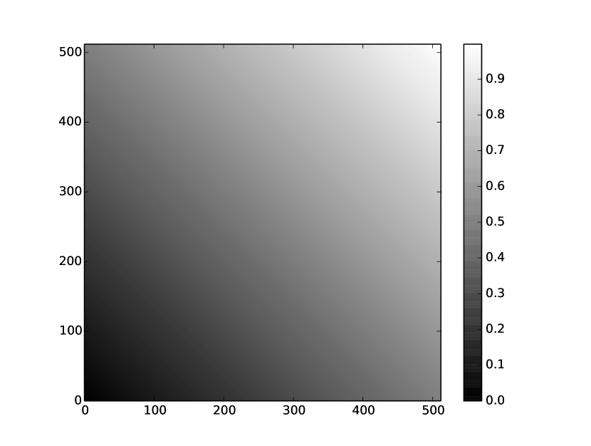
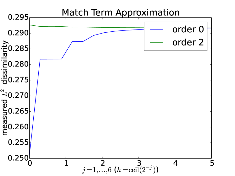
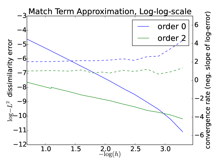
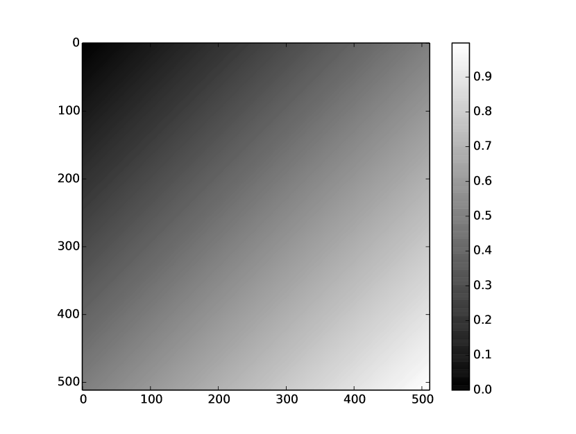
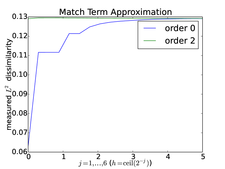
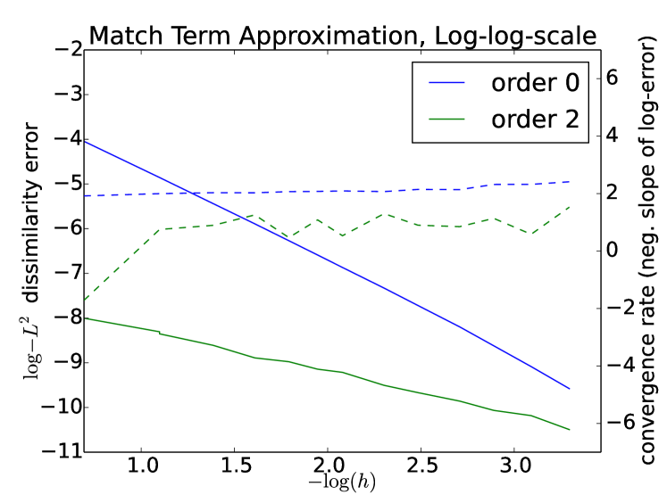
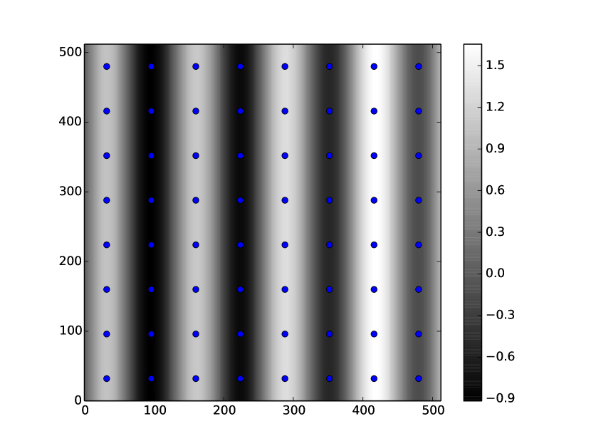
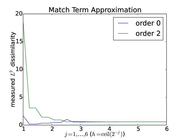
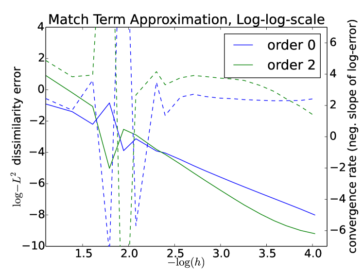
Figure 2: Convergence of matching functional Fh(k)superscriptsubscript𝐹𝑘F_{h}^{(k)}, k=0,2𝑘02k=0,2. Top row: (a) linear, (b) quadratic, and (c) non-polynomial images. Lower rows, horz. axis: decreasing hh (increasing nr. of sample points); vert. axis: Fh(k)superscriptsubscript𝐹𝑘F_{h}^{(k)} (solid, left axis) and convergence rate (dashed, right axis). With linear and quadratic images, the error is vanishing with k=2𝑘2k=2 and using only one sample point. Average convergence rates, k=0𝑘0k=0: quadratic; k=2𝑘2k=2: quartic as expected. (c, top row) sample points for h=23superscript23h=2^{-3} (23superscript232^{3} sample points per axis).

7.2 Jet Deformations

Figure 1 (page 1) shows the deformations encoded by zeroth, first and second order jet-particles on initially square grids. Note the locally affine deformations arising from the zeroth and first order jet-particles. Up to rotation of the axes, the three first order examples in the figure constitute a basis of the 4 dimensional space of first order jet-particles with fixed lower-order components. Likewise, up to rotation, the three second order examples constitute a basis for the 6 dimensional space of second order jet-particles.

7.3 Matching Functional Approximation

We here illustrate and test the convergence rate of the matching functional approximations. In Figure 2 (page 2), the approximations Fh(p)superscriptsubscript𝐹𝑝F_{h}^{(p)} are compared for p=0,2𝑝02p=0,2 and varying grid sizes on three synthetic images supported on the unit square. The first two images (a,b) are generated by first and second order polynomials, respectively, while the last image (c) is generated by a trigonometric function. A truncated Taylor expansion can therefore only approximate the image (c). The second order approximation Fh(2)superscriptsubscript𝐹2F_{h}^{(2)} models F𝐹F locally with a second order polynomial, and it is thus expected that the error should vanish on the images (a,b). As the mesh width hh decreases, we expect to observe O(h2)𝑂superscript2O(h^{2}) convergence rate for the zeroth order approximation Fh(0)superscriptsubscript𝐹0F_{h}^{(0)} on all three images. Likewise, we expect a convergence rate of O(h4)𝑂superscript4O(h^{4}) for Fh(2)superscriptsubscript𝐹2F_{h}^{(2)} on image (c).

In accordance with these expectations, we see the vanishing error for Fh(2)superscriptsubscript𝐹2F_{h}^{(2)} on (a,b) and decreasing error on (c) (lower row, solid green lines). The non-monotonic convergence seen on (c) is a result of the polynomial approximation being integrated over a compact domain. The zeroth order approximation Fh(0)superscriptsubscript𝐹0F_{h}^{(0)} likewise decreases with h2superscript2h^{2} convergence rate (lower row, dashed blue lines). The convergence rate of Fh(2)superscriptsubscript𝐹2F_{h}^{(2)} on image (c) stabilizes at approximately h4superscript4h^{4} until it decreases due to numerical errors introduced when the error approaches the machine precision.

Refer to caption
Refer to caption
Refer to caption
Refer to caption
Refer to caption
Refer to caption
Refer to caption
Refer to caption
Refer to caption
Refer to caption
Refer to caption
Refer to caption
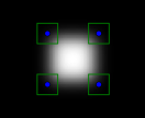
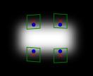
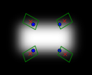
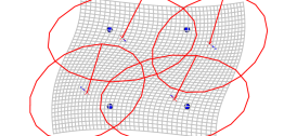
Figure 3: Matching moving images (b-d) to fixed image (a) using four jet-particles (blue points). Enlarged fixed image and moving images after warping (e-h). Corresponding deformations of an initially square grid (i-l). (b/f/j) Order 0; (c/g/k) order 1; (d/h/l) order 2. Red crosses mark location of jet-particles in moving images after matching, green boxes deformed by the warp Jacobian at the particle positions. Moving images at the red crosses should match fixed image at blue dots; second row images should match the fixed image (a/e).
Refer to caption
Refer to caption
Refer to caption
Refer to caption
Refer to caption
Refer to caption
Refer to caption
Refer to caption
Refer to caption
Refer to caption
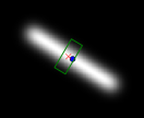
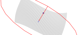
Figure 4: First order (linear/affine) deformations can be matched with multiple zeroth order jet-particles (a,b) or one first order jet-particle (c,d). A rotated bar (b/d) is matched to a bar (a/c). The warps that transform the moving images (b/d) to the fixed images (a/c) are applied to initially square grids (i/j) (rotated 90superscript9090^{\circ}). Red circles are deformed with warp derivative at the particle positions. (e-h) shows enlarged fixed and warped moving images. The amount of bending at the edges (f/h) is a function of the kernel size.

7.4 Matching Simple Structures

With the following set of examples, we wish to illustrate the effects of including second order information in the matching term approximation. We visualize this using simple test images. In all examples, we will employ the approximations Fh(k)superscriptsubscript𝐹𝑘F_{h}^{(k)} for k=0,2𝑘02k=0,2. In addition, we will match using only zeroth and first order information with a matching term that results from dropping the second order terms from Fh(2)superscriptsubscript𝐹2F_{h}^{(2)}. While this approximation does not arise naturally from a Taylor expansion of F𝐹F, it allows visualization of the differences between including first and second order image information in the match.

Refer to caption
Refer to caption
Refer to caption
Refer to caption
Refer to caption
Figure 5: Without higher order features, 2nd order jet-particles do not change the match: A blob (a) is translated and matched in moving images (b,d) with red crosses marking positions of jet-particles after match. Grids (c,e) illustrate the deformations that are equivalent for 0th order (b,c) and 2nd order (d,e).

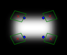
In Figure 3, a bar (moving image) is matched to a square (fixed image). The figure shows how four jet-particles move from their positions on a grid in the fixed image (a) to positions in the moving image that contain features matching the fixed image up to the order of the approximation. For zeroth order (b), only pointwise intensity is matched and the jet-particles move vertically (red crosses) resulting in only a slight deformation. With first order matching (c), the jet-particles locally rotate the domain (warp Jacobian matrices shown with green boxes) to account for the image gradient at the corners of the square. This produces a diamond-like shape. With second order (d), the corners are matched and the jet-particles move towards the corners of the moving image bar. The middle row shows the warped moving images enlarged. The second order match (h) is close to the fixed image (a) while both first and zeroth order fail to produce satisfying matches.

Refer to caption
(a) fixed, full image
Refer to caption
(b) fixed, region
Refer to caption
(c) moving, full image
Refer to caption
(d) mov., region
Refer to caption
(e) 2nd order, 9 jet-particles
Refer to caption
(f) 2nd order, 16 jet-particles
Refer to caption
(g) 2nd order, 64 jet-particles
Refer to caption
(h) 0th order, 9 jet-particles
Refer to caption
(i) 0th order, 16 jet-particles
Refer to caption
(j) 0th order, 64 jet-particles
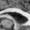
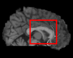
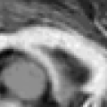
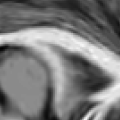
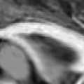
Figure 6: 2D registration of MRI slices, (a-b) fixed image, (c-d) moving image, red boxes: regions to be matched. Lower rows: matching results using 2nd order jet-particles (e-g), 0th order jet-particles (h-j). Images in lower rows should be close to (b). With 9 2nd order jet-particles (3 per axis), the moving image approaches the fixed. The match is visually good with 16 jet-particles (4 per axis). The ventricle region can equivalently be inflated with 64 0th order jet-particles.

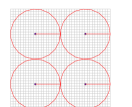
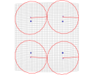
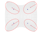
Figure 4 shows the result of matching images differing by an affine transformation with either one first order jet or multiple zeroth order jet-particles. While three zeroth order jet-particles can approximate a first order deformation in 2D, four particles are used to produce a symmetric picture. The warp Jacobians deform the initially square green boxes displayed at the jet positions. The resulting warps in both cases approximate an affine transformation.

With translation only, including second order information in the match does not change the result as illustrated in Figure 5 where the match is performed on an image and a translated version of the image.

7.5 Real image data

We illustrate the effect of the increased order on real images by matching two mid-sagittal slices of 3D MRI from the MGH10 dataset [KAA+09]. In Figure 6, red boxes mark the ventricle area of the brain on which the matching is performed. We perform the match with 9 jet-particles (3 per axis), 16 jet-particles (4 per axis) and 64 jet-particles (8 per axis) and k=0,2𝑘02k=0,2. With 9 second order jet-particles (e), the moving image (d) approaches the fixed (b). A visually good match is obtained with 16 or more jet-particles. 9 and 16 zeroth order jet-particles are not sufficient to correctly encode the expansion of the ventricle. With 64 zeroth order jet-particles, the transformed image is close to the results of the second order matches.

8 Conclusion and Future Work

A priori, the LDDMM framework of image registration poses an optimization problem on the space of diffeomorphism. Here, we introduced a family of discretized cost functions on a finite dimensional phase space that can be minimized numerically. The solutions of the discretized problem can be related to solutions of the full infinite-dimensional problem with O(hd+k)𝑂superscript𝑑𝑘O(h^{d+k}) accuracy, where hh is a grid spacing and k𝑘k is the order of approximation.

We provided numerical examples of deformations parametrized by zeroth, first, and second order jet-particles, and we showed examples of the higher order convergence of the similarity measure. The higher-order similarity measure allows matching of higher order features, and we use this fact to register various shapes and images with low numbers of jet-particles.

Representing a Cksuperscript𝐶𝑘C^{k} image requires much less information than representing a C0superscript𝐶0C^{0} image. Heuristically, the impact of this for computation is that we may use different techniques to approximate and advect smooth images with a sparse set of parameters. The higher-order accuracy schemes here constitutes a particular example of using reduction by symmetry to remove redundant information, and specialize advection to the data at hand. In this case, we reduce the dimensionality from infinite to finite for a given discretization, and we specialize the discretization to C2superscript𝐶2C^{2} images.

While the applicability of this specialization is limited to images of sufficient regularity, the bigger point of this article is the notion of tailoring discretizations to data. This approach is applicable for reducing the dimensionality of data beyond images. For example, accurate discretizations of curves with tangents, surfaces with tangent planes, and higher-order tensors can be derived with corresponding reduction in dimensionality. The present framework thus points to a general approach for higher-order accurate discretizations of general classes of matching problems. Future work will constitute testing these areas of wider applicability.

Acknowledgments

Henry O. Jacobs is supported by the European Research Council Advanced Grant 267382 FCCA. Stefan Sommer is supported by the Danish Council for Independent Research with the project “Image Based Quantification of Anatomical Change”. We would like to thank Klas Modin for summarizing the literature on analysis of the EPDiff equation, especially in regards to smoothness of initial conditions.

Appendix A Equations of motion

The equations of motion are expressible as Hamiltonian equations with respect to a non-canonical Poisson bracket. If we denote q(0)superscript𝑞0q^{(0)} simply by q𝑞q and p(0)superscript𝑝0p^{(0)} simply by p𝑝p then the Hamiltonian is

H(q,p,μ(1),μ(2))=𝐻𝑞𝑝superscript𝜇1superscript𝜇2absent\displaystyle H(q,p,\mu^{(1)},\mu^{(2)})= 12piαpjβKαβ(qiqj)piα[μj(1)]\indicesγβγKαβ(qiqj)12subscript𝑝𝑖𝛼subscript𝑝𝑗𝛽superscript𝐾𝛼𝛽subscript𝑞𝑖subscript𝑞𝑗subscript𝑝𝑖𝛼delimited-[]subscriptsuperscript𝜇1𝑗\indicessubscriptsuperscriptsubscript𝛾𝛾𝛽superscript𝐾𝛼𝛽subscript𝑞𝑖subscript𝑞𝑗\displaystyle\frac{1}{2}p_{i\alpha}p_{j\beta}K^{\alpha\beta}(q_{i}-q_{j})-p_{i\alpha}[\mu^{(1)}_{j}]\indices{{}_{\beta}^{\gamma}}\partial_{\gamma}K^{\alpha\beta}(q_{i}-q_{j}) (12)
+piα[μj(2)]\indicesδγβγδKαβ(qiqj)12[μi(1)]\indices[μj(1)]αδ\indicesδγβγKαβ(qiqj)\displaystyle+p_{i\alpha}[\mu^{(2)}_{j}]\indices{{}_{\beta}^{\gamma\delta}}\partial_{\delta\gamma}K^{\alpha\beta}(q_{i}-q_{j})-\frac{1}{2}[\mu_{i}^{(1)}]\indices{{}_{\alpha}^{\delta}}[\mu_{j}^{(1)}]\indices{{}_{\beta}^{\gamma}}\partial_{\delta\gamma}K^{\alpha\beta}(q_{i}-q_{j}) (13)
+[μi(1)]\indices[μj(2)]αϵ\indicesϵγδβγδKαβ(qiqj)\displaystyle+[\mu_{i}^{(1)}]\indices{{}_{\alpha}^{\epsilon}}[\mu_{j}^{(2)}]\indices{{}_{\beta}^{\gamma\delta}}\partial_{\epsilon\gamma\delta}K^{\alpha\beta}(q_{i}-q_{j}) (14)
+12[μi(2)]\indices[μj(2)]αϵϕ\indicesγδϵϕβγδKαβ(qiqj)\displaystyle+\frac{1}{2}[\mu_{i}^{(2)}]\indices{{}_{\alpha}^{\epsilon\phi}}[\mu_{j}^{(2)}]\indices{{}_{\beta}^{\gamma\delta}}\partial_{\gamma\delta\epsilon\phi}K^{\alpha\beta}(q_{i}-q_{j}) (15)

Where Kαβ(x)=δαβex2/2σ2superscript𝐾𝛼𝛽𝑥superscript𝛿𝛼𝛽superscript𝑒superscriptnorm𝑥22superscript𝜎2K^{\alpha\beta}(x)=\delta^{\alpha\beta}e^{-\|x\|^{2}/2\sigma^{2}}. Hamiton’s equations are then given in short by

q˙˙𝑞\displaystyle\dot{q} =Hpabsent𝐻𝑝\displaystyle=\frac{\partial H}{\partial p} (16)
p˙˙𝑝\displaystyle\dot{p} =Hqabsent𝐻𝑞\displaystyle=-\frac{\partial H}{\partial q} (17)
ξ𝜉\displaystyle\xi =Hμabsent𝐻𝜇\displaystyle=\frac{\partial H}{\partial\mu} (18)
μ˙˙𝜇\displaystyle\dot{\mu} =adξ(μ).absentsubscriptsuperscriptad𝜉𝜇\displaystyle=-\operatorname{ad}^{*}_{\xi}(\mu). (19)

More explicitly, equation (16) is given by

q˙iα=pjβKαβ(qiqj)[μj(1)]\indicesγβγKαβ(qiqj)+[μj(2)]\indicesγδβγδKαβ(qiqj)superscriptsubscript˙𝑞𝑖𝛼subscript𝑝𝑗𝛽superscript𝐾𝛼𝛽subscript𝑞𝑖subscript𝑞𝑗delimited-[]subscriptsuperscript𝜇1𝑗\indicessubscriptsuperscriptsubscript𝛾𝛾𝛽superscript𝐾𝛼𝛽subscript𝑞𝑖subscript𝑞𝑗delimited-[]subscriptsuperscript𝜇2𝑗\indicessubscriptsuperscriptsubscript𝛾𝛿𝛾𝛿𝛽superscript𝐾𝛼𝛽subscript𝑞𝑖subscript𝑞𝑗\displaystyle\dot{q}_{i}^{\alpha}=p_{j\beta}K^{\alpha\beta}(q_{i}-q_{j})-[\mu^{(1)}_{j}]\indices{{}_{\beta}^{\gamma}}\partial_{\gamma}K^{\alpha\beta}(q_{i}-q_{j})+[\mu^{(2)}_{j}]\indices{{}_{\beta}^{\gamma\delta}}\partial_{\gamma\delta}K^{\alpha\beta}(q_{i}-q_{j})

equation (17) is given by the sum

p˙iα=Tiα00+Tiα01+Tiα02+Tiα12+Tiα11+Tiα22subscript˙𝑝𝑖𝛼subscriptsuperscript𝑇00𝑖𝛼subscriptsuperscript𝑇01𝑖𝛼subscriptsuperscript𝑇02𝑖𝛼subscriptsuperscript𝑇12𝑖𝛼subscriptsuperscript𝑇11𝑖𝛼subscriptsuperscript𝑇22𝑖𝛼\displaystyle\dot{p}_{i\alpha}=T^{00}_{i\alpha}+T^{01}_{i\alpha}+T^{02}_{i\alpha}+T^{12}_{i\alpha}+T^{11}_{i\alpha}+T^{22}_{i\alpha}

Where we define the six terms in this sum as

Tiα00=subscriptsuperscript𝑇00𝑖𝛼absent\displaystyle T^{00}_{i\alpha}= piγpjβαKγβ(qiqj)subscript𝑝𝑖𝛾subscript𝑝𝑗𝛽subscript𝛼superscript𝐾𝛾𝛽subscript𝑞𝑖subscript𝑞𝑗\displaystyle-p_{i\gamma}p_{j\beta}\partial_{\alpha}K^{\gamma\beta}(q_{i}-q_{j})
Tiα01=subscriptsuperscript𝑇01𝑖𝛼absent\displaystyle T^{01}_{i\alpha}= (piδ[μj(1)]\indicesβγpjδ[μi(1)]\indices)βγγαKδβ(qiqj)\displaystyle(p_{i\delta}[\mu_{j}^{(1)}]\indices{{}_{\beta}^{\gamma}}-p_{j\delta}[\mu_{i}^{(1)}]\indices{{}_{\beta}^{\gamma}})\partial_{\gamma\alpha}K^{\delta\beta}(q_{i}-q_{j})
Tiα02=subscriptsuperscript𝑇02𝑖𝛼absent\displaystyle T^{02}_{i\alpha}= (piϵ[μj(2)]\indices+βγδpjϵ[μi(2)]\indices)βγδγδαKϵβ(qiqj)\displaystyle-(p_{i\epsilon}[\mu_{j}^{(2)}]\indices{{}_{\beta}^{\gamma\delta}}+p_{j\epsilon}[\mu_{i}^{(2)}]\indices{{}_{\beta}^{\gamma\delta}})\partial_{\gamma\delta\alpha}K^{\epsilon\beta}(q_{i}-q_{j})
Tiα12=subscriptsuperscript𝑇12𝑖𝛼absent\displaystyle T^{12}_{i\alpha}= ([μi(1)]\indices[μj(2)]ϕϵ\indicesβγδ[μj(1)]\indices[μi(2)]ϕϵ\indices)βγδϵγδαKϕβ(qiqj)\displaystyle-([\mu_{i}^{(1)}]\indices{{}_{\phi}^{\epsilon}}[\mu_{j}^{(2)}]\indices{{}_{\beta}^{\gamma\delta}}-[\mu_{j}^{(1)}]\indices{{}_{\phi}^{\epsilon}}[\mu_{i}^{(2)}]\indices{{}_{\beta}^{\gamma\delta}})\partial_{\epsilon\gamma\delta\alpha}K^{\phi\beta}(q_{i}-q_{j})
Tiα11=subscriptsuperscript𝑇11𝑖𝛼absent\displaystyle T^{11}_{i\alpha}= [μi(1)]\indices[μj(1)]ϵδ\indicesδγαβγKϵβ(qiqj)\displaystyle[\mu_{i}^{(1)}]\indices{{}_{\epsilon}^{\delta}}[\mu_{j}^{(1)}]\indices{{}_{\beta}^{\gamma}}\partial_{\delta\gamma\alpha}K^{\epsilon\beta}(q_{i}-q_{j})
Tiα22=subscriptsuperscript𝑇22𝑖𝛼absent\displaystyle T^{22}_{i\alpha}= [μi(2)]\indices[μj(2)]ζϵϕ\indicesϵδγϕαβγδKζβ(qiqj)\displaystyle-[\mu_{i}^{(2)}]\indices{{}_{\zeta}^{\epsilon\phi}}[\mu_{j}^{(2)}]\indices{{}_{\beta}^{\gamma\delta}}\partial_{\epsilon\delta\gamma\phi\alpha}K^{\zeta\beta}(q_{i}-q_{j})

Next, we calculate the quantities ξ(i)=H/μ(i)superscript𝜉𝑖𝐻superscript𝜇𝑖\xi^{(i)}=\partial H/\partial\mu^{(i)} for i=1,2𝑖12i=1,2 of equation (18) to be

[ξi(1)]\indices=βα\displaystyle[\xi_{i}^{(1)}]\indices{{}^{\alpha}_{\beta}}= pj,γβKαγ(qiqj)[μj(1)]\indicesβγδγKαδ(qiqj)+[μj(2)]\indicesβγδϵγδKαϵ(qiqj)subscript𝑝𝑗𝛾subscript𝛽superscript𝐾𝛼𝛾subscript𝑞𝑖subscript𝑞𝑗delimited-[]superscriptsubscript𝜇𝑗1\indicessubscriptsuperscriptsubscript𝛽𝛾𝛾𝛿superscript𝐾𝛼𝛿subscript𝑞𝑖subscript𝑞𝑗delimited-[]superscriptsubscript𝜇𝑗2\indicessubscriptsuperscriptsubscript𝛽𝛾𝛿𝛾𝛿italic-ϵsuperscript𝐾𝛼italic-ϵsubscript𝑞𝑖subscript𝑞𝑗\displaystyle p_{j,\gamma}\partial_{\beta}K^{\alpha\gamma}(q_{i}-q_{j})-[\mu_{j}^{(1)}]\indices{{}_{\delta}^{\gamma}}\partial_{\beta\gamma}K^{\alpha\delta}(q_{i}-q_{j})+[\mu_{j}^{(2)}]\indices{{}_{\epsilon}^{\gamma\delta}}\partial_{\beta\gamma\delta}K^{\alpha\epsilon}(q_{i}-q_{j})
[ξi(2)]\indices=βγα\displaystyle[\xi_{i}^{(2)}]\indices{{}^{\alpha}_{\beta\gamma}}= pjδβγKαδ(qiqj)[μj(1)]\indicesϵβγδϵKαδ(qiqj)+[μj(2)]\indicesβγϕδϵϕδKαϵ(qiqj)subscript𝑝𝑗𝛿subscript𝛽𝛾superscript𝐾𝛼𝛿subscript𝑞𝑖subscript𝑞𝑗delimited-[]superscriptsubscript𝜇𝑗1\indicessubscriptsuperscriptsubscriptitalic-ϵ𝛽𝛾italic-ϵ𝛿superscript𝐾𝛼𝛿subscript𝑞𝑖subscript𝑞𝑗delimited-[]superscriptsubscript𝜇𝑗2\indicessubscriptsuperscriptsubscript𝛽𝛾italic-ϕ𝛿italic-ϕ𝛿italic-ϵsuperscript𝐾𝛼italic-ϵsubscript𝑞𝑖subscript𝑞𝑗\displaystyle p_{j\delta}\partial_{\beta\gamma}K^{\alpha\delta}(q_{i}-q_{j})-[\mu_{j}^{(1)}]\indices{{}_{\delta}^{\epsilon}}\partial_{\epsilon\beta\gamma}K^{\alpha\delta}(q_{i}-q_{j})+[\mu_{j}^{(2)}]\indices{{}_{\epsilon}^{\phi\delta}}\partial_{\beta\gamma\phi\delta}K^{\alpha\epsilon}(q_{i}-q_{j})

which allows us to compute μ˙(i)superscript˙𝜇𝑖\dot{\mu}^{(i)} in equation (19) as

[μ˙i(1)]\indices=αβ\displaystyle[\dot{\mu}^{(1)}_{i}]\indices{{}_{\alpha}^{\beta}}= [μi(1)]\indices[ξi(1)]αγ\indicesγβ[μi(1)]\indices[ξi(1)]γβ\indicesαγ\displaystyle[\mu_{i}^{(1)}]\indices{{}_{\alpha}^{\gamma}}[\xi_{i}^{(1)}]\indices{{}^{\beta}_{\gamma}}-[\mu_{i}^{(1)}]\indices{{}_{\gamma}^{\beta}}[\xi_{i}^{(1)}]\indices{{}^{\gamma}_{\alpha}}
+[μi(2)]\indices[ξi(2)]αδγ\indicesδγβ[μi(2)]\indices[ξi(2)]δβγ\indicesαγδ[μi(2)]\indices[ξi(2)]δγβ\indicesγαδ\displaystyle+[\mu_{i}^{(2)}]\indices{{}_{\alpha}^{\delta\gamma}}[\xi_{i}^{(2)}]\indices{{}^{\beta}_{\delta\gamma}}-[\mu_{i}^{(2)}]\indices{{}_{\delta}^{\beta\gamma}}[\xi_{i}^{(2)}]\indices{{}^{\delta}_{\alpha\gamma}}-[\mu_{i}^{(2)}]\indices{{}_{\delta}^{\gamma\beta}}[\xi_{i}^{(2)}]\indices{{}^{\delta}_{\gamma\alpha}}
[μi˙(2)]\indices=αβγ\displaystyle[\dot{\mu_{i}}^{(2)}]\indices{{}_{\alpha}^{\beta\gamma}}= [μi(2)]\indices[ξi(1)]αδγ\indices+δβ[μi(2)]\indices[ξi(1)]αβδ\indicesδγ[μi(2)]\indices[ξi(1)]δβγ\indicesαδ\displaystyle[\mu_{i}^{(2)}]\indices{{}_{\alpha}^{\delta\gamma}}[\xi_{i}^{(1)}]\indices{{}^{\beta}_{\delta}}+[\mu_{i}^{(2)}]\indices{{}_{\alpha}^{\beta\delta}}[\xi_{i}^{(1)}]\indices{{}^{\gamma}_{\delta}}-[\mu_{i}^{(2)}]\indices{{}_{\delta}^{\beta\gamma}}[\xi_{i}^{(1)}]\indices{{}^{\delta}_{\alpha}}

A.1 Computing q˙˙𝑞\dot{q} as a function of ξ𝜉\xi

The action of ξ𝜉\xi on q𝑞q is given by ξq𝜉𝑞\xi\cdot q. We set q˙=ξq˙𝑞𝜉𝑞\dot{q}=\xi\cdot q. We’ve already calculated q˙(0)superscript˙𝑞0\dot{q}^{(0)}. We need only calculate q˙(1)superscript˙𝑞1\dot{q}^{(1)} and q˙(2)superscript˙𝑞2\dot{q}^{(2)}. Componentwise we calculate these to be

[q˙(1)]\indices=βα\displaystyle[\dot{q}^{(1)}]\indices{{}^{\alpha}_{\beta}}= [ξ(1)]\indices[q(1)]γα\indicesβγ\displaystyle[\xi^{(1)}]\indices{{}^{\alpha}_{\gamma}}[q^{(1)}]\indices{{}^{\gamma}_{\beta}}
[q˙(2)]\indices=βγα\displaystyle[\dot{q}^{(2)}]\indices{{}^{\alpha}_{\beta\gamma}}= [ξ(2)]\indicesδϵα[q(1)]\indicesβδ[q(1)]\indices+γϵ[ξ(1)]\indicesδα[q(2)]\indicesβγδ\displaystyle[\xi^{(2)}]\indices{{}^{\alpha}_{\delta\epsilon}}\cdot[q^{(1)}]\indices{{}^{\delta}_{\beta}}\cdot[q^{(1)}]\indices{{}^{\epsilon}_{\gamma}}+[\xi^{(1)}]\indices{{}^{\alpha}_{\delta}}\cdot[q^{(2)}]\indices{{}^{\delta}_{\beta\gamma}}

Appendix B First variation equations

The first variation equations are equivalent to applying the tangent functor to our evolutions. We find the velocites:

ddtδqiα=𝑑𝑑𝑡𝛿superscriptsubscript𝑞𝑖𝛼absent\displaystyle\frac{d}{dt}\delta q_{i}^{\alpha}= δpjβKαβ(qiqj)+pjβ(δqiγδqjγ)γKαβ(qiqj)𝛿subscript𝑝𝑗𝛽superscript𝐾𝛼𝛽subscript𝑞𝑖subscript𝑞𝑗subscript𝑝𝑗𝛽𝛿superscriptsubscript𝑞𝑖𝛾𝛿superscriptsubscript𝑞𝑗𝛾subscript𝛾superscript𝐾𝛼𝛽subscript𝑞𝑖subscript𝑞𝑗\displaystyle\delta p_{j\beta}K^{\alpha\beta}(q_{i}-q_{j})+p_{j\beta}(\delta q_{i}^{\gamma}-\delta q_{j}^{\gamma})\partial_{\gamma}K^{\alpha\beta}(q_{i}-q_{j})
[δμj(1)]\indicesγβγKαβ(qiqj)[μj(1)]\indicesγδβγKαβ(qiqj)(δqiδδqjδ)delimited-[]𝛿superscriptsubscript𝜇𝑗1\indicessubscriptsuperscriptsubscript𝛾𝛾𝛽superscript𝐾𝛼𝛽subscript𝑞𝑖subscript𝑞𝑗delimited-[]superscriptsubscript𝜇𝑗1\indicessubscriptsuperscriptsubscript𝛾𝛿𝛾𝛽superscript𝐾𝛼𝛽subscript𝑞𝑖subscript𝑞𝑗𝛿superscriptsubscript𝑞𝑖𝛿𝛿superscriptsubscript𝑞𝑗𝛿\displaystyle-[\delta\mu_{j}^{(1)}]\indices{{}_{\beta}^{\gamma}}\partial_{\gamma}K^{\alpha\beta}(q_{i}-q_{j})-[\mu_{j}^{(1)}]\indices{{}_{\beta}^{\gamma}}\partial_{\gamma\delta}K^{\alpha\beta}(q_{i}-q_{j})(\delta q_{i}^{\delta}-\delta q_{j}^{\delta})
+[δμj(2)]\indicesγδβγδKαβ(qiqj)+[μj(2)]\indicesγδϵβγδKαβ(qiqj)(δqiϵδqjϵ)delimited-[]𝛿superscriptsubscript𝜇𝑗2\indicessubscriptsuperscriptsubscript𝛾𝛿𝛾𝛿𝛽superscript𝐾𝛼𝛽subscript𝑞𝑖subscript𝑞𝑗delimited-[]superscriptsubscript𝜇𝑗2\indicessubscriptsuperscriptsubscript𝛾𝛿italic-ϵ𝛾𝛿𝛽superscript𝐾𝛼𝛽subscript𝑞𝑖subscript𝑞𝑗𝛿superscriptsubscript𝑞𝑖italic-ϵ𝛿superscriptsubscript𝑞𝑗italic-ϵ\displaystyle+[\delta\mu_{j}^{(2)}]\indices{{}_{\beta}^{\gamma\delta}}\partial_{\gamma\delta}K^{\alpha\beta}(q_{i}-q_{j})+[\mu_{j}^{(2)}]\indices{{}_{\beta}^{\gamma\delta}}\partial_{\gamma\delta\epsilon}K^{\alpha\beta}(q_{i}-q_{j})(\delta q_{i}^{\epsilon}-\delta q_{j}^{\epsilon})
[δξi(1)]\indices=βα\displaystyle[\delta\xi^{(1)}_{i}]\indices{{}^{\alpha}_{\beta}}= δpjγβKγα(qiqj)+pjγ(δqiδδqjδ)δβKαγ(qiqj)𝛿subscript𝑝𝑗𝛾subscript𝛽superscript𝐾𝛾𝛼subscript𝑞𝑖subscript𝑞𝑗subscript𝑝𝑗𝛾𝛿superscriptsubscript𝑞𝑖𝛿𝛿superscriptsubscript𝑞𝑗𝛿subscript𝛿𝛽superscript𝐾𝛼𝛾subscript𝑞𝑖subscript𝑞𝑗\displaystyle\delta p_{j\gamma}\partial_{\beta}K^{\gamma\alpha}(q_{i}-q_{j})+p_{j\gamma}(\delta q_{i}^{\delta}-\delta q_{j}^{\delta})\partial_{\delta\beta}K^{\alpha\gamma}(q_{i}-q_{j})
[δμj(1)]\indicesβγδγKαδ(qiqj)[μj(1)]\indices(δqiϵδqjϵ)δγβγϵKαδ(qiqj)\displaystyle-[\delta\mu_{j}^{(1)}]\indices{{}_{\delta}^{\gamma}}\partial_{\beta\gamma}K^{\alpha\delta}(q_{i}-q_{j})-[\mu_{j}^{(1)}]\indices{{}_{\delta}^{\gamma}}(\delta q_{i}^{\epsilon}-\delta q_{j}^{\epsilon})\partial_{\beta\gamma\epsilon}K^{\alpha\delta}(q_{i}-q_{j})
+[δμj(2)]\indicesβγδϕγδKαϕ(qiqj)+[μj(2)]\indices(δqiϵδqjϵ)ϕγδβγδϵKαϕ(qiqj)\displaystyle+[\delta\mu_{j}^{(2)}]\indices{{}_{\phi}^{\gamma\delta}}\partial_{\beta\gamma\delta}K^{\alpha\phi}(q_{i}-q_{j})+[\mu_{j}^{(2)}]\indices{{}_{\phi}^{\gamma\delta}}(\delta q_{i}^{\epsilon}-\delta q_{j}^{\epsilon})\partial_{\beta\gamma\delta\epsilon}K^{\alpha\phi}(q_{i}-q_{j})
[δξi(2)]\indices=βγα\displaystyle[\delta\xi^{(2)}_{i}]\indices{{}^{\alpha}_{\beta\gamma}}= δpjδβγKαδ(ij)+pjϵ(δqiδδqjδ)βγδKαϵ(ij)𝛿subscript𝑝𝑗𝛿subscript𝛽𝛾superscript𝐾𝛼𝛿𝑖𝑗subscript𝑝𝑗italic-ϵ𝛿superscriptsubscript𝑞𝑖𝛿𝛿superscriptsubscript𝑞𝑗𝛿subscript𝛽𝛾𝛿superscript𝐾𝛼italic-ϵ𝑖𝑗\displaystyle\delta p_{j\delta}\partial_{\beta\gamma}K^{\alpha\delta}(ij)+p_{j\epsilon}(\delta q_{i}^{\delta}-\delta q_{j}^{\delta})\partial_{\beta\gamma\delta}K^{\alpha\epsilon}(ij)
[δμj(1)]\indicesβγδϵδKαϵ(ij)[μj(1)]\indices(δqiϵδqjϵ)ϕδβγδϵKαϕ(ij)\displaystyle-[\delta\mu_{j}^{(1)}]\indices{{}_{\epsilon}^{\delta}}\partial_{\beta\gamma\delta}K^{\alpha\epsilon}(ij)-[\mu_{j}^{(1)}]\indices{{}_{\phi}^{\delta}}(\delta q_{i}^{\epsilon}-\delta q_{j}^{\epsilon})\partial_{\beta\gamma\delta\epsilon}K^{\alpha\phi}(ij)
+[δμj(2)]\indicesβγδϵϕδϵKαϕ(ij)+[μj(2)]\indices(δqiϕδqjϕ)λδϵβγδϵϕKαλ(ij)\displaystyle+[\delta\mu_{j}^{(2)}]\indices{{}_{\phi}^{\delta\epsilon}}\partial_{\beta\gamma\delta\epsilon}K^{\alpha\phi}(ij)+[\mu_{j}^{(2)}]\indices{{}_{\lambda}^{\delta\epsilon}}(\delta q_{i}^{\phi}-\delta q_{j}^{\phi})\partial_{\beta\gamma\delta\epsilon\phi}K^{\alpha\lambda}(ij)

and the momenta:

ddtδpiα=𝑑𝑑𝑡𝛿subscript𝑝𝑖𝛼absent\displaystyle\frac{d}{dt}\delta p_{i\alpha}= δTiα00+δTiα01+δTiα02+δTiα12+δTiα11+δTiα22𝛿subscriptsuperscript𝑇00𝑖𝛼𝛿subscriptsuperscript𝑇01𝑖𝛼𝛿subscriptsuperscript𝑇02𝑖𝛼𝛿subscriptsuperscript𝑇12𝑖𝛼𝛿subscriptsuperscript𝑇11𝑖𝛼𝛿subscriptsuperscript𝑇22𝑖𝛼\displaystyle\delta T^{00}_{i\alpha}+\delta T^{01}_{i\alpha}+\delta T^{02}_{i\alpha}+\delta T^{12}_{i\alpha}+\delta T^{11}_{i\alpha}+\delta T^{22}_{i\alpha}

The first-variation equation for μ(1)superscript𝜇1\mu^{(1)} is

ddt[δμ(1)]\indices=αβ\displaystyle\frac{d}{dt}[\delta\mu^{(1)}]\indices{{}_{\alpha}^{\beta}}= [δμ(1)]\indices[ξ(1)]αγ\indices+γβ[μ(1)]\indices[δξ(1)]αγ\indicesγβ\displaystyle[\delta\mu^{(1)}]\indices{{}_{\alpha}^{\gamma}}[\xi^{(1)}]\indices{{}^{\beta}_{\gamma}}+[\mu^{(1)}]\indices{{}_{\alpha}^{\gamma}}[\delta\xi^{(1)}]\indices{{}^{\beta}_{\gamma}}
[δμ(1)]\indices[ξ(1)]γβ\indicesαγ[μ(1)]\indices[δξ(1)]γβ\indicesαγ\displaystyle-[\delta\mu^{(1)}]\indices{{}_{\gamma}^{\beta}}[\xi^{(1)}]\indices{{}^{\gamma}_{\alpha}}-[\mu^{(1)}]\indices{{}_{\gamma}^{\beta}}[\delta\xi^{(1)}]\indices{{}^{\gamma}_{\alpha}}
+[δμ(2)]\indices[ξ(2)]αδγ\indices+δγβ[μ(2)]\indices[δξ(2)]αδγ\indicesδγβ\displaystyle+[\delta\mu^{(2)}]\indices{{}_{\alpha}^{\delta\gamma}}[\xi^{(2)}]\indices{{}^{\beta}_{\delta\gamma}}+[\mu^{(2)}]\indices{{}_{\alpha}^{\delta\gamma}}[\delta\xi^{(2)}]\indices{{}^{\beta}_{\delta\gamma}}
[δμ(2)]\indices[ξ(2)]δβγ\indicesαγδ[μ(2)]\indices[δξ(2)]δβγ\indicesαγδ\displaystyle-[\delta\mu^{(2)}]\indices{{}_{\delta}^{\beta\gamma}}[\xi^{(2)}]\indices{{}^{\delta}_{\alpha\gamma}}-[\mu^{(2)}]\indices{{}_{\delta}^{\beta\gamma}}[\delta\xi^{(2)}]\indices{{}^{\delta}_{\alpha\gamma}}
[δμ(2)]\indices[ξ(2)]δγβ\indicesγαδ[μ(2)]\indices[δξ(2)]δγβ\indicesγαδ\displaystyle-[\delta\mu^{(2)}]\indices{{}_{\delta}^{\gamma\beta}}[\xi^{(2)}]\indices{{}^{\delta}_{\gamma\alpha}}-[\mu^{(2)}]\indices{{}_{\delta}^{\gamma\beta}}[\delta\xi^{(2)}]\indices{{}^{\delta}_{\gamma\alpha}}

and finally

ddt[δμ(2)]\indices=αβγ\displaystyle\frac{d}{dt}[\delta\mu^{(2)}]\indices{{}_{\alpha}^{\beta\gamma}}= [δμ(2)]\indices[ξ(1)]αδγ\indices+δβ[μ(2)]\indices[δξ(1)]αδγ\indicesδβ\displaystyle[\delta\mu^{(2)}]\indices{{}_{\alpha}^{\delta\gamma}}[\xi^{(1)}]\indices{{}^{\beta}_{\delta}}+[\mu^{(2)}]\indices{{}_{\alpha}^{\delta\gamma}}[\delta\xi^{(1)}]\indices{{}^{\beta}_{\delta}}
+[δμ(2)]\indices[ξ(1)]αβδ\indices+δγ[μ(2)]\indices[δξ(1)]αβδ\indicesδγ\displaystyle+[\delta\mu^{(2)}]\indices{{}_{\alpha}^{\beta\delta}}[\xi^{(1)}]\indices{{}^{\gamma}_{\delta}}+[\mu^{(2)}]\indices{{}_{\alpha}^{\beta\delta}}[\delta\xi^{(1)}]\indices{{}^{\gamma}_{\delta}}
[δμ(2)]\indices[ξ(1)]δβγ\indicesαδ[μ(2)]\indices[δξ(1)]δβγ\indicesαδ\displaystyle-[\delta\mu^{(2)}]\indices{{}_{\delta}^{\beta\gamma}}[\xi^{(1)}]\indices{{}^{\delta}_{\alpha}}-[\mu^{(2)}]\indices{{}_{\delta}^{\beta\gamma}}[\delta\xi^{(1)}]\indices{{}^{\delta}_{\alpha}}

where the δT𝛿𝑇\delta T’s are given by

δTiα00=𝛿subscriptsuperscript𝑇00𝑖𝛼absent\displaystyle\delta T^{00}_{i\alpha}= δpiγpjβαKγβ(qiqj)piγδpjβαKγβ(qiqj)𝛿subscript𝑝𝑖𝛾subscript𝑝𝑗𝛽subscript𝛼superscript𝐾𝛾𝛽subscript𝑞𝑖subscript𝑞𝑗subscript𝑝𝑖𝛾𝛿subscript𝑝𝑗𝛽subscript𝛼superscript𝐾𝛾𝛽subscript𝑞𝑖subscript𝑞𝑗\displaystyle-\delta p_{i\gamma}p_{j\beta}\partial_{\alpha}K^{\gamma\beta}(q_{i}-q_{j})-p_{i\gamma}\delta p_{j\beta}\partial_{\alpha}K^{\gamma\beta}(q_{i}-q_{j})
piγpjβαδKγβ(qiqj)(δqiδδqjδ)subscript𝑝𝑖𝛾subscript𝑝𝑗𝛽subscript𝛼𝛿superscript𝐾𝛾𝛽subscript𝑞𝑖subscript𝑞𝑗𝛿superscriptsubscript𝑞𝑖𝛿𝛿superscriptsubscript𝑞𝑗𝛿\displaystyle-p_{i\gamma}p_{j\beta}\partial_{\alpha\delta}K^{\gamma\beta}(q_{i}-q_{j})(\delta q_{i}^{\delta}-\delta q_{j}^{\delta})
δTiα01=𝛿subscriptsuperscript𝑇01𝑖𝛼absent\displaystyle\delta T^{01}_{i\alpha}= δpjδ[μi(1)]\indicesγαβγKδβ(ij)pjδ[δμi(1)]\indicesγαβγKδβ(ij)𝛿subscript𝑝𝑗𝛿delimited-[]superscriptsubscript𝜇𝑖1\indicessubscriptsuperscriptsubscript𝛾𝛼𝛾𝛽superscript𝐾𝛿𝛽𝑖𝑗subscript𝑝𝑗𝛿delimited-[]𝛿superscriptsubscript𝜇𝑖1\indicessubscriptsuperscriptsubscript𝛾𝛼𝛾𝛽superscript𝐾𝛿𝛽𝑖𝑗\displaystyle-\delta p_{j\delta}[\mu_{i}^{(1)}]\indices{{}_{\beta}^{\gamma}}\partial_{\gamma\alpha}K^{\delta\beta}(ij)-p_{j\delta}[\delta\mu_{i}^{(1)}]\indices{{}_{\beta}^{\gamma}}\partial_{\gamma\alpha}K^{\delta\beta}(ij)
pjδ[μi(1)]\indices(δqiϵδqjϵ)βγϵγαKδβ(ij)\displaystyle-p_{j\delta}[\mu_{i}^{(1)}]\indices{{}_{\beta}^{\gamma}}(\delta q_{i}^{\epsilon}-\delta q_{j}^{\epsilon})\partial_{\epsilon\gamma\alpha}K^{\delta\beta}(ij)
+δpiδ[μj(1)]\indicesγαβγKδβ(ij)+piδ[δμj(1)]\indicesγαβγKδβ(ij)𝛿subscript𝑝𝑖𝛿delimited-[]superscriptsubscript𝜇𝑗1\indicessubscriptsuperscriptsubscript𝛾𝛼𝛾𝛽superscript𝐾𝛿𝛽𝑖𝑗subscript𝑝𝑖𝛿delimited-[]𝛿superscriptsubscript𝜇𝑗1\indicessubscriptsuperscriptsubscript𝛾𝛼𝛾𝛽superscript𝐾𝛿𝛽𝑖𝑗\displaystyle+\delta p_{i\delta}[\mu_{j}^{(1)}]\indices{{}_{\beta}^{\gamma}}\partial_{\gamma\alpha}K^{\delta\beta}(ij)+p_{i\delta}[\delta\mu_{j}^{(1)}]\indices{{}_{\beta}^{\gamma}}\partial_{\gamma\alpha}K^{\delta\beta}(ij)
+piδ[μj(1)]\indices(δqiϵδqjϵ)βγϵγαKδβ(ij)\displaystyle+p_{i\delta}[\mu_{j}^{(1)}]\indices{{}_{\beta}^{\gamma}}(\delta q_{i}^{\epsilon}-\delta q_{j}^{\epsilon})\partial_{\epsilon\gamma\alpha}K^{\delta\beta}(ij)
δTiα02=𝛿subscriptsuperscript𝑇02𝑖𝛼absent\displaystyle\delta T^{02}_{i\alpha}= δpiϵ[μj(2)]\indicesγδαβγδKϵβ(ij)piϵ[δμj(2)]\indicesγδαβγδKϵβ(ij)𝛿subscript𝑝𝑖italic-ϵdelimited-[]superscriptsubscript𝜇𝑗2\indicessubscriptsuperscriptsubscript𝛾𝛿𝛼𝛾𝛿𝛽superscript𝐾italic-ϵ𝛽𝑖𝑗subscript𝑝𝑖italic-ϵdelimited-[]𝛿superscriptsubscript𝜇𝑗2\indicessubscriptsuperscriptsubscript𝛾𝛿𝛼𝛾𝛿𝛽superscript𝐾italic-ϵ𝛽𝑖𝑗\displaystyle-\delta p_{i\epsilon}[\mu_{j}^{(2)}]\indices{{}_{\beta}^{\gamma\delta}}\partial_{\gamma\delta\alpha}K^{\epsilon\beta}(ij)-p_{i\epsilon}[\delta\mu_{j}^{(2)}]\indices{{}_{\beta}^{\gamma\delta}}\partial_{\gamma\delta\alpha}K^{\epsilon\beta}(ij)
piϵ[μj(2)]\indices(δqiϕδqjϕ)βγδγδϕαKϵβ(ij)\displaystyle-p_{i\epsilon}[\mu_{j}^{(2)}]\indices{{}_{\beta}^{\gamma\delta}}(\delta q_{i}^{\phi}-\delta q_{j}^{\phi})\partial_{\gamma\delta\phi\alpha}K^{\epsilon\beta}(ij)
δpjϵ[μi(2)]\indicesγδαβγδKϵβ(ij)pjϵ[δμi(2)]\indicesγδαβγδKϵβ(ij)𝛿subscript𝑝𝑗italic-ϵdelimited-[]superscriptsubscript𝜇𝑖2\indicessubscriptsuperscriptsubscript𝛾𝛿𝛼𝛾𝛿𝛽superscript𝐾italic-ϵ𝛽𝑖𝑗subscript𝑝𝑗italic-ϵdelimited-[]𝛿superscriptsubscript𝜇𝑖2\indicessubscriptsuperscriptsubscript𝛾𝛿𝛼𝛾𝛿𝛽superscript𝐾italic-ϵ𝛽𝑖𝑗\displaystyle-\delta p_{j\epsilon}[\mu_{i}^{(2)}]\indices{{}_{\beta}^{\gamma\delta}}\partial_{\gamma\delta\alpha}K^{\epsilon\beta}(ij)-p_{j\epsilon}[\delta\mu_{i}^{(2)}]\indices{{}_{\beta}^{\gamma\delta}}\partial_{\gamma\delta\alpha}K^{\epsilon\beta}(ij)
pjϵ[μi(2)]\indices(δqiϕδqjϕ)βγδγδϕαKϵβ(ij)\displaystyle-p_{j\epsilon}[\mu_{i}^{(2)}]\indices{{}_{\beta}^{\gamma\delta}}(\delta q_{i}^{\phi}-\delta q_{j}^{\phi})\partial_{\gamma\delta\phi\alpha}K^{\epsilon\beta}(ij)
δTiα12=𝛿subscriptsuperscript𝑇12𝑖𝛼absent\displaystyle\delta T^{12}_{i\alpha}= [δμi(1)]\indices[μj(2)]ϕϵ\indicesϵγδαβγδKϕβ(ij)\displaystyle-[\delta\mu_{i}^{(1)}]\indices{{}_{\phi}^{\epsilon}}[\mu_{j}^{(2)}]\indices{{}_{\beta}^{\gamma\delta}}\partial_{\epsilon\gamma\delta\alpha}K^{\phi\beta}(ij)
[μi(1)]\indices[δμj(2)]ϕϵ\indicesϵγδαβγδKϕβ(ij)\displaystyle-[\mu_{i}^{(1)}]\indices{{}_{\phi}^{\epsilon}}[\delta\mu_{j}^{(2)}]\indices{{}_{\beta}^{\gamma\delta}}\partial_{\epsilon\gamma\delta\alpha}K^{\phi\beta}(ij)
[μi(1)]\indices[μj(2)]ϕϵ\indices(δqiζδqjζ)βγδζϵγδαKϕβ(ij)\displaystyle-[\mu_{i}^{(1)}]\indices{{}_{\phi}^{\epsilon}}[\mu_{j}^{(2)}]\indices{{}_{\beta}^{\gamma\delta}}(\delta q_{i}^{\zeta}-\delta q_{j}^{\zeta})\partial_{\zeta\epsilon\gamma\delta\alpha}K^{\phi\beta}(ij)
+[δμj(1)]\indices[μi(2)]ϕϵ\indicesϵγδαβγδKϕβ(ij)\displaystyle+[\delta\mu_{j}^{(1)}]\indices{{}_{\phi}^{\epsilon}}[\mu_{i}^{(2)}]\indices{{}_{\beta}^{\gamma\delta}}\partial_{\epsilon\gamma\delta\alpha}K^{\phi\beta}(ij)
+[μj(1)]\indices[δμi(2)]ϕϵ\indicesϵγδαβγδKϕβ(ij)\displaystyle+[\mu_{j}^{(1)}]\indices{{}_{\phi}^{\epsilon}}[\delta\mu_{i}^{(2)}]\indices{{}_{\beta}^{\gamma\delta}}\partial_{\epsilon\gamma\delta\alpha}K^{\phi\beta}(ij)
+[μj(1)]\indices[μi(2)]ϕϵ\indices(δqiζδqjζ)βγδζϵγδαKϕβ(ij)\displaystyle+[\mu_{j}^{(1)}]\indices{{}_{\phi}^{\epsilon}}[\mu_{i}^{(2)}]\indices{{}_{\beta}^{\gamma\delta}}(\delta q_{i}^{\zeta}-\delta q_{j}^{\zeta})\partial_{\zeta\epsilon\gamma\delta\alpha}K^{\phi\beta}(ij)
δTiα11=𝛿subscriptsuperscript𝑇11𝑖𝛼absent\displaystyle\delta T^{11}_{i\alpha}= ([δμi(1)]\indices[μj(1)]ϵδ\indices+βγ[μi(1)]\indices[δμj(1)]ϵδ\indices)βγδγαKϵβ(ij)\displaystyle([\delta\mu_{i}^{(1)}]\indices{{}_{\epsilon}^{\delta}}[\mu_{j}^{(1)}]\indices{{}_{\beta}^{\gamma}}+[\mu_{i}^{(1)}]\indices{{}_{\epsilon}^{\delta}}[\delta\mu_{j}^{(1)}]\indices{{}_{\beta}^{\gamma}})\partial_{\delta\gamma\alpha}K^{\epsilon\beta}(ij)
+[μi(1)]\indices[μj(1)]ϵδ\indices(δqiϕδqjϕ)βγϕδγαKϵβ(ij)\displaystyle+[\mu_{i}^{(1)}]\indices{{}_{\epsilon}^{\delta}}[\mu_{j}^{(1)}]\indices{{}_{\beta}^{\gamma}}(\delta q_{i}^{\phi}-\delta q_{j}^{\phi})\partial_{\phi\delta\gamma\alpha}K^{\epsilon\beta}(ij)
δTiα22=𝛿subscriptsuperscript𝑇22𝑖𝛼absent\displaystyle\delta T^{22}_{i\alpha}= ([δμi(2)]\indices[μj(2)]ζϵϕ\indices+βγδ[μi(2)]\indices[δμj(2)]ζϵϕ\indices)βγδϵδγϕαKζβ(ij)\displaystyle-([\delta\mu_{i}^{(2)}]\indices{{}_{\zeta}^{\epsilon\phi}}[\mu_{j}^{(2)}]\indices{{}_{\beta}^{\gamma\delta}}+[\mu_{i}^{(2)}]\indices{{}_{\zeta}^{\epsilon\phi}}[\delta\mu_{j}^{(2)}]\indices{{}_{\beta}^{\gamma\delta}})\partial_{\epsilon\delta\gamma\phi\alpha}K^{\zeta\beta}(ij)
[μi(2)]\indices[μj(2)]ζϵϕ\indices(δqiλδqjλ)βγδλϵδγϕαKζβ(ij)\displaystyle-[\mu_{i}^{(2)}]\indices{{}_{\zeta}^{\epsilon\phi}}[\mu_{j}^{(2)}]\indices{{}_{\beta}^{\gamma\delta}}(\delta q_{i}^{\lambda}-\delta q_{j}^{\lambda})\partial_{\lambda\epsilon\delta\gamma\phi\alpha}K^{\zeta\beta}(ij)

Finally, we compute the variation equations for δq(1)𝛿superscript𝑞1\delta q^{(1)} and δq(2)𝛿superscript𝑞2\delta q^{(2)} to be

δ[q˙i(1)]\indices=βα\displaystyle\delta[\dot{q}_{i}^{(1)}]\indices{{}^{\alpha}_{\beta}}= [δξi(1)]\indices[qi(1)]γα\indices+βγ[ξi(1)]\indices[δqi(1)]γα\indicesβγ\displaystyle[\delta\xi_{i}^{(1)}]\indices{{}^{\alpha}_{\gamma}}[q_{i}^{(1)}]\indices{{}^{\gamma}_{\beta}}+[\xi_{i}^{(1)}]\indices{{}^{\alpha}_{\gamma}}[\delta q_{i}^{(1)}]\indices{{}^{\gamma}_{\beta}}
δ[q˙(2)]\indices=βγα\displaystyle\delta[\dot{q}^{(2)}]\indices{{}^{\alpha}_{\beta\gamma}}= [δξ(2)]\indicesδϵα[q(1)]\indicesβδ[q(1)]\indices+γϵ[ξ(2)]\indicesδϵα[δq(1)]\indicesβδ[q(1)]\indicesγϵ\displaystyle[\delta\xi^{(2)}]\indices{{}^{\alpha}_{\delta\epsilon}}\cdot[q^{(1)}]\indices{{}^{\delta}_{\beta}}\cdot[q^{(1)}]\indices{{}^{\epsilon}_{\gamma}}+[\xi^{(2)}]\indices{{}^{\alpha}_{\delta\epsilon}}\cdot[\delta q^{(1)}]\indices{{}^{\delta}_{\beta}}\cdot[q^{(1)}]\indices{{}^{\epsilon}_{\gamma}}
+[ξ(2)]\indicesδϵα[q(1)]\indicesβδ[δq(1)]\indices+γϵ[δξ(1)]\indicesδα[q(2)]\indices+βγδ[ξ(1)]\indicesδα[δq(2)]\indicesβγδ\displaystyle+[\xi^{(2)}]\indices{{}^{\alpha}_{\delta\epsilon}}\cdot[q^{(1)}]\indices{{}^{\delta}_{\beta}}\cdot[\delta q^{(1)}]\indices{{}^{\epsilon}_{\gamma}}+[\delta\xi^{(1)}]\indices{{}^{\alpha}_{\delta}}\cdot[q^{(2)}]\indices{{}^{\delta}_{\beta\gamma}}+[\xi^{(1)}]\indices{{}^{\alpha}_{\delta}}\cdot[\delta q^{(2)}]\indices{{}^{\delta}_{\beta\gamma}}

Appendix C Computation of the adjoint equations

Given any ODE x˙=f(x)˙𝑥𝑓𝑥\dot{x}=f(x) on M𝑀M, we may consider the equations of motion for variations ddtδx=Txfδx𝑑𝑑𝑡𝛿𝑥subscript𝑇𝑥𝑓𝛿𝑥\frac{d}{dt}\delta x=T_{x}f\cdot\delta x. In particular, Txfsubscript𝑇𝑥𝑓T_{x}f is a linear operator over the point x𝑥x which has a dual operator. The adjoint equations are and ODE on TMsuperscript𝑇𝑀T^{*}M given by

dλdt=Txfλ.𝑑𝜆𝑑𝑡superscriptsubscript𝑇𝑥𝑓𝜆\displaystyle\frac{d\lambda}{dt}=-T_{x}^{*}f\cdot\lambda.

This is useful for us in the following way. Given an integral curve, x(t)𝑥𝑡x(t), and a variation in the initial condition, δx0𝛿subscript𝑥0\delta x_{0}, we see that the quantity λ(t),δx(t)𝜆𝑡𝛿𝑥𝑡\langle\lambda(t),\delta x(t)\rangle is constant when δx(t)𝛿𝑥𝑡\delta x(t) satisfies the first variation equation with initial condition δx0𝛿subscript𝑥0\delta x_{0} and λ(t)𝜆𝑡\lambda(t) satisfies the adjoint equation. In our case we are able to compute the gradient of the energy with respect to varying an initial condition in this way. More explicitly, we should be able to express Txfsubscript𝑇𝑥𝑓T_{x}f as a matrix M(x)\indicesABM(x)\indices{{}^{B}_{A}} so that the first variation equations are

ddtδxA=M(x)\indicesδBAxB𝑑𝑑𝑡𝛿superscript𝑥𝐴𝑀𝑥\indicessuperscriptsubscript𝛿𝐵𝐴superscript𝑥𝐵\displaystyle\frac{d}{dt}\delta x^{A}=M(x)\indices{{}^{A}_{B}}\delta x^{B}

and the adjoint equations can be written as

λ˙A=λBM(x)\indicesAB\displaystyle\dot{\lambda}_{A}=-\lambda_{B}M(x)\indices{{}^{B}_{A}}

where λAsubscript𝜆𝐴\lambda_{A} is the covector associated to the A𝐴A-th coordinate and M(x)\indicesABM(x)\indices{{}^{B}_{A}} is the coefficient for δxA𝛿superscript𝑥𝐴\delta x^{A} in the equation for ddtδB𝑑𝑑𝑡superscript𝛿𝐵\frac{d}{dt}\delta^{B}. More specifically, the elements of MABsubscriptsuperscript𝑀𝐵𝐴M^{B}_{A} is the partial derivative of δB˙𝛿˙𝐵\delta\dot{B} with respect to δA𝛿𝐴\delta A. So we compute all these (36) quantities below.

[δq˙i(0)]α[δqj(0)]β=superscriptdelimited-[]𝛿superscriptsubscript˙𝑞𝑖0𝛼superscriptdelimited-[]𝛿subscriptsuperscript𝑞0𝑗𝛽absent\displaystyle\frac{\partial[\delta\dot{q}_{i}^{(0)}]^{\alpha}}{\partial[\delta q^{(0)}_{j}]^{\beta}}= (pkγβKαγ(jk)[μk(1)]\indicesγβδγKαδ(jk)+[μk(2)]\indicesγδβϵγδKαϵ(jk))δijsubscript𝑝𝑘𝛾subscript𝛽superscript𝐾𝛼𝛾𝑗𝑘delimited-[]subscriptsuperscript𝜇1𝑘\indicessubscriptsuperscriptsubscript𝛾𝛽𝛾𝛿superscript𝐾𝛼𝛿𝑗𝑘delimited-[]subscriptsuperscript𝜇2𝑘\indicessubscriptsuperscriptsubscript𝛾𝛿𝛽𝛾𝛿italic-ϵsuperscript𝐾𝛼italic-ϵ𝑗𝑘superscriptsubscript𝛿𝑖𝑗\displaystyle\left(p_{k\gamma}\partial_{\beta}K^{\alpha\gamma}(jk)-[\mu^{(1)}_{k}]\indices{{}_{\delta}^{\gamma}}\partial_{\gamma\beta}K^{\alpha\delta}(jk)+[\mu^{(2)}_{k}]\indices{{}_{\epsilon}^{\gamma\delta}}\partial_{\gamma\delta\beta}K^{\alpha\epsilon}(jk)\right)\delta_{i}^{j}
pjγβKαγ(ij)+[μj(1)]\indicesγβδγKαδ(ij)[μj(2)]\indicesγδβϵγδKαϵ(ij),subscript𝑝𝑗𝛾subscript𝛽superscript𝐾𝛼𝛾𝑖𝑗delimited-[]subscriptsuperscript𝜇1𝑗\indicessubscriptsuperscriptsubscript𝛾𝛽𝛾𝛿superscript𝐾𝛼𝛿𝑖𝑗delimited-[]subscriptsuperscript𝜇2𝑗\indicessubscriptsuperscriptsubscript𝛾𝛿𝛽𝛾𝛿italic-ϵsuperscript𝐾𝛼italic-ϵ𝑖𝑗\displaystyle-p_{j\gamma}\partial_{\beta}K^{\alpha\gamma}(ij)+[\mu^{(1)}_{j}]\indices{{}_{\delta}^{\gamma}}\partial_{\gamma\beta}K^{\alpha\delta}(ij)-[\mu^{(2)}_{j}]\indices{{}_{\epsilon}^{\gamma\delta}}\partial_{\gamma\delta\beta}K^{\alpha\epsilon}(ij),
[δq˙i(0)]α[δqj(1)]\indicesγβ=\displaystyle\frac{\partial[\delta\dot{q}_{i}^{(0)}]^{\alpha}}{\partial[\delta q^{(1)}_{j}]\indices{{}^{\beta}_{\gamma}}}= 0,[δq˙i(0)]α[δq(2)]\indicesγδβ=0,\displaystyle 0\quad,\quad\frac{\partial[\delta\dot{q}_{i}^{(0)}]^{\alpha}}{\partial[\delta q^{(2)}]\indices{{}^{\beta}_{\gamma\delta}}}=0,
[δq˙i(0)]α][δpj(0)]β=\displaystyle\frac{\partial[\delta\dot{q}_{i}^{(0)}]^{\alpha}]}{\partial[\delta p_{j}^{(0)}]_{\beta}}= Kαβ(ij),[δq˙i(0)]α[δμj(1)]\indicesβγ=γKαβ(ij),[δq˙i(0)]α[δμj(2)]\indicesβγδ=γδKαβ(ij),\displaystyle K^{\alpha\beta}(ij)\quad,\quad\frac{\partial[\delta\dot{q}_{i}^{(0)}]^{\alpha}}{\partial[\delta\mu^{(1)}_{j}]\indices{{}_{\beta}^{\gamma}}}=-\partial_{\gamma}K^{\alpha\beta}(ij)\quad,\quad\frac{\partial[\delta\dot{q}^{(0)}_{i}]^{\alpha}}{\partial[\delta\mu_{j}^{(2)}]\indices{{}_{\beta}^{\gamma\delta}}}=\partial_{\gamma\delta}K^{\alpha\beta}(ij),
[δq˙i(1)]\indicesβα[δqj(0)]\indicesγ=\displaystyle\frac{\partial[\delta\dot{q}^{(1)}_{i}]\indices{{}^{\alpha}_{\beta}}}{\partial[\delta q^{(0)}_{j}]\indices{{}^{\gamma}}}= [δξi(1)]\indicesδα[δqj(0)]γ[qi(1)]\indicesβδ,[δq˙i(1)]\indicesβα[δqj(1)]\indicesδγ=[ξi(1)]\indicesδβδγαδij,,[δq˙i(1)]\indicesβα[δqj(2)]\indicesδϵγ=0,\displaystyle\frac{\partial[\delta\xi_{i}^{(1)}]\indices{{}^{\alpha}_{\delta}}}{\partial[\delta q^{(0)}_{j}]^{\gamma}}[q_{i}^{(1)}]\indices{{}^{\delta}_{\beta}}\quad,\quad\frac{\partial[\delta\dot{q}^{(1)}_{i}]\indices{{}^{\alpha}_{\beta}}}{\partial[\delta q_{j}^{(1)}]\indices{{}^{\gamma}_{\delta}}}=[\xi_{i}^{(1)}]\indices{{}^{\alpha}_{\gamma}}\delta^{\delta}_{\beta}\delta_{i}^{j},\quad,\quad\frac{\partial[\delta\dot{q}^{(1)}_{i}]\indices{{}^{\alpha}_{\beta}}}{\partial[\delta q^{(2)}_{j}]\indices{{}^{\gamma}_{\delta\epsilon}}}=0,
[δq˙i(1)]\indicesβα[δpj(0)]γ=\displaystyle\frac{\partial[\delta\dot{q}^{(1)}_{i}]\indices{{}^{\alpha}_{\beta}}}{\partial[\delta p_{j}^{(0)}]_{\gamma}}= [δξi(1)]\indicesδα[δpj(0)]γ[qi(1)]\indicesβδ,[δq˙i(1)]\indicesβα[δμj(1)]\indicesγδ=[δξi(1)]\indicesϵα[δμj(1)]\indicesγδ[qi(1)]\indices,βϵ\displaystyle\frac{\partial[\delta\xi_{i}^{(1)}]\indices{{}^{\alpha}_{\delta}}}{\partial[\delta p^{(0)}_{j}]_{\gamma}}[q_{i}^{(1)}]\indices{{}^{\delta}_{\beta}}\quad,\quad\frac{\partial[\delta\dot{q}^{(1)}_{i}]\indices{{}^{\alpha}_{\beta}}}{\partial[\delta\mu_{j}^{(1)}]\indices{{}_{\gamma}^{\delta}}}=\frac{\partial[\delta\xi_{i}^{(1)}]\indices{{}^{\alpha}_{\epsilon}}}{\partial[\delta\mu^{(1)}_{j}]\indices{{}_{\gamma}^{\delta}}}[q_{i}^{(1)}]\indices{{}^{\epsilon}_{\beta}},
[δq˙i(1)]\indicesβα[δμj(2)]\indicesγδϵ=\displaystyle\frac{\partial[\delta\dot{q}^{(1)}_{i}]\indices{{}^{\alpha}_{\beta}}}{\partial[\delta\mu_{j}^{(2)}]\indices{{}_{\gamma}^{\delta\epsilon}}}= [δξi(1)]\indicesϕα[δμj(2)]\indicesγδϵ[qi(1)]\indices,βϕ\displaystyle\frac{\partial[\delta\xi_{i}^{(1)}]\indices{{}^{\alpha}_{\phi}}}{\partial[\delta\mu^{(2)}_{j}]\indices{{}_{\gamma}^{\delta\epsilon}}}[q_{i}^{(1)}]\indices{{}^{\phi}_{\beta}},
[δq˙i(2)]\indicesβγα[δqj(0)]δ=\displaystyle\frac{\partial[\delta\dot{q}_{i}^{(2)}]\indices{{}^{\alpha}_{\beta\gamma}}}{\partial[\delta q_{j}^{(0)}]^{\delta}}= [δξi(2)]\indicesϕϵα[δqj(0)]δ[qi(1)]\indices[qi(1)]βϕ\indices+γϵ[δξi(1)]\indicesϵα[δqj(0)]δ[qi(2)]\indices,βγϵ\displaystyle\frac{\partial[\delta\xi_{i}^{(2)}]\indices{{}^{\alpha}_{\phi\epsilon}}}{\partial[\delta q_{j}^{(0)}]^{\delta}}[q_{i}^{(1)}]\indices{{}^{\phi}_{\beta}}[q_{i}^{(1)}]\indices{{}^{\epsilon}_{\gamma}}+\frac{\partial[\delta\xi_{i}^{(1)}]\indices{{}^{\alpha}_{\epsilon}}}{\partial[\delta q_{j}^{(0)}]^{\delta}}[q_{i}^{(2)}]\indices{{}^{\epsilon}_{\beta\gamma}},
[δq˙i(2)]\indicesβγα[δqj(1)]\indicesϵδ=\displaystyle\frac{\partial[\delta\dot{q}_{i}^{(2)}]\indices{{}^{\alpha}_{\beta\gamma}}}{\partial[\delta q_{j}^{(1)}]\indices{{}^{\delta}_{\epsilon}}}= ([ξi(2)]\indices[qi(1)]δϕα\indicesδβϵγϕ+[ξi(2)]\indices[qi(1)]ϕδα\indicesδγϵβϕ)δij,\displaystyle([\xi_{i}^{(2)}]\indices{{}^{\alpha}_{\delta\phi}}[q_{i}^{(1)}]\indices{{}^{\phi}_{\gamma}}\delta^{\epsilon}_{\beta}+[\xi_{i}^{(2)}]\indices{{}^{\alpha}_{\phi\delta}}[q_{i}^{(1)}]\indices{{}^{\phi}_{\beta}}\delta^{\epsilon}_{\gamma})\delta^{j}_{i},
[δq˙i(2)]\indicesβγα[δqj(2)]\indicesϵϕδ=\displaystyle\frac{\partial[\delta\dot{q}_{i}^{(2)}]\indices{{}^{\alpha}_{\beta\gamma}}}{\partial[\delta q_{j}^{(2)}]\indices{{}^{\delta}_{\epsilon\phi}}}= [ξi(1)]\indicesδβϵδαδγϕδij,delimited-[]superscriptsubscript𝜉𝑖1\indicessuperscriptsubscriptsubscriptsuperscript𝛿italic-ϵ𝛽𝛿𝛼subscriptsuperscript𝛿italic-ϕ𝛾subscriptsuperscript𝛿𝑗𝑖\displaystyle[\xi_{i}^{(1)}]\indices{{}^{\alpha}_{\delta}}\delta^{\epsilon}_{\beta}\delta^{\phi}_{\gamma}\delta^{j}_{i},
[δq˙i(2)]\indicesβγα[δpj(0)]δ=\displaystyle\frac{\partial[\delta\dot{q}_{i}^{(2)}]\indices{{}^{\alpha}_{\beta\gamma}}}{\partial[\delta p_{j}^{(0)}]_{\delta}}= [δξi(2)]\indicesϕϵα[δpj(1)]\indicesδ[qi(1)]\indices[qi(1)]βϕ\indices+γϵ[δξi(1)]\indicesϵα[δpj(0)]δ[qi(2)]\indices,βγϵ\displaystyle\frac{\partial[\delta\xi_{i}^{(2)}]\indices{{}^{\alpha}_{\phi\epsilon}}}{\partial[\delta p_{j}^{(1)}]\indices{{}_{\delta}}}[q_{i}^{(1)}]\indices{{}^{\phi}_{\beta}}[q_{i}^{(1)}]\indices{{}^{\epsilon}_{\gamma}}+\frac{\partial[\delta\xi_{i}^{(1)}]\indices{{}^{\alpha}_{\epsilon}}}{\partial[\delta p_{j}^{(0)}]_{\delta}}[q_{i}^{(2)}]\indices{{}^{\epsilon}_{\beta\gamma}},
[δq˙i(2)]\indicesβγα[δμj(1)]\indicesδϵ=\displaystyle\frac{\partial[\delta\dot{q}_{i}^{(2)}]\indices{{}^{\alpha}_{\beta\gamma}}}{\partial[\delta\mu_{j}^{(1)}]\indices{{}_{\delta}^{\epsilon}}}= [δξi(2)]\indicesϕζα[δμj(1)]\indicesδϵ[qi(1)]\indices[qi(1)]βϕ\indices+γζ[δξi(1)]\indicesϕα[δμj(1)]\indicesδϵ[qi(2)]\indices,βγϕ\displaystyle\frac{\partial[\delta\xi_{i}^{(2)}]\indices{{}^{\alpha}_{\phi\zeta}}}{\partial[\delta\mu_{j}^{(1)}]\indices{{}_{\delta}^{\epsilon}}}[q_{i}^{(1)}]\indices{{}^{\phi}_{\beta}}[q_{i}^{(1)}]\indices{{}^{\zeta}_{\gamma}}+\frac{\partial[\delta\xi_{i}^{(1)}]\indices{{}^{\alpha}_{\phi}}}{\partial[\delta\mu_{j}^{(1)}]\indices{{}_{\delta}^{\epsilon}}}[q^{(2)}_{i}]\indices{{}^{\phi}_{\beta\gamma}},
[δq˙i(2)]\indicesβγα[δμj(2)]\indicesδϵϕ=\displaystyle\frac{\partial[\delta\dot{q}_{i}^{(2)}]\indices{{}^{\alpha}_{\beta\gamma}}}{\partial[\delta\mu_{j}^{(2)}]\indices{{}_{\delta}^{\epsilon\phi}}}= [δξi(2)]\indicesζλα[δμj(2)]\indicesδϵϕ[qi(1)]\indices[qi(1)]βζ\indices+γλ[δξi(1)]\indicesζα[δμj(2)]\indicesδϵϕ[qi(2)]\indices,βγζ\displaystyle\frac{\partial[\delta\xi_{i}^{(2)}]\indices{{}^{\alpha}_{\zeta\lambda}}}{\partial[\delta\mu_{j}^{(2)}]\indices{{}_{\delta}^{\epsilon\phi}}}[q_{i}^{(1)}]\indices{{}^{\zeta}_{\beta}}[q^{(1)}_{i}]\indices{{}^{\lambda}_{\gamma}}+\frac{\partial[\delta\xi_{i}^{(1)}]\indices{{}^{\alpha}_{\zeta}}}{\partial[\delta\mu_{j}^{(2)}]\indices{{}_{\delta}^{\epsilon\phi}}}[q_{i}^{(2)}]\indices{{}^{\zeta}_{\beta\gamma}},
[δp˙i(0)]α[δqj(0)]β=subscriptdelimited-[]𝛿subscriptsuperscript˙𝑝0𝑖𝛼superscriptdelimited-[]𝛿superscriptsubscript𝑞𝑗0𝛽absent\displaystyle\frac{\partial[\delta\dot{p}^{(0)}_{i}]_{\alpha}}{\partial[\delta q_{j}^{(0)}]^{\beta}}= [δTi00]α[δqj(0)]β+[δTi01]α[δqj(0)]β+[δTi11]α[δqj(0)]β+[δTi12]α[δqj(0)]β+[δTi02]α[δqj(0)]β+[δTi22]α[δqj(0)]β,subscriptdelimited-[]𝛿subscriptsuperscript𝑇00𝑖𝛼superscriptdelimited-[]𝛿superscriptsubscript𝑞𝑗0𝛽subscriptdelimited-[]𝛿subscriptsuperscript𝑇01𝑖𝛼superscriptdelimited-[]𝛿superscriptsubscript𝑞𝑗0𝛽subscriptdelimited-[]𝛿subscriptsuperscript𝑇11𝑖𝛼superscriptdelimited-[]𝛿superscriptsubscript𝑞𝑗0𝛽subscriptdelimited-[]𝛿subscriptsuperscript𝑇12𝑖𝛼superscriptdelimited-[]𝛿superscriptsubscript𝑞𝑗0𝛽subscriptdelimited-[]𝛿subscriptsuperscript𝑇02𝑖𝛼superscriptdelimited-[]𝛿superscriptsubscript𝑞𝑗0𝛽subscriptdelimited-[]𝛿subscriptsuperscript𝑇22𝑖𝛼superscriptdelimited-[]𝛿superscriptsubscript𝑞𝑗0𝛽\displaystyle\frac{\partial[\delta T^{00}_{i}]_{\alpha}}{\partial[\delta q_{j}^{(0)}]^{\beta}}+\frac{\partial[\delta T^{01}_{i}]_{\alpha}}{\partial[\delta q_{j}^{(0)}]^{\beta}}+\frac{\partial[\delta T^{11}_{i}]_{\alpha}}{\partial[\delta q_{j}^{(0)}]^{\beta}}+\frac{\partial[\delta T^{12}_{i}]_{\alpha}}{\partial[\delta q_{j}^{(0)}]^{\beta}}+\frac{\partial[\delta T^{02}_{i}]_{\alpha}}{\partial[\delta q_{j}^{(0)}]^{\beta}}+\frac{\partial[\delta T^{22}_{i}]_{\alpha}}{\partial[\delta q_{j}^{(0)}]^{\beta}},
[δp˙i(0)]α[δqj(1)]\indicesγβ=\displaystyle\frac{\partial[\delta\dot{p}^{(0)}_{i}]_{\alpha}}{\partial[\delta q_{j}^{(1)}]\indices{{}^{\beta}_{\gamma}}}= 0,[δp˙i(0)]α[δqj(2)]\indicesγδβ=0,\displaystyle 0\quad,\quad\frac{\partial[\delta\dot{p}^{(0)}_{i}]_{\alpha}}{\partial[\delta q_{j}^{(2)}]\indices{{}^{\beta}_{\gamma\delta}}}=0,
[δp˙i(0)]α[δpj(0)]\indicesβ=\displaystyle\frac{\partial[\delta\dot{p}^{(0)}_{i}]_{\alpha}}{\partial[\delta p_{j}^{(0)}]\indices{{}_{\beta}}}= [δTi00]α[δpj(0)]\indicesβ+[δTi01]α[δpj(0)]\indicesβ+[δTi02]α[δpj(0)]\indicesβ,\displaystyle\frac{\partial[\delta T_{i}^{00}]_{\alpha}}{\partial[\delta p_{j}^{(0)}]\indices{{}_{\beta}}}+\frac{\partial[\delta T_{i}^{01}]_{\alpha}}{\partial[\delta p_{j}^{(0)}]\indices{{}_{\beta}}}+\frac{\partial[\delta T_{i}^{02}]_{\alpha}}{\partial[\delta p_{j}^{(0)}]\indices{{}_{\beta}}},
[δp˙i(0)]α[δμj(1)]\indicesβγ=\displaystyle\frac{\partial[\delta\dot{p}^{(0)}_{i}]_{\alpha}}{\partial[\delta\mu_{j}^{(1)}]\indices{{}_{\beta}^{\gamma}}}= [δTi01]α[δμj(1)]\indicesβγ+[δTi11]α[δμj(1)]\indicesβγ+[δTi12]α[δμj(1)]\indicesβγ,\displaystyle\frac{\partial[\delta T_{i}^{01}]_{\alpha}}{\partial[\delta\mu_{j}^{(1)}]\indices{{}_{\beta}^{\gamma}}}+\frac{\partial[\delta T_{i}^{11}]_{\alpha}}{\partial[\delta\mu_{j}^{(1)}]\indices{{}_{\beta}^{\gamma}}}+\frac{\partial[\delta T_{i}^{12}]_{\alpha}}{\partial[\delta\mu_{j}^{(1)}]\indices{{}_{\beta}^{\gamma}}},
[δp˙i(0)]α[δμj(2)]\indicesβγδ=\displaystyle\frac{\partial[\delta\dot{p}^{(0)}_{i}]_{\alpha}}{\partial[\delta\mu_{j}^{(2)}]\indices{{}_{\beta}^{\gamma\delta}}}= [δTi02]α[δμj(2)]\indicesβγδ+[δTi12]α[δμj(2)]\indicesβγδ+[δTi22]α[δμj(2)]\indicesβγδ,\displaystyle\frac{\partial[\delta T_{i}^{02}]_{\alpha}}{\partial[\delta\mu_{j}^{(2)}]\indices{{}_{\beta}^{\gamma\delta}}}+\frac{\partial[\delta T_{i}^{12}]_{\alpha}}{\partial[\delta\mu_{j}^{(2)}]\indices{{}_{\beta}^{\gamma\delta}}}+\frac{\partial[\delta T_{i}^{22}]_{\alpha}}{\partial[\delta\mu_{j}^{(2)}]\indices{{}_{\beta}^{\gamma\delta}}},
[δμ˙i(1)]\indicesαβ[δqj(0)]γ=\displaystyle\frac{\partial[\delta\dot{\mu}_{i}^{(1)}]\indices{{}_{\alpha}^{\beta}}}{\partial[\delta q_{j}^{(0)}]^{\gamma}}= [μi(1)]\indices[δξi(1)]\indicesδβ[δqj(0)]γαδ[μi(1)]\indices[δξi(1)]\indicesαδ[δqj(0)]γδβ\displaystyle[\mu_{i}^{(1)}]\indices{{}_{\alpha}^{\delta}}\frac{\partial[\delta\xi_{i}^{(1)}]\indices{{}^{\beta}_{\delta}}}{\partial[\delta q_{j}^{(0)}]^{\gamma}}-[\mu_{i}^{(1)}]\indices{{}_{\delta}^{\beta}}\frac{\partial[\delta\xi_{i}^{(1)}]\indices{{}^{\delta}_{\alpha}}}{\partial[\delta q_{j}^{(0)}]^{\gamma}}
+[μi(2)]\indices[δξi(2)]\indicesδϵβ[δqj(0)]γαδϵ[μi(2)]\indices[δξi(2)]\indicesαϵδ[δqj(0)]\indicesγδβϵ[μi(2)]\indices[δξi(2)]\indicesϵαδ[δqj(0)]γδϵβ,\displaystyle+[\mu_{i}^{(2)}]\indices{{}_{\alpha}^{\delta\epsilon}}\frac{\partial[\delta\xi_{i}^{(2)}]\indices{{}^{\beta}_{\delta\epsilon}}}{\partial[\delta q_{j}^{(0)}]^{\gamma}}-[\mu_{i}^{(2)}]\indices{{}_{\delta}^{\beta\epsilon}}\frac{\partial[\delta\xi_{i}^{(2)}]\indices{{}^{\delta}_{\alpha\epsilon}}}{\partial[\delta q_{j}^{(0)}]\indices{{}^{\gamma}}}-[\mu_{i}^{(2)}]\indices{{}_{\delta}^{\epsilon\beta}}\frac{\partial[\delta\xi_{i}^{(2)}]\indices{{}^{\delta}_{\epsilon\alpha}}}{\partial[\delta q_{j}^{(0)}]^{\gamma}},
[δμ˙i(1)]\indicesαβ[δqj(1)]γ=\displaystyle\frac{\partial[\delta\dot{\mu}_{i}^{(1)}]\indices{{}_{\alpha}^{\beta}}}{\partial[\delta q_{j}^{(1)}]^{\gamma}}= 0,,[δμ˙i(1)]\indicesαβ[δqj(2)]γ=0,\displaystyle 0,\quad,\quad\frac{\partial[\delta\dot{\mu}_{i}^{(1)}]\indices{{}_{\alpha}^{\beta}}}{\partial[\delta q_{j}^{(2)}]^{\gamma}}=0,
[δμ˙i(1)]\indicesαβ[δpj(0)]γ=\displaystyle\frac{\partial[\delta\dot{\mu}_{i}^{(1)}]\indices{{}_{\alpha}^{\beta}}}{\partial[\delta p_{j}^{(0)}]_{\gamma}}= [μi(1)]\indices[δξi(1)]\indicesδβ[δpj(0)]γαδ[μi(1)]\indices[δξi(1)]\indicesαδ[δpj(0)]γδβ\displaystyle[\mu_{i}^{(1)}]\indices{{}_{\alpha}^{\delta}}\frac{\partial[\delta\xi_{i}^{(1)}]\indices{{}^{\beta}_{\delta}}}{\partial[\delta p_{j}^{(0)}]_{\gamma}}-[\mu_{i}^{(1)}]\indices{{}_{\delta}^{\beta}}\frac{\partial[\delta\xi_{i}^{(1)}]\indices{{}^{\delta}_{\alpha}}}{\partial[\delta p_{j}^{(0)}]_{\gamma}}
+[μi(2)]\indices[δξi(2)]\indicesδϵβ[δpj(0)]γαδϵ[μi(2)]\indices[δξi(2)]\indicesαϵδ[δpj(0)]\indicesγδβϵ[μi(2)]\indices[δξi(2)]\indicesϵαδ[δpj(0)]γδϵβ,\displaystyle+[\mu_{i}^{(2)}]\indices{{}_{\alpha}^{\delta\epsilon}}\frac{\partial[\delta\xi_{i}^{(2)}]\indices{{}^{\beta}_{\delta\epsilon}}}{\partial[\delta p_{j}^{(0)}]_{\gamma}}-[\mu_{i}^{(2)}]\indices{{}_{\delta}^{\beta\epsilon}}\frac{\partial[\delta\xi_{i}^{(2)}]\indices{{}^{\delta}_{\alpha\epsilon}}}{\partial[\delta p_{j}^{(0)}]\indices{{}_{\gamma}}}-[\mu_{i}^{(2)}]\indices{{}_{\delta}^{\epsilon\beta}}\frac{\partial[\delta\xi_{i}^{(2)}]\indices{{}^{\delta}_{\epsilon\alpha}}}{\partial[\delta p_{j}^{(0)}]_{\gamma}},
[δμ˙i(1)]\indicesαβ[δμj(1)]\indicesγδ=\displaystyle\frac{\partial[\delta\dot{\mu}_{i}^{(1)}]\indices{{}_{\alpha}^{\beta}}}{\partial[\delta\mu_{j}^{(1)}]\indices{{}_{\gamma}^{\delta}}}= δijδαγ[ξi(1)]\indices+δβ[μi(1)]\indices[δξi(1)]\indicesϵβ[δμj(1)]\indicesγδαϵδijδδβ[ξi(1)]\indicesαγ[μi(1)]\indices[δξi(1)]\indicesαϵ[δμj(1)]\indicesγδϵβ\displaystyle\delta_{i}^{j}\delta_{\alpha}^{\gamma}[\xi_{i}^{(1)}]\indices{{}^{\beta}_{\delta}}+[\mu_{i}^{(1)}]\indices{{}_{\alpha}^{\epsilon}}\frac{\partial[\delta\xi_{i}^{(1)}]\indices{{}^{\beta}_{\epsilon}}}{\partial[\delta\mu_{j}^{(1)}]\indices{{}_{\gamma}^{\delta}}}-\delta_{i}^{j}\delta_{\delta}^{\beta}[\xi_{i}^{(1)}]\indices{{}^{\gamma}_{\alpha}}-[\mu_{i}^{(1)}]\indices{{}_{\epsilon}^{\beta}}\frac{\partial[\delta\xi_{i}^{(1)}]\indices{{}^{\epsilon}_{\alpha}}}{\partial[\delta\mu_{j}^{(1)}]\indices{{}_{\gamma}^{\delta}}}
+[μi(2)]\indices[δξi(2)]\indicesϵϕβ[δμj(1)]\indicesγδαϵϕ[μi(2)]\indices[δξi(2)]\indicesαϵϕ[δμj(1)]\indicesγδϕβϵ[μi(2)]\indices[δξi(2)]\indicesϵαϕ[δμj(1)]\indicesγδϕϵβ,\displaystyle+[\mu_{i}^{(2)}]\indices{{}_{\alpha}^{\epsilon\phi}}\frac{\partial[\delta\xi_{i}^{(2)}]\indices{{}^{\beta}_{\epsilon\phi}}}{\partial[\delta\mu_{j}^{(1)}]\indices{{}_{\gamma}^{\delta}}}-[\mu_{i}^{(2)}]\indices{{}_{\phi}^{\beta\epsilon}}\frac{\partial[\delta\xi_{i}^{(2)}]\indices{{}^{\phi}_{\alpha\epsilon}}}{\partial[\delta\mu_{j}^{(1)}]\indices{{}_{\gamma}^{\delta}}}-[\mu_{i}^{(2)}]\indices{{}_{\phi}^{\epsilon\beta}}\frac{\partial[\delta\xi_{i}^{(2)}]\indices{{}^{\phi}_{\epsilon\alpha}}}{\partial[\delta\mu_{j}^{(1)}]\indices{{}_{\gamma}^{\delta}}},
[δμ˙i(1)]\indicesαβ[δμj(2)]\indicesγδϵ=\displaystyle\frac{\partial[\delta\dot{\mu}_{i}^{(1)}]\indices{{}_{\alpha}^{\beta}}}{\partial[\delta\mu_{j}^{(2)}]\indices{{}_{\gamma}^{\delta\epsilon}}}= [μi(1)]\indices[δξi(1)]\indicesϕβ[δμj(2)]\indicesγδϵαϕ[μi(1)]\indices[δξi(1)]\indicesαϕ[δμj(2)]\indicesγδϵϕβ+δijδαγ[ξi(2)]\indices,δϵβ\displaystyle[\mu_{i}^{(1)}]\indices{{}_{\alpha}^{\phi}}\frac{\partial[\delta\xi_{i}^{(1)}]\indices{{}^{\beta}_{\phi}}}{\partial[\delta\mu_{j}^{(2)}]\indices{{}_{\gamma}^{\delta\epsilon}}}-[\mu_{i}^{(1)}]\indices{{}_{\phi}^{\beta}}\frac{\partial[\delta\xi_{i}^{(1)}]\indices{{}^{\phi}_{\alpha}}}{\partial[\delta\mu_{j}^{(2)}]\indices{{}_{\gamma}^{\delta\epsilon}}}+\delta_{i}^{j}\delta_{\alpha}^{\gamma}[\xi_{i}^{(2)}]\indices{{}^{\beta}_{\delta\epsilon}},
+[μi(2)]\indices[δξi(2)]\indicesϕλβ[δμj(2)]\indicesγδϵαϕλδijδδβ[ξi(2)]\indicesαϵγ\displaystyle+[\mu_{i}^{(2)}]\indices{{}_{\alpha}^{\phi\lambda}}\frac{\partial[\delta\xi_{i}^{(2)}]\indices{{}^{\beta}_{\phi\lambda}}}{\partial[\delta\mu_{j}^{(2)}]\indices{{}_{\gamma}^{\delta\epsilon}}}-\delta_{i}^{j}\delta_{\delta}^{\beta}[\xi_{i}^{(2)}]\indices{{}^{\gamma}_{\alpha\epsilon}}
[μi(2)]\indices[δξi(2)]\indicesαλϕ[δμj(2)]\indicesγδϵϕβλδijδϵβ[ξi(2)]\indicesδλγ[μi(2)]\indices[δξi(2)]\indicesλαϕ[δμj(2)]\indicesγδϵϕλβ,\displaystyle-[\mu_{i}^{(2)}]\indices{{}_{\phi}^{\beta\lambda}}\frac{\partial[\delta\xi_{i}^{(2)}]\indices{{}^{\phi}_{\alpha\lambda}}}{\partial[\delta\mu_{j}^{(2)}]\indices{{}_{\gamma}^{\delta\epsilon}}}-\delta_{i}^{j}\delta_{\epsilon}^{\beta}[\xi_{i}^{(2)}]\indices{{}^{\gamma}_{\delta\lambda}}-[\mu_{i}^{(2)}]\indices{{}_{\phi}^{\lambda\beta}}\frac{\partial[\delta\xi_{i}^{(2)}]\indices{{}^{\phi}_{\lambda\alpha}}}{\partial[\delta\mu_{j}^{(2)}]\indices{{}_{\gamma}^{\delta\epsilon}}},
[δμ˙i(2)]\indicesαβγ[δqj(0)]δ=\displaystyle\frac{\partial[\delta\dot{\mu}_{i}^{(2)}]\indices{{}_{\alpha}^{\beta\gamma}}}{\partial[\delta q_{j}^{(0)}]^{\delta}}= [μi(2)]\indices[δξi(1)]\indicesϵβ[δqj(0)]δαϵγ+[μi(2)]\indices[δξi(1)]\indicesϵγ[δqj(0)]δαβϵ[μi(2)]\indices[δξi(1)]\indicesαϵ[δqj(0)]δϵβγ\displaystyle[\mu_{i}^{(2)}]\indices{{}_{\alpha}^{\epsilon\gamma}}\frac{\partial[\delta\xi_{i}^{(1)}]\indices{{}^{\beta}_{\epsilon}}}{\partial[\delta q_{j}^{(0)}]^{\delta}}+[\mu_{i}^{(2)}]\indices{{}_{\alpha}^{\beta\epsilon}}\frac{\partial[\delta\xi^{(1)}_{i}]\indices{{}^{\gamma}_{\epsilon}}}{\partial[\delta q^{(0)}_{j}]^{\delta}}-[\mu_{i}^{(2)}]\indices{{}_{\epsilon}^{\beta\gamma}}\frac{\partial[\delta\xi_{i}^{(1)}]\indices{{}^{\epsilon}_{\alpha}}}{\partial[\delta q_{j}^{(0)}]^{\delta}}
[δμ˙(2)]\indicesαβγ[δq(1)]\indicesϵδ=\displaystyle\frac{\partial[\delta\dot{\mu}^{(2)}]\indices{{}_{\alpha}^{\beta\gamma}}}{\partial[\delta q^{(1)}]\indices{{}^{\delta}_{\epsilon}}}= 0[δμ˙(2)]\indicesαβγ[δq(2)]\indicesϵϕδ=0\displaystyle 0\qquad\frac{\partial[\delta\dot{\mu}^{(2)}]\indices{{}_{\alpha}^{\beta\gamma}}}{\partial[\delta q^{(2)}]\indices{{}^{\delta}_{\epsilon\phi}}}=0
[δμ˙i(2)]\indicesαβγ[δpj(0)]δ=\displaystyle\frac{\partial[\delta\dot{\mu}_{i}^{(2)}]\indices{{}_{\alpha}^{\beta\gamma}}}{\partial[\delta p_{j}^{(0)}]_{\delta}}= [μi(2)]\indices[δξi(1)]\indicesϵβ[δpj(0)]δαϵγ+[μi(2)]\indices[δξi(1)]\indicesϵγ[δpj(0)]δαβϵ[μi(2)]\indices[δξi(1)]\indicesαϵ[δpj(0)]δϵβγ\displaystyle[\mu_{i}^{(2)}]\indices{{}_{\alpha}^{\epsilon\gamma}}\frac{\partial[\delta\xi_{i}^{(1)}]\indices{{}^{\beta}_{\epsilon}}}{\partial[\delta p_{j}^{(0)}]_{\delta}}+[\mu_{i}^{(2)}]\indices{{}_{\alpha}^{\beta\epsilon}}\frac{\partial[\delta\xi^{(1)}_{i}]\indices{{}^{\gamma}_{\epsilon}}}{\partial[\delta p^{(0)}_{j}]_{\delta}}-[\mu_{i}^{(2)}]\indices{{}_{\epsilon}^{\beta\gamma}}\frac{\partial[\delta\xi_{i}^{(1)}]\indices{{}^{\epsilon}_{\alpha}}}{\partial[\delta p_{j}^{(0)}]_{\delta}}
[δμ˙i(2)]\indicesαβγ[δμj(1)]\indicesδϵ=\displaystyle\frac{\partial[\delta\dot{\mu}_{i}^{(2)}]\indices{{}_{\alpha}^{\beta\gamma}}}{\partial[\delta\mu_{j}^{(1)}]\indices{{}_{\delta}^{\epsilon}}}= [μi(2)]\indices[δξi(1)]\indicesϕβ[δμj(1)]\indicesδϵαϕγ+[μi(2)]\indices[δξi(1)]\indicesϕγ[δμj(1)]\indicesδϵαβϕ[μi(2)]\indices[δξi(1)]\indicesαϕ[δμj(1)]\indicesδϵϕβγ\displaystyle[\mu_{i}^{(2)}]\indices{{}_{\alpha}^{\phi\gamma}}\frac{\partial[\delta\xi_{i}^{(1)}]\indices{{}^{\beta}_{\phi}}}{\partial[\delta\mu_{j}^{(1)}]\indices{{}_{\delta}^{\epsilon}}}+[\mu_{i}^{(2)}]\indices{{}_{\alpha}^{\beta\phi}}\frac{\partial[\delta\xi_{i}^{(1)}]\indices{{}^{\gamma}_{\phi}}}{\partial[\delta\mu_{j}^{(1)}]\indices{{}_{\delta}^{\epsilon}}}-[\mu_{i}^{(2)}]\indices{{}_{\phi}^{\beta\gamma}}\frac{\partial[\delta\xi_{i}^{(1)}]\indices{{}^{\phi}_{\alpha}}}{\partial[\delta\mu_{j}^{(1)}]\indices{{}_{\delta}^{\epsilon}}}
[δμ˙i(2)]\indicesαβγ[δμj(2)]\indicesδϵϕ=\displaystyle\frac{\partial[\delta\dot{\mu}_{i}^{(2)}]\indices{{}_{\alpha}^{\beta\gamma}}}{\partial[\delta\mu_{j}^{(2)}]\indices{{}_{\delta}^{\epsilon\phi}}}= δijδϕγδαδ[ξi(1)]\indices+ϵβ[μi(2)]\indices[δξi(1)]\indicesλβ[δμj(2)]\indicesδϵϕαλγ+δijδαδδϵβ[ξi(1)]\indicesϕγ\displaystyle\delta^{j}_{i}\delta^{\gamma}_{\phi}\delta_{\alpha}^{\delta}[\xi_{i}^{(1)}]\indices{{}^{\beta}_{\epsilon}}+[\mu_{i}^{(2)}]\indices{{}_{\alpha}^{\lambda\gamma}}\frac{\partial[\delta\xi_{i}^{(1)}]\indices{{}^{\beta}_{\lambda}}}{\partial[\delta\mu_{j}^{(2)}]\indices{{}_{\delta}^{\epsilon\phi}}}+\delta_{i}^{j}\delta_{\alpha}^{\delta}\delta_{\epsilon}^{\beta}[\xi_{i}^{(1)}]\indices{{}^{\gamma}_{\phi}}
+[μi(2)]\indices[δξi(1)]\indicesλγ[δμj(2)]\indicesδϵϕαβλδijδϵβδϕγ[ξi(1)]\indicesαδ[μi(2)]\indices[δξi(1)]\indicesαλ[δμj(2)]\indicesδϵϕλβγ\displaystyle+[\mu_{i}^{(2)}]\indices{{}_{\alpha}^{\beta\lambda}}\frac{\partial[\delta\xi_{i}^{(1)}]\indices{{}^{\gamma}_{\lambda}}}{\partial[\delta\mu_{j}^{(2)}]\indices{{}_{\delta}^{\epsilon\phi}}}-\delta_{i}^{j}\delta_{\epsilon}^{\beta}\delta_{\phi}^{\gamma}[\xi_{i}^{(1)}]\indices{{}^{\delta}_{\alpha}}-[\mu_{i}^{(2)}]\indices{{}_{\lambda}^{\beta\gamma}}\frac{\partial[\delta\xi_{i}^{(1)}]\indices{{}^{\lambda}_{\alpha}}}{\partial[\delta\mu_{j}^{(2)}]\indices{{}_{\delta}^{\epsilon\phi}}}
[δTi00]α[δqj(0)]β=subscriptdelimited-[]𝛿superscriptsubscript𝑇𝑖00𝛼superscriptdelimited-[]𝛿superscriptsubscript𝑞𝑗0𝛽absent\displaystyle\frac{\partial[\delta T_{i}^{00}]_{\alpha}}{\partial[\delta q_{j}^{(0)}]^{\beta}}= pjγpkδαβKγδ(jk)δji+piγpjδαβKγδ(ij),subscript𝑝𝑗𝛾subscript𝑝𝑘𝛿subscript𝛼𝛽superscript𝐾𝛾𝛿𝑗𝑘superscriptsubscript𝛿𝑗𝑖subscript𝑝𝑖𝛾subscript𝑝𝑗𝛿subscript𝛼𝛽superscript𝐾𝛾𝛿𝑖𝑗\displaystyle-p_{j\gamma}p_{k\delta}\partial_{\alpha\beta}K^{\gamma\delta}(jk)\delta_{j}^{i}+p_{i\gamma}p_{j\delta}\partial_{\alpha\beta}K^{\gamma\delta}(ij),
[δTi01]α[δqj(0)]β=subscriptdelimited-[]𝛿superscriptsubscript𝑇𝑖01𝛼superscriptdelimited-[]𝛿superscriptsubscript𝑞𝑗0𝛽absent\displaystyle\frac{\partial[\delta T_{i}^{01}]_{\alpha}}{\partial[\delta q_{j}^{(0)}]^{\beta}}= δij(pjδ[μk(1)]\indicesϵγpkδ[μj(1)]\indices)ϵγαβγKδϵ(jk)\displaystyle\delta_{i}^{j}(p_{j\delta}[\mu_{k}^{(1)}]\indices{{}_{\epsilon}^{\gamma}}-p_{k\delta}[\mu_{j}^{(1)}]\indices{{}_{\epsilon}^{\gamma}})\partial_{\alpha\beta\gamma}K^{\delta\epsilon}(jk)
(piδ[μj(1)]\indicesϵγpjδ[μi(1)]\indices)ϵγβγαKδϵ(ij)\displaystyle-(p_{i\delta}[\mu_{j}^{(1)}]\indices{{}_{\epsilon}^{\gamma}}-p_{j\delta}[\mu_{i}^{(1)}]\indices{{}_{\epsilon}^{\gamma}})\partial_{\beta\gamma\alpha}K^{\delta\epsilon}(ij)
[δTi02]α[δqj(0)]β=subscriptdelimited-[]𝛿superscriptsubscript𝑇𝑖02𝛼superscriptdelimited-[]𝛿superscriptsubscript𝑞𝑗0𝛽absent\displaystyle\frac{\partial[\delta T_{i}^{02}]_{\alpha}}{\partial[\delta q_{j}^{(0)}]^{\beta}}= (piϵ[μj(2)]\indices+ϕγδpjϵ[μi(2)]\indices)ϕγδγδβαKϵϕ(ij)\displaystyle(p_{i\epsilon}[\mu_{j}^{(2)}]\indices{{}_{\phi}^{\gamma\delta}}+p_{j\epsilon}[\mu_{i}^{(2)}]\indices{{}_{\phi}^{\gamma\delta}})\partial_{\gamma\delta\beta\alpha}K^{\epsilon\phi}(ij)
δij(pjϵ[μk(2)]\indices+ϕγδpkϵ[μj(2)]\indices)ϕγδγδβαKϵϕ(jk)\displaystyle-\delta_{i}^{j}(p_{j\epsilon}[\mu_{k}^{(2)}]\indices{{}_{\phi}^{\gamma\delta}}+p_{k\epsilon}[\mu_{j}^{(2)}]\indices{{}_{\phi}^{\gamma\delta}})\partial_{\gamma\delta\beta\alpha}K^{\epsilon\phi}(jk)
[δTi12]α[δqj(0)]β=subscriptdelimited-[]𝛿superscriptsubscript𝑇𝑖12𝛼superscriptdelimited-[]𝛿superscriptsubscript𝑞𝑗0𝛽absent\displaystyle\frac{\partial[\delta T_{i}^{12}]_{\alpha}}{\partial[\delta q_{j}^{(0)}]^{\beta}}= δji([μk(1)]\indices[μj(2)]ϕϵ\indicesλγδ[μj(1)]\indices[μk(2)]ϕϵ\indices)λγδβϵγδαKϕλ(jk)\displaystyle\delta^{i}_{j}([\mu_{k}^{(1)}]\indices{{}_{\phi}^{\epsilon}}[\mu_{j}^{(2)}]\indices{{}_{\lambda}^{\gamma\delta}}-[\mu_{j}^{(1)}]\indices{{}_{\phi}^{\epsilon}}[\mu_{k}^{(2)}]\indices{{}_{\lambda}^{\gamma\delta}})\partial_{\beta\epsilon\gamma\delta\alpha}K^{\phi\lambda}(jk)
([μj(1)]\indices[μi(2)]ϕϵ\indicesλγδ[μi(1)]\indices[μj(2)]ϕϵ\indices)λγδβϵγδαKϕλ(ij)\displaystyle-([\mu_{j}^{(1)}]\indices{{}_{\phi}^{\epsilon}}[\mu_{i}^{(2)}]\indices{{}_{\lambda}^{\gamma\delta}}-[\mu_{i}^{(1)}]\indices{{}_{\phi}^{\epsilon}}[\mu_{j}^{(2)}]\indices{{}_{\lambda}^{\gamma\delta}})\partial_{\beta\epsilon\gamma\delta\alpha}K^{\phi\lambda}(ij)
[δTi11]α[δqj(0)]β=subscriptdelimited-[]𝛿superscriptsubscript𝑇𝑖11𝛼superscriptdelimited-[]𝛿superscriptsubscript𝑞𝑗0𝛽absent\displaystyle\frac{\partial[\delta T_{i}^{11}]_{\alpha}}{\partial[\delta q_{j}^{(0)}]^{\beta}}= δij[μj(1)]\indices[μk(1)]ϵδ\indicesβγδαϕγKϵϕ(jk)[μi(1)]\indices[μj(1)]ϵδ\indicesβδγαϕγKϵϕ(ij)\displaystyle\delta_{i}^{j}[\mu_{j}^{(1)}]\indices{{}_{\epsilon}^{\delta}}[\mu_{k}^{(1)}]\indices{{}_{\phi}^{\gamma}}\partial_{\beta\gamma\delta\alpha}K^{\epsilon\phi}(jk)-[\mu_{i}^{(1)}]\indices{{}_{\epsilon}^{\delta}}[\mu_{j}^{(1)}]\indices{{}_{\phi}^{\gamma}}\partial_{\beta\delta\gamma\alpha}K^{\epsilon\phi}(ij)
[δTi22]α[δqj(0)]β=subscriptdelimited-[]𝛿superscriptsubscript𝑇𝑖22𝛼superscriptdelimited-[]𝛿superscriptsubscript𝑞𝑗0𝛽absent\displaystyle\frac{\partial[\delta T_{i}^{22}]_{\alpha}}{\partial[\delta q_{j}^{(0)}]^{\beta}}= δij[μj(2)]\indices[μk(2)]λϵϕ\indicesβϵδγϕαζγδKλζ(jk)+[μi(2)]\indices[μj(2)]λϵϕ\indicesβϵδγϕαζγδKλζ(ij)\displaystyle-\delta_{i}^{j}[\mu_{j}^{(2)}]\indices{{}_{\lambda}^{\epsilon\phi}}[\mu_{k}^{(2)}]\indices{{}_{\zeta}^{\gamma\delta}}\partial_{\beta\epsilon\delta\gamma\phi\alpha}K^{\lambda\zeta}(jk)+[\mu_{i}^{(2)}]\indices{{}_{\lambda}^{\epsilon\phi}}[\mu_{j}^{(2)}]\indices{{}_{\zeta}^{\gamma\delta}}\partial_{\beta\epsilon\delta\gamma\phi\alpha}K^{\lambda\zeta}(ij)
δTiα00[δpj(0)]β=𝛿subscriptsuperscript𝑇00𝑖𝛼subscriptdelimited-[]𝛿superscriptsubscript𝑝𝑗0𝛽absent\displaystyle\frac{\partial\delta T^{00}_{i\alpha}}{\partial[\delta p_{j}^{(0)}]_{\beta}}= δijpkγαKβγ(jk)piγαKγβ(ij)superscriptsubscript𝛿𝑖𝑗subscript𝑝𝑘𝛾subscript𝛼superscript𝐾𝛽𝛾𝑗𝑘subscript𝑝𝑖𝛾subscript𝛼superscript𝐾𝛾𝛽𝑖𝑗\displaystyle-\delta_{i}^{j}p_{k\gamma}\partial_{\alpha}K^{\beta\gamma}(jk)-p_{i\gamma}\partial_{\alpha}K^{\gamma\beta}(ij)
δTiα01[δpj(0)]β=𝛿subscriptsuperscript𝑇01𝑖𝛼subscriptdelimited-[]𝛿superscriptsubscript𝑝𝑗0𝛽absent\displaystyle\frac{\partial\delta T^{01}_{i\alpha}}{\partial[\delta p_{j}^{(0)}]_{\beta}}= [μi(1)]\indicesγαδγKβδ(ij)+δij[μk(1)]\indicesγαδγKβδ(jk)delimited-[]superscriptsubscript𝜇𝑖1\indicessubscriptsuperscriptsubscript𝛾𝛼𝛾𝛿superscript𝐾𝛽𝛿𝑖𝑗superscriptsubscript𝛿𝑖𝑗delimited-[]superscriptsubscript𝜇𝑘1\indicessubscriptsuperscriptsubscript𝛾𝛼𝛾𝛿superscript𝐾𝛽𝛿𝑗𝑘\displaystyle-[\mu_{i}^{(1)}]\indices{{}_{\delta}^{\gamma}}\partial_{\gamma\alpha}K^{\beta\delta}(ij)+\delta_{i}^{j}[\mu_{k}^{(1)}]\indices{{}_{\delta}^{\gamma}}\partial_{\gamma\alpha}K^{\beta\delta}(jk)
δTiα02[δpj(0)]β=𝛿subscriptsuperscript𝑇02𝑖𝛼subscriptdelimited-[]𝛿superscriptsubscript𝑝𝑗0𝛽absent\displaystyle\frac{\partial\delta T^{02}_{i\alpha}}{\partial[\delta p_{j}^{(0)}]_{\beta}}= δij[μk(2)]\indicesγδαϵγδKβϵ(jk)[μi(2)]\indicesγδαϵγδKβϵ(ij)superscriptsubscript𝛿𝑖𝑗delimited-[]superscriptsubscript𝜇𝑘2\indicessubscriptsuperscriptsubscript𝛾𝛿𝛼𝛾𝛿italic-ϵsuperscript𝐾𝛽italic-ϵ𝑗𝑘delimited-[]superscriptsubscript𝜇𝑖2\indicessubscriptsuperscriptsubscript𝛾𝛿𝛼𝛾𝛿italic-ϵsuperscript𝐾𝛽italic-ϵ𝑖𝑗\displaystyle-\delta_{i}^{j}[\mu_{k}^{(2)}]\indices{{}_{\epsilon}^{\gamma\delta}}\partial_{\gamma\delta\alpha}K^{\beta\epsilon}(jk)-[\mu_{i}^{(2)}]\indices{{}_{\epsilon}^{\gamma\delta}}\partial_{\gamma\delta\alpha}K^{\beta\epsilon}(ij)
[δTi01]α[δμj(1)]\indicesβγ=\displaystyle\frac{\partial[\delta T^{01}_{i}]_{\alpha}}{\partial[\delta\mu_{j}^{(1)}]\indices{{}_{\beta}^{\gamma}}}= δijpkδγαKδβ(jk)+piδγαKδβ(ij)superscriptsubscript𝛿𝑖𝑗subscript𝑝𝑘𝛿subscript𝛾𝛼superscript𝐾𝛿𝛽𝑗𝑘subscript𝑝𝑖𝛿subscript𝛾𝛼superscript𝐾𝛿𝛽𝑖𝑗\displaystyle-\delta_{i}^{j}p_{k\delta}\partial_{\gamma\alpha}K^{\delta\beta}(jk)+p_{i\delta}\partial_{\gamma\alpha}K^{\delta\beta}(ij)
[δTi11]α[δμj(1)]\indicesβγ=\displaystyle\frac{\partial[\delta T^{11}_{i}]_{\alpha}}{\partial[\delta\mu_{j}^{(1)}]\indices{{}_{\beta}^{\gamma}}}= (δij[μk(1)]\indicesγδαϵδKβϵ(jk)+[μi(1)]\indicesδγαϵδKϵβ(ij)\displaystyle(\delta_{i}^{j}[\mu_{k}^{(1)}]\indices{{}_{\epsilon}^{\delta}}\partial_{\gamma\delta\alpha}K^{\beta\epsilon}(jk)+[\mu_{i}^{(1)}]\indices{{}_{\epsilon}^{\delta}}\partial_{\delta\gamma\alpha}K^{\epsilon\beta}(ij)
[δTi12]α[δμj(1)]\indicesβγ=\displaystyle\frac{\partial[\delta T^{12}_{i}]_{\alpha}}{\partial[\delta\mu_{j}^{(1)}]\indices{{}_{\beta}^{\gamma}}}= δij[μk(2)]\indicesγϵδαϕϵδKβϕ(jk)+[μi(2)]\indicesγϵδαϕϵδKβϕ(ij)superscriptsubscript𝛿𝑖𝑗delimited-[]superscriptsubscript𝜇𝑘2\indicessubscriptsuperscriptsubscript𝛾italic-ϵ𝛿𝛼italic-ϵ𝛿italic-ϕsuperscript𝐾𝛽italic-ϕ𝑗𝑘delimited-[]superscriptsubscript𝜇𝑖2\indicessubscriptsuperscriptsubscript𝛾italic-ϵ𝛿𝛼italic-ϵ𝛿italic-ϕsuperscript𝐾𝛽italic-ϕ𝑖𝑗\displaystyle-\delta_{i}^{j}[\mu_{k}^{(2)}]\indices{{}_{\phi}^{\epsilon\delta}}\partial_{\gamma\epsilon\delta\alpha}K^{\beta\phi}(jk)+[\mu_{i}^{(2)}]\indices{{}_{\phi}^{\epsilon\delta}}\partial_{\gamma\epsilon\delta\alpha}K^{\beta\phi}(ij)
[δTi02]α[δμj(2)]\indicesβγδ=\displaystyle\frac{\partial[\delta T_{i}^{02}]_{\alpha}}{\partial[\delta\mu_{j}^{(2)}]\indices{{}_{\beta}^{\gamma\delta}}}= (δij[μk(2)]\indicesγδαϵγδKβϵ(jk)+[μi(2)]\indicesγδαϵγδKβϵ(ij))superscriptsubscript𝛿𝑖𝑗delimited-[]superscriptsubscript𝜇𝑘2\indicessubscriptsuperscriptsubscript𝛾𝛿𝛼𝛾𝛿italic-ϵsuperscript𝐾𝛽italic-ϵ𝑗𝑘delimited-[]superscriptsubscript𝜇𝑖2\indicessubscriptsuperscriptsubscript𝛾𝛿𝛼𝛾𝛿italic-ϵsuperscript𝐾𝛽italic-ϵ𝑖𝑗\displaystyle-(\delta_{i}^{j}[\mu_{k}^{(2)}]\indices{{}_{\epsilon}^{\gamma\delta}}\partial_{\gamma\delta\alpha}K^{\beta\epsilon}(jk)+[\mu_{i}^{(2)}]\indices{{}_{\epsilon}^{\gamma\delta}}\partial_{\gamma\delta\alpha}K^{\beta\epsilon}(ij))
[δTi12]α[δμj(2)]\indicesβγδ=\displaystyle\frac{\partial[\delta T_{i}^{12}]_{\alpha}}{\partial[\delta\mu_{j}^{(2)}]\indices{{}_{\beta}^{\gamma\delta}}}= δij[μk(1)]\indicesϵγδαϕϵKϕβ(jk)[μi(1)]\indicesϵγδαϕϵKϕβ(ij)superscriptsubscript𝛿𝑖𝑗delimited-[]superscriptsubscript𝜇𝑘1\indicessubscriptsuperscriptsubscriptitalic-ϵ𝛾𝛿𝛼italic-ϵitalic-ϕsuperscript𝐾italic-ϕ𝛽𝑗𝑘delimited-[]superscriptsubscript𝜇𝑖1\indicessubscriptsuperscriptsubscriptitalic-ϵ𝛾𝛿𝛼italic-ϵitalic-ϕsuperscript𝐾italic-ϕ𝛽𝑖𝑗\displaystyle\delta_{i}^{j}[\mu_{k}^{(1)}]\indices{{}_{\phi}^{\epsilon}}\partial_{\epsilon\gamma\delta\alpha}K^{\phi\beta}(jk)-[\mu_{i}^{(1)}]\indices{{}_{\phi}^{\epsilon}}\partial_{\epsilon\gamma\delta\alpha}K^{\phi\beta}(ij)
[δTi22]α[δμj(2)]\indicesβγδ=\displaystyle\frac{\partial[\delta T_{i}^{22}]_{\alpha}}{\partial[\delta\mu_{j}^{(2)}]\indices{{}_{\beta}^{\gamma\delta}}}= δij[μk(2)]\indicesγϕϵδαζϵϕKβζ(jk)[μi(2)]\indicesϵδγϕαζϵϕKζβ(ij)superscriptsubscript𝛿𝑖𝑗delimited-[]superscriptsubscript𝜇𝑘2\indicessubscriptsuperscriptsubscript𝛾italic-ϕitalic-ϵ𝛿𝛼italic-ϵitalic-ϕ𝜁superscript𝐾𝛽𝜁𝑗𝑘delimited-[]superscriptsubscript𝜇𝑖2\indicessubscriptsuperscriptsubscriptitalic-ϵ𝛿𝛾italic-ϕ𝛼italic-ϵitalic-ϕ𝜁superscript𝐾𝜁𝛽𝑖𝑗\displaystyle-\delta_{i}^{j}[\mu_{k}^{(2)}]\indices{{}_{\zeta}^{\epsilon\phi}}\partial_{\gamma\phi\epsilon\delta\alpha}K^{\beta\zeta}(jk)-[\mu_{i}^{(2)}]\indices{{}_{\zeta}^{\epsilon\phi}}\partial_{\epsilon\delta\gamma\phi\alpha}K^{\zeta\beta}(ij)
[δξi(1)]\indicesβα[δqj(0)]γ=\displaystyle\frac{\partial[\delta\xi_{i}^{(1)}]\indices{{}^{\alpha}_{\beta}}}{\partial[\delta q_{j}^{(0)}]^{\gamma}}= (pkδβγKαδ(jk)[μk(1)]\indicesβγδϵδKαϵ(jk)+[μk(2)]\indicesβγδϵϕϵδKαϕ(jk))δjisubscript𝑝𝑘𝛿subscript𝛽𝛾superscript𝐾𝛼𝛿𝑗𝑘delimited-[]superscriptsubscript𝜇𝑘1\indicessubscriptsuperscriptsubscript𝛽𝛾𝛿𝛿italic-ϵsuperscript𝐾𝛼italic-ϵ𝑗𝑘delimited-[]superscriptsubscript𝜇𝑘2\indicessubscriptsuperscriptsubscript𝛽𝛾𝛿italic-ϵitalic-ϵ𝛿italic-ϕsuperscript𝐾𝛼italic-ϕ𝑗𝑘subscriptsuperscript𝛿𝑖𝑗\displaystyle\left(p_{k\delta}\partial_{\beta\gamma}K^{\alpha\delta}(jk)-[\mu_{k}^{(1)}]\indices{{}_{\epsilon}^{\delta}}\partial_{\beta\gamma\delta}K^{\alpha\epsilon}(jk)+[\mu_{k}^{(2)}]\indices{{}_{\phi}^{\epsilon\delta}}\partial_{\beta\gamma\delta\epsilon}K^{\alpha\phi}(jk)\right)\delta^{i}_{j}
pjδβγKαδ(ij)+[μj(1)]\indicesβγδϵδKαϵ(ij)[μj(2)]\indicesβγδϵϕϵδKαϕ(ij)subscript𝑝𝑗𝛿subscript𝛽𝛾superscript𝐾𝛼𝛿𝑖𝑗delimited-[]superscriptsubscript𝜇𝑗1\indicessubscriptsuperscriptsubscript𝛽𝛾𝛿𝛿italic-ϵsuperscript𝐾𝛼italic-ϵ𝑖𝑗delimited-[]superscriptsubscript𝜇𝑗2\indicessubscriptsuperscriptsubscript𝛽𝛾𝛿italic-ϵitalic-ϵ𝛿italic-ϕsuperscript𝐾𝛼italic-ϕ𝑖𝑗\displaystyle-p_{j\delta}\partial_{\beta\gamma}K^{\alpha\delta}(ij)+[\mu_{j}^{(1)}]\indices{{}_{\epsilon}^{\delta}}\partial_{\beta\gamma\delta}K^{\alpha\epsilon}(ij)-[\mu_{j}^{(2)}]\indices{{}_{\phi}^{\epsilon\delta}}\partial_{\beta\gamma\delta\epsilon}K^{\alpha\phi}(ij)
[δξi(1)]\indicesβα[δqj(1)]\indicesδγ=\displaystyle\frac{\partial[\delta\xi_{i}^{(1)}]\indices{{}^{\alpha}_{\beta}}}{\partial[\delta q_{j}^{(1)}]\indices{{}^{\gamma}_{\delta}}}= 0,[δξi(1)]\indicesβα[δqj(2)]\indicesδϵγ=0,[δξi(1)]\indicesβα[δpj(0)]\indicesγ=βKγα(ij)\displaystyle 0\quad,\quad\frac{\partial[\delta\xi_{i}^{(1)}]\indices{{}^{\alpha}_{\beta}}}{\partial[\delta q_{j}^{(2)}]\indices{{}^{\gamma}_{\delta\epsilon}}}=0\quad,\quad\frac{\partial[\delta\xi_{i}^{(1)}]\indices{{}^{\alpha}_{\beta}}}{\partial[\delta p_{j}^{(0)}]\indices{{}_{\gamma}}}=\partial_{\beta}K^{\gamma\alpha}(ij)
[δξi(1)]\indicesβα[δμj(1)]\indicesγδ=\displaystyle\frac{\partial[\delta\xi_{i}^{(1)}]\indices{{}^{\alpha}_{\beta}}}{\partial[\delta\mu_{j}^{(1)}]\indices{{}_{\gamma}^{\delta}}}= δβKγα(ij),[δξi(1)]\indicesβα[δμj(2)]\indicesγδϵ=ϵδβKγα(ij)\displaystyle-\partial_{\delta\beta}K^{\gamma\alpha}(ij)\quad,\quad\frac{\partial[\delta\xi_{i}^{(1)}]\indices{{}^{\alpha}_{\beta}}}{\partial[\delta\mu_{j}^{(2)}]\indices{{}_{\gamma}^{\delta\epsilon}}}=\partial_{\epsilon\delta\beta}K^{\gamma\alpha}(ij)
[ξi(2)]\indicesβγα[qj(0)]δ=\displaystyle\frac{\partial[\xi_{i}^{(2)}]\indices{{}^{\alpha}_{\beta\gamma}}}{\partial[q_{j}^{(0)}]^{\delta}}= [[pk(0)]ϵβγδKαϵ(jk)[μk(1)]\indicesβγδϵϕϵKαϕ(jk)+[μk(2)]\indicesβγδϵϕλϵϕKαλ(jk)]δjidelimited-[]subscriptdelimited-[]superscriptsubscript𝑝𝑘0italic-ϵsubscript𝛽𝛾𝛿superscript𝐾𝛼italic-ϵ𝑗𝑘delimited-[]superscriptsubscript𝜇𝑘1\indicessubscriptsuperscriptsubscript𝛽𝛾𝛿italic-ϵitalic-ϵitalic-ϕsuperscript𝐾𝛼italic-ϕ𝑗𝑘delimited-[]superscriptsubscript𝜇𝑘2\indicessubscriptsuperscriptsubscript𝛽𝛾𝛿italic-ϵitalic-ϕitalic-ϵitalic-ϕ𝜆superscript𝐾𝛼𝜆𝑗𝑘subscriptsuperscript𝛿𝑖𝑗\displaystyle\left[[p_{k}^{(0)}]_{\epsilon}\partial_{\beta\gamma\delta}K^{\alpha\epsilon}(jk)-[\mu_{k}^{(1)}]\indices{{}_{\phi}^{\epsilon}}\partial_{\beta\gamma\delta\epsilon}K^{\alpha\phi}(jk)+[\mu_{k}^{(2)}]\indices{{}_{\lambda}^{\epsilon\phi}}\partial_{\beta\gamma\delta\epsilon\phi}K^{\alpha\lambda}(jk)\right]\delta^{i}_{j}
[pj(0)]ϵβγδKαϵ(ij)+[μj(1)]\indicesβγδϵϕϵKαϕ(ij)[μj(2)]\indicesβγδϵϕλϵϕKαλ(ij),subscriptdelimited-[]superscriptsubscript𝑝𝑗0italic-ϵsubscript𝛽𝛾𝛿superscript𝐾𝛼italic-ϵ𝑖𝑗delimited-[]superscriptsubscript𝜇𝑗1\indicessubscriptsuperscriptsubscript𝛽𝛾𝛿italic-ϵitalic-ϵitalic-ϕsuperscript𝐾𝛼italic-ϕ𝑖𝑗delimited-[]superscriptsubscript𝜇𝑗2\indicessubscriptsuperscriptsubscript𝛽𝛾𝛿italic-ϵitalic-ϕitalic-ϵitalic-ϕ𝜆superscript𝐾𝛼𝜆𝑖𝑗\displaystyle-[p_{j}^{(0)}]_{\epsilon}\partial_{\beta\gamma\delta}K^{\alpha\epsilon}(ij)+[\mu_{j}^{(1)}]\indices{{}_{\phi}^{\epsilon}}\partial_{\beta\gamma\delta\epsilon}K^{\alpha\phi}(ij)-[\mu_{j}^{(2)}]\indices{{}_{\lambda}^{\epsilon\phi}}\partial_{\beta\gamma\delta\epsilon\phi}K^{\alpha\lambda}(ij),
[ξi(2)]\indicesβγα[qj(1)]\indicesϵδ=\displaystyle\frac{\partial[\xi_{i}^{(2)}]\indices{{}^{\alpha}_{\beta\gamma}}}{\partial[q_{j}^{(1)}]\indices{{}^{\delta}_{\epsilon}}}= 0,[ξi(2)]\indicesβγα[qj(2)]\indicesϵϕδ=0,[ξi(2)]\indicesβγα[pj(0)]\indicesδ=βγKαδ(ij)\displaystyle 0\quad,\quad\frac{\partial[\xi_{i}^{(2)}]\indices{{}^{\alpha}_{\beta\gamma}}}{\partial[q_{j}^{(2)}]\indices{{}^{\delta}_{\epsilon\phi}}}=0\quad,\quad\frac{\partial[\xi_{i}^{(2)}]\indices{{}^{\alpha}_{\beta\gamma}}}{\partial[p_{j}^{(0)}]\indices{{}_{\delta}}}=\partial_{\beta\gamma}K^{\alpha\delta}(ij)
[ξi(2)]\indicesβγα[μj(1)]\indicesδϵ=\displaystyle\frac{\partial[\xi_{i}^{(2)}]\indices{{}^{\alpha}_{\beta\gamma}}}{\partial[\mu_{j}^{(1)}]\indices{{}_{\delta}^{\epsilon}}}= βγϵKαδ(ij),[ξi(2)]\indicesβγα[μj(2)]\indicesδϵϕ=βγϵϕKαδ(ij)\displaystyle-\partial_{\beta\gamma\epsilon}K^{\alpha\delta}(ij)\quad,\quad\frac{\partial[\xi_{i}^{(2)}]\indices{{}^{\alpha}_{\beta\gamma}}}{\partial[\mu_{j}^{(2)}]\indices{{}_{\delta}^{\epsilon\phi}}}=\partial_{\beta\gamma\epsilon\phi}K^{\alpha\delta}(ij)

The adjoint equation are then given by

ddt[λqi(0)]α=𝑑𝑑𝑡subscriptdelimited-[]subscript𝜆superscriptsubscript𝑞𝑖0𝛼absent\displaystyle\frac{d}{dt}[\lambda_{q_{i}^{(0)}}]_{\alpha}= [λqj(0)]β[δq˙j(0)]β[δqi(0)]α[λqj(1)]\indices[δq˙j(1)]\indicesγβ[δqi(0)]αβγ[λqj(2)]\indices[δq˙j(2)]\indicesγδβ[δqi(0)]αβγδ\displaystyle-[\lambda_{q_{j}^{(0)}}]_{\beta}\frac{\partial[\delta\dot{q}_{j}^{(0)}]^{\beta}}{\partial[\delta q_{i}^{(0)}]^{\alpha}}-[\lambda_{q_{j}^{(1)}}]\indices{{}_{\beta}^{\gamma}}\frac{\partial[\delta\dot{q}_{j}^{(1)}]\indices{{}^{\beta}_{\gamma}}}{\partial[\delta q_{i}^{(0)}]^{\alpha}}-[\lambda_{q_{j}^{(2)}}]\indices{{}_{\beta}^{\gamma\delta}}\frac{\partial[\delta\dot{q}_{j}^{(2)}]\indices{{}^{\beta}_{\gamma\delta}}}{\partial[\delta q_{i}^{(0)}]^{\alpha}}
[λpj(0)]β[δp˙j(0)]β[δqi(0)]α[λμj(1)]\indices[δμ˙j(1)]\indicesβγ[δqi(0)]αγβ[λμj(2)]\indices[δμ˙j(2)]\indicesβγδ[δqi(0)]αγδβ\displaystyle-[\lambda_{p_{j}^{(0)}}]^{\beta}\frac{\partial[\delta\dot{p}_{j}^{(0)}]_{\beta}}{\partial[\delta q_{i}^{(0)}]^{\alpha}}-[\lambda_{\mu_{j}^{(1)}}]\indices{{}^{\beta}_{\gamma}}\frac{\partial[\delta\dot{\mu}_{j}^{(1)}]\indices{{}_{\beta}^{\gamma}}}{\partial[\delta q_{i}^{(0)}]^{\alpha}}-[\lambda_{\mu_{j}^{(2)}}]\indices{{}^{\beta}_{\gamma\delta}}\frac{\partial[\delta\dot{\mu}_{j}^{(2)}]\indices{{}_{\beta}^{\gamma\delta}}}{\partial[\delta q_{i}^{(0)}]^{\alpha}}

References

  • [BGBHR11] M. Bruveris, F. Gay-Balmaz, D. D. Holm, and T. S. Ratiu, The momentum map representation of images., Journal of Nonlinear Science 21 (2011), no. 1, 115–150.
  • [BMTY05] M. F. Beg, M. I. Miller, A. Trouvé, and L. Younes, Computing large deformation metric mappings via geodesic flows of diffeomorphisms, International journal of computer vision 61 (2005), no. 2, 139–157.
  • [BV04] Stephen Boyd and Lieven Vandenberghe, Convex optimization, Cambridge University Press, Cambridge, 2004. MR 2061575 (2005d:90002)
  • [CDTM12] Alina Chertock, Philip Du Toit, and Jerrold Eldon Marsden, Integration of the EPDiff equation by particle methods, ESAIM Math. Model. Numer. Anal. 46 (2012), no. 3, 515–534. MR 2877363
  • [CH93] Roberto Camassa and Darryl D. Holm, An integrable shallow water equation with peaked solitons, Phys. Rev. Lett. 71 (1993), no. 11, 1661–1664. MR 1234453 (94f:35121)
  • [CHJM14] C J Cotter, D D Holm, H O Jacobs, and D M Meier, A jetlet hierarchy for ideal fluid dynamics, Journal of Physics A: Mathematical and Theoretical 47 (2014), no. 35, 352001.
  • [CRM96] GE Christensen, RD Rabbitt, and MI Miller, Deformable templates using large deformation kinematics, Image Processing, IEEE Transactions on 5 (1996), no. 10.
  • [CS96] G. M. Constantine and T. H. Savits, A multivariate Faà di Bruno formula with applications, Trans. Amer. Math. Soc. 348 (1996), no. 2, 503–520. MR 1325915 (96g:05008)
  • [DGM98] Paul Dupuis, Ulf Grenander, and Michael I Miller, Variational problems on flows of diffeomorphisms for image matching, Q. Appl. Math. LVI (1998), no. 3, 587–600.
  • [DJR13] M Desbrun, H O Jacobs, and T S Ratiu, On the coupling between an ideal fluid and immersed particles, Physica D: Nonlinear Phenomena 265 (2013), no. 0, 40–56.
  • [GM83] Martin Golubitsky and Jerrold Marsden, The morse lemma in infinite dimensions via singularity theory, SIAM journal on mathematical analysis 14 (1983), no. 6, 1037–1044.
  • [HM05] D D Holm and J E Marsden, Momentum maps and measure-valued solutions (peakons, filaments, and sheets) for the EPDiff equation, The breadth of symplectic and Poisson geometry, Progr. Math., vol. 232, Birkhäuser Boston, Boston, MA, 2005, pp. 203–235. MR 2103008 (2005g:37144)
  • [HR06] Helge Holden and Xavier Raynaud, A convergent numerical scheme for the Camassa-Holm equation based on multipeakons, Discrete Contin. Dyn. Syst. 14 (2006), no. 3, 505–523. MR 2171724 (2006d:35226)
  • [Jac13] H O Jacobs, Symmetries of higher-order momentum distributions in the LDDMM formalism, Mathematical foundations of computational anatomy, Sep 2013, a MICCAI workshop.
  • [JM00] Sarang C Joshi and Michael I Miller, Landmark matching via large deformation diffeomorphisms, IEEE Transactions on Image Processing 9 (2000), no. 8, 1357–1370.
  • [KAA+09] Arno Klein, Jesper Andersson, Babak A. Ardekani, John Ashburner, Brian Avants, Ming-Chang Chiang, Gary E. Christensen, D. Louis Collins, James Gee, Pierre Hellier, Joo Hyun Song, Mark Jenkinson, Claude Lepage, Daniel Rueckert, Paul Thompson, Tom Vercauteren, Roger P. Woods, J. John Mann, and Ramin V. Parsey, Evaluation of 14 nonlinear deformation algorithms applied to human brain MRI registration, NeuroImage 46 (2009), no. 3, 786–802 (en).
  • [KMS93] Ivan Kolář, Peter W. Michor, and Jan Slovák, Natural operations in differential geometry, Springer-Verlag, Berlin, 1993. MR 1202431 (94a:58004)
  • [KMS99] I. Kolár̆, P. W. Michor, and J. Slovák, Natural operations in differential geometry, Springer Verlag, 1999.
  • [MG14] M. Micheli and J. A. Glaunès, Matrix-valued kernels for shape deformation analysis, Geometry, Imaging, and Computing 1 (2014), no. 1, 57–39.
  • [MM13] D Mumford and P W Michor, On Euler’s equation and ‘EPDiff’, Journal of Geometric Mechanics 5 (2013), no. 3, 319–344, arXiv:1209.6576 [math.AP].
  • [MR99] J. E. Marsden and T. S. Ratiu, Introduction to mechanics and symmetry, 2nd ed., Texts in Applied Mathematics, vol. 17, Springer Verlag, 1999.
  • [MW83] J E Marsden and A Weinstein, Coadjoint orbits, vortices, and clebsch variables for incompressible fluids, Physica D: Nonlinear Phenomena 7 (1983), no. 1–3, 305–323.
  • [SDP13] A. Sotiras, C. Davatzikos, and N. Paragios, Deformable Medical Image Registration: A Survey, IEEE Transactions on Medical Imaging 32 (2013), no. 7, 1153–1190.
  • [SJ15] Stefan Sommer and H. O. Jacobs, Reduction by Lie Groups Symmetries in Diffeomorphic Image Registration and Deformation Modelling, Symmetry, in press (2015).
  • [SNDP13] S. Sommer, M. Nielsen, S. Darkner, and X. Pennec, Higher-order momentum distributions and locally affine lddmm registration, SIAM Journal on Imaging Sciences 6 (2013), no. 1, 341–367.
  • [Son98] Eduardo D. Sontag, Mathematical control theory, second ed., Texts in Applied Mathematics, vol. 6, Springer-Verlag, New York, 1998, Deterministic finite-dimensional systems. MR 1640001 (99k:93001)
  • [Tro83] A. J. Tromba, A sufficient condition for a critical point of a functional to be a minimum and its application to Plateau’s problem, Math. Ann. 263 (1983), no. 3, 303–312. MR 704296 (84i:58033)
  • [Tro95] Alain Trouvé, An Infinite Dimensional Group Approach for Physics Based Models in Patterns Recognition, 1995.
  • [TY05] A. Trouvé and L. Younes, Local geometry of deformable templates, SIAM J. Math. Anal. 37 (2005), no. 1, 17–59.
  • [Wei83] A Weinstein, The local structure of Poisson manifolds, J. Differential Geom. 18 (1983), no. 3, 523–557. MR 723816 (86i:58059)
  • [You10] Laurent Younes, Shapes and diffeomorphisms, vol. 171, Springer, 2010.