Bayesian leave-one-out cross-validation approximations for Gaussian latent variable models

Abstract

The future predictive performance of a Bayesian model can be estimated using Bayesian cross-validation. In this article, we consider Gaussian latent variable models where the integration over the latent values is approximated using the Laplace method or expectation propagation (EP). We study the properties of several Bayesian leave-one-out (LOO) cross-validation approximations that in most cases can be computed with a small additional cost after forming the posterior approximation given the full data. Our main objective is to assess the accuracy of the approximative LOO cross-validation estimators. That is, for each method (Laplace and EP) we compare the approximate fast computation with the exact brute force LOO computation. Secondarily, we evaluate the accuracy of the Laplace and EP approximations themselves against a ground truth established through extensive Markov chain Monte Carlo simulation. Our empirical results show that the approach based upon a Gaussian approximation to the LOO marginal distribution (the so-called cavity distribution) gives the most accurate and reliable results among the fast methods.

Keywords: predictive performance, leave-one-out cross-validation, Gaussian latent variable model, Laplace approximation, expectation propagation

1 Introduction

Bayesian cross-validation can be used to assess predictive performance. Vehtari and Ojanen (2012) provide an extensive review of theory and methods in Bayesian predictive performance assessment including decision theoretical assumptions made in Bayesian cross-validation. Gelman et al. (2014) provide further details on theoretical properties of leave-one-out cross-validation and information criteria, and Vehtari et al. (2016) provide practical fast computation in the case of Monte Carlo posterior inference. In this article, we present the properties of several Bayesian leave-one-out (LOO) cross-validation approximations for Gaussian latent variable models (GLVM) with factorizing likelihoods. Integration over the latent variables is performed with either the Laplace method or expectation propagation (EP). We show that for these methods leave-one-out cross-validation can be computed accurately with zero or a negligible additional cost after forming the full data posterior approximation.

Global (Gaussian) and factorizing variational approximations for latent variable inference are not considered in this paper. They have the same order computational complexity as Laplace and EP but with a larger pre-factor on the dominating ${\cal O}(n^{3})$ term, where $n$ is the number of observations (Nickisch and Rasmussen, 2008). EP may be expected to be the most accurate method (e.g. Nickisch and Rasmussen, 2008; Vanhatalo and Vehtari, 2010; Jylänki et al., 2011; Riihimäki et al., 2013) and Laplace to have the smallest computational overhead. So EP and Laplace may be considered the methods of choice for accuracy and speed, respectively. We expect that our overall results and conclusions for Laplace and EP carry over to Gaussian variational. For non-GLVM models such as generalized linear and deep generative models, the (factorized) Gaussian variational approximations scale to large datasets (Challis and Barber, 2013; Ranganath et al., 2014; Kingma and Welling, 2014; Rezende et al., 2014). It is of interest to derive approximate LOO estimators for these models, but that is outside the scope of this paper.

We consider a prediction problem with an explanatory variable $x$ and an outcome variable $y$. The same notation is used interchangeably for scalar and vector-valued quantities. The observed data are denoted by $D=\{(x_{i},y_{i})\}_{i=1}^{n}$ and future observations by $(\tilde{x},\tilde{y})$. We focus on GLVMs, where the observation model $p(y_{i}|f_{i},\phi)$ depends on a local latent value $f_{i}$ and possibly on some global parameters $\phi$, such as the scale of the measurement error process. Latent values ${f}=(f_{1},\ldots,f_{n})$ have a joint Gaussian prior $p({f}|x,\theta)$ which depends on covariates ${x}$ and hyperparameters $\theta$ (e.g., covariance function parameters for a Gaussian process). The posterior of the latent ${f}$ is then

$$p({f}|D,\theta,\phi)\propto p({f}|{x},\theta)\prod_{i=1}^{n}p(y_{i}|f_{i},\phi).$$ (1)

As a specific example we use Gaussian process (GP) models (reviewed, e.g., by Rasmussen and Williams, 2006), but the methods are applicable also for other GLVMs which have the same factorizing form (e.g. Gaussian Markov random field models used in the R-INLA software (Lindgren and Rue, 2015)). Some of the presented methods are applicable more generally, requiring only a factorizing likelihood with terms $p(y_{i}|f_{i},\phi)$ and a method to integrate over the marginal posteriors $p(f_{i}|D,\theta,\phi)$. The results presented in this paper can be generalized to the cases where a likelihood term depends upon more than one latent variable (e.g. Tolvanen et al., 2014) or the latent value prior is non-Gaussian (e.g. Seeger, 2008; Hernández-Lobato et al., 2008; Hernáandez-Lobato et al., 2010). For clarity we restrict our treatment to the case of one likelihood term with one latent value.

We are interested in assessing the predictive performance of our models to report this to application experts or to perform model selection. For simplicity, in this paper we use only the logarithmic score, but the methods can be also be used with application specific utilities such as classification error. Logarithmic score is the standard scoring rule in Bayesian cross-validation (see Geisser and Eddy (1979)) and it has desirable properties for scientific inference (Bernardo and Smith, 1994; Gneiting and Raftery, 2007).

The predictive distribution for a future observation $\tilde{y}$ given future covariate values $\tilde{x}$ is

$$p(\tilde{y}|\tilde{x},D)=\int p(\tilde{y}|\tilde{f},\phi)p(\tilde{f}|\tilde{x},D,\theta)p(\phi,\theta|D)d\tilde{f}d\phi d\theta.$$ (2)

The expected predictive performance using the log score and unknown true distribution of the future observation $p_{t}(\tilde{x},\tilde{y})$ is

$$\int p_{t}(\tilde{x},\tilde{y})\log p(\tilde{y}|\tilde{x},D)d\tilde{x}d\tilde{y}.$$ (3)

This expectation can be approximated by re-using the observations and computing the leave-one-out Bayesian cross-validation estimate

$$\mathrm{LOO}=\frac{1}{n}\sum_{i=1}^{n}\log{p(y_{i}|x_{i},D_{-i})},$$ (4)

where $D_{-i}$ is all other observations except $(x_{i},y_{i})$. Here we consider only cases with random $\tilde{x}$ from the same distribution as ${x}$. See Vehtari and Ojanen (2012) for discussion of fixed, shifted, deterministic, or constrained $\tilde{x}$.

In addition to estimating the expected log predictive density, it may be interesting to look at a single value, $\log{p(y_{i}|x_{i},D_{-i})}$. These terms, also called conditional predictive ordinates ($\mbox{CPO}_{i}$), may reveal observations which are highly influential or not well explained by the model (see, e.g., Gelfand, 1996). The probability integral transform (PIT) values ${F(y_{i}|x_{i},D_{-i})}$, where $F$ is the predictive CDF, can be used to assess the calibration of the predictions (see, e.g., Gneiting et al., 2007).

The straightforward brute force implementation of leave-one-out cross-validation requires recomputing the posterior distribution $n$ times. Often leave-one-out cross-validation is replaced with $k$-fold cross-validation requiring only $k$ recomputations of the posterior, with $k$ usually 10 or less. Although $k$-fold-CV is robust and would often be computationally feasible, there are several fast approximations for computing LOO with a negligible additional computational cost after forming the posterior with the full data.

Several studies have shown that the Laplace method and EP perform well (compared to the gold standard Markov chain Monte Carlo inference) for GLVMs with many log-concave likelihoods (e.g. Rue et al., 2009; Vanhatalo et al., 2010; Martins et al., 2013; Riihimäki and Vehtari, 2014). EP has also been shown to be close to Markov chain Monte Carlo inference for classification models (log-concave likelihood, but potentially highly skewed posterior) and non-log-concave likelihoods (e.g. Nickisch and Rasmussen, 2008; Vanhatalo and Vehtari, 2010; Jylänki et al., 2011; Cseke and Heskes, 2011; Riihimäki et al., 2013; Vanhatalo et al., 2013; Tolvanen et al., 2014). In this paper we also consider the accuracy of approximative LOO with standard Markov chain Monte Carlo inference for LOO as our benchmark.

In practical data analysis work, it is useful to start with fast approximations and step by step check whether a computationally more expensive approach can improve the predictive accuracy. We propose the following three step approach:

1. Find the MAP estimate $(\hat{\phi},\hat{\theta})$ using the Laplace method to approximately integrate over the latent values $f$.

2. Using $(\hat{\phi},\hat{\theta})$ obtained in the previous step, use EP to integrate over the latent values and check whether the predictive performance improves substantially compared to using the Laplace method (we may also re-estimate $\hat{\phi}$ and $\hat{\theta}$).

3. Integrate over $\phi$ and $\theta$ and check whether integration over the parameters improves predictive performance.

Details of the computations involved are given in Sections 2 and 3. Based on these steps we can continue with the model that has the best predictive performance or the one that makes predictions fastest, or both. Often we also need to re-estimate models when data are updated or additional covariates become available, and then again a fast and accurate posterior approximation is useful. To follow the above approach, we need accurate predictive performance estimates for the Laplace method and EP.

The main contributions of this paper are:

• A unified presentation and thorough empirical comparison of methods for approximate LOO for Gaussian latent variable models with both log-concave and non-log-concave likelihoods and MAP and hierarchical approaches for handling hyperparameter inference (Section 3).

• The main conclusion from the empirical investigation (Section 4) is the observed superior accuracy/complexity tradeoff of Gaussian latent cavity distribution based LOO estimators. Although there are more accurate non-Gaussian approximations of the marginal posteriors, their use does not translate into substantial improvements in terms of LOO cross-validation accuracy and also introduces considerable instability. Using the widely applicable information criterion (WAIC) in the computation does not provide any benefits.

• The Laplace Gaussian cavity distribution (LA-LOO) (Section 3.5), although mentioned by Cseke and Heskes (2011), has not been used previously for LOO estimation. LOO consistency of LA-LOO using linear response theory is proved (Appendix A).

• Truncated weights quadrature integration (Section 3.7) inspired by truncated importance sampling is a novel way to stabilize the quadrature used in some LOO computations.

2 Gaussian latent variable models

In this section, we briefly review the notation and methods for Gaussian latent variable models used in the rest of the article. We focus on Gaussian processes (see, e.g., Rasmussen and Williams, 2006), but most of the discussion also holds for other factorizing GLVMs. We consider models with a Gaussian prior $p({f}|{x},\theta)$ on latent values ${f}=(f_{1},\ldots,f_{n})$ and factorizing likelihood

$$p(f|D,\theta,\phi)=\frac{1}{Z}\prod_{i=1}^{n}p(y_{i}|f_{i},\phi)p({f}|{X},\theta),$$ (5)

where $Z$ is a normalization factor and equal to the marginal likelihood $p({y}|X,\theta,\phi)=\int\prod_{i=1}^{n}p(y_{i}|f_{i},\phi)p({f}|{X},\theta)df$. For example, in the Gaussian process framework the multivariate Gaussian prior on latent values is $p(f|{x},\theta)=\operatorname{N}(f|\mu_{0},K)$, where $\mu_{0}$ is the prior mean and $K$ is a covariance matrix constructed by a covariance function $K_{i,j}=k({x}_{i},{x}_{j};\theta)$, which characterizes the correlation between two points. In this paper, we assume that the prior mean $\mu_{0}$ is zero, but the results generalize to nonzero prior means as well.

2.1 Gaussian observation model

With a Gaussian observation model,

$$p(y_{i}|f_{i},\sigma^{2})=\operatorname{N}(y_{i}|f_{i},\sigma^{2}),$$ (6)

where $\phi=\sigma^{2}$ is the noise variance, the conditional posterior of the latent variables is a multivariate Gaussian

$$p(f|D,\theta,\phi) =\operatorname{N}(f|\mu,\Sigma),$$

$$\text{where}\quad\mu =K(K+\sigma^{2}I)^{-1}y$$

$$\text{and}\quad\Sigma =(K^{-1}+\sigma^{-2}I)^{-1}=K-K(K+\sigma^{2}I)^{-1}K.$$ (7)

The marginal posterior is simply $p(f_{i}|D,\theta,\sigma^{2})=\operatorname{N}(\mu_{i},\Sigma_{ii})$ and the marginal likelihood $p({y}|X,\theta,\sigma^{2})$ can be computed analytically using properties of the multivariate Gaussian (see, e.g., Rasmussen and Williams, 2006).

2.2 Non-Gaussian observation model

In the case of a non-Gaussian likelihood, the conditional posterior $p({f}|{D},\theta,\phi)$ needs to be approximated. In this paper, we focus on expectation propagation (EP) and the Laplace method (LA), which form a multivariate Gaussian approximation of the joint latent posterior

$$q(f|D,\theta,\phi)=\frac{1}{Z}p({f}|{X},\theta)\prod_{i=1}^{n}\tilde{t}_{i}(f_{i}),$$ (8)

where the $\tilde{t}_{i}$ are (unnormalized) Gaussian approximations of the likelihood contributions. We use $q$ to denote approximative joint and marginal distributions in general, or the specific approximation used in each case can be inferred from the context.

2.3 Expectation propagation

Expectation propagation (Opper and Winther, 2000; Minka, 2001) approximates independent non-Gaussian likelihood terms by unnormalized Gaussian form site approximations (aka pseudo-observations),

$$p(y_{i}|f_{i})\simeq\tilde{t}_{i}(f_{i}|\tilde{Z}_{i},\tilde{\mu}_{i},\tilde{\Sigma}_{i})=\tilde{Z}_{i}\operatorname{N}(f_{i}|\tilde{\mu}_{i},\tilde{\Sigma}_{i}),$$ (9)

where $\tilde{Z}_{i}=\int p(y_{i}|f_{i})\operatorname{N}(f_{i}|\tilde{\mu}_{i},\tilde{\Sigma}_{i})df_{i}$, and $\tilde{\mu}_{i}$ and $\tilde{\Sigma}_{i}$ are the parameters of the site approximations, or site parameters. The joint latent posterior approximation is then

$$p({f}|D,\phi,\theta)=\frac{1}{Z}p({f}|X,\theta)\prod_{i}p(y_{i}|f_{i},\phi)$$

$$\quad\approx\frac{1}{Z_{\mathrm{EP}}}p({f}|X,\theta)\prod_{i}\tilde{t}_{i}(f_{i})=q({f}|D,\phi,\theta),$$ (10)

where $Z$ is the normalization constant or the marginal likelihood, $Z_{\mathrm{EP}}$ is the EP approximation to the marginal likelihood and $q({f}|D)$ is a multivariate Gaussian posterior approximation.

EP updates the site approximations by iteratively improving accuracy of the marginals. To update the $i$th site approximation, it is first removed from the marginal approximation to form a cavity distribution,

$$q_{-i}(f_{i})\propto q(f_{i}|D)/\tilde{t}_{i}(f_{i}),$$ (11)

where the marginal $q(f_{i}|D)$ is obtained analytically using properties of the multivariate Gaussian.

The cavity distribution is combined with the original likelihood term to form a more accurate marginal distribution called the tilted distribution:

$$q_{-i}(f_{i})p(y_{i}|f_{i},\phi).$$ (12)

Minimization of Kullback-Leibler divergence from the tilted distribution to the marginal approximation corresponds to matching the moments of the distributions. Hence for Gaussian approximation, the zeroth, first and second moments of this tilted distribution are computed, for example, using one-dimensional numerical integration. The site parameters are updated so that moments of the marginal approximation $q(f_{i}|D)$ match the moments of the tilted distribution $q_{-i}(f_{i})p(y_{i}|f_{i},\phi)$. The new $q({f})$ can be computed after a single site approximation has been updated (sequential EP) or after all the site approximations have been updated (parallel EP).

2.4 Laplace approximation

The Laplace approximation is constructed from the second-order Taylor expansion of$\log p({f}|{y},\theta,\phi)$ around the mode $\hat{{f}}$, which gives a Gaussian approximation to the conditional posterior,

$$q(f|{D},\theta,\phi)=\operatorname{N}(f|\hat{f},\hat{\Sigma})\approx p({f}|{D},\theta,\phi),$$ (13)

where $\hat{\Sigma}=(K^{-1}+\tilde{\Sigma}^{-1})^{-1}$ is the inverse of the Hessian at the mode with $\tilde{\Sigma}$ being a diagonal matrix with elements (e.g., Rasmussen and Williams, 2006; Gelman et al., 2013),

$$\tilde{\Sigma}_{i} =-\frac{1}{\nabla_{i}\nabla_{i}\log p(y_{i}|f_{i},\phi)|_{f_{i}=\hat{f}_{i}}}.$$ (14)

From this joint Gaussian approximation we can analytically compute an approximation of the marginal posterior $p(f_{i}|{D},\theta,\phi)$ and the marginal likelihood $p({y}|{x},\theta,\phi)$. The Laplace approximation can also be written as

$$q(f|D,\theta,\phi)=\frac{1}{Z}p({f}|{X},\theta)\prod_{i=1}^{n}\tilde{t}_{i}(f_{i}),$$ (15)

where $\tilde{t}_{i}(f_{i})$ are Gaussian terms $\operatorname{N}(f_{i}|\tilde{\mu}_{i},\tilde{\Sigma}_{i})$ with

$$\tilde{\mu}_{i} =\hat{f}+\tilde{\Sigma}_{i}\nabla_{i}\log p(y_{i}|{f}_{i},\phi)|_{f_{i}=\hat{f}_{i}}.$$ (16)

2.5 Marginal posterior approximations

Many leave-one-out approximation methods require explicit computation of full posterior marginal approximations. We thus review alternative Gaussian and non-Gaussian approximations of the marginal posteriors $p(f_{i}|D,\theta,\phi)$ following the article by Cseke and Heskes (2011). The exact joint posterior can be written as (dropping $\theta$, $\phi$ and $D$ for brevity)

$$p(f)\propto q(f)\prod_{i}\epsilon_{i}(f_{i})\quad\text{with}\quad\epsilon_{i}(f_{i})=p(y_{i}|{f}_{i},\phi)/\tilde{t}_{i}({f}_{i}),$$ (17)

where $\epsilon_{i}(f_{i})$ is the ratio of the exact likelihood and the site term approximating the likelihood. By integrating over the other latent variables, the marginal posterior can be written as

$$p(f_{i})\propto q(f_{i})\epsilon_{i}(f_{i})\underbrace{\int q(f_{-i}|f_{i})\prod_{j\neq i}\epsilon_{j}(f_{j})df_{-i}}_{c_{i}(f_{i})},$$ (18)

where $f_{-i}$ represents all other latent variables except $f_{i}$. Local methods use $\epsilon_{i}(f_{i})$ which depends locally only on $f_{i}$. Global methods additionally use an approximation of $c_{i}(f_{i})$ which depends globally on all latent variables. Next we briefly review different marginal posterior approximations of this exact marginal (see Table 1 for a summary).

Method	Improvement	Explanation
LA-G	-	Gaussian marginal $q(f_{i})$ from the joint distribution
LA-L	local	tilted distribution $q(f_{i})\tilde{t}_{i}({f}_{i})^{-1}p(y_{i}|f_{i},\phi)$
LA-TK	global	$q(f_{i})\tilde{t}_{i}({f}_{i})^{-1}p(y_{i}|f_{i},\phi)c_{i}(f_{i})$, where $c_{i}(f_{i})$ is approximated using the Laplace approximation
LA-CM/CM2/FACT	global	$q(f_{i})\tilde{t}_{i}({f}_{i})^{-1}p(y_{i}|f_{i},\phi)c_{i}(f_{i})$, where $c_{i}(f_{i})$ is approximated using the Laplace approximation with simplifications
EP-G	-	Gaussian marginal $q(f_{i})$ from the joint distribution
EP-L	local	tilted distribution $q_{-i}(f_{i})p(y_{i}|f_{i},\phi)$, where $q_{-i}(f_{i})$ is obtained as a part of EP method
EP-FULL	global	$q_{-i}(f_{i})p(y_{i}|f_{i},\phi)c_{i}(f_{i})$, where $c_{i}(f_{i})$ is approximated using EP
EP-1STEP/FACT	global	$q_{-i}(f_{i})p(y_{i}|f_{i},\phi)c_{i}(f_{i})$, where $c_{i}(f_{i})$ is approximated using EP with simplifications

Table 1: Summary of the methods for computing approximate marginal posteriors. In global methods $c_{i}(f_{i})=\int q(f_{-i}|f_{i})\prod_{j\neq i}\epsilon_{j}(f_{j})df_{-i}$ is a multivariate integral and $\epsilon_{j}(f_{j})=p(y_{j}|{f}_{j},\phi)/\tilde{t}_{j}({f}_{j})$.

Gaussian approximations.

The simplest approximation is to use the Gaussian marginals $q(f_{i})$, which are easily obtained from the joint Gaussian obtained by the Laplace approximation or expectation propagation; we call these LA-G and EP-G. By denoting the mean and variance of the pseudo observations (defined by the site terms) by $\tilde{\mu}_{i}$ and $\tilde{\sigma}^{2}_{i}$ respectively, the joint approximation has the same form as in the Gaussian case:

$$q(f|D,\theta,\phi) =\operatorname{N}(\mu,\Sigma)$$

$$\text{with}\quad\mu =\Sigma\tilde{\Sigma}^{-1}\tilde{\mu},\quad\text{and}\quad\Sigma=(K^{-1}+\tilde{\Sigma}^{-1})^{-1},$$ (19)

where $\tilde{\Sigma}$ is diagonal matrix with $\tilde{\Sigma}_{ii}=\tilde{\sigma}^{2}$. Then the marginal is simply $q(f_{i})=\operatorname{N}(\mu_{i},\Sigma_{ii})$.

Non-Gaussian approximations using a local correction.

The simplest improvement to Gaussian marginals is to include the local term $\epsilon_{i}(f_{i})$, and assume that the global term $c_{i}(f_{i})\approx 1$. For EP the result is the tilted distribution $q(f_{i})\epsilon_{i}(f_{i})=q_{-i}(f_{i})p(y_{i}|f_{i},\phi)$ which is obtained as a part of the EP algorithm (Opper and Winther, 2000). As only the local terms are used to compute the improvement, Cseke and Heskes (2011) refer to it as the local improvement and denote the locally improved EP marginal as EP-L.

For the Laplace approximation, Cseke and Heskes (2011) propose a similar local improvement LA-L which can be written as $q(f_{i})\tilde{t}_{i}({f}_{i})^{-1}p(y_{i}|f_{i},\phi)$, where the site approximation $\tilde{t}_{i}({f}_{i})$ is based on the second order approximation of $\log p(y_{i}|f_{i},\phi)$ (see Section 2.4). In Section 3.5, we propose an alternative way to compute the equivalent marginal improvement using a tilted distribution $q_{-i}(f_{i})p(y_{i}|f_{i},\phi)$, where the cavity distribution $q_{-i}(f_{i})$ is based on a leave-one-out formula derived using linear response theory (Appendix A). The local methods EP-L and LA-L can improve the marginal posterior approximation only at the observed $x$, and the marginal posterior at new $\tilde{x}$ is the usual Gaussian predictive distribution.

Non-Gaussian approximations using a global correction.

Global approximations also take into account the global term $c_{i}(f_{i})$ by approximating the multidimensional integral in Equation (18), again using Laplace or EP. To obtain an approximation for the marginal distribution, the integral $c_{i}(f_{i})$ has to be evaluated with several $f_{i}$ values and the computations can be time consuming unless some simplifications are used. Global methods can be used to obtain an improved non-Gaussian posterior marginal approximation also at the not yet observed $\tilde{x}$.

Using the Laplace approximation to evaluate $c_{i}(f_{i})$ corresponds to an approach proposed by Tierney and Kadane (1986), and so we label the marginal improvement as LA-TK. Rue et al. (2009) proposed an approach that can be seen as a compromise between the computationally intensive LA-TK and the local approximation LA-L. Instead of finding the mode for each $f_{i}$, they evaluate the Taylor expansion around the conditional mean obtained from the joint approximation $q({f})$. The method is referred to as LA-CM. Cseke and Heskes (2011) propose the improvement LA-CM2 which adds a correction to take into account that the Taylor expansion is not done at the mode. To further reduce the computational effort, Rue et al. (2009) propose additional approximations with performance somewhere between LA-CM and LA-L. Rue et al. (2009) also discuss computationally efficient schemes for selecting values of $f_{i}$ and interpolation or parametric model fitting to estimate the marginal density for other values of $f_{i}$. Cseke and Heskes (2011) propose similar approaches for EP, with EP-FULL corresponding to LA-TK, and EP-1STEP corresponding to LA-CM/LA-CM2. Cseke and Heskes (2011) also propose EP-FACT and LA-FACT which use factorized approximation to speed up the computation of the normalization terms.

The local improvements EP-L and LA-L are obtained practically for free and all global approximations are significantly slower. See Appendix B for the computational complexities of the global approximations. Based on the results by Cseke and Heskes (2011), EP-L is inferior to global approximations, but the difference is often small, and LA-L is often worse than the global approximations. Also based on the results by Cseke and Heskes (2011) and our own experiments, we chose to use LA-CM2 and EP-FACT as the global corrections in the experiments.

2.6 Integration over the parameters

To marginalize out the parameters $\theta$ and $\phi$ from the previously mentioned conditional posteriors, we can use the exact or approximated marginal likelihood $p({y}|{x},\theta,\phi)$ to form the marginal posterior for the parameters

$$p(\theta,\phi|D)\propto p({y}|X,\theta,\phi)p(\theta,\phi),$$ (20)

and use numerical integration to integrate over $\theta$ and $\phi$. Commonly used methods include various Monte Carlo algorithms (see list of references in Vanhatalo et al., 2013) as well as deterministic procedures, such as the central composite design (CCD) method by Rue et al. (2009). Using stochastic or deterministic samples, the marginal posterior can be approximated as

$$p({f}|\mathcal{D})\approx\sum_{s=1}^{S}p({f}|\mathcal{D},\phi^{s},\theta^{s})w^{s},$$ (21)

where $w^{s}$ is a weight for the sample $(\phi^{s},\theta^{s})$.

If the marginal posterior distribution $p(\theta,\phi|D)$ is narrow, which can happen if $n$ is large and the dimensionality of $(\theta,\phi)$ is small, then the effect of the integration over the parameters may be negligible and we can use Type II MAP, that is, choose $(\hat{\phi},\hat{\theta})=\operatorname*{arg\,max}_{\phi,\theta}p(\phi,\theta|D)$.

3 Leave-one-out cross-validation approximations

We start by reviewing the generic exact LOO equations, which are then used to provide a unifying view of the different approximations in the subsequent sections. We first review some special cases and then more generic approximations. The LOO approximations and their abbreviations are listed in Table 2. The computational complexities of the LOO approximations have been collected in Appendix B.

Method	Based on
IS-LOO	importance sampling / importance weighting, Section 3.6
Q-LOO	quadrature integration, Section 3.7
TQ-LOO	truncated quadrature integration, Section 3.7
LA-LOO	same as Q-LOO with LA-L, Section 3.5
EP-LOO	same as Q-LOO with EP-L, obtained as byproduct of EP, Section 3.4
$\mathrm{WAIC}_{G}$	matches the first two terms of the Taylor series expansion of LOO, Section 3.8
$\mathrm{WAIC}_{V}$	matches the first three terms of the Taylor series expansion of LOO, Section 3.8

Table 2: Summary of the leave-one-out (LOO) cross-validation approximations reviewed.

3.1 LOO from the full posterior

Consider the case where we have not yet seen the $i$th observation. Then using Bayes’ rule we can add information from the $i$th observation:

$$p(f_{i}|D)=\frac{p(y_{i}|f_{i})p(f_{i}|x_{i},D_{-i})}{p(y_{i}|x_{i},D_{-i})},$$ (22)

again dropping $\phi$ and $\theta$ for brevity. Correspondingly we can remove the effect of the $i$th observation from the full posterior:

$$p(f_{i}|x_{i},D_{-i})=\frac{p(f_{i}|D)p(y_{i}|x_{i},D_{-i})}{p(y_{i}|f_{i})}$$ (23)

If we now integrate both sides over $f_{i}$ and rearrange the terms we get

$$p(y_{i}|x_{i},D_{-i})=1/{\int\frac{p(f_{i}|D)}{p(y_{i}|f_{i})}df_{i}}.$$ (24)

In theory this gives the exact LOO result, but in practice we usually need to approximate $p(f_{i}|D)$ and the integral over $f_{i}$. In the following sections we first discuss the hierarchical approach, then the analytic, Monte Carlo, quadrature, WAIC, and Taylor series approaches for computing the conditional version of Equation (24). We then consider how the different marginal posterior approximations affect the result.

In some cases, we can compute $p(f_{i}|x_{i},D_{-i})$ exactly or approximate it efficiently and then we can compute the LOO predictive density for $y_{i}$,

$$p(y_{i}|x_{i},D_{-i})=\int p(y_{i}|f_{i})p(f_{i}|x_{i},D_{-i})df_{i}.$$ (25)

Or, if we are interested in the predictive distribution for a new observation $\tilde{y}_{i}$, we can compute

$$p(\tilde{y}_{i}|x_{i},D_{-i})=\int p(\tilde{y}_{i}|f_{i})p(f_{i}|x_{i},D_{-i})df_{i},$$ (26)

which is evaluated with different values of $\tilde{y}_{i}$ as it is not fixed like $y_{i}$.

3.2 Hierarchical approximations

Instead of approximating the leave-one-out predictive density $p(y_{i}|x_{i},D_{-i})$ directly, for hierarchical models such as GLVMs it is often easier to first compute the leave-one-out predictive density conditional on the parameters $p(y_{i}|x_{i},D_{-i},\theta,\phi)$, then compute the leave-one-out posteriors for the parameters $p(\theta,\phi|D_{-i})$ and combine the results

$$p(y_{i}|x_{i},D_{-i})=\int p(y_{i}|x_{i},D_{-i},\theta,\phi)p(\theta,\phi|D_{-i})d\theta d\phi.$$ (27)

Sometimes the leave-one-out posterior of the hyperparameters is close to the full posterior, that is, $p(\theta,\phi|D_{-i})\approx p(\theta,\phi|D)$. The joint leave-one-out posterior can be then approximated as

$$p(f_{i}|x_{i},D_{-i})\approx\int p(f_{i}|x_{i},D_{-i},\theta,\phi)p(\theta,\phi|D)d\theta d\phi$$ (28)

(see, e.g., Marshall and Spiegelhalter, 2003). This approximation is a reasonable alternative if removing $(x_{i},y_{i})$ has only a small impact on $p(\theta,\phi|D)$ but a larger impact on $p(f_{i}|D,\phi,\theta)$. Furthermore, if the posterior $p(\theta,\phi|D)$ is narrow, a Type II MAP point estimate of the parameters $\hat{\phi},\hat{\theta}$ may produce similar predictions as integrating over the parameters,

$$p(f_{i}|x_{i},D_{-i})\approx p(f_{i}|x_{i},D_{-i},\hat{\theta},\hat{\phi}).$$ (29)

3.3 LOO with Gaussian likelihood

If both $p(y_{i}|f_{i},\phi)$ and $p(f|\theta)$ are Gaussian, then we can compute $p(f_{i}|x_{i},D_{-i})$ analytically. Starting from the marginal posterior we can remove the contribution of the $i$th factor in the likelihood:

$$p(f_{i}|x_{i},D_{-i},\theta,\phi) \propto\frac{p(f_{i}|D,\theta)}{p(y_{i}|f_{i},\phi)}$$

$$=\operatorname{N}(f_{i}|\mu_{-i},v_{-i}),$$ (30)

where

$$\mu_{-i} =v_{-i}(\Sigma_{ii}^{-1}\mu_{i}-\sigma^{-2}y_{i})$$

$$v_{-i} =\left(\Sigma_{ii}^{-1}-\sigma^{-2}\right)^{-1}.$$ (31)

These equations correspond to the cavity distribution equations in EP.

Sundararajan and Keerthi (2001) derived the leave-one-out predictive distribution$p(y_{i}|x_{i},D_{-i})$ directly from the joint posterior using prediction equations and properties of partitioned matrices. This gives a numerically alternative but mathematically equivalent way to compute the leave-one-out posterior mean and variance:

$$\mu_{-i} =y_{i}-\bar{c}_{ii}^{-1}g_{i}$$

$$v_{-i} =\bar{c}_{ii}^{-1}-\sigma^{2},$$ (32)

where

$$g_{i} =\left[(K+\sigma^{2}I)^{-1}y\right]_{i}$$

$$\bar{c}_{ii} =\left[(K+\sigma^{2}I)^{-1}\right]_{ii}.$$ (33)

Sundararajan and Keerthi (2001) also provided the equation for the LOO log predictive density

$$\log p(y_{i}|x_{i},D_{-i},\theta,\phi)=-\frac{1}{2}\log(2\pi)-\frac{1}{2}\log\bar{c}_{ii}-\frac{1}{2}\frac{g_{i}^{2}}{\bar{c}_{ii}}.$$ (34)

Instead of integrating over the parameters, Sundararajan and Keerthi (2001) used the result (and its gradient) to find a point estimate for the parameters maximizing the LOO log predictive density.

3.4 LOO with expectation propagation

In EP, the leave-one-out marginal posterior of the latent variable is computed explicitly as a part of the algorithm. The cavity distribution (11) is formed from the marginal posterior approximation by removing the site approximation (pseudo observation) using (31) and can be used to approximate the LOO posterior

$$p(f_{i}|x_{i},D_{-i},\theta,\phi)\approx q_{-i}(f_{i}).$$ (35)

The approximation for the LOO predictive density

$$p(y_{i}|x_{i},D_{-i},\theta,\phi)\approx\int p(y_{i}|f_{i})q_{-i}(f_{i})df_{i}$$ (36)

is the same as the zeroth moment of the tilted distribution. Hence we obtain an approximation for $p(f_{i}|x_{i},D_{-i},\theta,\phi)$ and $p(y_{i}|x_{i},D_{-i},\theta,\phi)$ as a free by-product of the EP algorithm. We denote this approach as EP-LOO. For certain likelihoods (36) can be computed analytically, but otherwise quadrature methods with a controllable error tolerance are usually used.

The EP algorithm uses all observations when converging to its fixed point and thus the cavity distribution $q_{-i}(f_{i})$ technically depends on the observation $y_{i}$. Opper and Winther (2000) showed using linear response theory that the cavity distribution is up to first order leave-one-out consistent. Opper and Winther (2000) also showed experimentally in one case that the cavity distribution approximation is accurate. Cseke and Heskes (2011) did not consider LOO, but compared visually the tilted distribution marginal approximation EP-L to many global marginal posterior improvements. Based on these results, EP-L has some error on the shape of the marginal approximation if there is a strong prior correlation, but even then the zeroth moment — the LOO predictive density — is accurate. Our experiments provide much more evidence of the excellent accuracy of the EP-LOO approximation.

3.5 LOO with Laplace approximation

Using linear response theory, which was used by Opper and Winther (2000) to prove LOO consistency of EP, we also prove the LOO consistency of Laplace approximation (derivation in Appendix A). Hence, we obtain a good approximation for $p(f_{i}|x_{i},D_{-i},\theta,\phi)$ also as a free by-product of the Laplace method. Linear response theory can be used to derive two alternative ways to compute the cavity distribution $q_{-i}(f_{i})$.

The Laplace approximation can be written in terms of the Gaussian prior times the product of (unnormalized) Gaussian form site approximations. Cseke and Heskes (2011) define the LA-L marginal approximation as $q(f_{i})\tilde{t}_{i}({f}_{i})^{-1}p(y_{i}|f_{i},\phi)$, from which the cavity distribution, that is the leave-one-out distribution, follows as $q_{-i}(f_{i})=q(f_{i})\tilde{t}_{i}({f}_{i})^{-1}$. It can be computed using (31). We refer to this approach as LA-LOO. The LOO predictive density can be obtained by numerical integration

$$p(y_{i}|x_{i},D_{-i},\theta,\phi)\approx\int q_{-i}(f_{i})p(y_{i}|f_{i},\phi)df_{i}.$$ (37)

An alternative way to compute the Laplace LOO derived using linear response theory is

$$p(f_{i}|x_{i},D_{-i},\theta,\phi)\approx\operatorname{N}(f_{i}|\hat{f}_{i}-v_{-i}\hat{g}_{i},v_{-i}),$$ (38)

where $\hat{{f}}$ is the posterior mode, $\hat{{g}}_{i}=\nabla_{i}\log p({y}_{i}|f_{i})|_{f_{i}=\hat{f}_{i}}$ is the derivative of the log likelihood at the mode, and

$$v_{-i}=\left(\frac{1}{\Sigma_{ii}}-\frac{1}{\tilde{\Sigma}_{i}}\right)^{-1}\ .$$ (39)

If we consider having pseudo observations with means $\hat{f}_{i}$ and variances $1/\hat{h}_{i}$, then these resemble the exact LOO equations for a Gaussian likelihood given in Section 3.3.

3.6 Importance sampling and weighting

A generic approach not restricted to GLVMs is based on obtaining Monte Carlo samples $(f_{i}^{s},\phi^{s},\theta^{s})$ from the full posterior $p(f_{i},\phi,\theta|D)$ and approximating (24) as

$$p(y_{i}|x_{i},D_{-i})\approx\frac{1}{\frac{1}{S}\sum_{s=1}^{S}\frac{1}{p(y_{i}|f_{i}^{s},\phi^{s})}},$$ (40)

where $\theta^{s}$ drops out since $y_{i}$ is independent of $\theta^{s}$ given $f_{i}^{s}$ and $\phi^{s}$. This approach was first proposed by Gelfand et al. (1992) (see also, Gelfand, 1996) and it corresponds to importance sampling (IS) where the full posterior is used as the proposal distribution. We refer to this approach as IS-LOO.

A more general importance sampling form is

$$p(\tilde{y}_{i}|x_{i},D_{-i})\approx\frac{\sum_{s=1}^{S}p(\tilde{y}_{i}|f_{i}^{s},\phi^{s})w_{i}^{s}}{\sum_{s=1}^{S}w_{i}^{s}},$$ (41)

where $w_{i}^{s}$ are importance weights and

$$w_{i}^{s}=\frac{p(f_{i}^{s}|x_{i},D_{-i})}{p(f_{i}^{s}|D)}\propto\frac{1}{p(y_{i}|f_{i}^{s},\phi^{s})}.$$ (42)

This form shows the importance weights explicitly and allows the computation of other leave-one-out quantities like the LOO predictive distribution. If the predictive density $p(\tilde{y}_{i}|f_{i}^{s},\phi^{s})$ is evaluated with the observed value $\tilde{y}_{i}=y_{i}$, Equation (41) reduces to (40).

The approximation (40) has the form of the harmonic mean, which is notoriously unstable (see, e.g., Newton & Raftery 1994). However the leave-one-out version is not as unstable as the harmonic mean estimator of the marginal likelihood, which uses the harmonic mean of $\prod_{i=1}^{n}p(y_{i}|f_{i}^{s},\phi^{s})$ and corresponds to using the joint posterior as the importance sampling proposal distribution for the joint prior.

For the Gaussian observation model, Vehtari (2001) and Vehtari and Lampinen (2002) used exact computation for $p(y_{i}|x_{i},D_{-i},\theta,\phi)$ and importance sampling only for $p(\theta,\phi|D_{-i})$. The integrated importance weights are then

$$w_{i}^{s}\propto\frac{1}{p(y_{i}|x_{i},D_{-i},\theta^{s},\phi^{s})},$$ (43)

and the LOO predictive density is

$$p(y_{i}|x_{i},D_{-i})\approx\frac{1}{\sum_{s=1}^{S}\frac{1}{p(y_{i}|x_{i},D_{-i},\theta^{s},\phi^{s})}}.$$ (44)

The same marginalization approach can be used in the case of non-Gaussian observation models. Held et al. (2010) used the Laplace approximation, marginal improvements, and numerical integration to obtain an approximation for $p(y_{i}|x_{i},D_{-i},\theta^{s},\phi^{s})$ (see more in Section 3.7). Vanhatalo et al. (2013) use EP and the Laplace method for the marginalisation in the GPstuff toolbox. Li et al. (2014) considered generic latent variable models using Monte Carlo inference, and propose to marginalise $f_{i}$ by obtaining additional Monte Carlo samples from the posterior $p(f_{i}|x_{i},D_{-i},\theta,\phi)$. Li et al. (2014) also proposed the name integrated IS and provided useful results illustrating the benefits of the marginalization. As we are focusing on EP and Laplace approximations for the latent inference, in our experiments we use IS only for hyperparameters.

The variance of the estimate (40) depends on the variance of the importance weights. The full posterior marginal $p(f_{i}^{s}|D)$ is likely to be narrower and have thinner tails than the leave-one-out distribution $p(f_{i}^{s}|x_{i},D_{-i})$. This may cause the importance weights to have high or infinite variance (Peruggia, 1997; Epifani et al., 2008) as rare samples from the low density region in the tails of $p(f_{i}^{s}|D)$ may have very large weights.

If the variance of the importance weights is finite, the central limit theorem holds (Epifani et al., 2008), and the corresponding estimates converge quickly. If the variance of the raw importance ratios is infinite but the mean exists, the generalized central limit theorem for stable distributions holds, and the convergence of the estimate is slower (Vehtari and Gelman, 2015).

Vehtari et al. (2016) propose to use Pareto smoothed importance sampling (PSIS) by Vehtari and Gelman (2015) for diagnostics and to regularize the importance weights in IS-LOO. Pareto smoothed importance sampling uses the empirical Bayes estimate of Zhang and Stephens (2009) to fit a generalized Pareto distribution to the tail. By examining the estimated shape parameter $\hat{k}$ of the Pareto distribution, we are able to obtain sample based estimates of the existence of the moments (Koopman et al., 2009). When the tail of the weight distribution is long, a direct use of importance sampling is sensitive to one or few largest values. To stabilize the estimates, Vehtari et al. (2016) propose to replace the $M$ largest weights by the expected values of the order statistics of the fitted generalized Pareto distribution. Vehtari et al. (2016) also apply optional truncation for very large weights following truncated importance sampling by Ionides (2008) to guarantee finite and reduced variance of the estimate in all cases. Even if the raw importance weights do not have finite variance, the PSIS-LOO estimate still has a finite variance, although at the cost of additional bias. Vehtari et al. (2016) demonstrate that this bias is likely to be small when the estimated Pareto shape parameter $\hat{k}<0.7$.

If the variance of the weights is finite, then an effective sample size estimate can be estimated as

$$S_{\rm eff}=1/\sum_{s=1}^{S}(\tilde{w}^{s})^{2},$$ (45)

where $\tilde{w}^{s}$ are normalized weights (with a sum equal to one) (Kong et al., 1994). This estimate is noisy if the variance is large, but with smaller variances it provides an easily interpretable estimate of the efficiency of the importance sampling.

Importance weighting can also be used with deterministic evaluation points $(\phi^{s},\theta^{s})$ obtained from, for example, grid or CCD by re-weighting the weights $w^{s}$ in (21); see Held et al. (2010) and Vanhatalo et al. (2013). As the deterministic points are usually used in the low dimensional case and the evaluation points are not far in the tails, the variance of the observed weights is usually smaller than with Monte Carlo. If the full posterior $p(\theta,\phi|D)$ is a poor fit to each LOO posterior $p(\theta,\phi|D_{-i})$, then the problem remains that the tails are not well approximated and LOO is biased towards the hierarchical approximation (28) that uses the full posterior of the parameters $p(\theta,\phi|D)$.

In the ideal case, the CCD evaluation points except the modal point would have equal weights. The CCD approach adjusts these weights based on the actual density and importance weighting will further adjust them, making it possible that a small number of evaluation points have large weights. Although the CCD evaluation points have been chosen deterministically, we can diagnose the reliability of CCD by investigating the distribution of the weights. If there is a small number of CCD points, we examine the effective sample size, and in cases where the number of points exceed 280 (which happens when there are more than 11 parameters), we also estimate the Pareto shape parameter $\hat{k}$.

3.7 Quadrature LOO

Held et al. (2010) proposed to use numerical integration to approximate

$$p(y_{i}|x_{i},D_{-i},\theta,\phi)\approx 1/{\int\frac{q(f_{i}|D,\theta,\phi)}{p(y_{i}|f_{i},\phi)}df_{i}}.$$ (46)

We call this quadrature LOO (Q-LOO), as one-dimensional numerical integration methods are usually called quadrature. Given exact $p(f_{i}|D,\theta,\phi)$ and accurate quadrature, this would provide an accurate result (e.g., if the true posterior is Gaussian, quadrature should give a result similar to the analytic solution apart from numerical inaccuracies). However, some error will be introduced when the latent posterior is approximated with $q(f_{i}|D,\theta,\phi)$. The numerical integration of the ratio expression may also be numerically unstable if the tail of the likelihood term $p(y_{i}|f_{i},\phi)$ decays faster than the tail of the approximation $q(f_{i}|D,\theta,\phi)$. For example, the probit likelihood, which has a tail that goes as $\exp(-f^{2}/2)/f$, will be numerically unstable if $q(f_{i}|D,\theta,\phi)$ is Gaussian with a variance below one.

Held et al. (2010) tested the Gaussian marginal approximation (LA-G) and two non-Gaussian improved marginal approximations (LA-CM and simplified LA-CM, see Section 2.5). All had problems with the tails, although less so with the more accurate approximations. Held et al. proposed to rerun the failed LOO cases with actual removal of the data. As Held et al. had 13 to 56 failures in their experiments, the proposed approach would make LOO relatively expensive. In our experiments with Gaussian marginal approximations LA-G/EP-G, we also had several severe failures with some data sets. However with the non-Gaussian approximations LA-CM2/EP-FACT, we did not observe severe failures (see Section 4).

If we use marginal approximations EP-L or LA-L based on the tilted distribution $q_{-i}(f_{i})p(y_{i}|f_{i},\phi)$ (see Table 1), we can see that the tail problem vanishes. Inserting the normalized tilted distribution from (46), the equation reduces to

$$p(y_{i}|x_{i},D_{-i},\theta,\phi)\approx\int q_{-i}(f_{i})p(y_{i}|f_{i},\phi)df_{i},$$ (47)

which is the EP-LOO or LA-LOO predictive density estimate depending on which approximation is used.

We also present an alternative form of (46), which gives additional insight about the numerical stability when the global marginal improvements are used. As discussed in Section 2.5, we can write the marginal approximation with a global improvement as

$$\frac{Z_{q}}{Z_{p}}q(f_{i})\tilde{t}(f_{i})^{-1}p(y_{i}|f_{i},\phi)c_{i}(f_{i}),$$ (48)

where $c_{i}(f_{i})$ is a global correction term (see Eq. (18)). Replacing $q(f_{i})\tilde{t}(f_{i})^{-1}$ with the cavity distribution from EP-L or LA-L gives

$$\frac{Z_{q}}{Z_{p}}q_{-i}(f_{i})p(y_{i}|f_{i},\phi)c_{i}(f_{i}),$$ (49)

which we can insert into (46) to obtain

$$p(y_{i}|x_{i},D_{-i},\theta,\phi)\approx\frac{\int p(y_{i}|f_{i},\phi)q_{-i}(f_{i})c_{i}(f_{i})df_{i}}{\int q_{-i}(f_{i})c_{i}(f_{i})df_{i}}.$$ (50)

Here $q_{-i}(f_{i})c_{i}(f_{i})$ is a global corrected leave-one-out posterior, and we can see that the stability will depend on $c_{i}(f_{i})$. The correction term $c_{i}(f_{i})$ may have increasing tails, which is usually not a problem in $q_{-i}(f_{i})p(y_{i}|f_{i},\phi)c_{i}(f_{i})$, but may be a problem in $q_{-i}(f_{i})c_{i}(f_{i})$. In addition, the evaluation of $c_{i}(f_{i})$ at a small number of points and using interpolation for the quadrature (as proposed by Rue et al., 2009) is sometimes unstable, which may increase the instability of $\int q_{-i}(f_{i})c_{i}(f_{i})df_{i}$. Depending on the details of the computation, (46) and (50) can produce the same result up to numerical accuracy, if the relevant terms cancel out numerically in Equation (46). This happens in our implementation with global marginal posterior improvements, and thus in Section 4 we do not report the results separately for (46) and (50).

Held et al. (2010) and Vanhatalo et al. (2013) use quadrature LOO in a hierarchical approximation, where the parameter level is handled using importance weighting (Section 3.6). Our experiments also use this approach. Alternatively, we could approximate by integrating over the parameters in the marginal and likelihood separately and approximate LOO as

$$p(y_{i}|x_{i},D_{-i})\approx 1/{\int\frac{q(f_{i}|D)}{p(y_{i}|f_{i},D)}df_{i}}.$$ (51)

If the integration over $\theta$ and $\phi$ is made using Monte Carlo or deterministic sampling (e.g. CCD), then this is equivalent to using quadrature for conditional terms and importance weighting of the parameter samples.

Truncated weights quadrature.

As the quadrature approach may also be applied beyond simple GLVMs, we propose an approach for stabilizing the general form. Inspired by truncated importance sampling by Ionides (2008), we propose a modification of the quadrature approach, which makes it more robust to approximation errors in tails:

$$p(y_{i}|x_{i},D_{-i},\theta,\phi)\approx\frac{\int p(y_{i}|f_{i},\phi)\ p(f_{i}|D,\theta,\phi)\tilde{w}(f_{i})df_{i}}{\int p(f_{i}|D,\theta,\phi)\tilde{w}(f_{i})df_{i}},$$ (52)

where

$$\tilde{w}(f_{i})=\frac{1}{\max(p(y_{i}|f_{i},\phi),c)},$$ (53)

and $c$ is a small positive constant. When $c=0$, we get the original equation. When $c$ is larger than the maximum value of $p(y_{i}|f_{i},\phi)$, we get the posterior predictive density $p(y_{i}|D)$.

With larger values of $p(y_{i}|f_{i},\phi)$ and $c$ we avoid the possibility that the ratio explodes. In easy cases, where the numerator gets close to zero before $c$ is used, we get a negligible bias. In difficult cases, we have a bias towards the full posterior predictive density.

In truncated importance sampling, the truncation level is based on the average raw weight size and the number of samples (see details in Ionides, 2008). Following this idea we choose

$$c^{-1}=c_{0}^{-1}\int_{a}^{b}\frac{p(f_{i}|D,\theta,\phi)}{p(y_{i}|f_{i},\phi)}df_{i}.$$

By limiting the integral to interval $(a,b)$, we avoid tail problems while capturing information about the average level of the weights. Based on experiments not reported here, we choose $c_{0}=10^{-4}$ and the interval $(a,b)$ to extend 6 standard deviations from the mode of the marginal posterior in each direction. A case-specific $c_{0}$ could further improve results, but a fixed $c_{0}$ already shows the usefulness of the truncation. We refer to truncated weights quadrature LOO by TQ-LOO. In the experiments we show that TQ-LOO can provide more stable results than Q-LOO.

3.8 Widely applicable information criterion

Watanabe (2010a, b) showed that the widely applicable information criterion (WAIC) is asymptotically equivalent to Bayesian LOO. Watanabe (2010a, b) provided two forms for WAIC, which we refer to as $\mathrm{WAIC}_{G}$ and $\mathrm{WAIC}_{V}$ following Vehtari and Ojanen (2012). WAIC was originally defined on the scale of mean negative log density, but for better cohesion within this paper we use the scale of mean log density. In the following discussion we drop the dependence on $\phi$ and $\theta$ and return to this point towards the end of the section. Both WAIC forms consist of the mean training log predictive density $\frac{1}{n}\sum_{i=1}^{n}\log p(y_{i}|D)$ and a second term to correct for its optimistic bias. These correction terms may be interpreted as the complexity of the model or the effective number of parameters in the model, but the interpretation does not always seem to be clear.

The correction term in $\mathrm{WAIC}_{G}$ is based on the difference between the training utility and Gibbs utility ($\frac{1}{n}\sum_{i=1}^{n}\int\log p(y_{i}|f_{i})p(f_{i}|D)df_{i}$) giving

$$\mathrm{WAIC}_{G}=\frac{1}{n}\sum_{i=1}^{n}\log p(y_{i}|D)-2\sum_{i=1}^{n}\left[\,\log E_{f_{i}|D}[p(y_{i}|f_{i})]-E_{f_{i}|D}[\log p(y_{i}|f_{i})]\,\right]\ ,$$ (54)

where the Gibbs utility differs from the mean training log predictive density by the changed order of the logarithm and the expectation over the posterior.

The correction term in $\mathrm{WAIC}_{V}$ is based on the functional variance which describes the fluctuation of the posterior distribution:

$$\mathrm{WAIC}_{V}=\frac{1}{n}\sum_{i=1}^{n}\log p(y_{i}|D)-\frac{1}{n}\sum_{i=1}^{n}\operatorname{\mathrm{Var}}_{f_{i}|D}[\log p(y_{i}|f_{i})].$$ (55)

Both of these criteria are easy to compute using Monte Carlo samples from the joint posterior $p({f}|D)$, or marginal posterior approximation of $p(f_{i}|D)$ and quadrature integration.

Watanabe (2010b) used a Taylor series expansion to prove the asymptotic equivalence to Bayesian LOO with error term $O_{p}(n^{-2})$. To examine this relation we write the LOO log predictive density using condensed notation for (24)

$$-\frac{1}{n}\sum_{i=1}^{n}\log E_{f_{i}|D}[p(y_{i}|f_{i})^{-1}].$$ (56)

By defining a generating function of functional cumulants,

$$F(\alpha)=\frac{1}{n}\sum_{i=1}^{n}\log E_{f_{i}|D}[p(y_{i}|f_{i})^{\alpha}],$$ (57)

and applying a Taylor expansion of $F(\alpha)$ around 0 with $\alpha=-1$, we obtain an expansion of the leave-one-out predictive density:

$$\mathrm{LOO}=F^{\prime}(0)-\frac{1}{2}F^{\prime\prime}(0)+\frac{1}{6}F^{(3)}(0)-\sum_{i=4}^{\infty}\frac{(-1)^{i}F^{(i)}(0)}{i!}.$$ (58)

From the definition of $F(\alpha)$ we get

$$F(0) =0$$

$$F(1) =\frac{1}{n}\sum_{i=1}^{n}\log E_{f_{i}|D}[p(y_{i}|f_{i})]$$

$$F^{\prime}(0) =\frac{1}{n}\sum_{i=1}^{n}E_{f_{i}|D}[\log p(y_{i}|f_{i})]$$

$$F^{\prime\prime}(0) =\frac{1}{n}\sum_{i=1}^{n}\operatorname{\mathrm{Var}}_{f_{i}|D}[\log p(y_{i}|f_{i})].$$ (59)

Furthermore, the expansion for the mean training log predictive density is

$$F(1)=F^{\prime}(0)+\frac{1}{2}F^{\prime\prime}(0)+\frac{1}{6}F^{(3)}(0)+\sum_{i=4}^{\infty}\frac{F^{(i)}(0)}{i!},$$ (60)

the expansion for $\mathrm{WAIC}_{G}$ is

$$\text{WAIC}_{G}(n) =F(1)-2[F(1)-F^{\prime}(0)]=-F(1)+2F^{\prime}(0)$$

$$=F^{\prime}(0)-\frac{1}{2}F^{\prime\prime}(0)-\frac{1}{6}F^{(3)}(0)-\sum_{i=4}^{\infty}\frac{F^{(i)}(0)}{i!},$$ (61)

and the expansion for $\mathrm{WAIC}_{V}$ is

$$\text{WAIC}_{V}(n) =F(1)-F^{\prime\prime}(0)$$

$$=F^{\prime}(0)-\frac{1}{2}F^{\prime\prime}(0)+\frac{1}{6}F^{(3)}(0)+\sum_{i=4}^{\infty}\frac{F^{(i)}(0)}{i!}.$$ (62)

The first two terms of the expansion of $\mathrm{WAIC}_{G}$ and the first three terms of the expansion of $\mathrm{WAIC}_{V}$ match with the expansion of LOO. Based on the expansion we may assume that $\mathrm{WAIC}_{V}$ is the more accurate approximation for LOO.

Watanabe (2010b) shows that the error of $\mathrm{WAIC}_{V}$ is $O_{p}(n^{-2})$ and argues that asymptotically further terms have negligible contribution. However, the error can be significant in the case of finite $n$ and weak prior information, as shown by Gelman et al. (2014), and for hierarchical models, as demonstrated by Vehtari et al. (2016). For example, with Gaussian processes, if $x_{i}$ is far from all other $x_{j}$, then $f_{i}$ has a low correlation with any other $f_{j}$ and the effective number of observations affecting the posterior of $f_{i}$ is close to 1. In such cases, the higher order terms of the expansion are significant. The higher order terms of $\mathrm{WAIC}_{V}$ match the higher order terms of the mean training log predictive density and thus $\mathrm{WAIC}_{V}$ will be biased towards that. This is also evident from our experiments (see Section 4). It is not as clear what happens with $\mathrm{WAIC}_{G}$, but experimentally the behavior is similar but with higher variance than with $\mathrm{WAIC}_{V}$. The performance of both WAICs clearly also depend on the accuracy of the marginal approximation $q(f_{i}|D)$.

Instead of WAIC, we could directly compute a desired number of terms from the series expansion of LOO. In theory, we could approximate the exact result with a desired accuracy if enough higher order functional cumulants exist. This does not always work (e.g., if the posterior is Cauchy and the observation model is Gaussian), but it is true with a Gaussian prior on latent variables and a log-concave likelihood (An, 1998). In practice, the accuracy is limited by the computational precision of the higher cumulants, which is limited by the number of Monte Carlo samples or by the distributional approximation $q(f_{i}|D)$. If the cumulants are computed using $q(f_{i}|D)$ and quadrature, then the approximation based on Taylor series expansion converges eventually to Q-LOO (within numerical accuracy).

In the above equations we had dropped dependency on $\phi$ and $\theta$. Like in other LOO-CV approximations, the parameter level can be handled using importance weighting. Alternatively we can handle the parameter level in full WAIC style by computing the cumulants of the marginal posteriors, where $\phi$ and $\theta$ have been integrated out, and using these cumulants to compute WAIC.

WAIC is related to the deviance information criterion (DIC). We do not review DIC here and instead refer to Gelman et al. (2014) for the reasons we prefer WAIC to DIC. Indeed, in our experiments not reported here, DIC had larger error than WAIC.

4 Results

Using several real data sets we present results illustrating the properties of the reviewed LOO-CV approximations. Table 3 lists the basic properties of four classification data sets (Ripley, Australian, Ionosphere, Sonar), one survival data set with censoring (Leukemia), and one data set for a Student’s $t$ regression (Boston). All data sets are available from the internet. Several classification data sets were selected as the posterior is likely to be skewed and there are often differences in performance between Laplace approximation and expectation propagation. The classification data sets have different numbers of covariates so we can investigate to what degree this affects the accuracy of the LOO-CV approximations. The leukemia survival data set was selected as we often analyze survival data with censoring. The Boston data set for a regression with a Student’s $t$ observation model was selected to illustrate the performance in the case of a non-log-concave likelihood, which may produce multimodal latent posterior. Similar results were obtained with other data sets not reported here.

Data set	n	d	#($\phi,\theta$)	observation model
Ripley	250	2	5	probit
Australian	690	14	17	probit
Ionosphere	351	33	4	probit
Sonar	208	60	4	probit
Leukemia	1043	4	7	log-logistic with censoring
Boston	506	13	17	Student’s $t$

Table 3: Summary of data sets and models in our examples.

For all data sets we fit Gaussian processes with constant, linear, and squared exponential covariance functions. When using the squared exponential covariance function, we use a separate length scale for each covariate except with the Ionosphere and Sonar data sets, where we use one common length scale. For the classification data sets we use a Bernoulli observation model with probit link. For the Leukemia data set we use a log-logistic model with censoring (as in Gelman et al., 2013, p. 511). For the Boston data set we use a Student’s $t$ observation model with $\nu=4$ degrees of freedom. A fixed $\nu$ was chosen as the Laplace approximation (Vanhatalo et al., 2009) had occasional problems when integrating over an unknown $\nu$. Robust-EP by Jylänki et al. (2011) works well also with $\nu$ unknown. All the experiments were done using GPstuff toolbox (Vanhatalo et al., 2013). The Laplace method is implemented as described in Vanhatalo et al. (2010). The Laplace-EM method for Student’s $t$ model is implemented as described in Vanhatalo et al. (2009). Parallel EP for other data sets than Boston and parallel robust-EP for Student’s $t$ models are implemented as described in Jylänki et al. (2011). CCD is implemented as described in Vanhatalo et al. (2010). Markov chain Monte Carlo (MCMC) sampling is based on elliptical slice sampling for latent values (Murray et al., 2010) and surrogate slice sampling (Murray and Adams, 2010) for jointly sampling latent values and hyperparameters. The practical speed comparisons of the posterior and LOO approximation methods are shown in Appendix C.

Although in the review we described the estimation of the expected performance $\mathrm{LOO}=\frac{1}{n}\sum_{i=1}^{n}\log{p(y_{i}|x_{i},D_{-i})}$, below we report $n\times\mathrm{LOO}$. For these data sets this puts the approximation errors for all sets on the same scale. This scale has two other interpretations. First, the difference between the sum training log predictive density and $n\times\mathrm{LOO}$ can be interpreted sometimes as the effective number of parameters measuring the model complexity (Vehtari and Ojanen, 2012; Gelman et al., 2014). Second, the significance of the difference between two models can be approximately calibrated if $n\times\mathrm{LOO}$ is interpreted as a pseudo log Bayes factor and if a similar calibration scale is used as for the Bayes factor (Vehtari and Ojanen, 2012). As a rule of thumb, based upon asymptotic theory and experience we would like the approximation error for $n\mathrm{LOO}$ to be smaller than 1. See the additional discussion of using Bayesian cross-validation in model selection in Vehtari and Lampinen (2002) and Vehtari and Ojanen (2012). We let $\mathrm{LOO}_{i}\equiv\log{p(y_{i}|x_{i},D_{-i})}$ and $\widehat{\mathrm{LOO}}_{i}$ be the corresponding approximate quantity. In the tables we report a bias and deviation of individual terms as

$${\rm Bias} =\sum_{i=1}^{n}(\widehat{\mathrm{LOO}}_{i}-\mathrm{LOO}_{i})$$ (63)

$${\rm Std}^{2} =\sum_{i=1}^{n}(\widehat{\mathrm{LOO}}_{i}-\mathrm{LOO}_{i}-{\rm Bias})^{2}.$$ (64)

The acronyms used in the following are MCMC=Markov chain Monte Carlo, CCD=central composite design, MAP=Type II maximum a posteriori, PSIS=Pareto smoothed importance sampling, and those listed in Tables 1 and 2.

4.1 Exact LOO comparison to MCMC

The ground truth exact LOO results were obtained by brute force computation of each $p(y_{i}|x_{i},D_{-i})$ separately by leaving out the $i$th observation. We do that for each method: Laplace, EP and MCMC. MCMC serves as the golden standard for the posterior inference to which we compare Laplace and EP. We show results separately for estimating the predictive performance with and without a global correction (CM2/FACT). As discussed in Section 2.5, only the global corrections produce non-Gaussian predictive distributions for the latent variable $\tilde{f}$ at a new point $\tilde{x}$. Our main interest is in approximating $p(y_{i}|x_{i},D_{-i})$, but we also show exact LOO results for the conditional $p(y_{i}|x_{i},D_{-i},\phi,\theta)$ with fixed parameters $\theta,\phi$, which were obtained by optimizing the marginal posterior $p(\theta,\phi|D)$ (type II MAP). In this case, LOO-CV is unbiased only conditionally as it does not take into account the effect of the fitting of the parameters $\theta,\phi$. However, it is useful to first evaluate the accuracy of approximations for $p(y_{i}|x_{i},D_{-i},\theta,\phi)$, as these can be used with integrated importance sampling (see Section 3.6) for hierarchical computation of $p(y_{i}|x_{i},D_{-i})$.

The first part of Table 4 shows the exact LOO results with hyperparameters fixed to Laplace Type II MAP. LA has similar performance to MCMC for all data sets except Ionosphere and Sonar, for which LA is significantly inferior. LA-CM2 is able to improve the predictive performance for the Sonar dataset to be similar with MCMC, and for the Ionosphere, the performance is even better than for MCMC.

The second part of Table 4 shows the exact LOO results with hyperparameters fixed to EP Type II MAP. EP has similar performance to MCMC for all data sets and EP-FACT is not able improve the performance. The small differences between MCMC results conditional on either LA-MAP or EP-MAP fixed hyperparameters are due to differences in the marginal likelihood approximations of LA and EP leading to different MAP estimates. However, this difference between LA-MAP and EP-MAP results is less interesting than differences with full integration.

The third part of Table 4 shows the exact LOO results with hyperparameters integrated with MCMC or CCD. LA+CCD is as good as MCMC for the Ripley, Australian and Leukemia data sets. LA-CM2+CCD improves the predictive performance for Ionosphere and Sonar. The performance of LA-CM2+CCD for Sonar is even better than MCMC and EP(-FACT)+CCD. LA-CM2+CCD failed to produce an answer in about 9% of leave-one-out rounds (the LA-CM2 method failing with some hyperparameter values) and thus no result is shown. EP is as good as MCMC for all data sets other than Boston and EP+FACT is not able to improve the performance at all.

Overall, when integrating over the hyperparameters, the difference between the predictive performance of LA and EP is small except for the Ionosphere and Sonar data sets. LA(-CM2)+CCD and EP(-FACT)+CCD have significantly worse predictive performance than MCMC for the Student’s $t$ regression with the Boston data. Since LA(-CM2) and EP(-FACT) performed as well as MCMC with fixed hyperparameters, the worse performance of CCD is due to error in the approximation of the marginal likelihood (see Jylänki et al., 2011) and full MCMC is able to find better hyperparameters during the joint sampling of the latent values and hyperparameters.

	Method	Ripley	Australian	Ionosphere	Sonar	Leukemia	Boston
$\theta,\phi$ fixed to LA-MAP
	MCMC	-68	-217	-54	-68	-1627	-1097
	LA	-70 (0.6)	-220 (2.8)	-72 (2.4)	-77 (1.7)	-1626 (0.3)	-1098 (3.0)
	LA-CM2	-68 (0.1)	-217 (0.6)	-49 (0.7)	-67 (0.9)	-1626 (0.2)	-1098 (2.8)
$\theta,\phi$ fixed to EP-MAP
	MCMC	-69	-211	-54	-64	-1626	-1098
	EP	-68 (0.1)	-211 (0.5)	-54 (0.3)	-64 (0.2)	-1627 (0.3)	-1095 (3.3)
	EP-FACT	-68 (0.1)	-211 (0.4)	-54 (0.3)	-64 (0.2)	-1627 (0.3)	-1094 (3.2)
$\theta,\phi$ integrated
	MCMC	-70	-228	-56	-66	-1631	-1063
	LA+CCD	-71 (0.5)	-230 (2.7)	-74 (2.9)	-79 (1.4)	-1631 (0.5)	-1116 (6.3)
	LA-CM2+CCD	-69 (0.2)	-228 (1.2)	-51 (1.5)	-69 (1.6)	-1631 (0.5)	NA (NA)
	EP+CCD	-70 (0.2)	-226 (3.0)	-57 (0.5)	-65 (0.3)	-1631 (0.5)	-1113 (5.1)
	EP-FACT+CCD	-70 (0.2)	-226 (3.1)	-57 (0.5)	-65 (0.3)	-1631 (0.5)	-1113 (5.1)

Table 4: Exact LOO (with brute force computation) using MCMC, Laplace (LA), Laplace with CM2 marginal corrections (LA-CM2), EP or EP with FACT marginal corrections (EP-FACT) for the latent values $f$, and fixed hyperparameters $\phi,\theta$ (type II MAP) or integration over the hyperparameters with MCMC or CCD. The values in the parentheses are standard deviations of the pairwise differences from the corresponding MCMC result. Bolded values are not significantly different from the best accuracy in the corresponding category. NA indicates failed computation.

4.2 Approximate LOO comparison to exact LOO – fixed hyperparameters

As discussed in Section 3.2, we compute LOO densities $p(y_{i}|x_{i},D_{-i})$ hierarchically by first computing the conditional LOO densities $p(y_{i}|x_{i},D_{-i},\theta,\phi)$. As the accuracy of the full LOO densities depends crucially on the conditional LOO densities, we first analyze the LOO approximations conditional on fixed hyperparameters. The ground truth in this section are the LA, LA-CM2, EP, and EP-FACT results shown in Table 4.

Table 5 shows results when the ground truth is exact LOO with fixed parameters and Laplace approximation without a global correction (LA in Table 4). LA-LOO gives the best accuracy for all data sets by a significant margin. Quadrature LOO with Gaussian approximation of the latent marginals (Q-LOO-LA-G) produces bad results for the classification data sets and sometimes completely fails. The posterior marginals in the case of the Leukemia model are so close to Gaussian that Q-LOO-LA-G also provides a useful result. Truncated quadrature (TQ-LA-LOO-G) is more stable, but it cannot fix the whole problem. Using more accurate marginal approximation improves WAICs. $\mathrm{WAIC}_{V}$ with the LA-L marginal approximation gives useful results for the two simplest data sets.

Method	Ripley	Australian	Ionosphere	Sonar	Leukemia	Boston
LA-LOO	0.01 (0.02)	0.1 (0.04)	-0.2 (0.05)	-0.2 (0.03)	-0.0 (0.001)	-2.7 (1.0)
Q-LOO-LA-G	-1379 (431)	NA (NA)	NA (NA)	-6732 (747)	0.38 (0.02)	79 (6)
TQ-LOO-LA-G	-1.2 (0.4)	-10 (1)	-5.6 (2.4)	-22 (3)	2.0 (0.3)	87 (6)
$\mathrm{WAIC}_{G}$-LA-G	-1.5 (1.1)	11 (2)	-81 (10)	-11 (3)	1.2 (0.05)	101 (7)
$\mathrm{WAIC}_{V}$-LA-G	-8.5 (6.6)	-9.4 (5.4)	-616 (91)	-75 (11)	0.40 (0.02)	81 (7)
$\mathrm{WAIC}_{G}$-LA-L	0.8 (0.2)	21 (2)	23 (2)	26 (2)	0.8 (0.04)	54 (4)
$\mathrm{WAIC}_{V}$-LA-L	0.3 (0.1)	6.9 (0.8)	16 (2)	17 (2)	0.02 (0.002)	15 (3)

Table 5: Bias and standard deviation when the ground truth is exact LOO with Laplace and fixed full posterior MAP hyperparameters (LA in Table 4). Bolded values have significantly smaller absolute value than the values from the other methods for the same data set. NA indicates that computation failed.

Table 6 shows results when the ground truth is exact LOO with fixed parameters and expectation propagation without a global correction (EP in Table 4). EP-LOO gives the best accuracy for all data sets by a significant margin. Other results are similar to the Laplace case, that is, all methods except EP-LOO fail badly for several data sets. Only the Ripley and Leukemia data sets are easy enough for most of the methods to produce useful accuracy.

Method	Ripley	Australian	Ionosphere	Sonar	Leukemia	Boston
EP-LOO	0.2 (0.1)	1.6 (0.5)	0.3 (0.4)	-0.5 (0.1)	-0.0 (0.003)	-1.1 (0.9)
Q-LOO-EP-G	-352 (171)	NA (NA)	NA (NA)	NA (NA)	0.02 (0.003)	33 (3)
TQ-LOO-EP-G	-0.2 (0.2)	14 (8)	20 (4)	NA (NA)	1.7 (0.4)	44 (4)
$\mathrm{WAIC}_{G}$-EP-G	0.7 (0.2)	59 (8)	0.5 (3)	-42 (4)	0.8 (0.04)	76 (5)
$\mathrm{WAIC}_{V}$-EP-G	-0.2 (0.4)	-4.3 (7)	-94 (11)	-804 (64)	0.03 (0.004)	37 (3)
$\mathrm{WAIC}_{G}$-EP-L	0.7 (0.2)	81 (8)	23 (3)	48 (4)	0.8 (0.04)	81 (5)
$\mathrm{WAIC}_{V}$-EP-L	0.4 (0.1)	54 (6)	17 (2)	42 (4)	0.02 (0.003)	26 (3)

Table 6: Bias and standard deviation when the ground truth is exact LOO with EP and fixed full posterior MAP hyperparameters (EP in Table 4). Bolded values have significantly smaller absolute values than the values from the other methods for the same data set. NA indicates that computation failed.

Table 7 shows results when the ground truth is exact LOO with fixed parameters and Laplace approximation with LA-CM2 global correction (LA-CM2 in Table 4). Quadrature LOO with LA-CM2 approximation of the latent marginals (Q-LOO-LA-CM2) has the best accuracy for all data sets except for Boston, but the accuracy is satisfactory only for the Ripley and Leukemia datasets. Here LA-LOO has a negative bias as the global correction LA-CM2 can improve the marginal approximation and therefore also the expected performance estimated with exact LOO. The results for truncated quadrature (TQ-LOO-LA-CM2) are not reported in the table as with adaptive truncation it produced the same results as quadrature LOO (Q-LOO-LA-CM2). $\mathrm{WAIC}_{V}$ performs better than $\mathrm{WAIC}_{G}$, but worse than Q-LOO-LA-CM2.

Method	Ripley	Australian	Ionosphere	Sonar	Leukemia	Boston
LA-LOO	-1.4 (0.6)	-3.3 (3.3)	-23 (3)	-11 (2)	0.00 (0.1)	-2.6 (2.2)
Q-LOO-LA-CM2	0.3 (0.1)	3.1 (0.5)	9.0 (1.8)	7.4 (0.9)	0.01 (0.0004)	11 (2)
$\mathrm{WAIC}_{G}$-LA-CM2	1.0 (0.2)	25 (3)	16 (3)	27 (3)	0.8 (0.04)	61 (4)
$\mathrm{WAIC}_{V}$-LA-CM2	0.5 (0.1)	11 (2)	13 (2)	20 (3)	0.02 (0.002)	22 (3)

Table 7: Bias and standard deviation when the ground truth is exact LOO with Laplace-CM2 and fixed full posterior MAP hyperparameters (LA+CM2 in Table 4). Bolded values have significantly smaller absolute values than the values from the other methods for the same data set.

Table 8 shows results when the ground truth is exact LOO with fixed parameters and expectation propagation with EP-FACT global correction (EP-FACT in Table 4). EP-LOO provides significantly better accuracy for the Sonar and Leukemia data sets than the other methods. EP-LOO also gives the best accuracy for the other data sets, but not significantly better than quadrature with EP-FACT approximation of the latent marginals (Q-LOO-EP-FACT). In addition, for the Ripley data set all methods except $\mathrm{WAIC}_{G}$ provide good results. The EP-LOO using the EP-L tilted distribution approximation is already good and the global correction does not change the result much. Small errors in the quadrature integration cumulate and Q-LOO-EP-FACT produces slightly worse results than EP-LOO.

Method	Ripley	Australian	Ionosphere	Sonar	Leukemia	Boston
EP-LOO	0.13 (0.08)	1.8 (0.6)	0.1 (0.5)	-0.64 (0.08)	-0.0 (0.002)	-1.4 (0.7)
Q-LOO-EP-FACT	0.15 (0.04)	3.2 (0.8)	0.9 (0.3)	1.1 (0.3)	4.3 (1.3)	4.8 (1.1)
$\mathrm{WAIC}_{G}$-EP-FACT	0.86 (0.22)	82 (8)	24 (3)	48 (4)	5.1 (1.3)	81 (5)
$\mathrm{WAIC}_{V}$-EP-FACT	0.31 (0.10)	54 (6)	17 (2)	42 (4)	4.4 (1.3)	27 (3)

Table 8: Bias and standard deviation when the ground truth is exact LOO with EP-FACT and fixed full posterior MAP hyperparameters (EP+FACT in Table 4). Bolded values have significantly smaller absolute values than the values from the other methods for the same data set.

4.3 LOO and WAIC with varying model flexibility

Above we saw that the methods other than LA-LOO and EP-LOO had more difficulties with most of the data sets and especially with data sets with a large number of covariates. Figures 1–4 illustrate how the flexibility of the Gaussian process models affects the performance of the approximations. We took the models with MAP parameter values and re-ran the models and LOO tests, varying the length scales for all data sets except Boston (see later). With a smaller length scale, the GPs are more flexible and more non-linear. With a larger length scale GPs approach the linear model. We measure the flexibility by the difference between the mean training log predictive density and $\mathrm{LOO}$, which can be interpreted as the degree to which the model has fit to the data or the relative effective number of parameters ($p_{\rm eff}/n$). When the length scale gets smaller, there will be more such $f_{i}$s that have a low correlation with any other $f_{j}$. In this case the full marginal posterior and LOO marginal posterior are likely to be more different and most LOO approximations become less accurate. This phenomenon will also occur more easily in the case of many covariates, because more data points will tend to be located at the corners of the data. Figures 1–4 show that LA-LOO and EP-LOO work well with different flexibilities. All the other methods have difficulties when the model flexibility increases and the marginal distribution and the cavity distribution are more different. If we look at the accuracy for each $i$, the methods other than LA-LOO and EP-LOO start to fail when the estimated $p_{{\rm eff},i}$ is larger than 10%–20%. As a quick overall rule of thumb, methods other than LA-LOO and EP-LOO start to fail when the relative effective number of parameters ($p_{\rm eff}/n$) is larger than 2%–5%.

Figures 1–4 also show for Boston data how the degrees of freedom $\nu$ in the Student’s $t$ observation model affects the accuracy. When $\nu$ increases, the observation model is closer to Gaussian and the latent posterior is more likely to be unimodal. Although the latent posterior is easier to approximate with a Gaussian when $\nu$ is large, the posterior is less robust to influential observations (“outliers”) and the error made by the methods other than LA-LOO and EP-LOO increases.

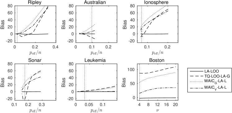
Figure 1: Bias when the ground truth is exact LOO with Laplace (LA in Table4) and varying flexibility of the model, or degrees of freedom in the Student’s $t$ model for the Boston data. Model flexibility was varied by rescaling the length scale(s) in the GP model. Model flexibility is measured by the relative effective number of parameters $p_{\rm eff}/n$. The flexibility of the MAP model is shown with a vertical dashed line. For the Student’s $t$ model the vertical dashed line is at $\nu=4$.

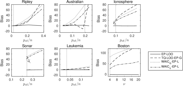
Figure 2: Bias when the ground truth is exact LOO with EP (EP in Table4) and varying flexibility of the model, or degrees of freedom in the Student’s $t$ model for the Boston data. Model flexibility was varied by rescaling the length scale(s) in the GP model. Model flexibility is measured by the relative effective number of parameters $p_{\rm eff}/n$. The flexibility of the MAP model is shown with a vertical dashed line. For the Student’s $t$ the vertical dashed line is at $\nu=4$.

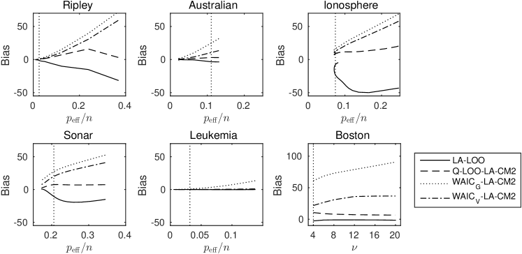
Figure 3: Bias when the ground truth is exact LOO with Laplace-CM2 (LA-CM2 in Table4) and varying flexibility of the model, or degrees of freedom in the Student’s $t$ model for the Boston data. Model flexibility was varied by rescaling the length scale(s) in the GP model. Model flexibility is measured by the relative effective number of parameters $p_{\rm eff}/n$. The flexibility of the MAP model is shown with a vertical dashed line. For the Student’s $t$ the vertical dashed line is at $\nu=4$.

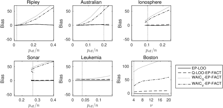
Figure 4: Bias when the ground truth is exact LOO with EP-FACT (EP-FACT in Table4) and varying flexibility of the model, or degrees of freedom in the Student’s $t$ model for the Boston data. Model flexibility was varied by rescaling the length scale(s) in the GP model. Model flexibility is measured by the relative effective number of parameters $p_{\rm eff}/n$. The flexibility of the MAP model is shown with a vertical dashed line. For the Student’s $t$ the vertical dashed line is at $\nu=4$.

4.4 Approximate LOO comparison to exact LOO – hierarchical model

Next we examine the accuracy of hierarchical LOO approximation of $p(y_{i}|x_{i},D_{-i})$ (see Section 3.2), where the conditional LOO densities $p(y_{i}|x_{i},D_{-i},\theta,\phi)$ are approximated with LA-LOO or EP-LOO, which we found performed best for conditional densities (see previous section).

Table 9 shows the results when the ground truth is exact LOO with CCD used to integrate over the parameter posterior and the Laplace method is used to integrate over the latent values (LA+CCD in Table 4). The Laplace approximation combined with type II MAP parameter estimates or CCD integration but no importance weighting has an error size related to the number of hyperparameters $(\theta,\phi)$. The unweighted CCD or MAP gives a small error only if the number of parameters $(\theta,\phi)$ is small. Importance weighting of CCD works well for all data sets except Australian and Boston. These data sets have more parameters (17) than the others (4-8), making the inference more difficult. The minimum relative effective sample sizes (Ripley=60%, Australian=16%, Ionosphere=59%, Sonar=70%, Leukemia=36%, Boston=0.3%) correctly indicate that importance weighting for Australian and Boston data sets is unreliable.

Table 10 shows the corresponding results when the ground truth is exact LOO with CCD used to integrate over the parameter posterior and expectation propagation used to integrate over the latent values (EP+CCD in Table 4). EP with the unweighted CCD or MAP gives a small error only if the number of parameters $(\theta,\phi)$ is small. Importance weighting of CCD works well for all data sets except Australian and Boston. Again the minimum relative effective sample sizes (Ripley=60%, Australian=12%, Ionosphere=36%, Sonar=65%, Leukemia=35%, Boston=9%) correctly indicate that importance weighting for Australian and Boston is unreliable.

As CCD integration provided good results for exact LOO (Table 4), the larger errors of CCD+IS for the Australian and Boston data is not due to CCD itself failing, but importance weighting failing. As an additional check we sampled the hyperparameters with MCMC (6000 samples with slice sampling) and computed Pareto smoothed importance sampling estimates (MCMC+PSIS) shown also in Tables 9 and 10. Due to larger number of samples, the errors are slightly reduced, but still for the Australian and Boston data sets the errors are larger. The PSIS diagnostics (maximum of Pareto shape parameters $\hat{k}$ for Laplace: Ripley=$0.4$, Australian=$1.2$, Ionosphere=$0.4$, Sonar=$0.4$, Leukemia=$0.2$, Boston=$1.3$; for EP: Ripley=$0.3$, Australian=$1.6$, Ionosphere=$0.3$, Sonar=$0.3$, Leukemia=$0.2$, Boston=$0.7$) correctly indicate the problematic cases ($\hat{k}>0.7$).

If the minimum relative effective sample size or PSIS diagnostics warn about potential problems, depending on the application it may be necessary to run, for example, $k$-fold cross-validation.

Method	Ripley	Australian	Ionosphere	Sonar	Leukemia	Boston
LA-LOO+MCMC+PSIS	0.08 (0.15)	-1.1 (2.3)	0.2 (0.1)	0.1 (0.2)	-0.04 (0.19)	-6.1 (2.4)
LA-LOO+CCD+IS	0.18 (0.10)	3.4 (0.4)	-0.1 (0.1)	-0.13 (0.06)	0.56 (0.05)	-5.2 (5.0)
LA-LOO+CCD	0.8 (0.2)	7.2 (0.9)	0.6 (0.2)	0.5 (0.2)	4.8 (0.2)	17 (3)
LA-LOO+MAP	1.0 (0.2)	9.2 (1.8)	1.3 (0.2)	1.3 (0.3)	4.9 (0.6)	15 (3)

Table 9: Bias and standard deviation when the ground truth is exact LOO with Laplace and CCD (LA+CCD in Table 4). Bolded values have significantly smaller absolute error than the values from the other methods for the same data set.

Method	Ripley	Australian	Ionosphere	Sonar	Leukemia	Boston
EP-LOO+MCMC+PSIS	0.38 (0.17)	-2.4 (3.4)	0.8 (0.5)	-0.23 (0.22)	-0.16 (0.23)	-0.9 (1.0)
EP-LOO+CCD+IS	0.42 (0.14)	7.3 (1.4)	0.8 (0.6)	-0.24 (0.14)	0.49 (0.04)	2.2 (1.0)
EP-LOO+CCD	1.3 (0.4)	15 (2)	2.8 (1.3)	0.6 (0.3)	4.8 (0.2)	20 (2)
EP-LOO+MAP	1.4 (0.3)	17 (2)	2.8 (0.7)	0.9 (0.3)	4.9 (0.6)	17 (2)

Table 10: Bias and standard deviation when the ground truth is exact LOO with EP and CCD (EP+CCD in Table 4). Bolded values have significantly smaller absolute error than the values from the other methods for the same data set.

5 Discussion

We have shown that LA-LOO and EP-LOO provide fast and accurate conditional LOO results when the predictions at new points are made using the Gaussian latent value distribution. If the predictions at new points are made using non-Gaussian distributions obtained from the global correction, then quadrature LOO gives useful results, but it would be faster and more accurate to just use EP without the global correction. Both Laplace-LOO and EP-LOO can be combined with importance sampling or importance weighted CCD to get fast and accurate full Bayesian leave-one-out cross-validation results.

If other methods than LA-LOO or EP-LOO are used, we propose the following rule of thumb for diagnostics: The methods other than LA-LOO and EP-LOO start to fail when the relative effective number of parameters ($p_{\rm eff}/n$) is larger than 2%–5%.

Here we have considered fully factorizing likelihoods, but the methods can be extended for use with likelihoods with grouped factorization, such as in multi-class classification, multi-output regression, and some hierarchical models with lowest level grouping. We assume that the accuracy using Laplace-LOO and EP-LOO would also be good in these cases.

In this paper, we have concentrated on how well exact LOO can be estimated with fast approximations. LOO is useful for estimating the predictive performance of of a model or in model comparison, but it should not be used to select a single model among a large number of models due to a selection induced bias as demonstrated by Piironen and Vehtari (2016).

Appendix A Linear response Laplace leave-one-out

Using linear response theory, used by Opper and Winther (2000) to prove LOO consistency of EP, we here derive approximative Laplace leave-one-out equations.

The idea is to express the posterior mode solution for the LOO problem in terms of the solution for the full problem. The computationally cheap solution can be obtained by making the assumption that the difference between these two solutions is small such that their difference may be treated as a second order Taylor expansion. We will give two different derivations of the result stated in Section 3.5; One is based on a second order expansion of the log likelihood and the second on a classical linear response argument.

In the expansion approach we make the approximation that when example $i$ is removed we can treat the change in the mode for the remaining variables to second order. The log prior is already quadratic so it is only the non-linearity in the log likelihood terms $j\neq i$ that we expand to second order:

$$\log p(y_{j}|f_{j},\phi)\approx\log p(y_{j}|\hat{f}_{j},\phi)+(f_{j}-\hat{f}_{j})\nabla_{j}\log p(y_{j}|f_{j},\phi)|_{f_{j}=\hat{f_{j}}}-\frac{(f_{j}-\hat{f}_{j})^{2}}{2\tilde{\Sigma}_{j}}\ ,$$ (65)

where $\tilde{\Sigma}_{j}$ is defined in Equation (14). We collect the first and second order contributions of the expansion to give the Gaussian type leave $i$ out factors for the likelihood terms $j\neq i$. We recognize that these approximate factors coincide with those introduced in the full Laplace approximation in Equation (8). We can now write the approximate leave one out posterior as

$$q(f|D_{-i},\theta,\phi)\propto\prod_{j\neq i}\tilde{t}_{j}(f_{j})p(f|X,\theta)$$ (66)

and the marginal as

$$p(f_{i}|D_{-i},\theta,\phi)\approx q_{-i}(f_{i}) \propto\frac{1}{\tilde{t}_{i}(f_{i})}\int\prod_{j}\tilde{t}_{j}(f_{j})p(f|X,\theta)df_{-i}$$

$$\propto\frac{1}{\tilde{t}_{i}(f_{i})}\int{\operatorname{N}}(f|\hat{f},\hat{\Sigma})df_{-i}=\frac{{\operatorname{N}}(f_{i}|\hat{f}_{i},\hat{\Sigma}_{ii})}{\tilde{t}_{i}(f_{i})}\ .$$ (67)

This result shows that in a self-consistent second order approximation, where we take into account both the explicit removal of likelihood term $i$ and the implicit effect on the remaining variables, the leave one out posterior is obtained simply by dividing by the Gaussian factor for $i$. Finally we complete the square and obtain the result in Equation (38).

Next we show how the same result can be obtained by a linear response argument. The equation for the mode is

$$K^{-1}\hat{{f}}=\hat{{g}}\ ,$$ (68)

where $\hat{{g}}=\nabla\log p({y}|\hat{f},\phi)$ is the vector of derivatives of the terms in the log likelihood (depending non-linearly on $\hat{f}$). Because this defines an equation for the mode, we only need to make a variation to first order in this case to recover the result we obtained above. When we remove likelihood term $i$ the change in the mode can be written as

$$K^{-1}\delta\hat{{f}}=\delta\hat{{g}}$$ (69)

with the change in $\hat{g}$ to first order

$$\delta\hat{{g}}\approx-\tilde{\Sigma}^{-1}\delta\hat{f}+e_{i}\tilde{\Sigma}^{-1}_{i}\delta\hat{f}_{i}-e_{i}\hat{g}_{i},$$ (70)

where we have used $\frac{\partial\hat{g}_{i}}{\partial\hat{f}_{i}}=-\hat{h}_{i}=-\tilde{\Sigma}^{-1}_{i}$ and $e_{i}$ is a unit vector in the $i$th direction. The first two terms on the right hand side are the indirect change of the equation due to the removal of term $i$ and the last is the direct contribution. We can now solve the linearized equation with respect to $\delta\hat{f}$ using the definition of the Laplace covariance $\Sigma=(K^{-1}+\tilde{\Sigma}^{-1})^{-1}$

$$\delta\hat{f}=\Sigma e_{i}(\tilde{\Sigma}^{-1}_{i}\delta\hat{f}_{i}-\hat{g}_{i}).$$ (71)

Specializing to $\delta\hat{f}_{i}$ we get

$$\delta\hat{f}_{i}=\Sigma_{ii}(\tilde{\Sigma}^{-1}_{i}\delta\hat{f}_{i}-\hat{g}_{i})$$ (72)

which can be solved with respect to $\delta\hat{f}_{i}$ to give $\delta\hat{f}_{i}=-v_{-i}\hat{g}_{i}$. This is in agreement with the change in the mode equation (38) we found above. The variance term can be derived with a related linear response argument (Opper and Winther, 2000).

Appendix B Computational complexities

We summarize here the computational complexities of different methods in the paper. We first summarize the computational complexities of the Laplace method, expectation propagation, and marginal approximations used to obtain the full data posterior and its marginals. Then we summarize the additional computational complexities of the LOO methods. The related practical speed comparison results are shown in Appendix C.

The computational complexity for both the Laplace method and EP for GLVMs is dominated by matrix computations related to the covariance or precision matrix. We denote this basic cost as $c_{\rm{basic}}$. For GLVMs with a full rank dense covariance matrix (such as Gaussian processes used in Section 4), $c_{\rm{basic}}$ scales with $n^{3}$. For reduced rank approximations in Gaussian processes such as FITC (Quiñonero-Candela and Rasmussen, 2005), $c_{\rm{basic}}$ scales with $m^{2}n$, where $m\ll n$ is the reduced rank (affecting the flexibility of GP). For sparse precision (in Gaussian Markov random field models (see, e.g., Rue et al., 2009)) or covariance matrices (in compact support covariance function GPs (see, e.g., Vanhatalo and Vehtari, 2008)), $c_{\rm{basic}}$ scales with $n_{\rm{nonzeros}}^{2}$, where $n<n_{\rm{nonzeros}}<n^{2}/2$ is the number of non-zeros in the precision, covariance, or Cholesky matrix (see more detailed analysis of sparse GLVMs in Cseke and Heskes, 2011).

For fixed $\phi$ and $\theta$, the computation of the conditional posterior and marginal likelihoods scales for the Laplace method with $n^{\rm{Newton}}_{\rm{steps}}\times c_{\rm{basic}}$ and for EP with $n^{\rm{EP}}_{\rm{steps}}\times(c_{\rm{basic}}+n\times n_{\rm{quad}})$, where $n_{\rm{quad}}$ is the number of potential quadrature evaluations to compute moments (for a probit classification model the moments can be computed in closed form).

After the last step of the Newton or EP algorithm, the additional computational complexities for different LOO methods are shown in Table 11. EP-LOO has zero additional complexity as the LOO log predictive density is computed as part of the algorithm. LA-LOO and methods using Gaussian marginals require $n$ quadrature integrals to obtain log predictive densities and thus have negligible additional complexity. EP-FACT and LA-CM2 based methods have significantly larger additional complexity. The additional complexity of EP-FACT based methods scale with $n^{2}\times n_{\rm{quad,1}}\times n_{\rm{quad,2}}$, where $n_{\rm{quad,1}}$ and $n_{\rm{quad,2}}$ refer to two different quadratures in the method. The additional complexity of LA-CM based methods scale with $n\times c_{\rm{basic}}\times n_{\rm{quad}}>n^{3}\times n_{\rm{quad}}$, which can be more than the complexity for the conditional posterior.

Method	Additional computational complexity
EP-LOO	$0$
LA-LOO	$n\times n_{\rm{quad}}$
(T)Q-LOO-LA/EP-G	$n\times n_{\rm{quad}}$
$\mathrm{WAIC}_{G/V}$-LA/EP-G/L	$n\times n_{\rm{quad}}$
(T)Q-LOO-EP-FACT	$n^{2}\times n_{\rm{quad,1}}\times n_{\rm{quad,2}}$
$\mathrm{WAIC}_{G/V}$-EP-FACT	$n^{2}\times n_{\rm{quad,1}}\times n_{\rm{quad,2}}$
(T)Q-LOO-LA-CM2	$n\times c_{\rm{basic}}\times n_{\rm{quad}}$
$\mathrm{WAIC}_{G/V}$-LA-CM2	$n\times c_{\rm{basic}}\times n_{\rm{quad}}$
Exact brute force LOO EP	$n\times(n^{\rm{EP}}_{\rm{steps}}\times(c_{\rm{basic}}+n\times n_{\rm{quad}}))$
Exact brute force LOO Laplace	$n\times(n^{\rm{Newton}}_{\rm{steps}}\times c_{\rm{basic}}+n_{\rm{quad}})$

Table 11: Additional computational complexity of LOO methods for fixed $\theta$ and $\phi$ after obtaining the full posterior approximation with the Laplace method or EP.

The computational complexity for the Type II MAP solution is the computational complexity of forming the conditional posterior given $\theta$ and $\phi$ times the number of marginal posterior evaluations in optimisation. The additional computation to obtain LOO after Type II MAP is the computation of LOO with fixed $\theta$ and $\phi$.

The computational complexity for integration over the marginal posterior of $\theta$ and $\phi$ is the computational complexity of forming the conditional posterior given $\theta$ and $\phi$ times the number of marginal posterior evaluations in the (deterministic or stochastic) algorithm forming the posterior approximation. The additional computation for LOO requires the computation of LOO with fixed $\theta$ and $\phi$ for each point in the final marginal posterior approximation and computation of importance weights which has a negligible additional cost.

Appendix C Practical speed comparison

To further give some idea of the practical speed differences between the different algorithm implementations we show examples of computation times for computing the marginal likelihood and LOO given fixed $\theta$ and $\phi$. The speed comparisons were run with a laptop (Intel Core i5-4300U CPU @ 1.90GHz x 4 + 8GB memory). As one of the reviewers was interested in comparison to global Gaussian variational method, we have included it in this speed comparison, verifying the previous results that it is much slower than EP (Nickisch and Rasmussen, 2008). As GPstuff does not have the global Gaussian variational approximation, we use the KL method in GPML toolbox (Rasmussen and Nickisch, 2010) to compute that. To take into account potential general speed differences between GPstuff and GPML we also timed GPML Laplace and EP methods. Computations were timed several times so that caching of the previous computations were not used.

Table 12 shows the time to compute the latent posterior and marginal likelihood with fixed hyperparameters. In optimization (or gradient based MCMC), the computation of gradients would have additional computational cost. When hyperparameters are integrated out, the approximative computation time is these multiplied by the number of unique parameter values evaluated when obtaining the marginal posterior samples (there are additional overheads and potential speed-ups). For probit, where the moments required in EP can be computed analytically, GPstuff-EP is about 1.5–5 times slower than GPstuff-LA. For log-logistic with censoring GPstuff-EP is about 18 times slower due to slow quadrature based moment computations (which could be made faster). For the Student’s $t$ model GPstuff-LA and GPstuff-EP have similar performance, as the robust Laplace-EM method by Vanhatalo et al. (2009) is slower than basic Laplace approximation. GPstuff-LA and GPML-LA have quite similar speed, GPstuff being slightly faster. GPstuff-EP is 10-25 times faster than GPML-EP, which is probably due to using parallel updates and better vectorization allowed by parallel updates. GPstuff has robust-EP implementation which also works for non-log-concave likelihoods such as Student’s $t$. Although KL has the same $O(n^{3})$ computational scaling as EP, its computational overhead makes GPML-KL 70-500 times slower than GPML-EP.

				GPstuff		GPML
Data set	n	d	lik	LA	EP1	LA	EP2	KL
Ripley	250	2	probit	0.02	0.04	0.06	0.71	155
Australian	690	14	probit	0.13	0.40	0.26	10	704
Ionosphere	351	33	probit	0.05	0.13	0.08	1.7	516
Sonar	208	60	probit	0.03	0.04	0.06	0.47	233
Leukemia	1043	4	log-logistic w. cens.	0.18	3.5	NA3	NA3	NA3
Boston	506	13	Student’s $t$	1.14	1.1	NA5	NA6	397

Table 12: Time (in seconds) to compute the posterior and marginal likelihood with fixed hyperparameters. ¹GPstuff uses parallel EP (van Gerven et al., 2009) except for Student’s $t$ parallel robust-EP (Jylänki et al., 2011) is used. ²GPML uses random order sequential EP (Rasmussen and Williams, 2006). ³GPML does not have log-logistic model with censoring. ⁴For Student’s $t$ Laplace-EM method (Vanhatalo et al., 2009) was used. ⁵The GPML’s Laplace inference algorithm did run without errors, but the results were really bad (difference in LOO-LPD $1.4e4$). ⁶GPML does not support EP for non-log-concave likelihoods. ⁷For Student’s $t$ the performance of global Gaussian variational (KL) method was much worse than the performance of Laplace-EM and EP (difference in LOO-LPD $147$)

Table 13 shows time to compute the LOO for fixed parameters after the full posterior has been computed (see Table 12). When hyperparameters are integrated out, the approximative computation time is these multiplied by the number of parameter samples approximating the marginal posterior. There is no added computational cost of going from EP to EP-LOO and the time is spent retrieving the stored result. The computational cost of LA-LOO is computing cavity distributions and one quadrature. Here Q-LOO computations also include the time to compute the marginal corrections (LA-CM2 and EP-FACT), which make them much slower.

			Q-LOO-	Q-LOO-	Exact LOO	Exact LOO
Data set	LA-LOO	EP-LOO	LA-CM2	EP-FACT	Laplace	EP
Ripley	0.01	0.005	30	3.7	6.3	13
Australian	0.11	0.005	672	15	90	323
Ionosphere	0.03	0.005	91	6.1	19	47
Sonar	0.02	0.005	19	3.0	7.2	12
Leukemia	0.89	0.005	2547	11876	198	3762
Boston	0.47	0.005	237	7.5	583	587

Table 13: Time (in seconds) to compute LOO for fixed parameters after the full posterior has been computed. Here Q-LOO computations also include the time to compute the marginal corrections (LA-CM2 and EP-FACT).

References

- An (1998) Mark Yuying An. Logconcavity versus logconvexity: a complete characterization. Journal of Economic Theory, 80(2):350–369, 1998.
- Bernardo and Smith (1994) José M. Bernardo and Adrian F. M. Smith. Bayesian Theory. John Wiley & Sons, 1994.
- Challis and Barber (2013) Edward Challis and David Barber. Gaussian Kullback-Leibler approximate inference. Journal of Machine Learning Research, 14:2239–2286, 2013.
- Cseke and Heskes (2011) Botond Cseke and Tom Heskes. Approximate marginals in latent Gaussian models. Journal of Machine Learning Research, 12:417–454, 2 2011. ISSN 1532-4435.
- Epifani et al. (2008) Ilenia Epifani, Steven N MacEachern, and Mario Peruggia. Case-deletion importance sampling estimators: Central limit theorems and related results. Electronic Journal of Statistics, 2:774–806, 2008.
- Geisser and Eddy (1979) Seymour Geisser and William F. Eddy. A predictive approach to model selection. Journal of the American Statistical Association, 74(365):153–160, March 1979.
- Gelfand (1996) Alan E. Gelfand. Model determination using sampling-based methods. In W. R. Gilks, S. Richardson, and D. J. Spiegelhalter, editors, Markov Chain Monte Carlo in Practice, pages 145–162. Chapman & Hall, 1996.
- Gelfand et al. (1992) Alan E. Gelfand, D. K. Dey, and H. Chang. Model determination using predictive distributions with implementation via sampling-based methods (with discussion). In J. M. Bernardo, J. O. Berger, A. P. Dawid, and A. F. M. Smith, editors, Bayesian Statistics 4, pages 147–167. Oxford University Press, 1992.
- Gelman et al. (2013) Andrew Gelman, John B. Carlin, Hal S. Stern, David B. Dunson, Aki Vehtari, and Donald B. Rubin. Bayesian Data Analysis. Chapman & Hall/CRC, third edition, 2013.
- Gelman et al. (2014) Andrew Gelman, Jessica Hwang, and Aki Vehtari. Understanding predictive information criteria for Bayesian models. Statistics and Computing, 24(6):997–1016, 2014.
- Gneiting and Raftery (2007) Tilmann Gneiting and Adrian E. Raftery. Strictly proper scoring rules, prediction, and estimation. Journal of American Statistical Association, 102:359–379, 2007.
- Gneiting et al. (2007) Tilmann Gneiting, Fadoua Balabdaoui, and Adrian E Raftery. Probabilistic forecasts, calibration and sharpness. Journal of the Royal Statistical Society: Series B (Statistical Methodology), 69(2):243–268, 2007.
- Held et al. (2010) Leonhard Held, Birgit Schrödle, and Håvard Rue. Posterior and cross-validatory predictive checks: A comparison of MCMC and INLA. In Thomas Kneib and Gerhard Tutz, editors, Statistical Modelling and Regression Structures, pages 91–110. Springer, 2010.
- Hernáandez-Lobato et al. (2010) Daniel Hernáandez-Lobato, José M. Hernández-Lobato, and Alberto Suárez. Expectation propagation for microarray data classification. Pattern Recognition Letters, 31(12):1618–1626, 2010.
- Hernández-Lobato et al. (2008) José M. Hernández-Lobato, Tjeerd Dijkstra, and Tom Heskes. Regulator discovery from gene expression time series of malaria parasites: a hierarchical approach. In J.C. Platt, D. Koller, Y. Singer, and S. Roweis, editors, Advances in Neural Information Processing Systems 20, pages 649–656, 2008.
- Ionides (2008) Edward L. Ionides. Truncated importance sampling. Journal of Computational and Graphical Statistics, 17(2):295–311, 2008.
- Jylänki et al. (2011) Pasi Jylänki, Jarno Vanhatalo, and Aki Vehtari. Robust Gaussian process regression with a Student- likelihood. Journal of Machine Learning Research, 12:3227–3257, 2011.
- Kingma and Welling (2014) Diederik P Kingma and Max Welling. Auto-encoding variational Bayes. The International Conference on Learning Representations (ICLR), 2014.
- Kong et al. (1994) Augustine Kong, Jun S. Liu, and Wing Hung Wong. Sequential imputations and Bayesian missing data problems. Journal of the American Statistical Association, 89(425):278–288, 1994.
- Koopman et al. (2009) Siem Jan Koopman, Neil Shephard, and Drew Creal. Testing the assumptions behind importance sampling. Journal of Econometrics, 149(1):2–11, 2009.
- Li et al. (2014) Longhai Li, Shi Qiu, Bei Zhang, and Cindy X. Feng. Approximating cross-validatory predictive evaluation in Bayesian latent variables models with integrated IS and WAIC. arXiv preprint arXiv:1404.2918, 2014.
- Lindgren and Rue (2015) Finn Lindgren and Håvard Rue. Bayesian spatial modelling with R-INLA. Journal of Statistical Software, 63(19), 2015.
- Marshall and Spiegelhalter (2003) E. C. Marshall and D. J. Spiegelhalter. Approximate cross-validatory predictive checks in disease mapping models. Statistics in Medicine, 22(10):1649–1660, 2003.
- Martins et al. (2013) Thiago G Martins, Daniel Simpson, Finn Lindgren, and Håvard Rue. Bayesian computing with INLA: new features. Computational Statistics & Data Analysis, 67:68–83, 2013.
- Minka (2001) Thomas Minka. A Family of Algorithms for Approximate Bayesian Inference. PhD thesis, Massachusetts Institute of Technology, 2001.
- Murray and Adams (2010) Iain Murray and Ryan Prescott Adams. Slice sampling covariance hyperparameters of latent Gaussian models. In J. Lafferty, C. K. I. Williams, R. Zemel, J. Shawe-Taylor, and A. Culotta, editors, Advances in Neural Information Processing Systems 23, pages 1732–1740, 2010.
- Murray et al. (2010) Iain Murray, Ryan Prescott Adams, and David J.C. MacKay. Elliptical slice sampling. JMLR Workshop and Conference Proceedings: Proceedings of the Thirteenth International Conference on Artificial Intelligence and Statistics, 9:541–548, 2010.
- Nickisch and Rasmussen (2008) Hannes Nickisch and Carl Edward Rasmussen. Approximations for binary Gaussian process classification. Journal of Machine Learning Research, 9:2035–2078, October 2008.
- Opper and Winther (2000) Manfred Opper and Ole Winther. Gaussian processes for classification: Mean-field algorithms. Neural Computation, 12(11):2655–2684, 2000.
- Peruggia (1997) Mario Peruggia. On the variability of case-deletion importance sampling weights in the Bayesian linear model. Journal of the American Statistical Association, 92(437):199–207, 1997.
- Piironen and Vehtari (2016) Juho Piironen and Aki Vehtari. Comparison of Bayesian predictive methods for model selection. Statistics and Computing, 2016. Online first: DOI:10.1007/s11222-016-9649-y.
- Quiñonero-Candela and Rasmussen (2005) Joaquin Quiñonero-Candela and Carl Edward Rasmussen. A unifying view of sparse approximate Gaussian process regression. Journal of Machine Learning Research, 6(3):1939–1959, 2005.
- Ranganath et al. (2014) Rajesh Ranganath, Sean Gerrish, and David M Blei. Black box variational inference. JMLR Workshop and Conference Proceedings: Proceedings of the Seventeenth International Conference on Artificial Intelligence and Statistics, 33:814–822, 2014.
- Rasmussen and Nickisch (2010) Carl Edward Rasmussen and Hannes Nickisch. Gaussian processes for machine learning (GPML) toolbox. The Journal of Machine Learning Research, 11:3011–3015, 2010.
- Rasmussen and Williams (2006) Carl Edward Rasmussen and Christopher K. I. Williams. Gaussian Processes for Machine Learning. The MIT Press, 2006.
- Rezende et al. (2014) Danilo Jimenez Rezende, Shakir Mohamed, and Daan Wierstra. Stochastic backpropagation and approximate inference in deep generative models. JMLR Workshop and Conference Proceedings: Proceedings of The 31st International Conference on Machine Learning, 32:1278–1286, 2014.
- Riihimäki and Vehtari (2014) Jaakko Riihimäki and Aki Vehtari. Laplace approximation for logistic Gaussian process density estimation and regression. Bayesian analysis, 9(2):425–448, 2014.
- Riihimäki et al. (2013) Jaakko Riihimäki, Pasi Jylänki, and Aki Vehtari. Nested expectation propagation for Gaussian process classification with a multinomial probit likelihood. Journal of Machine Learning Research, 14:75–109, 2013.
- Rue et al. (2009) Håvard Rue, Sara Martino, and Nicolas Chopin. Approximate Bayesian inference for latent Gaussian models by using integrated nested Laplace approximations. Journal of the Royal statistical Society B, 71(2):1–35, 2009.
- Seeger (2008) Matthias Seeger. Bayesian inference and optimal design for the sparse linear model. Journal of Machine Learning Research, 9:759–813, 2008.