SEARCH VIA QUANTUM WALKS WITH INTERMEDIATE MEASUREMENTS

Abstract

A modification of Tulsi’s quantum search algorithm with intermediate measurements of the control is presented. In order to analyze the effect of measurements in quantum searches, a different choice of the angular parameter is used. The study is performed for several values of time lapses between measurements, finding close relationships between probabilities and correlations (Mutual Information and Cumulative Correlation Measure). The order of this modified algorithm is estimated, showing that for some time lapses the performance is improved, and became of order $O(N)$ (classical brute force search) when the measurement is taken in every step. The results indicate a possible way to analyze improvements to other quantum algorithms using one, or more, control qubits.

I Introduction

Although there is no consensus on what are the quantum properties that cause the advantage of a quantum algorithm over classical counterparts, this advantage has been associated mainly with quantum correlation (concepts as entanglement, quantum discord, non-locality, contextuality and others)Nest_2013 . While it is believed that some quantum correlation is necessary in quantum search, it is not exactly clear how correlation is related with good resultsCui_2010 . Correlation is modified by measurements and interaction with the environment, generally modeled as noiseNielsen_2000 , whose influence on quantum search algorithms has been extensively studied in last yearsRomanelli_2005 ; Salas_2008 ; Abal_2009 ; Srikanth_2010 ; Gawron_2012 . Furthermore, some research has been done to analyze the effect of projective partial measurements of the systemTulsi_2006 ; Maloyer_2007 .

It has been generally assumed that decoherence degrades the efficiency of a quantum algorithm. Nevertheless, in recent years some studies have shown that low levels of noise can improve certain algorithmsKendon_2007 ; Venegas_Andraca_2012 . Would this be the case of projective partial measurements in quantum searches? In this article we show that the effect of intermediate partial measurements during the state evolution can improve the performance of some search algorithms, i.e. controlled quantum walk search algorithms. In addition, we show there is a close relationships between the search results and correlations.

The proposed quantum search is an intermediate case between two known methods: unitary algorithms that starts with separable statesPortugal_2013 , where the correlation increases during the evolution; and Measurement Based Quantum Computation (MBQC)Raussendorf_2003 , where the initial states are of high correlation (cluster states), and measurements are taken to achieve the desired results.

Tulsi’s algorithmTulsi_2008 is an special case of the abstract search algorithm based on a discrete quantum walk, that uses a control qubit in addition to the usual coin. This quantum walk depends on an angular parameter $\delta$, where the optimum value ensures an order of $O(\sqrt{N\log N})$, considering a $\sqrt{N}\times\sqrt{N}$ search grid.

In this article a modified instance of Tulsi’s algorithm, in a Hilbert space $\mathcal{H}=(\mathbb{C}^{2})^{\otimes m}$, is used with the main purpose of analyze the influence of partial intermediate measurement in quantum algorithms. With this aim, and considering that Tulsi’s algorithm is optimal, a different choice of the angular parameter $\delta$ is made. Based on numerical evidence, it has been found that a unitary algorithm can be improved by performing partial projective measurements with a convenient choice of time lapses between unitary evolutions. Relationship among the time between intermediate measurements, the correlation, and the order of the algorithm is discussed.

The paper is organized as follows. In order to introduce the notation and operators used, Tulsi’s algorithm is briefly explained in Section 2. Modified Tulsi’s algorithm with intermediate partial measurements is presented in Section 3. Section 4 deals with the relation between probabilities and correlations. In Section 5, the order of the presented algorithm is estimated depending on time lapse between measurements. Finally, some conclusions and proposals for future works are commented in Section 6.

II Unitary Tulsi algorithm

Tulsi’s quantum walk based algorithm searches an unique item out of $N$ items arranged on a two-dimensional ($\sqrt{N}\times\sqrt{N}$) grid. This position space is represented by an n-qubit quantum state ($N=2^{n}$), and it is initialized with a state formed by an uniform superposition of the canonical basis, similar to GroverGrover_1996 and AKRAKR_2005 quantum algorithms. In addition to the position, the state has a two qubits coin state and a control qubit (initialized as indicated in (6)).

The Tulsi’s algorithm uses two operators: the oracle and the the conditional walk. The conditioned reflection operator, called oracle, is given by,

$$O=I-2\,|\delta_{ctr},u_{c},t\rangle\langle\delta_{ctr},u_{c},t|$$ (1)

where

• the control qubit $|\delta_{ctr}\rangle=-\sin\delta|0\rangle+\cos\delta|1\rangle$, depends on the $\delta$ parameter,

• the coin state $|u_{c}\rangle$ is a balanced superposition of two qubits in the coin basis $\{|i_{c}\rangle\}=\{\leftarrow,\rightarrow,\downarrow,\uparrow\}$

  $$|u_{c}\rangle=\frac{1}{2}\sum_{i_{c}=0}^{3}|i_{c}\rangle,$$ (2)

• and the target state $|t\rangle$ is any unknown state of the position subspace.

The conditional walk operator performs a walk depending on the value of the control qubit, as showed in the following equation

$$W=|1\rangle\langle 1|\otimes(S\cdot C)-|0\rangle\langle 0|\otimes I_{c,p}$$ (3)

where

• $S$ is the shift operator

  $$S=\sum_{x,y}|\leftarrow,x+1,y\rangle\langle\rightarrow,x,y|+|\downarrow,x,y+1\rangle\langle\uparrow,x,y|+$$

  $$|\rightarrow,x-1,y\rangle\langle\leftarrow,x,y|+|\uparrow,x,y-1\rangle\langle\downarrow,x,y|$$

  being the state $|x,y\rangle$ related to the $x,y$ position on the grid,

• $C$ operates only in the coin subspaceAKR_2005

  $$C_{0}=-I_{c}+2|u_{c}\rangle\langle u_{c}|$$ (5)

  where $C=C_{0}\otimes I_{p}$.

As proved in Tulsi_2008 , considering an initial state $|\psi_{0}\rangle$

$$|\psi_{0}\rangle=|1,u_{c},u_{p}\rangle=|1\rangle\otimes|u_{c}\rangle\otimes|u_{p}\rangle=|1\rangle\otimes|u_{c}\rangle\otimes\frac{1}{\sqrt{N}}\sum_{i_{p}=0}^{N-1}|i_{p}\rangle,$$ (6)

and applying $T_{\delta}=[\frac{\pi}{4}\sqrt{N(\log{N}+\tan{\delta}^{2}/4)}]$ times (steps) the operator $U=W.O$ (Fig. 1), the evolving state approaches the target state. The main result is that the overlap between the final state and the target state depends on $\delta$ and $N$. By choosing parameter $\delta$ as $\cos(\delta)=1/\log{N}$, the target probability becomes independent of $N$, and the algorithm has an order $O(\sqrt{N\log{N}})$.

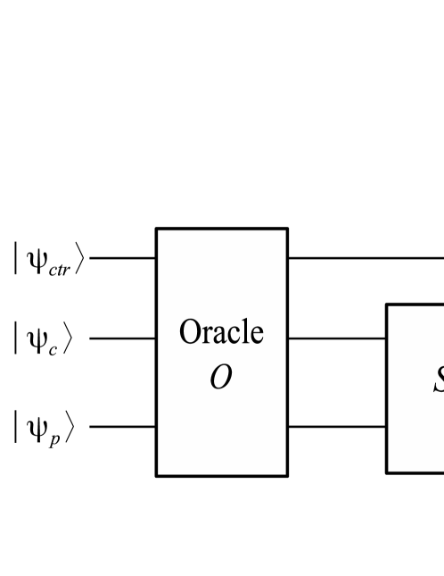
Figure 1: Tulsi algorithm

For a $2^{9}\times 2^{9}$ grid ($N=2^{18}$), and three angular parameters choices ($\delta=0$, $\delta=\pi/4$ and the Tulsi’s parameter $\delta=\arccos\left(1/{\sqrt{\log{N}}}\,\right)$), the resulting probabilities are shown in Figure (2).

Figure 2: Unitary evolution of Tulsi algorithm with $N=2^{18}$ and: $\delta=0$ (AKR with dots), $\delta=\pi/4$ (dash line) and $\delta=\arccos({\sqrt{1/\log{N}}})$ (solid line).

III Intermediate measurements algorithm

Unlike Tulsi’s unitary algorithm, our proposal (Figure (3)) consists in taking projectives measurements of the control qubit, at time-lapses $l$, between unitary evolutions. The aim is to understand how intermediate partial measurements affect the target probability, and its relationship with correlation.

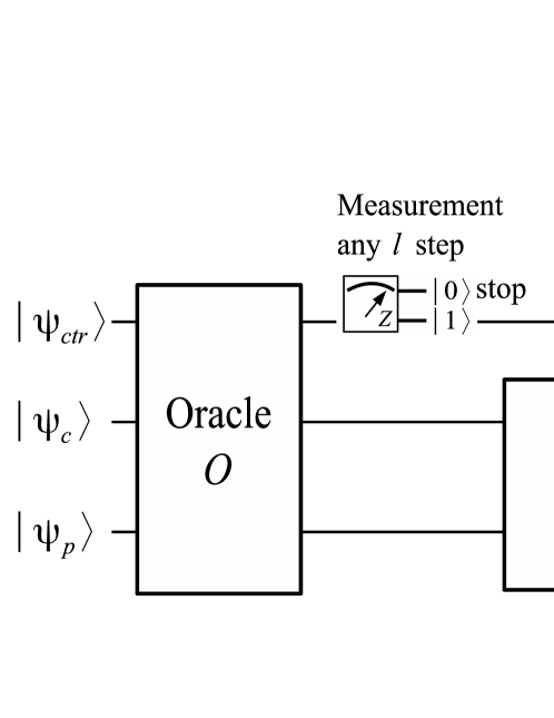
Figure 3: Intermediate measurements algorithm: $IMA$

After any measurement is performed, the obtained information allows to stop the algorithm if the result is $0$, since this control value is exclusively related to the target state position. This can be seen as the result of applying the sequence of operators (1) and (3) to a basis state $|i_{ctr},i_{c},i_{p}\rangle$. In the case where $|i_{p}\rangle$ is any position basis state different from the target position we have

$$|1,i_{c},i_{p}\rangle\xrightarrow{O}|1,i_{c},i_{p}\rangle\xrightarrow{W}\left\{\begin{array}[]{ccc}|1,{i_{c}}^{\prime},{i_{p}}^{\prime}\rangle\\ |1,{i_{c}}^{\prime},t\rangle\\ \end{array}\right.$$ (9)

Similarly, for a basis state with a target position we obtain

$$|1,i_{c},t\rangle\xrightarrow{O}\left\{\begin{array}[]{ccc}|1,{i_{c}}^{\prime},t\rangle\\ |0,{i_{c}}^{\prime},t\rangle\\ \end{array}\right.\xrightarrow{W}\left\{\begin{array}[]{ccc}|1,{i_{c}}^{\prime\prime},i_{p}\rangle\\ |0,{i_{c}}^{\prime},t\rangle\\ \end{array}\right.$$ (14)

$$|0,{i_{c}},t\rangle\xrightarrow{O}\left\{\begin{array}[]{ccc}|0,{i_{c}}^{\prime},t\rangle\\ |1,{i_{c}}^{\prime},t\rangle\\ \end{array}\right.\xrightarrow{W}\left\{\begin{array}[]{ccc}|0,{i_{c}}^{\prime},t\rangle\\ |1,{i_{c}}^{\prime\prime},i_{p}\rangle\\ \end{array}\right.$$ (19)

Therefore, it is concluded that starting with state given by (6), no state of the type $|0,i_{c},i_{p}\rangle$ could appear during the evolution if $|i_{p}\rangle$ is different from the target state $|t\rangle$.

Intermediate measurements algorithm (IMA)

The controlled quantum walk with intermediate measurements has the following algorithm:

1. The system is initialized at state $|\psi_{0}\rangle$ (Eq. 6).

2. Apply $l$ times the $U=WO$ operator.

3. Measure the control qubit.

4. If the measurement result is $0$ stop algorithm: the target is found.

5. Otherwise, return to step 2 until a maximum of $k_{max}$ total steps are reached.

6. After $k_{max}$ total steps, check if the position is the target state. If this is not the case, start over (from step 1, at state $|\psi_{0}\rangle$).

Similar to Tulsi’s algorithm, in this article we will use a value of $k_{max}=(\pi/4)(\sqrt{N\log N})$. This value is approximately the optimal $k_{max}$ step in which the algorithm should stop, as shown in section 4.

The cumulative target probability $P_{c}$, for any time lapse $l$ ($l=1,2,\dots,k_{max}$) is given by

$$P_{c}(k,l) = P_{0}^{l}+P_{1}^{l}P_{0}^{2l}+P_{1}^{l}P_{1}^{2l}P_{0}^{3l}+\dots+P_{1}^{l}\dots P_{1}^{\lfloor{k/l}\rfloor l}P_{t}(k,l)$$

$$= P_{0}^{l}+(1-P_{0}^{l})P_{0}^{2l}+\dots+(1-P_{0}^{l})(1-P_{0}^{2l})\dots(1-P_{0}^{\lfloor{k/l}\rfloor l})P_{t}(k,l)$$

$$= P_{0}^{l}+(1-P_{0}^{l})\left[P_{0}^{2l}+(1-P_{0}^{2l})\left[\dots\left[P_{0}^{\lfloor{k/l}\rfloor l}+(1-P_{0}^{\lfloor{k/l}\rfloor l})P_{t}(k,l)\right]\right]\right],$$

where

• $P_{t}(k,l)=|\langle{\psi}|\left(I_{ctr}\otimes I_{c}\otimes|t\rangle\langle t|\right)|{\psi}\rangle|^{2}$ is the target probability at a given step $k$,

• $P_{0}^{ml}$ and $P_{1}^{ml}$ are the corresponding probabilities of values $0$ and $1$ at a step multiple of $l$,

• and $\lfloor{k/l}\rfloor$ is the integer part of $k/l$.

As each bracket in (III) has the form $x+(1-x)a$ ($0\leq x,a\leq 1$), $P_{c}(k,l)$ is always in $[0,1]$.

Given the non-unitary nature of the algorithm, rather than quantum amplificationBenioff_2002 , classical amplification is used to obtain a search probability of order one. In this article, two cases of interest are studied: $\delta=\pi/4$, ($IMA_{\pi/4}$) and $\delta=\arccos\left(1/\sqrt{\log{N}}\right)$, ($IMA_{T}$). For $\delta=0$ the algorithm is identical to AKR algorithm, and the control does not affect the search.

IV $IMA$: probabilities and correlations

In contrast to unitary algorithm, probabilities change drastically when intermediate partial measurements are performed. In this section, the target probability $P_{t}$ and the cumulative target probability $P_{c}$ are calculated and compared with correlation. Both probabilities depend on the measurement time lapse $l$. In the next numerical experiments different $l$ were chosen as a function of $N$,

$$l=\sqrt{N}/2^{m},\quad m=1,2,3,\ldots.$$ (21)

For comparison with the classical case a constant value of $l=1$ is used in some experiments.

In the $IMA_{T}$ algorithm (original $\delta$ Tulsi’s parameter), intermediate measurements always reduces the cumulative probability (for any $l$), as can be seen in Figure (4). Considering this, the unitary Tulsi’s algorithm is optimal, i.e. it cannot be further improved by measurements.

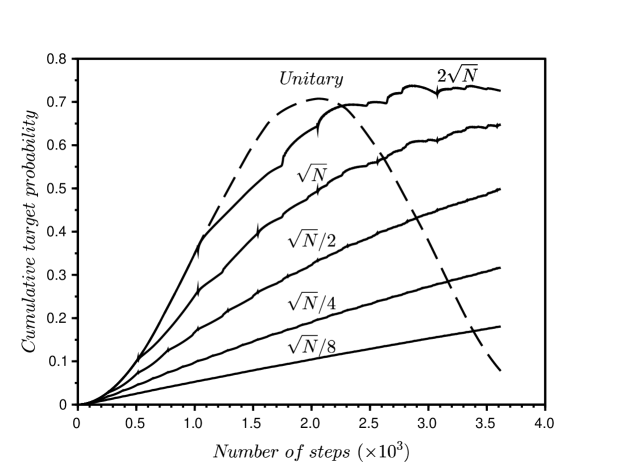
Figure 4: Cumulative target probability in $IMA_{T}$ algorithm ($\delta=\arccos\left(1/\sqrt{\log{N}}\right)$) for $N=2^{18}$ and $l=2\sqrt{N},\sqrt{N},\sqrt{N}/2,\sqrt{N}/4,\sqrt{N}/8$ and unitary case(dash line)

On the other hand, when a different $\delta$ is considered, as in the $IMA_{\pi/4}$ algorithm, the cumulative probability can be improved, depending on time lapse $l$ used. In order to get symmetric operators (1), in the following numerical studies a $\delta=\pi/4$ is chosen.

The target probability in the unitary walk (for any $\delta$) can be approximated by a harmonic oscillationTulsi_2008 . As expected, when a measurement is performed on the control qubit, the state loses coherence due to the fact it is strongly correlated with the rest of the state. This fact, combined with the effect of stopping the algorithm for a zero measurement at the control qubit, causes the target probability $P_{t}$ to go near zero, similarly to energy in a damped harmonic oscillator (see Fig. (5)).

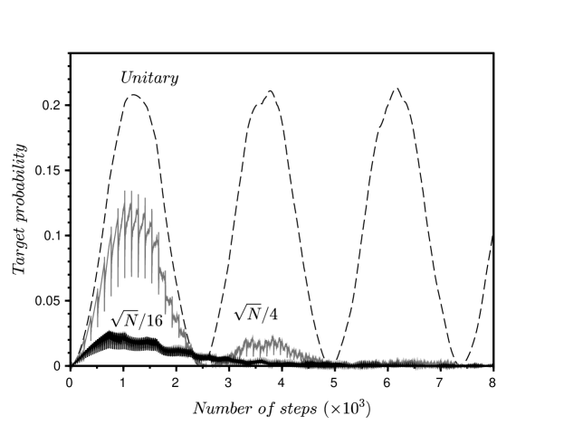
Figure 5: Target probability on $IMA_{\pi/4}$ algorithm ($\delta=\pi/4$) with $N=2^{18}$. For time lapses: $l=\sqrt{N}/4$ (gray), $l=\sqrt{N}/16$ (black), and the unitary evolution (dashed line).

The latter makes the probability $P_{c}$ tend to constant value for long times, as shown in Fig. (6).

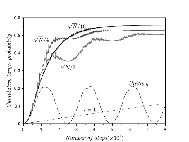
Figure 6: Cumulative target probability on $IMA_{\pi/4}$ algorithm ($\delta=\pi/4$) with $N=2^{18}$. For time lapses: $l=\sqrt{N}/2$ (light gray), $l=\sqrt{N}/4$ (gray), $l=\sqrt{N}/16$ (black), $l=1$ (dotted line) and the unitary evolution (dashed line).

IV.1 Correlations

In recent years some authors studied the behavior between probabilities and state correlations in quantum search algorithmsCui_2010 . In this section we analyze the relation of $P_{c}$ and $P_{t}$ with some correlation measures, as the bipartite Mutual InformationVedral_2002 ($MI$) and the multipartite cumulative correlationFonseca_2014 ($CCM$). A major advantage of these correlations is that they do not need nonlinear optimization methods. This is important because of the large number of states used in our quantum search.

In $IMA$ the state space have natural partitions, composed by the control, the coin and the position. The bipartite correlation that comes from partitioning the space in $\mathcal{H}_{control}\otimes\mathcal{H}_{coin+position}$, called $MI_{ctr\otimes(c,p)}$, is given by

$$MI_{ctr\otimes(c,p)}(\rho)=-S(\rho)+S(\rho_{ctr})+S(\rho_{c,p})$$ (22)

where $\rho$ is the total density matrix of the state, $\rho_{ctr}$ is the reduced matrix of the control qubit, $\rho_{c,p}$ is the reduced matrix of the coin-position subspace, and $S$ the Von Neumann entropy.

Other bipartite correlations are: $MI_{(ctr,c)\otimes p}$ and $MI_{(p,ctr)\otimes c}$. In these cases the state $\rho$ is always pure, so $S(\rho)=0$. Therefore, the distinction between classical and quantum parts is irrelevant, and can be considered a measure of entanglementZhang_2012 .

We consider also others bipartite correlations of mixed states, as the $MI$ between the coin and the position ($MI_{c\otimes p}$), the control and the coin ($MI_{ctr\otimes c}$), and the control and the position ($MI_{ctr\otimes p}$). For example, the $MI_{c\otimes p}$ is given by

$$MI_{c\otimes p}(\rho)=-S(\rho_{c,p})+S(\rho_{c})+S(\rho_{p}),$$ (23)

were, in this case, $S(\rho_{c,p})\neq 0$.

IV.2 $P_{t}$ versus correlations

Due to the explicit correlation imposed by the oracle (1), the target probability $P_{t}$ shows a similar behavior as the correlations that isolate the control qubit: $MI_{ctr\otimes(c,p)}$, $MI_{ctr\otimes p}$ and $MI_{ctr\otimes c}$ (see Fig. (7)). These correlations must be zero immediately after the measurement of the control qubit as seen in the detail in Fig. (7). The fluctuations that appear after the measurement, both in the probability and the correlation, are due to secondary waves commonly related to quantum walksKnight_2003 . As fluctuations become smaller with increasing $N$, and with the intention of assessing the average behavior, the curves are smoothed by taking a suitable average for each case.

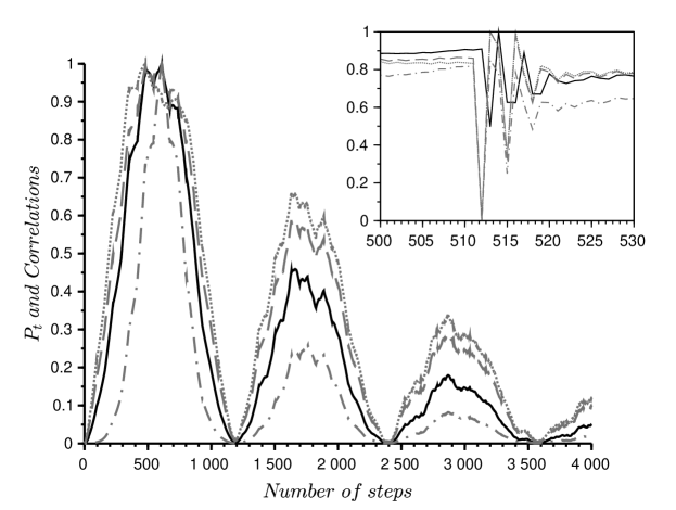
Figure 7: Target probability $P_{t}$(black solid) compared with correlations: $MI_{ctr\otimes(c,p)}$(dashed gray), $MI_{ctr\otimes p}$(dotted gray) and $MI_{ctr\otimes c}$(dash dotted gray), for $N=2^{16}$ and $l=\sqrt{N}/2$, all normalized and smoothed. In detail, original curves without smoothing.

Figure (8) shows the evolution of the probability of obtaining the state $|1\rangle$ in the control qubit. As can be observed, with the growth of the number of steps, the control qubit $\rho_{(ctr)}$ tends to be very near to a pure $|1\rangle$ state, and $S(\rho_{(ctr)})\approx 0$.

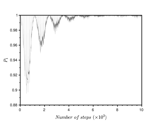
Figure 8: Probability of the control qubit being in state $|1\rangle$. Case for $N=2^{16}$ and $l=\sqrt{N}/2$.

Considering equation (22) and that $\rho$ is a pure state,

$$MI_{ctr\otimes(c,p)}=2S\left(\rho_{ctr}\right)\approx 0.$$ (24)

In the case of the others correlations, we have

$$MI_{ctr\otimes p} = -S\left(\rho_{ctr,p}\right)+S\left(\rho_{ctr}\right)+S\left(\rho_{p}\right),$$ (25)

$$\approx -S\left(\rho_{ctr,p}\right)+S\left(\rho_{p}\right),$$

$$\approx 0.$$

Similarly, $MI_{ctr\otimes c}\approx 0$.

For a constant $l=1$, the bipartite correlations $MI_{ctr\otimes(c,p)}$, $MI_{ctr\otimes p}$ and $MI_{ctr\otimes c}$, are always zero, and correspondingly $P_{t}$ is very low and $P_{c}$ is almost linear (Figure (6)).

IV.3 $P_{c}$ versus correlations

On the other hand, the cumulative probability $P_{c}$ has a similar behavior compared to the correlations $MI_{(p,ctr)\otimes c}$, $MI_{(ctr,c)\otimes p}$ and $MI_{c\otimes p}$. These correlations oscillate, until they stabilize ($\pm 5\%$) approximated in $5k_{max}$ steps, as can be seen in Fig. (9). This behavior is expected, since with the increased number of steps, the influence of the control qubit becomes negligible (24). Therefore, for a large number of steps

$$MI_{(p,ctr)\otimes c} = -S\left(\rho\right)+S\left(\rho_{p,ctr}\right)+S\left(\rho_{c}\right)\approx S\left(\rho_{p}\right)+S\left(\rho_{c}\right),$$ (26)

$$MI_{(ctr,c)\otimes p} = -S\left(\rho\right)+S\left(\rho_{ctr,c}\right)+S\left(\rho_{p}\right)\approx S\left(\rho_{p}\right)+S\left(\rho_{c}\right),$$ (27)

$$MI_{c\otimes p} = -S\left(\rho_{c,p}\right)+S\left(\rho_{p}\right)+S\left(\rho_{c}\right)=-S\left(\rho_{ctr}\right)+S\left(\rho_{p}\right)+S\left(\rho_{c}\right)$$ (28)

$$\approx S\left(\rho_{p}\right)+S\left(\rho_{c}\right).$$

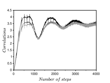
(a) Correlations $MI_{(p,ctr)\otimes c}$ (dark gray), $MI_{(ctr,c)\otimes}$ (black) and $MI_{c\otimes p}$ (light gray). As the number of steps grows all correlations tends to be similar.

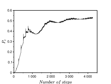
(b) Cumulative target probability $P_{c}$

Figure 9: Cumulative target probability $P_{c}$ compared with correlations, for $N=2^{16}$ and $l=\sqrt{N}/2$.

For unitary evolutions these correlations have also similar behaviors. They have a relative minimum where the target probability reaches a maximum, as shown in Fig. (10). This effect is caused by the convergence of the position subspace towards the target position, becoming less correlated with the rest of the state around the step of maximum probability.

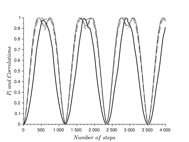
Figure 10: Target probability $P_{t}$ compared with Correlations: $MI_{(p,ctr)\otimes c}$(dashed gray), $MI_{(ctr,c)\otimes p}$(dash dotted gray) and $MI_{c\otimes p}$(dotted black), for $N=2^{16}$ for unitary evolution all normalized.

The same phenomena has been observed in Grover’s search algorithmCui_2010 . It has been found that ConcurrenceWootters_2001 works as an indicator for the increasing rate of probability. Unlike the unitary $IMA_{\pi/4}$, in Grover’s algorithm the target probability increases to values near to one, and at the same time the correlation decreases approximately to zeroGrover_1996 .

IV.4 Total steps versus correlations

In order to obtain an arbitrary search probability $P$, i. e. near $1$, amplification needs to be applied. As mentioned in section III, due to intermediate measurements, we apply classical amplification. Given an experiment with probability of success $P_{0}$, the total number of independent repetitions $R$ needed to obtain an arbitrary probability $P$ can be calculated as (geometric distribution)

$$P = 1-(1-P_{0})^{R},$$

$$\Rightarrow R = \frac{\log{1-P}}{\log{1-P_{0}}}$$ (29)

Hence, given that each experiment has $k_{max}$ steps and a probability of success equal to $P_{c}$, the total number of steps is

$$TS=k_{max}\frac{\log(1-P)}{\log(1-P_{c})}.$$ (30)

In the unitary algorithm $k_{max}$ is chosen as $(\pi/4)\sqrt{(}N\log(N))$. In the case of $IMA$ algorithm, it is interesting to compare the results for the former choice and the optimal $k_{max}$ obtained by minimization of $TS$.

An interesting fact is that correlation in the $\mathcal{H}_{ctr\otimes c}$ subspace can be used as an indicator that approximates the point of optimal step $k_{max}$. Figure (11) shows the curves $MI_{ctr\otimes c}$, $CCM(\rho_{ctr,c})$ and $e$, where

$$e(k)=\frac{1}{k}\frac{\log(1-P_{c})}{\log(1-P)},$$ (31)

being $TS=1/e(k_{max})$. Multipartite correlations are commonly generalizations of bipartite ones, and have been used in several contextsVedral_2002 ; Rulli_2011 . Multipartite correlation $CCM$Fonseca_2014 is a measure that considers, in a cumulative manner, all the bipartitions of the state space.

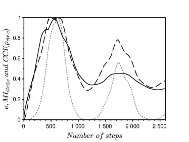
(a) $l=\sqrt{N}$

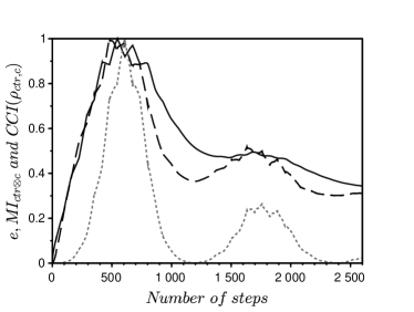
(b) $l=\sqrt{N}/2$

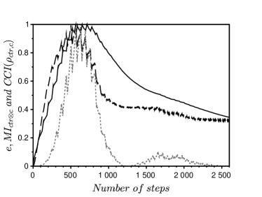
(c) $l=\sqrt{N}/4$

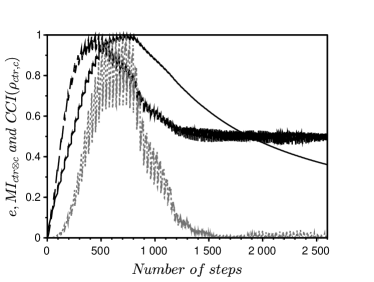
(d) $l=\sqrt{N}/8$

Figure 11: Correlations $CCM$(dashed black) and $MI_{ctr\otimes c}$(dotted gray), and $e(k)$, Eq. (31), versus number of steps. Curves smoothed and normalized.

Finally, Fig. (12) shows both $e(k_{max})$ and $MI_{c\otimes p}(k_{max})$ as a function of time lapse $l$, each evaluated for a fixed $N$ ($N=2^{14}$ and $N=2^{16}$) and two different $k_{max}$ (optimal and $\pi/4\sqrt{N\log{N}}$). All curves present a maximum for $l=\sqrt{N}/4$ ($m=4$). Interestingly, both the maximum of correlations and $e(k)$ occur for the same value of $l=\sqrt{N}/4$.

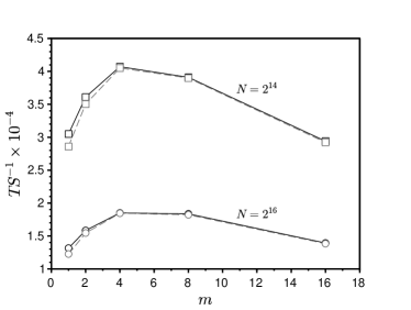
(a) Total number of steps (expressed as $TS^{-1}$) as a function of $l$ ($m=\sqrt{N}/l$).

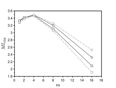
(b) Correlation $MI_{c\otimes p}$ as a function of $l$ ($m=\sqrt{N}/l$).

Figure 12: Comparison between $TS^{-1}$ ($e(k_{max})$) and the correlations $MI_{c\otimes p}$, for fixed $N=2^{14}$(square), $N=2^{16}$(circle). Both $TS$ and the correlation are smoothed and evaluated at the optimal $k_{max}$(dashed gray), and $k_{max}=\pi/4\sqrt{N\log{N}}$ (black).

As can be observed, the results for the optimal $k_{max}$ and the standard $\pi/4\sqrt{N\log{N}}$ are very similar, which justifies the usage of the latter.

V Estimating the algorithm’s order

The order of this type of search algorithm can be estimated by the number of steps needed to obtain a target probability of order one. $AKR$ algorithm, with quantum amplitude amplificationBrassard_2002 , has order $O(\sqrt{N}\log{N})$. If classical amplitude amplification is used, the order becomes $O(\sqrt{N}\log^{\frac{3}{2}}N)$Aaronson_2003 .

In Tulsi’s algorithm, the target probability is around $\frac{1}{\cos{\delta}\sqrt{\log N}}$, resulting in an order of $O(\sqrt{N\log N})$. For unitary $IMA_{\pi/4}$ (Tulsi with $\delta=\pi/4$) using classical amplitude amplification, the order is the same as for $AKR$, i.e. $O(\sqrt{N}\log^{3/2}{N})$.

Motivated by the results of the previous section, where it was observed that the total number of steps $TS$ varies with time lapse $l$, in this section we estimate bounds for the order of the $IMA_{\pi/4}$ algorithm for some $l$ values.

Figure (13) shows the total number of steps $TS$ as a function of $N$ , for some $l$ values. As can be seen in Figure (13.c), when divided by $N$, the curve corresponding to the $l=1$ case is the only curve that converges to a constant value. In this case the algorithm has the same order as the classical brute-force search algorithm. Other curves show a better order than classical. Due to computational limitations to obtain results for large values of $N$, it is very hard to perform good nonlinear regressions to fit the order. Instead, we estimate ranges for the order depending on $l$, dividing the curves in Figure (13.b) by functions of type

$$\beta\sqrt{N}(\log{N})^{\alpha},$$ (32)

for some $\alpha$. Figure (14) shows the results for $\alpha$ equal to: $1.5$, $1.25$, $0.9$ and $0.6$.

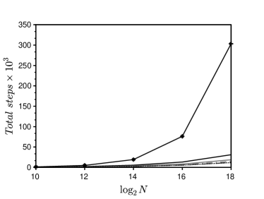
(a) Total steps $TS$ as a function of $N$. Solid black curve with asterisk for the case $l=1$ (measurement in all steps). Details for the others curves in Figure b.

(b) Detail for the unitary case (solid black), $l=\sqrt{N}$ (solid gray), $l=\sqrt{N}/2$ (dash dotted gray), $l=\sqrt{N}/4$ (dashed gray) and $l=\sqrt{N}/8$ (dotted black).

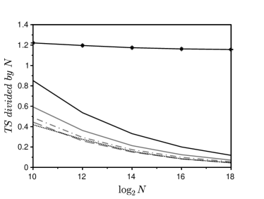
(c) $TS$ divided by $N$. The curve for $l=1$ is the only that converges to a constant value

Figure 13: Total steps $TS$ as a function of $N$. Curves for the unitary case and $l=1,\sqrt{N},\sqrt{N}/2,\sqrt{N}/4,$ and $\sqrt{N}/8$.

(a) $TS$ divided by $\sqrt{N}(\log{N})^{1.5}$

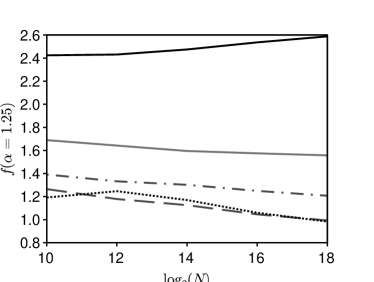
(b) $TS$ divided by $\sqrt{N}(\log{N})^{1.25}$

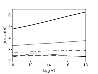
(c) $TS$ divided by $\sqrt{N}(\log{N})^{0.9}$

(d) $TS$ divided by $\sqrt{N}(\log{N})^{0.6}$

Figure 14: Total steps $TS$ divided by fitting curve $\left(f(\alpha)=\frac{TS}{\sqrt{N}(\log{N})^{\alpha}}\right)$. Unitary case (solid black), $l=\sqrt{N}$ (solid gray), $l=\sqrt{N}/2$ (dash dotted gray), $l=\sqrt{N}/4$ (dashed gray) and $l=\sqrt{N}/8$ (dotted black).

It can be observed that:

• The curve corresponding to the unitary algorithm tends to be constant when divided by Eq. (32) with $\alpha=1.5$ (Figure (14).(a)), as expected.

• For $l=\sqrt{N}$ and $\sqrt{N}/2$ the order is in the range $\alpha\in\left[0.9,1.25\right]$, as can be appreciated in Figures (14).(c) and (14).(b).

• In the cases $l=\sqrt{N}/4$ and $\sqrt{N}/8$, Figures (14).(c) and (14).(d) shows that the order is in the range $\alpha\in\left[0.6,0.9\right]$.

VI Conclusions

In this paper a modified Tulsi’s algorithm with intermediate partial measurements of the control qubit($IMA_{\pi/4}$), is presented.

The target probability $P_{t}$, and some correlations (Section IV.2), behave similarly to energy of a damped harmonic oscillator, where time lapse $l$ works as a decoherence parameter, going from quantum to classical.

The performance of the algorithm also has a strong relation with some correlations. The maxima in the $MI_{ctr\otimes c}$ and $CCM$ curves indicate the optimal step to stop the algorithm, when classical amplification is considered. What is more, as it can be observed from Figures (11) and (12), when these maxima have better coincidence ($l=\sqrt{N}/4$) the algorithm $IMA_{\pi/4}$ has minimal total steps $TS$.

For some values of $l$, the order estimated shows an improvement with respect to the unitary case. However, a numerical approach to find the order is limited by computational power. This fact motivates, as a future work, the search of analytical approaches to this problem.

This study, with partial intermediate measurements in quantum search algorithms, is a start point to analyze possible improvements of other quantum algorithms using one, or several, control qubits.

References

- [1] M. Van den Nest. Computation with little entanglement. Phys. Rev. Lett., 110:060504, 2013.
- [2] Jian Cui and Heng Fan. Correlations in grover search. J. Phys. A: Math. Theor., 43:04530, 2010.
- [3] M. A. Nielsen and I. L. Chuang. Quantum computation and quantum information. Cambridge Univ. Press, 2000.
- [4] A. Romanelli, R. Siri, G. Abal, A. Auyuanet, and R. Donangelo. Decoherence in the quantum walk on the line. Physica A: Statistical Mechanics and its Applications, Volume 347:137–152, 2005.
- [5] P. J. Salas. Noise effect on grover algorithm. The European Physical Journal D, 46:365–373, 2008.
- [6] G. Abal, R. Donangelo, F.L. Marquezino, A.C. Oliveira, and R. Portugal. Decoherence in search algorithms. In Proceedings of the XXIX Brazilian Computer Society Congress (SEMISH), pages 293–306, 2009.
- [7] R. Srikanth, Subhashish Banerjee, and C. M. Chandrashekar. Quantumness in a decoherent quantum walk using measurement-induced disturbance. Phys. Rev. A., 81:062123, 2010.
- [8] P. Gawron, J. Klamka, and R. Winiarczyk. Noise effects in the quantum search algorithm from the computational complexity point of view. Int. J. Appl. Math. Comput. Sci., 22, No. 2:493–499, 2012.
- [9] T. Tulsi, L. Grover, and A. Patel. A new algorithm for fixed point quantum search. Quantum Information and Computation, 26:483–494, 2006.
- [10] O. Maloyer and V. Kendon. Decoherence vs entanglement in coined quantum walks. New J. Phys., 9:87, 2007.
- [11] Viv Kendon. Decoherence in quantum walks. Mathematical Structures in Computer Science, 17 Issue 6:1169–1220, 2007.
- [12] Salvador Elias Venegas-Andraca. Quantum walks: a comprehensive review. Quantum Information Processing, 11:1015–1106, 2012.
- [13] Renato Portugal. Quantum Walks and Search Algorithms. Springer, 2013.
- [14] Robert Raussendorf, Daniel E. Browne, and Hans J. Briegel. Measurement-based quantum computation on cluster states,. Phys. Rev. A, 68:022312, 2003.
- [15] Avatar Tulsi. Faster quantum-walk algorithm for the two-dimensional spatial search. Phys. Rev. A, 78:012310, 2008.
- [16] L.K. Grover. A fast quantum mechanical algorithm for database search. In Proceedings, 28th Annual ACM Symposium on the Theory of Computing p. 212, 1996.
- [17] A. Ambainis, J. Kempe, and A. Rivosh. Coins make quantum walks faster. In Proceedings of SODA 2005, pp. 1099-1108, 2005.
- [18] In this article the subscripts , and , indicate the control, coin and position subspaces, respectively.
- [19] P. Benioff. Space searches with a quantum robot. In CONTEMPORARY MATHEMATICS AMS Contemporary Math Series: Quantum Computation and Information, volume Vol 305, 2002.
- [20] The examples were performed using QuantumLab[29], a quantum simulator toolbox for Scilab.
- [21] V. Vedral. The role of relative entropy in quantum information theory. Rev. Mod. Phys, 74:197–234, 2002.
- [22] A. L. Fonseca De Oliveira, E. Buksman, and J. G. Lopez de Lacalle. Cumulative measure of correlation for multipartite quantum states. Int. J. Mod. Phys. B, 28:1450050, 2014.
- [23] Jian-Song Zhang and Ai-Xi Chen. Review of quantum discord in bipartite and multipartite systems. Quant. Phys. Lett., Vol. 1 No. 2:69–77, 2012.
- [24] Peter L. Knight, Eugenio Rold n, and J. E. Sipe. Quantum walk on the line as an interference phenomenon. Phys. Rev. A, 68:020301, 2003.
- [25] WILLIAM K. WOOTTERS. Entanglement of formation and concurrence. Quantum Information and Computation,, Vol. 1, No. 1:27– 44, 2001.
- [26] C. C. Rulli and M. S. Sarandy. Global quantum discord in multipartite systems. Phys. Rev. A, 84:042109, 2011.
- [27] Gilles Brassard, Peter H yer, Michele Mosca, and Alain Tapp. Quantum amplitude amplification and estimation. Contemporary Mathematics, 305:53, 2002.
- [28] S. Aaronson and A. Ambainis. Quantum search of spatial structures. In Proceedings of the 44th Annual IEEE Symposium on Foundations of Computer Science, 2003.
- [29] A. L. F. de Oliveira and E. Buksman. Simulacion de errores cuanticos en el ambiente scilab. Technical report, Universidad ORT Uruguay, 2007.