A tunable, nonlinear Hong-Ou-Mandel interferometer

Abstract

We investigate the two-photon scattering properties of a Jaynes-Cummings (JC) nonlinearity consisting of a two-level system (qubit) interacting with a single mode cavity, which is coupled to two waveguides, each containing a single incident photon wave packet initially. In this scattering setup, we study the interplay between the Hong-Ou-Mandel effect arising due to quantum interference and effective photon-photon interactions induced by the presence of the qubit. We calculate the two-photon scattering matrix of this system analytically and identify signatures of interference and interaction in the second order auto- and cross-correlation functions of the scattered photons. In the dispersive regime, when qubit and cavity are far detuned from each other, we find that the JC nonlinearity can be used as an almost linear, in-situ tunable beam splitter giving rise to ideal Hong-Ou-Mandel interference, generating a highly path-entangled two-photon NOON state of the scattered photons. The latter manifests itself in strongly suppressed waveguide cross-correlations and Poissonian photon number statistics in each waveguide. If the two-level system and the cavity are on resonance, the JC nonlinearity strongly modifies the ideal HOM conditions leading to a smaller degree of path entanglement and sub-poissonian photon number statistics. In the latter regime, we find that photon blockade is associated with bunched auto-correlations in both waveguides, while a two-polariton resonance can lead to bunched as well as anti-bunched correlations.

I Introduction

The Hong-Ou-Mandel (HOM) effect hong1987 lies at the heart of linear optical quantum computing knill2001 ; kimble2008 and is utilized to test the degree of indistinguishability of photons as well as the quality of single photon sources. Conventionally, the HOM effect is demonstrated as a two-photon interference effect at a linear 50/50 beam splitter: when two indistinguishable photon wave packets impinge on the beam splitter from two different waveguides, they form an entangled two-photon NOON state with both photons in the same output waveguide which produces a characteristic dip in the coincidence probability of finding photons in both waveguides simultaneously. This destructive interference is complete only for indistinguishable photons with equal energy and zero time delay. Any deviation from the ideal conditions leads to a diminishing of the dip, which thus constitutes a measure for indistinguishability.

The HOM effect has been demonstrated experimentally using parametric down conversion hong1987 and pulsed single photon sources operating at optical frequencies santori2002 ; deriedmatten2003 ; legero2004 ; beugnon2006 ; maunz2007 . Recently, the HOM effect has attracted new attention in the context of waveguide and circuit QED blais2004 ; wallraff2004 ; longo2011 ; pletyukhov2014 , where it was demonstrated with unprecedented precision for microwave photons as well lang2013 ; woolley2013 , using recently developed microwave single photon sources and beam splitters. This development paves the way for all-integrated linear optical quantum computing at microwave frequencies.

In all experiments so far, the central element of the HOM effect, i.e., a $50/50$ beam splitter, was based on a linear and static device, whose single-photon transmission and reflection probabilities (which are constant over a broad range of frequencies) are fixed by the manufacturing process. From an experimental point of view it would be desirable to also utilize beam splitters with in-situ tunable reflection and transmission probabilities.

Figure 1: Schematic of the scattering setup with a qubit-cavity system interacting via the light-matter interaction strength $g$ and directly connected to two transmission lines giving rise to a cavity decay rate $\kappa=2\pi g_{\mathrm{w}}^{2}$. We consider two single-photon wave packets with spatial width $v/\xi$ impinging on the cavity from two different directions, e.g., emitted by two independent single photon sources houck:07 ; lang:11 .

In this paper we study theoretically two-photon scattering at a Jaynes-Cummings nonlinearity shi:11 , i.e., a coupled qubit-cavity system, connected directly to two transmission lines. Such a scattering setup is readily realizable using state of the art circuit QED technology. Hereby, the transition frequency of the two-level system (qubit) is a flux-tunable parameter, which allows to energetically shift the effective single-photon resonances of the qubit-cavity system. Due to the finite width of the resonances induced by the coupling to the transmission lines, one can fine-tune the single photon transmission and reflection probabilities of the scattering target. The Jaynes-Cummings nonlinearity may thus act as an in-situ tunable beam splitter in a waveguide QED setup. This tunable beam splitter works best for energies of the incoming photons with a bandwidth $\xi$ smaller than the cavity decay rate $\kappa$. In circuit QED, this condition can be satisfied by using a driven qubit-cavity system as a single photon source houck:07 ; lang:11 which couples more weakly to the waveguide (leading to sharp wave packets) than the beam splitter cavity.

In addition, the two-level system introduces a nonlinearity into the system, which may modify the ideal HOM conditions. Here, we investigate in detail the interplay between the two-photon interference and effective photon-photon interactions in a Jaynes-Cummings system. For this purpose, we utilize an analytic scattering matrix approach recently developed for a two-level system embedded in a chiral photonic waveguide pletyukhov2012 . Based on this analytic approach, we derive the exact two-photon scattering matrix of the proposed setup and identify experimentally measurable signatures of the HOM effect and effective photon-photon interactions in the second-order cross- and auto-correlation functions of the two output modes. In the dispersive regime, i.e., when the two-level system and the cavity are far detuned from each other, the Jaynes-Cummings nonlinearity gives rise to a qubit-like and a cavity-like scattering resonance. In the vicinity of these resonances, the two-photon scattering matrix of a qubit and a Kerr-like nonlinearity, previously studied in the context of the HOM effect longo2011 , are derived as limiting cases.

II Model

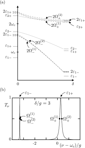
Figure 2: (a) Energy level diagram of the Jaynes-Cummings Hamiltonian showing the upper/lower one- and two-polariton resonances $\varepsilon_{1\sigma}$ and $\varepsilon_{2\sigma}$ defined in Eq. (7) for zero detuning ($\delta=0$) on the left and for large positive detuning ($\delta>0$) on the right. Dashed lines correspond to the two-photon energies $2\Omega^{(1,2)}_{\sigma}$ defined in Eq. (15) leading to the ideal HOM effect for sharp wave packets with $\xi\rightarrow 0$. Dotted lines correspond to the two-polariton energies $\varepsilon_{2\sigma}$ and $2\varepsilon_{1\sigma}$ as a function of detuning $\delta$. Their difference measures the nonlinearity in the Jaynes-Cummings spectrum $U=\varepsilon_{2\sigma}-2\varepsilon_{1\sigma}$. (b) The single-photon transmission probability (i.e., transmission to the other waveguide) $T_{\nu}=|t_{\nu}|^{2}$ exhibits two Lorentzian resonances located approximately around the two-level system frequency $\omega_{q}$ and the cavity frequency $\omega_{c}$ in the dispersive regime with $|\delta|=|\omega_{c}-\omega_{q}|\gg g$. The energies $\Omega_{\sigma}^{(1,2)}$ correspond to ideal HOM conditions with $T_{\nu}=R_{\nu}=1/2$ (where $R_{\nu}=|r_{\nu}|^{2}$ denotes the reflection probability and we have chosen $\kappa/g=0.1$).

Figure 1 shows the scattering setup considered in this paper. The total Hamiltonian of this system is given by

$$H=H_{\rm\scriptscriptstyle JC}+H_{\rm w}+V$$ (1)

with the Jaynes-Cummings Hamiltonian

$$H_{\rm\scriptscriptstyle JC}=\omega_{c}b^{\dagger}b+\omega_{q}\sigma^{+}\sigma^{-}+g(b^{\dagger}\sigma^{-}+b\sigma^{+})$$ (2)

describing the coupled qubit-cavity system, we set $\hbar=1$. The Hamiltonian $H_{\rm w}$ of the transmission lines describes photons in chiral states (see Fig. 1) with linear dispersion $\nu=vk$ with wavevector $k>0$ and velocity $v$, i.e.,

$$H_{\rm w}=\sum_{i=1,2}\int d\nu\,\nu\,a_{i\nu}^{\dagger}a_{i\nu}\,,$$ (3)

which linearly couple to the scatterer via

$$V=g_{\mathrm{w}}\sum_{i=1,2}\int d\nu\,(b^{\dagger}a_{i\nu}+\text{h.c.})\,.$$ (4)

Here, we have introduced the cavity photon operator $b$ and the operators $a_{i\nu}$ describing photons with energy $\nu$ in waveguide $i$. The two-level system, described by the raising/lowering operators for a two-level system $\sigma^{\pm}$, introduces a nonlinearity into the system due to the light-matter coupling $\sim g$. In our model, we neglect a coupling of the two-level system to other modes of the system and environment, because the associated spontaneous emission rates can be engineered to be several orders of magnitude smaller than the qubit-cavity coupling $g$ and cavity decay rate $\kappa=2\pi g_{\mathrm{w}}^{2}$ to the leads (for typical parameter values in circuit QED systems, see Ref. schmidt:13 ).

The scattering resonances are determined by the eigenstates of the Jaynes-Cummings Hamiltonian: The ground state $|\psi_{0}\rangle=|0,\downarrow\rangle$ consists of zero photons in the cavity and the two-level system in its ground state with energy $\varepsilon_{0}=0$. The excited states ($n>0$) are

$$|\psi_{n+}\rangle =\cos\frac{\theta_{n}}{2}|n-1,\uparrow\rangle+\sin\frac{\theta_{n}}{2}|n,\downarrow\rangle,$$ (5)

$$|\psi_{n-}\rangle =-\sin\frac{\theta_{n}}{2}|n-1,\uparrow\rangle+\cos\frac{\theta_{n}}{2}|n,\downarrow\rangle,$$ (6)

with the angle $\tan\theta_{n}=-2g\sqrt{n}/\delta$ and the detuning $\delta=\omega_{c}-\omega_{q}$. They correspond to $n$ excitations, i.e., polariton quasi-particles, which form a superposition of the state $|n,\downarrow\rangle$ with $n$ photons in the cavity and the two-level system in the ground state and the state $|n-1,\uparrow\rangle$ with $(n-1)$ photons in the cavity and the two-level system in the excited state. The corresponding energies are given by

$$\varepsilon_{n\pm}=n\omega_{c}-\delta/2\pm\sqrt{(\delta/2)^{2}+ng^{2}}.$$ (7)

The JC eigenenergies give rise to single-photon scattering resonances with Lorentzian peaks at $\varepsilon_{1\pm}$ as a function of incoming photon energy. Due to the coupling to the waveguide, the cavity states also attain a finite lifetime $\sim 1/\kappa$ with $\kappa=2\pi g_{\mathrm{w}}^{2}$. In the next section, we will derive explicit expressions for the single-photon and two-photon scattering matrix of this system.

III Scattering formalism

We consider the generic situation, where an initial one- or two-photon state $|\psi_{\rm in}\rangle$ is prepared inside the wave-guides at $t_{\rm in}=-\infty$, interacts (scatters) at the Jaynes-Cummings nonlinearity and is observed as the out-going state $|\psi_{\rm out}\rangle$ in a photon detector at $t_{\rm out}=+\infty$. The relation between the initial and the scattered state is given by the $S$-matrix, i.e.,

$$|\psi_{\rm out}\rangle=S|\psi_{\rm in}\rangle\quad{\rm with}\quad S=\mathcal{T}\exp\bigl{[}-i\int_{-\infty}^{\infty}V(t)dt\bigr{]}\,.$$ (8)

Here, we have written the coupling Hamiltonian in the interaction representation, i.e., $V(t)=\exp(iH_{0}t)V\exp(-iH_{0}t)$ with $H_{0}=H_{\rm\scriptscriptstyle JC}+H_{\rm w}$.

In the following, we will need the one-photon $S$-matrix (for the scattering at an empty cavity/qubit, i.e., void of excitations) written in a Fock state basis as

$$P_{0}S^{(1)}P_{0}=P_{0}\sumint S^{ij}_{\nu^{\prime}\nu}\,a^{\dagger}_{i\nu^{\prime}}a_{j\nu}$$ (9)

with matrix elements $S_{\nu^{\prime}\nu}^{ij}=\langle 0|a_{i\nu^{\prime}}S^{(1)}a^{\dagger}_{j\nu}|0\rangle$. Here $|0\rangle\equiv|\psi_{0}\rangle\otimes|0\rangle_{\mathrm{w}}$ is the state void of excitations, i.e., no photons in cavity and waveguide, and the two-level system residing in its ground state; $P_{0}=|\psi_{0}\rangle\langle\psi_{0}|$ is the projector onto the dark state of the cavity, i.e., $|\psi_{0}\rangle=|0,\downarrow\rangle$. The symbol $\sumint=\sum_{ij}\int_{\nu^{\prime}\nu}$ denotes summation (integration) over all arabic (greek) indices. Similarly, the two-photon scattering matrix is defined as

$$P_{0}S^{(2)}P_{0}=\frac{P_{0}}{4}\sumint_{1}\sumint_{2}S^{i_{1}i_{2}j_{1}j_{2}}_{\nu^{\prime}_{1}\nu^{\prime}_{2}\nu_{1}\nu_{2}}\,a^{\dagger}_{i_{1}\nu^{\prime}_{1}}a^{\dagger}_{i_{2}\nu^{\prime}_{2}}a_{j_{1}\nu_{1}}a_{j_{2}\nu_{2}},$$ (10)

with $S^{i_{1}i_{2}j_{1}j_{2}}_{\nu^{\prime}_{1}\nu^{\prime}_{2}\nu_{1}\nu_{2}}=\langle 0|a_{i_{2}\nu^{\prime}_{2}}a_{i_{1}\nu^{\prime}_{1}}S^{(2)}a^{\dagger}_{j_{1}\nu_{1}}a^{\dagger}_{j_{2}\nu_{2}}|0\rangle$.

Both, single- and two-photon scattering matrix elements are calculated in App. A by making use of the formalism developed in Ref. pletyukhov2012, . For the single photon matrix elements in (9) we obtain

$$S^{11}_{\nu^{\prime}\nu} =S^{22}_{\nu^{\prime}\nu}=r_{\nu}\delta(\nu^{\prime}-\nu),$$ (11)

$$S^{12}_{\nu^{\prime}\nu} =S^{21}_{\nu^{\prime}\nu}=t_{\nu}\delta(\nu^{\prime}-\nu),$$ (12)

with the reflection (= scattering to the same waveguide) amplitude

$$r_{\nu}=\frac{(\nu-\omega_{q})(\nu-\omega_{c})-g^{2}}{(\nu-\omega_{q})(\nu-\omega_{c}+i\kappa)-g^{2}}$$ (13)

and the transmission (= scattering to the other waveguide) amplitude

$$t_{\nu}=\frac{-i\kappa(\nu-\omega_{q})}{(\nu-\omega_{q})(\nu-\omega_{c}+i\kappa)-g^{2}}\,.$$ (14)

The reflection amplitude vanishes for $\nu=\varepsilon_{1,\pm}$, giving rise to resonances in transmission, see Fig. 2(b). The one-photon resonance energies and widths are determined by $\tilde{\varepsilon}_{1,\pm}$ which is obtained from $\varepsilon_{1,\pm}$, cf. Eq. (7), by replacing the cavity frequency $\omega_{c}$ by $\tilde{\omega}_{c}=\omega_{c}-i\kappa$ (and correspondingly replacing the detuning $\delta$ by $\tilde{\delta}=\delta-i\kappa$; the $n$-excitation resonances $\tilde{\varepsilon}_{n,\pm}$ are defined in the same way). For large positive detuning $\delta\gg g$, the upper polariton resonance at $\varepsilon_{1,+}$ is cavity-like with a width $\kappa$, while the lower polariton resonance at $\varepsilon_{1,-}$ is qubit-like with an effective width $\kappa g^{2}/\delta^{2}$.

In the context of the Hong-Ou-Mandel effect it is also useful to define the single-photon energies

$$\Omega^{(1,2)}_{\sigma} =\frac{1}{2}\Bigl{(}\omega_{c}+\omega_{q}\pm\kappa+\sigma\sqrt{(\delta\pm\kappa)^{2}+4g^{2}}\Bigr{)}\,,\quad\sigma=\pm\,,$$ (15)

where the single-photon transmission and reflection probabilities are equal to $1/2$, corresponding to a 50/50 beam splitter operation, see Fig. 2(b).

The two-photon scattering matrix in (10) is of the form

$$S^{i_{1}i_{2}j_{1}j_{2}}_{\nu^{\prime}_{1}\nu^{\prime}_{2}\nu_{1}\nu_{2}}=S^{i_{1}j_{1}}_{\nu^{\prime}_{1}\nu_{1}}S^{i_{2}j_{2}}_{\nu^{\prime}_{2}\nu_{2}}+S^{i_{2}j_{1}}_{\nu^{\prime}_{2}\nu_{1}}S^{i_{1}j_{2}}_{\nu^{\prime}_{1}\nu_{2}}+i\mathcal{T}^{(2)}_{\nu^{\prime}_{1}\nu^{\prime}_{2}\nu_{1}\nu_{2}}\,.$$ (16)

The first two terms describe two uncorrelated single photon scattering events as obtained from Eqs. (11) and (12). The third term on the r.h.s of Eq. (16) describes the non-trivial two-photon scattering process described by the $T$-matrix element

$$\mathcal{T}^{(2)}_{\nu^{\prime}_{1}\nu^{\prime}_{2}\nu_{1}\nu_{2}} =\delta(\nu^{\prime}_{1}+\nu^{\prime}_{2}-\nu_{1}-\nu_{2})\frac{\kappa^{2}g^{4}}{\pi}\frac{(\nu_{1}+\nu_{2}-\tilde{\varepsilon}_{1,+}-\tilde{\varepsilon}_{1,-})}{\prod_{\alpha=\pm}(\nu_{1}+\nu_{2}-\tilde{\varepsilon}_{2,\alpha})}$$

$$\quad\times\frac{\prod_{\alpha=\pm}(\nu_{1}+\nu_{2}-2\tilde{\varepsilon}_{1,\alpha})}{\prod_{i=1,2}\prod_{\alpha=\pm}(\nu^{\prime}_{i}-\tilde{\varepsilon}_{1,\alpha})(\nu_{i}-\tilde{\varepsilon}_{1,\alpha})}\,.$$ (17)

Note that the $T$-matrix elements do not depend on the waveguide indices due to the symmetric coupling of the two transmission lines. The results in (9)-(III) are consistent with those derived in Ref. shi:11 (using a different approach) and enable us to calculate the wavefunction as well as photon statistics in the output modes for arbitrary incoming states containing up to two photons. In the next section we apply these results to the specific situation depicted in Fig. 1 with two single-photon wave packets approaching the cavity in different waveguides.

IV Hong-Ou-Mandel effect

The Hong-Ou-Mandel effect hong1987 is a two-particle-interference effect describing the spatial bunching of two indistinguishable photons which arrive at the same time at an ideal 50/50 beam splitter from two different incoming arms and always end up in the same outgoing arm. The effect is fundamentally related to the bosonic exchange properties of the photons. In the following, we will discuss such a Hong-Ou-Mandel (HOM) effect for two photon scattering at a JC nonlinearity. As discussed above, the single-photon scattering characteristics of a JC nonlinearity provide equal transmission and reflection probability at energies $\Omega^{(1,2)}_{\pm}$ (around the two polariton energies $\varepsilon_{1,\pm}$) such that the cavity-qubit system may act as an ideal 50/50 beam splitter. However, due to the finite width of the photon wave packets, the ideal beam splitter conditions can only be satisfied for one spectral component of the wave packets. Furthermore, the nonlinearity of the JC system induced by the coupling of the photons to the two-level system modifies the two-photon scattering properties compared to a linear 50/50 beam splitter. Both finite wave packet width and nonlinearity may wash out the quantum interference leading to the HOM effect and thus will be investigated in detail in the following.

In order to investigate the HOM effect, we consider two photons incoming in different waveguides described by the (normalized) incoming state

$$|\psi_{\rm in}\rangle=\iint d\nu_{1}d\nu_{2}f^{\rm\scriptscriptstyle(1)}_{\nu_{1}}f^{\rm\scriptscriptstyle(2)}_{\nu_{2}}a^{\dagger}_{1\nu_{1}}a^{\dagger}_{2\nu_{2}}|0\rangle$$ (18)

with the function $f^{\scriptscriptstyle(i)}_{\nu}$ describing the incoming photon wave packet in lead $i=1,2$, satisfying $\int d\nu|f_{\nu}^{(i)}|^{2}=1$. The outgoing state after scattering is related to the incoming state via $|\psi_{\rm out}\rangle=S|\psi_{\rm in}\rangle$ which leads to

$$|\psi_{\rm out}\rangle =|\psi^{11}_{\rm out}\rangle+|\psi^{22}_{\rm out}\rangle+|\psi^{12}_{\rm out}\rangle$$ (19)

$$=\iint d\nu_{1}d\nu_{2}f^{\rm\scriptscriptstyle(1)}_{\nu_{1}}f^{\rm\scriptscriptstyle(2)}_{\nu_{2}}$$

$$\qquad\times\Biggl{(}\frac{1}{2}\iint d\nu_{1}^{\prime}d\nu_{2}^{\prime}S^{11,12}_{\nu^{\prime}_{1}\nu^{\prime}_{2},\nu_{1}\nu_{2}}a^{\dagger}_{1\nu^{\prime}_{1}}a^{\dagger}_{1\nu^{\prime}_{2}}|0\rangle$$

$$\hskip 30.0pt+\frac{1}{2}\iint d\nu_{1}^{\prime}d\nu_{2}^{\prime}S^{22,12}_{\nu^{\prime}_{1}\nu^{\prime}_{2},\nu_{1}\nu_{2}}a^{\dagger}_{2\nu^{\prime}_{1}}a^{\dagger}_{2\nu^{\prime}_{2}}|0\rangle$$

$$\hskip 30.0pt+\iint d\nu_{1}^{\prime}d\nu_{2}^{\prime}S^{12,12}_{\nu^{\prime}_{1}\nu^{\prime}_{2},\nu_{1}\nu_{2}}a^{\dagger}_{1\nu^{\prime}_{1}}a^{\dagger}_{2\nu^{\prime}_{2}}|0\rangle\Biggr{)}$$

with three contributions; the first two contributions describe two photons scattered into the same waveguide and the third contribution describes the scattering into different waveguides. The HOM effect arises if the latter contribution $|\psi_{\rm out}^{12}\rangle$ vanishes. We thus define a HOM parameter

$$\gamma=\langle\psi_{\rm out}|n_{1}n_{2}|\psi_{\rm out}\rangle=\langle\psi_{\rm out}^{12}|\psi_{\rm out}^{12}\rangle\,,$$ (20)

with $n_{i}=\int d\nu a_{i\nu}^{\dagger}a_{i\nu}$ which yields the coincidence probability of finding one photon in the left and one photon in the right waveguide. Thus, $\gamma=0$, corresponds to a superposition of two states, one with both photons in the left and one with both photons in the right waveguide, i.e., a two photon entangled NOON state with respect to the waveguide degrees of freedom. Using Eq. (19), we obtain from (20)

$$\gamma =\iint d\nu_{1}^{\prime}d\nu_{2}^{\prime}\Bigl{|}\iint d\nu_{1}d\nu_{2}S^{12,12}_{\nu^{\prime}_{1}\nu^{\prime}_{2},\nu_{1}\nu_{2}}f^{\rm\scriptscriptstyle(1)}_{\nu_{1}}f^{\rm\scriptscriptstyle(2)}_{\nu_{2}}\Bigr{|}^{2}.$$ (21)

In the following, we will consider Lorentzian wave packets described by

$$f^{\scriptscriptstyle(i)}_{\nu}=\sqrt{\frac{\xi}{2\pi}}\frac{e^{-i\nu(t-t_{i})}}{\nu-\nu_{0i}+i\xi/2}$$ (22)

around energies $\nu_{0i}>0$ with width $\xi$. The times $t_{i}$ correspond to the instants when the fronts of the wave packets reach the mirrors of the cavity, such that the time delay between them is given by $\Delta t=t_{1}-t_{2}$. The integrals in Eq. (21) can be calculated analytically which results in explicit algebraic expressions for the HOM parameter, which, however, are rather lengthy and thus have been omitted here for brevity.

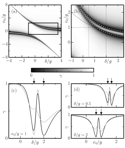
Figure 3: (a) HOM parameter $\gamma$ (defined in Eq. (20)) as a function of the detuning $\delta$ and the two-photon energy $e_{0}=\nu_{01}+\nu_{02}-2\omega_{c}$ (defined relative to the cavity frequency) for $\kappa/g=0.1$ and $\xi/\kappa=0.1$. (b) Inset in (a) (black box) together with the two photon energies depicted in Fig. 2(a) (dashed, $2\Omega_{+}^{(1,2)}$, and dotted lines, $2\varepsilon_{1,+}$ and $\varepsilon_{2,+}$, with the same notation as in Fig. 2(a)). Thin horizontal and vertical lines correspond to the cuts in (c) and (d), see below. (c) Cuts through (b) at constant two-photon energy $e_{0}/g=1$ for wave packets of width $\xi/\kappa=0.1$ (black) and $\xi/\kappa=1$ (light gray lines). The dotted lines correspond to the linear approximation (for $\xi/\kappa=0.1$), where correlation contributions due to the $T$-matrix elements in Eq. (26) are neglected. Vertical arrows correspond to the detuning for which $\nu_{01}+\nu_{02}=2\Omega^{(1,2)}_{+}$ (ideal HOM conditions). (d) Cuts through (b) at constant detuning $\delta=0.5g$ (upper panel) and $\delta=2g$ (lower panel).

Figure 3 shows the behavior of the HOM parameter $\gamma$ as obtained from the exact calculation of Eq. (21) for $\Delta t=\nobreak 0$ and equal energies of the incoming photons $\nu_{01}=\nu_{02}$. Before discussing these results in detail, it is instructive to separate uncorrelated and correlated contributions in Eq. (21). From the result for the two-photon scattering matrix in (16), we can rewrite

$$\gamma=\iint d\nu_{1}^{\prime}d\nu_{2}^{\prime}|\mathcal{A}^{12}_{\nu^{\prime}_{1},\nu^{\prime}_{2}}|^{2}$$ (23)

with

$$\mathcal{A}^{12}_{\nu^{\prime}_{1},\nu^{\prime}_{2}}=\mathcal{A}^{12,\rm lin}_{\nu^{\prime}_{1},\nu^{\prime}_{2}}+\mathcal{C}_{\nu^{\prime}_{1},\nu^{\prime}_{2}}$$ (24)

where

$$\mathcal{A}^{12,\rm lin}_{\nu^{\prime}_{1},\nu^{\prime}_{2}}=t_{\nu_{1}^{\prime}}t_{\nu_{2}^{\prime}}f^{\rm\scriptscriptstyle(1)}_{\nu_{1}^{\prime}}f^{\rm\scriptscriptstyle(2)}_{\nu_{2}^{\prime}}+r_{\nu_{1}^{\prime}}r_{\nu_{2}^{\prime}}f^{\rm\scriptscriptstyle(1)}_{\nu_{2}^{\prime}}f^{\rm\scriptscriptstyle(2)}_{\nu_{1}^{\prime}}$$ (25)

and

$$\mathcal{C}_{\nu^{\prime}_{1},\nu^{\prime}_{2}}=i\iint d\nu_{1}d\nu_{2}\mathcal{T}^{(2)}_{\nu^{\prime}_{1}\nu^{\prime}_{2},\nu_{1}\nu_{2}}f^{\rm\scriptscriptstyle(1)}_{\nu_{1}}f^{\rm\scriptscriptstyle(2)}_{\nu_{2}}.$$ (26)

In the linear approximation, we neglect the contributions in (23) arising from the $T^{(2)}$-matrix. Assuming furthermore infinitely sharp wave packets $\xi\ll\kappa$ as well as zero initial energy detuning, i.e., $\nu_{01}=\nu_{02}=\nu_{0}$, and zero time delay $\Delta t=0$, we can write the HOM parameter in a simplified form as

$$\gamma_{\rm lin} =\iint d\nu_{1}^{\prime}d\nu_{2}^{\prime}|\mathcal{A}^{12,\rm lin}_{\nu^{\prime}_{1},\nu^{\prime}_{2}}|^{2}$$

$$=\prod_{\sigma=\pm}\frac{(2\nu_{0}-2\Omega^{(1)}_{\sigma})^{2}(2\nu_{0}-2\Omega^{(2)}_{\sigma})^{2}}{|2\nu_{0}-2\tilde{\varepsilon}_{1,\sigma}|^{4}}$$ (27)

with $\Omega^{(1,2)}_{\sigma}$ defined in Eq. (15). As expected, the result of the linear approximation in (IV) predicts perfect HOM-like interference with $\gamma_{\rm lin}=0$ for infinitely sharp wave-packets at the single-photon energies $\nu_{01}=\nu_{02}=\Omega^{(1,2)}_{\sigma}$ where ideal 50/50 beam splitter conditions prevail, see Fig. 2.

Figure 3(a) shows $\gamma$ for non-ideal but favorable conditions $\kappa/g=0.1$ and $\xi/\kappa=0.1$. The energies $\Omega^{(1,2)}_{\sigma}$, located around the one-polariton energy $\varepsilon_{1,\sigma}$, give rise to a double dip feature in Fig. 3(a) [cf. zoom in Fig. 3(b) and cuts in Fig. 3(d)]. For large detuning $\delta\gg g$, we find two well separated (approximately by $\kappa$) dips for positive (negative) detuning around the upper (lower) polariton resonance. For negative (positive) detuning the two HOM features around the upper (lower) polariton resonance are very sharp and separated by $\kappa g^{2}/\delta^{2}$ only. The two dips merge into one dip due to finite wave packet width for $\xi\lesssim\kappa g^{2}/\delta^{2}$ and are completely washed out for $\xi>\kappa g^{2}/\delta^{2}$. Figure 3(b) shows a good agreement between the exact result as obtained from (21) and the dip location predicted from the linear approximation as discussed above. In fact, the outgoing state with the highest degree of path-entanglement (smallest value of $\gamma$) is always found for the ideal HOM conditions (dashed lines in Fig. 3(b)) independent of the detuning. The overall degree of entanglement, however, becomes maximal ($\gamma\approx 0$) only in the dispersive regime. Additionally, one observes a dipole-induced-transparency like (DIT like) effect waks2006 with $|t_{\nu}|\approx 1$ if the photons are tuned into resonance with the one-polariton state $2\nu_{0}\approx 2\varepsilon_{1+}$ (upper dotted line in 3(b)) leading to an almost non-entangled out-state with one photon in each waveguide similar to the incoming state ($\gamma\approx 1$).

Figures 3(c) and 3(d) represent cuts through the inset in 3(b) at fixed energy (c) and detuning (d) of the incoming photons. Both parameters can be used to tune in or out of the HOM-like interference. Correlation effects attributed to the difference between solid and dotted lines in 3(c) and 3(d) come into play for small detuning and wash out the HOM effect, but are irrelevant in the dispersive regime with moderately large detuning. We also note that for broad wave packets with $\xi\sim\kappa$ (gray curve) the HOM interference is washed out independent of the detuning. This is due to the fact that ideal beam splitter conditions with 50/50 transmission/reflection probability can only be achieved for infinitely sharp wave packets with $\xi\rightarrow 0$, otherwise not all parts of the wave packet are scattered with equal probabilities as mentioned at the beginning of this section.

The reason for the different behaviour at positive (negative) detuning in Figure 3 is due to the change of the qubit/photon nature of the one-polariton resonance: with increasing positive (negative) detuning, the lower (upper) polariton resonance becomes more qubit (photon) - like and is thus strongly decoupled from (coupled to) the photon scattering and interference process, which leads to the HOM effect. More specifically, in the strongly dispersive limit corresponding to large positive detuning $\delta\gg g$ with $\theta_{n}\rightarrow\pi^{-}$ in (5), the polariton state $|\psi_{1+}\rangle$ becomes photon-like, i.e. $|\psi_{1+}\rangle\rightarrow|1,\downarrow\rangle$, while the state $|\psi_{1-}\rangle$ becomes qubit-like, i.e., $|\psi_{1-}\rangle\rightarrow|0,\uparrow\rangle$. For large negative detuning $-\delta\gg g$ with $\theta_{n}\rightarrow 0^{+}$, the situation is reversed: $|\psi_{1+}\rangle\rightarrow|0,\uparrow\rangle$, $|\psi_{1-}\rangle\rightarrow|1,\downarrow\rangle$.

In the limit $\delta\gg g$ ($-\delta\gg g$), photons with energies around $\varepsilon_{1+}(\varepsilon_{1-})$ effectively scatter at a Kerr non-linearity described by the Hamiltonian $H_{\rm\scriptscriptstyle Kerr}=\bar{\omega}_{c}b^{\dagger}b+(U/2)b^{\dagger}b^{\dagger}bb$ with energy $\bar{\omega}_{c}\approx\omega_{c}+g^{2}/\delta-g^{4}/\delta^{3}$ and a weak non-linearity $U\approx-2g^{4}/\delta^{3}$, where the polaronic shift in the energy as well as the non-linearity are induced by the presence of the two-level system. Note that sign$(U)$ is opposite to sign$(\delta)$. On the other hand, photons with energies around $\varepsilon_{1-}(\varepsilon_{1+})$ scatter mostly at the weakly coupled two-level system with transition frequency $\bar{\omega}_{q}\approx\omega_{q}-g^{2}/\delta+g^{4}/\delta^{3}$, where the weak coupling gives rise to a small width $\bar{\kappa}\approx\kappa g^{2}/\delta^{2}$.

The single-photon and two-photon scattering matrices of the JC nonlinearity given by Eqs. (13), (14), and (III) simplify to the scattering matrices of a Kerr nonlinearity liao:10 resp. a two-level system shen:07 (TLS) in the corresponding energy ranges ($2\nu_{0}\approx 2\omega_{q}$ resp. $2\nu_{0}\approx 2\omega_{c}$) at large detuning, as shown in App. B. Making use of these scattering matrices, we may calculate the HOM coefficient $\gamma$ from Eq. (21) in the Kerr regime, yielding

$$\gamma =1-\frac{(2\kappa)^{2}U[2e_{0c}\xi+U(2\kappa+3\xi)]}{\xi[e_{0c}^{2}+(2\kappa+3\xi)^{2}]\left(U^{2}+4\xi^{2}\right)}$$

$$+\frac{2(2\kappa)^{2}e_{0c}\xi-[2\xi^{2}+(2\kappa)\xi-(2\kappa)^{2}](2\kappa)U}{\xi U[e_{0c}^{2}+(\xi+(2\kappa))^{2}]}$$

$$\hskip 20.0pt+\frac{4\xi(2\kappa)^{2}[(\xi-(2\kappa))U-2e_{0c}\xi]}{U[U^{2}+4\xi^{2}][(e_{0c}-U)^{2}+(\xi+2\kappa)^{2}]},$$ (28)

with $e_{0c}=\nu_{01}+\nu_{02}-2\bar{\omega}_{c}$. In the TLS regime, we obtain

$$\gamma= \,1+\frac{-2i\bar{\kappa}}{e_{0q}+i(2\bar{\kappa}+\xi)}+\frac{(-2i\bar{\kappa})^{2}}{(e_{0q}+i(2\bar{\kappa}+\xi))(e_{0q}+i(2\bar{\kappa}+3\xi))}$$

$$+\frac{2i\bar{\kappa}}{e_{0q}-i(2\bar{\kappa}+\xi)}+\frac{(2i\bar{\kappa})^{2}}{(e_{0q}-i(2\bar{\kappa}+\xi))(e_{0q}-i(2\bar{\kappa}+3\xi))}$$ (29)

with $e_{0q}=\nu_{01}+\nu_{02}-2\bar{\omega}_{q}$. These simple expressions show good agreement with the HOM features in the dispersive limit in the corresponding energy regimes.

V Correlations

The HOM parameter $\gamma$ discussed in the previous section is rather difficult to measure directly. Instead, it is more convenient to study the second-order correlation function

$$G^{(2)}_{ij}(\tau) =\!\!\int\!\!dt\,\!\langle a_{ix}^{\dagger}(t)a_{jx}^{\dagger}(t+\tau)a_{jx}(t+\tau)a_{ix}(t)\rangle$$ (30)

where

$$a_{ix}(t)=\frac{1}{\sqrt{2\pi}}\int d\nu e^{-i\nu(t-x/v)}a_{i\nu},$$ (31)

represents the photon annihilation operator at a particular position $x\rightarrow+\infty$ in waveguide $i$ (such that $G^{(2)}_{ij}(\tau)$ is independent of position) and $v$ is the photon group velocity. Here and in the following, expectation values are calculated with respect to the outgoing state $\langle\cdot\rangle=\langle\psi_{\rm out}|\cdot|\psi_{\rm out}\rangle$.

It is straightforward to show that the cross correlation function $G^{(2)}_{12}(\tau)$ is related to the Hong-Ou-Mandel parameter by simple integration, i.e.,

$$\int d\tau\,G^{(2)}_{12}(\tau)=\langle n_{1}n_{2}\rangle=\gamma\,.$$ (32)

For a perfect HOM interference, both photons end up in the same waveguide and thus the cross correlation function vanishes altogether.

By integrating the auto-correlation function $G^{(2)}_{11}(\tau)$ over time, one obtains the difference between the second and the first moment of the photon number distribution, i.e.,

$$\int d\tau G^{(2)}_{11}(\tau)=\langle n_{1}\left(n_{1}-1\right)\rangle=\langle n_{1}^{2}\rangle-\langle n_{1}\rangle.$$ (33)

In the special case of two indistinguishable photons with zero time delay and zero energy detuning, there is a perfect symmetry between waveguide 1 and 2 which leads to $\langle n_{1}\rangle=\langle n_{2}\rangle=1$ and $\langle n_{1}^{2}\rangle=\langle n_{2}^{2}\rangle$. Furthermore, making use of $\langle(n_{1}+n_{2})^{2}\rangle=4$, we find $\langle n_{1}^{2}\rangle=2-\gamma$ and correspondingly

$$\langle\Delta n_{1}^{2}\rangle=\langle n_{1}^{2}\rangle-\langle n_{1}\rangle^{2}=1-\gamma.$$ (34)

Note that the expressions in (33) and (34) are identical in this special case. Thus, in this case, perfect HOM interference ($\gamma=0$) is associated with a Poissonian photon number distribution characterized by $\langle\Delta n_{1}^{2}\rangle=\langle n_{1}\rangle$, while any deviations from the ideal HOM conditions lead to sub-poissonian statistics with $\langle\Delta n_{1}^{2}\rangle<\langle n_{1}\rangle$ (no super-poissonian statistics is possible for the two photon scattering considered here). The time-integrated auto-correlation function thus also serves as a useful measure for the degree of path entanglement generated by the HOM effect.

Making use of the outgoing state Eq. (19), we find

$$G^{(2)}_{ij}(\tau)=\frac{1}{2\pi}\int dE\,\Bigl{|}\int d\Delta e^{i\Delta\tau}\mathcal{A}^{ij}_{E/2+\Delta,E/2-\Delta}\Bigr{|}^{2}$$ (35)

with $\mathcal{A}^{ij}_{\nu^{\prime}_{1},\nu^{\prime}_{2}}=\mathcal{A}^{ij,\rm lin}_{\nu^{\prime}_{1},\nu^{\prime}_{2}}+\mathcal{C}_{\nu^{\prime}_{1},\nu^{\prime}_{2}}$, where

$$\mathcal{A}^{11,\rm lin}_{\nu^{\prime}_{1},\nu^{\prime}_{2}}=r_{\nu_{1}^{\prime}}t_{\nu_{2}^{\prime}}f^{\rm\scriptscriptstyle(1)}_{\nu_{1}^{\prime}}f^{\rm\scriptscriptstyle(2)}_{\nu_{2}^{\prime}}+t_{\nu_{1}^{\prime}}r_{\nu_{2}^{\prime}}f^{\rm\scriptscriptstyle(1)}_{\nu_{2}^{\prime}}f^{\rm\scriptscriptstyle(2)}_{\nu_{1}^{\prime}}$$ (36)

and $\mathcal{A}^{12,\rm lin}_{\nu^{\prime}_{1},\nu^{\prime}_{2}}$ and $\mathcal{C}_{\nu^{\prime}_{1},\nu^{\prime}_{2}}$ defined in Eqs. (25) and (26). The expression (35) can again be evaluated analytically. In Fig. 4 and Fig. 5 we show the normalized second-order correlation functions

$$g^{(2)}_{ij}(\tau)=\frac{G^{(2)}_{ij}(\tau)}{G^{(2)}_{ij,\infty}}\,,$$ (37)

where

$$G^{(2)}_{ij,\infty}=\lim_{\Delta t\rightarrow\infty}\left[G^{(2)}_{ij}(\tau=\Delta t)+G^{(2)}_{ij}(\tau=-\Delta t)\right]$$ (38)

denotes the uncorrelated contribution to $G^{(2)}_{ij}$ obtained from an incoming state with a large time delay $\Delta t\gg 1/\xi$ between the two wave packets describing the case of independent scattering of two distinguishable (classical) particles.
The correlation functions $g^{(2)}_{ij}(\tau)$ are affected by both, the statistical nature of the photons as well as correlation effects induced by the non-linearity. In the following, we will first describe the signatures of the HOM effect in the cross correlation function and then discuss correlation effects due to the Jaynes-Cummings nonlinearity.

V.1 Signatures of HOM interference

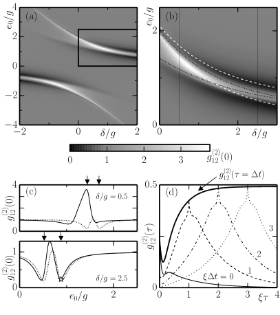
Figure 4: (a) Normalized cross correlation at zero time delay $g^{(2)}_{12}(0)$ as defined in Eq. (37) as a function of detuning $\delta$ and two-photon energy $e_{0}=2\nu_{0}-2\omega_{c}$ as defined in the previous figure caption. (b) Inset in (a) (see black box) together with the two photon energies depicted in Fig. 2(a) (dashed and dotted lines with the same notation as in Fig. 2(a)). (c) Cuts through (b) at constant detuning (indicated with vertical lines in (b)) for wave packets of width $\xi/\kappa=0.1$. The dotted lines correspond to the linear approximation, where correlation contributions due to the $T$-matrix elements in Eq. (26) are neglected. The arrows correspond to $2\Omega^{(1,2)}_{+}$. (d) Time-dependence of the normalized second-order cross correlation function for the parameter values indicated by the star in the lower panel of (c), i.e., for almost ideal HOM conditions, but for different time delay $\Delta t$ of the initial single-photon wave packets. The cross correlation function displays characteristic side peaks at time delay $\Delta t$, whose height, i.e. $g^{(2)}_{12}(\tau=\Delta t)$ converges at large time delays ($\Delta t\gg 1/\xi\gg 1/\kappa$), i.e. for completely distinguishable photon wave packets, towards $1/2$ (see text for explanation).

Figures 4(a) and (b) show that the HOM effect at $2\nu_{0}\approx 2\Omega^{(1,2)}_{\sigma}$ (dashed lines) manifests itself as a suppression of the cross correlations at zero time-delay with $g^{(2)}_{12}(0)\approx 0$ only in the dispersive regime ($|\delta|\gg g$) for upper polaritons at positive detuning ($\delta>0$) and lower polaritons at negative detuning ($\delta<0$), where nonlinear effects are weak and the JC nonlinearity acts as an almost ideal beam splitter. The different behavior at small and large detuning is analyzed in more detail in Figures 4(c) showing cuts through the inset in 4(b) (indicated by vertical lines): strong deviations from the linear result (dotted lines) are observed for small detuning (upper panel), but can be neglected for $|\delta|\gg g$ (lower panel). The zero-time delay cross correlation function $g^{(2)}_{12}(0)$ thus provides a useful signature for path entanglement only in the dispersive regime. Note that for an ideal HOM effect in the dispersive regime with $\gamma=0$ the wave-packet width should also tend to zero. The nonlinear effects at small detuning will be discussed in the next subsection further below.

The quantum interference process leading to the HOM effect relies on the indistinguishability of the two photons at zero time delay and equal energies. Thus, a time delay between the incoming photons leads to distinguishability and suppresses the HOM interference. Figure 4 (d) shows the cross correlation function with a time delay $\Delta t$ of the two photon wave packets in the dispersive regime for parameter settings corresponding to the star in the lower panel of Figs. 4(c) (HOM condition). We observe broad peaks centered at the time delay $\tau\approx\Delta t$, where the first photon has maximal overlap with the second. The overall width $\sim 1/\xi$ of the side peak is given by the width of the wave packet while the cusp like feature on top arises due to the coupling to the waveguides $\sim 1/\kappa$ and is suppressed in the limit $\xi/\kappa\rightarrow 0$. For large time delay and sharp wave packets such that $\Delta t\gg 1/\xi\gg 1/\kappa$, the cross correlation function is given by

$$G^{(2)}_{12}(\tau)\approx\frac{\xi}{8}\left(e^{-\xi|\tau-\Delta t|}+e^{-\xi|\tau+\Delta t|}\right)\,,$$ (39)

which yields the asymptotic value $g^{(2)}_{12}(\tau=\Delta t)\approx 1/2$ in agreement with Figure 4(d). The asymptotic value of $1/2$ originates from the fact, that only one of the two classical processes contributes to $G^{(2)}_{12}(\tau=\Delta t)$ while the normalisation in Eq. (38) is obtained by summing over both classical paths.

The appearance of a maximum in the cross correlation function at finite times thus serves as a measure for the distinguishability of the two photons due to an initial time delay and can be used to benchmark the two single photon sources attached to both transmission lines. These findings, valid in the dispersive regime, are consistent with recent experimental circuit QED results for a static, linear $50/50$ beam splitter in Refs. lang2013 ; woolley2013 .

V.2 Signatures of photon nonlinearities

In the previous subsection, we mostly discussed signatures of the HOM effect in the dispersive regime, where nonlinear effects can be neglected. We will now focus on a discussion of the resonant regime, where photon nonlinearities are strong.

When both photons are resonant with the one-polariton state ($2\nu_{0}=2\varepsilon_{1,\pm}$), dipole-induced transparency with reflection amplitude $r_{\nu=\varepsilon_{1,\pm}}=0$ (cf. Fig. 2 (b)) would lead to complete and independent transmission of the two particles in the absence of any correlations, i.e., if one neglects the contributions of the $T$-matrix in Eq. (35). However, when qubit and cavity are on resonance ($\delta\approx 0$), those contributions dominate and lead to photon blockade. In that case, a single photon already present in the cavity blocks the transmission of a second photon, which is thus reflected and preferentially drags the cavity-photon into the same waveguide leading to bunched correlations with $g_{11}^{(2)}(0)\gg 1$ (see Fig. 5(a)). Interestingly, when the total energy of both photons matches the two-polariton state energy ($2\nu_{0}=\varepsilon_{2,\pm}$), bunched as well as anti-bunched correlations can be observed, depending on the value of the detuning parameter .

Note, that this behaviour should be contrasted with the case, where both photons impinge on the qubit-cavity system from the same waveguide, i.e., for an incoming state $|\psi_{\rm in}\rangle\sim\iint d\nu_{1}d\nu_{2}f^{\rm\scriptscriptstyle(1)}_{\nu_{1}}f^{\rm\scriptscriptstyle(2)}_{\nu_{2}}a^{\dagger}_{1\nu_{1}}a^{\dagger}_{1\nu_{2}}|0\rangle$. This case is shown in Fig. 5(c), where photon blockade at $2\nu_{0}=2\varepsilon_{1,\pm}$ leads to bunching in reflection (right panel), but anti-bunching in transmission (left panel). In the latter case, bunching correlations are found for energies lying between the two anti-bunched regions. These findings are in agreement with previous theoretical shi:11 as well as experimental studies reinhard2012 .

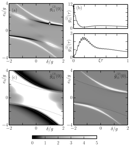
Figure 5: (a) Normalized auto-correlation function $g^{(2)}_{11}(0)$ at zero time delay as defined in Eq. (37) as a function of detuning $\delta$ and two-photon energy $e_{0}=2\nu_{0}-2\omega_{c}$ for two photons incoming from different waveguides ($\xi/\kappa=0.1$). (b) Time-dependence of the auto-correlation function $g^{(2)}_{11}(\tau)$ for the case of bunching (upper panel, indicated by star in (a)) and anti-bunching (lower panel, indicated by circle in (a)). (c) Normalized correlation function of transmitted (left) and reflected (right) photons $\tilde{g}^{(2)}_{22}(0)$ and $\tilde{g}^{(2)}_{11}(0)$ at zero time delay for two photons incoming from the same waveguide 1. Here, the dotted lines indicate the resonances at $2\varepsilon_{1,+}$ and $\varepsilon_{2,+}$, with the same notation as in Fig. 2(a). Note, that the correlation functions are cut-off at an arbitrarily chosen value $\tilde{g}^{(2)}_{ii}(0)<5$.

VI Conclusion

In this work, we have studied in detail the interplay of quantum interference leading to the HOM effect and effective photon-photon interactions in a waveguide QED system, where two single photon wave packets are incident on a Jaynes-Cummings nonlinearity from two separate waveguides. For this purpose, we have calculated the cross and auto-correlation functions of the two waveguides analytically based on a scattering matrix approach. A central result of our study is that the proposed setup can be used as an in-situ tunable HOM interferometer in the dispersive regime for already moderate detuning between the two-level system and the cavity and rather sharp wave packets of width $\xi$ smaller than the cavity decay width $\kappa$. In the opposite regime, where two-level system and cavity are on resonance, HOM interference is washed out and signatures of photon blockade due to effective photon-photon interactions induced by strong coupling of photons and two-level system, manifest as bunched correlations in the second-order auto-correlation function.

Appendix A Derivation of the scattering matrix

A.1 Even/odd modes

To calculate the one and two-photon scattering matrix in (9) and (10), it is convenient to first decompose the modes of waveguides $1$ and $2$ into even and odd modes shen:07 ; shi:09 by introducing

$$a^{(e,o)}_{\nu}=(a_{1\nu}\pm a_{2\nu})/\sqrt{2}$$ (40)

and rewriting the waveguide Hamiltonian as $H_{\rm w}=H_{\rm w}^{(e)}+H_{\rm w}^{(o)}$ with $H_{\rm w}^{(e,o)}=\int d\nu\,\nu\,a^{(e,o)\dagger}_{\nu}a^{(e,o)}_{\nu}$. With this transformation only the even modes couple to the cavity via

$$V=\sqrt{2}g_{\mathrm{w}}\int d\nu\,(b^{\dagger}a^{(e)}_{\nu}+ba^{(e)\dagger}_{\nu})\,,$$ (41)

and thus the Hamiltonian for the odd modes becomes trivial. The scattering matrix associated with the odd modes is given simply by the identity matrix. The Hamiltonian in the even modes,

$$H^{(e)}=H^{(e)}_{\rm w}+H_{\rm\scriptscriptstyle JC}+V,$$ (42)

then describes one chiral mode linearly coupled to the cavity. The scattering matrix for the even modes is nontrivial and can be calculated using the formalism in Ref. pletyukhov2012, (see next section).

Once we have calculated the one photon scattering matrices in the even subspace, i.e., $S^{(e)}_{\nu^{\prime}\nu}=\langle 0|a^{(e)}_{\nu^{\prime}}Sa^{(e)\dagger}_{\nu}|0\rangle$, we transform back to physical space via the relations

$$S^{11}_{\nu^{\prime}\nu} = S^{22}_{\nu^{\prime}\nu}=\frac{1}{2}(S^{(e)}_{\nu^{\prime}\nu}+\delta_{\nu^{\prime}\nu})$$ (43)

$$S^{12}_{\nu^{\prime}\nu} = S^{21}_{\nu^{\prime}\nu}=\frac{1}{2}(S^{(e)}_{\nu^{\prime}\nu}-\delta_{\nu^{\prime}\nu})\,,$$ (44)

where the delta function on the right hand side stems from the trivial contribution of the odd modes. From the two-photon scattering matrix in the even space $S^{(e)}_{\nu^{\prime}_{1}\nu^{\prime}_{2}\nu_{1}\nu_{2}}=\langle 0|a^{(e)}_{\nu^{\prime}_{2}}a^{(e)}_{\nu^{\prime}_{1}}Sa^{(e)\dagger}_{\nu_{1}}a^{(e)\dagger}_{\nu_{2}}|0\rangle=S^{(e)}_{\nu^{\prime}_{1}\nu_{1}}S^{(e)}_{\nu^{\prime}_{2}\nu_{2}}+S^{(e)}_{\nu^{\prime}_{1}\nu_{2}}S^{(e)}_{\nu^{\prime}_{2}\nu_{1}}+i\mathcal{T}^{(2e)}_{\nu^{\prime}_{1}\nu^{\prime}_{2},\nu_{1}\nu_{2}}$ we obtain the two-photon scattering matrix in Eq. (10) from the results above together with the simple relation

$$\mathcal{T}^{(2)}_{\nu^{\prime}_{1}\nu^{\prime}_{2},\nu_{1}\nu_{2}}=\mathcal{T}^{(2e)}_{\nu^{\prime}_{1}\nu^{\prime}_{2},\nu_{1}\nu_{2}}/4\,.$$ (45)

A.2 $T$-matrix

To calculate the single- and two-photon scattering matrix of the even modes we make use of the formalism introduced in Ref. pletyukhov2012, . The scattering matrix is conveniently expressed through the $T$-matrix which contains the non-trivial part of the scattering, i.e.,

$$S=1-2\pi i\,\delta(E_{\rm in}-E_{\rm out})T(E_{\rm in})$$ (46)

with the energies $E_{\rm in}$ and $E_{\rm out}$ of the incoming resp. outgoing state. The $T$-matrix can be expressed through the full Green’s function $\hat{G}(\omega)=(\omega-H+i0^{+})^{-1}$ with $H^{(e)}$ defined in Eq. (42) as

$$T(\omega)=V+V\hat{G}(\omega)V\,.$$ (47)

The series representation of the full Green’s function $\hat{G}(\omega)=\sum_{n=0}^{\infty}G_{0}(\omega)\left[VG_{0}(\omega)\right]^{n}$ in terms of the free Green’s function $G_{0}(\omega)=(\omega-H_{0}+i0^{+})^{-1}$ and the interaction $V$ given in Eq. (41) yields the corresponding series representation of the $T$-matrix. For photon number conserving scattering processes we obtain $T(\omega)=V\sum_{n=1}^{\infty}\left[G_{0}(\omega)V\right]^{n}$. The main result of Ref. pletyukhov2012, is to show that the $T$-matrix for an incoming $N$-photon state can be expressed as

$$T^{(N)}(\omega)=\vdots\,G_{0}^{-1}\tilde{G}\left(V\tilde{G}\right)^{2N}G_{0}^{-1}\,\vdots\,,$$ (48)

with the dressed Green’s function

$$\tilde{G}(\omega)=(\omega-H_{0}-\Sigma)^{-1}\,,$$ (49)

where the operator $\Sigma$ (of the form of a self-energy) accounts for the coupling of the atomic system to the waveguide and for the linear coupling in Eq. (41) attains the remarkably simple form

$$\Sigma=-2i\pi g_{\mathrm{w}}^{2}b^{\dagger}b\,.$$ (50)

The operation $\vdots(\,\,)\vdots$ is a version of the normal ordering, which removes contractions in pairs of $V$’s, but does not account for contractions between $V$ and $H_{0}$. The latter can be effectively accounted for by shifts in $\omega$-arguments of the dressed Green’s functions $\tilde{G}$ occurring in the expansion (48).

A.3 Scattering matrix for even modes

We are now in the position to calculate, e.g., the one photon scattering matrix elements

$$S^{(e)}_{\nu^{\prime}\nu} = \langle 0|a^{(e)}_{\nu^{\prime}}Sa^{(e)\dagger}_{\nu}|0\rangle=\delta(\nu^{\prime}-\nu)$$

$$-2\pi i\delta(\nu^{\prime}-\nu)\langle 0|a^{(e)}_{\nu^{\prime}}T^{(1)}(\nu)a^{(e)\dagger}_{\nu}|0\rangle$$

from the result in (48), i.e.,

$$T^{(1)}(\omega)=\vdots\,G_{0}^{-1}(\omega)\tilde{G}(\omega)V\tilde{G}(\omega)V\tilde{G}(\omega)G_{0}^{-1}(\omega)\,\vdots\,.$$ (52)

Here, the combination $\tilde{G}(E_{\rm in})G_{0}^{-1}(E_{\rm in})$ at the end of the operator chain on the r.h.s of Eq. (52) acts as a projector on the dark states (non-broadened states). This can be seen from the expression $\tilde{G}(E_{\rm in})G_{0}^{-1}(E_{\rm in})|\psi_{\rm in}\rangle$, which is zero for any incoming eigenstate of $H_{0}$ since $G_{0}^{-1}(E_{\rm in})=(E_{\rm in}-H_{0})$ except when $\tilde{G}(E_{\rm in})=G_{0}(E_{\rm in})$, i.e., for the non-broadened states with $\Sigma|\psi_{\rm in}\rangle=0$. In the case of the JC nonlinearity, the only non-broadened state is the ground state of the combined cavity-qubit system $|\psi_{0}\rangle=|0,\downarrow\rangle$, such that we can replace $\tilde{G}(E_{\rm in})G_{0}^{-1}(E_{\rm in})$ by the projector $P_{0}=|\psi_{0}\rangle\langle\psi_{0}|$. The same is true for $G_{0}^{-1}(E_{\rm in})\tilde{G}(E_{\rm in})$ on the left of the expression (as $E_{\rm in}=E_{\rm out}$). By expressing the dressed Greens function in (49) through the projector $\tilde{P}_{n\sigma}=|\tilde{\psi}_{n\sigma}\rangle\langle\tilde{\psi}_{n\sigma}|$ on the Jaynes-Cummings resonances $|\tilde{\psi}_{n\sigma}\rangle$ (given by the expressions for $|\psi_{n\sigma}\rangle$ in (5) with the angle $\theta_{n}$ replaced by $\tilde{\theta}_{n}$ with $\omega_{c}\rightarrow\tilde{\omega}_{c}=\omega_{c}-i\kappa$) as $\tilde{G}(\omega)=\sum_{n\alpha}\tilde{P}_{n\alpha}(\omega-H_{\rm w}-\tilde{\varepsilon}_{n\alpha})^{-1}$ and calculating the corresponding matrix elements in (52), one arrives at the final result $S_{\nu^{\prime}\nu}^{(e)}=s_{\nu}^{(e)}\delta(\nu^{\prime}-\nu)$ with

$$s_{\nu}^{(e)}=\frac{(\nu-\tilde{\varepsilon}_{1+}^{\ast})(\nu-\tilde{\varepsilon}_{1-}^{\ast})}{(\nu-\tilde{\varepsilon}_{1+})(\nu-\tilde{\varepsilon}_{1-})}.$$ (53)

A similar calculation for the two-photon $T$-matrix

$$T^{(2)}(\omega)=\vdots\,P_{0}V\tilde{G}(\omega)V\tilde{G}(\omega)V\tilde{G}(\omega)VP_{0}\,\vdots$$ (54)

yields after some lengthy algebra the result stated in Eq. (III).

Appendix B Strongly dispersive regime: Limit of Kerr nonlinearity and TLS scattering matrix

We show here, that in the dispersive limit $\delta\gg g$ the JC scattering matrix given by Eqs. (13), (14), and (III) can be simplified to the scattering matrix of the Kerr nonlinearity for incoming photon energies $\nu_{0i}\approx\omega_{c}$ and to the scattering matrix of a TLS for energies $\nu_{0i}\approx\omega_{q}$. [The limit $-\delta\gg g$ can be treated analogously.]

Let us start with the Kerr regime: We approximate the energies (7) as $\varepsilon_{n+}=\omega_{c}+ng^{2}/\delta-n^{2}g^{4}/\delta^{3}$, such that the two lowest levels effectively form a Kerr nonlinearity with $\varepsilon_{1+}=\bar{\omega}_{c}$ and $\varepsilon_{2+}=2\bar{\omega}_{c}+U$ with $\bar{\omega}_{c}\approx\omega_{c}+g^{2}/\delta-g^{4}/\delta^{3}$ and $U\approx-2g^{4}/\delta^{3}$. The energies of the off-resonant states $|\psi_{n-}\rangle$ are approximated as $\varepsilon_{n-}\approx n\omega_{c}-\delta$. To approximate the single-photon scattering matrix coefficients $t_{\nu}$ and $r_{\nu}$ given by Eqs. (13) and (14), it is useful to note that they can be written as $r_{\nu}=(s_{\nu}^{(e)}+1)/2$ and $t_{\nu}=(s_{\nu}^{(e)}-1)/2$. As $\tilde{\varepsilon}_{1-}$ is off-resonant, we approximate $\nu-\tilde{\varepsilon}_{1-}\approx\varepsilon_{1+}-\tilde{\varepsilon}_{1-}\approx\delta$ which leads to $s_{\nu}^{(e)}=(\nu-\bar{\omega}_{c}-i\kappa)/(\nu-\bar{\omega}_{c}+i\kappa)$ in agreement with Ref. liao:10, and to $r_{\nu}=(\nu-\bar{\omega}_{c})/(\nu-\bar{\omega}_{c}+i\kappa)$ and $t_{\nu}=-i\kappa/(\nu-\bar{\omega}_{c}+i\kappa)$. In the same way, we approximate the $T$-matrix given by Eq. (III): Only the single-photon resonances at energy $\varepsilon_{1+}$, the two photon resonances at energies $\varepsilon_{2+}$, as well as the energy dependence in $\nu_{1}+\nu_{2}-2\varepsilon_{1+}$ are relevant. In all the other factors which do not contain $\varepsilon_{n+}$ we approximate $\nu_{i}\approx\varepsilon_{1+}$ and obtain to leading order in $g/\delta$

$$\mathcal{T}^{(2)}_{\nu^{\prime}_{1}\nu^{\prime}_{2},\nu_{1}\nu_{2}} \approx-\frac{\kappa^{2}U}{\pi}\frac{\nu_{1}+\nu_{2}-2\bar{\omega}_{c}+2i\kappa}{\nu_{1}+\nu_{2}-2\bar{\omega}_{c}-U+2i\kappa}$$ (55)

$$\quad\times\frac{\delta_{\nu^{\prime}_{1}+\nu^{\prime}_{2},\nu_{1}+\nu_{2}}}{\prod_{i=1,2}(\nu^{\prime}_{i}-\bar{\omega}_{c}+i\kappa)(\nu_{i}-\bar{\omega}_{c}+i\kappa)},$$

with $\bar{\omega}_{c}$ and $U$ as introduced above.

For incoming photon energies $\nu_{0i}$ close to $\varepsilon_{1-}$, we proceed similarly. In this regime, only the resonance at $\tilde{\varepsilon}_{1-}$ is relevant which we approximate to leading order in $g/\delta$ by $\tilde{\varepsilon}_{1-}=\bar{\omega}_{q}-i\bar{\kappa}$ with $\bar{\omega}_{q}=\omega_{q}-g^{2}/\delta$ and $\bar{\kappa}=\kappa g^{2}/\delta^{2}$. All the other factors which do not contain $\tilde{\varepsilon}_{1-}$ are off-resonant and approximated by $\tilde{\varepsilon}_{n+}\approx\varepsilon_{n+}\approx n\omega_{c}$ and $\tilde{\varepsilon}_{n-}\approx\varepsilon_{n-}\approx n\omega_{c}-\delta$ for $n>1$. Approximating $\nu-\tilde{\varepsilon}_{1+}\approx-\delta$ in Eq. (53), we obtain $s_{\nu}^{(e)}=(\nu-\bar{\omega}_{q}-i\bar{\kappa})/(\nu-\bar{\omega}_{q}+i\bar{\kappa})$, in agreement with Ref. shen:07, . Similarly as above, we approximate $\nu_{i}$ in all terms by $\omega_{q}$, except for the single photon resonance at $\tilde{\varepsilon}_{1-}$ and in the factor $\nu_{1}+\nu_{2}-2\tilde{\varepsilon}_{1-}$, and obtain to leading order in $g/\delta$

$$\mathcal{T}^{(2)}_{\nu^{\prime}_{1}\nu^{\prime}_{2},\nu_{1}\nu_{2}} \approx\frac{\bar{\kappa}^{2}}{\pi}\frac{\delta_{\nu^{\prime}_{1}+\nu^{\prime}_{2},\nu_{1}+\nu_{2}}(\nu_{1}+\nu_{2}-2\bar{\omega}_{q}+2i\bar{\kappa})}{\prod_{i=1,2}(\nu^{\prime}_{i}-\bar{\omega}_{q}+i\bar{\kappa})(\nu_{i}-\bar{\omega}_{q}+i\bar{\kappa})},$$ (56)

in agreement with the result for the TLS in Ref. shen:07, .

References

• (1) C.K. Hong, Z.Y. Ou, and L. Mandel, Phys. Rev. Lett. 59, 2044 (1987).
• (2) H.J. Kimble, Nature 453, 1023 (2008).
• (3) E. Knill, R. Laflamme, and G.J. Milburn, Nature 409, 46 (2001).
• (4) C. Santori, D. Fattal, J. Vučković. G.S. Solomon, and Y. Yamamoto, Nature 419, 594 (2002).
• (5) H. de Riedmatten, I. Marcikic, W. Tittel, H. Zbinden, and N. Gisin, Phys. Rev. A 67, 022301 (2003).
• (6) T. Legero, T. Wilk, M. Hennrich, G. Rempe, and A. Kuhn, Phys. Rev. Lett. 93, 070503 (2004).
• (7) J. Beugnon, M.P.A. Jones, J. Dingjan, B. Darquié, G. Messin, A. Browaeys, and P. Grangier, Nature 440, 779 (2006).
• (8) P. Maunz, D.L. Moehring, S. Olmschenk, K.C. Younge, D.N. Matsukevich, and C. Monroe, Nat. Phys. 3, 538 (2007).
• (9) A. Blais, R.-S. Huang, A. Wallraff, S.M. Girvin and R.J. Schoelkopf, Phys. Rev. A 69, 062320 (2004).
• (10) A. Wallraff, D.I. Schuster, A. Blais, L. Frunzio, R.-S. Huang, J. Majer, S. Kumar, S.M. Girvin, and R.J. Schoelkopf, Nature 431, 162 (2004).
• (11) P. Longo, J.H. Cole, and K. Busch, Optics Express 20, 12326 (2011).
• (12) M. Laakso and M. Pletyukhov, Phys. Rev. Lett. 113, 183601 (2014).
• (13) C. Lang, C. Eichler, L. Steffen, J.M. Fink, M.J. Woolley, A. Blais, and A. Wallraff, Nature Physics 9, 345 (2013).
• (14) M.J. Woolley, C. Lang, C. Eichler, A. Wallraff, and A. Blais, New J. Phys. 15, 105025 (2013).
• (15) T. Shi, S. Fan, and C.P. Sun, Phys. Rev. A 84, 063803 (2011).
• (16) A.A. Houck, D.I. Schuster, J.M. Gambetta, J.A. Schreier, B.R. Johnson, J.M. Chow, L. Frunzio, J. Majer, M.H. Devoret, S.M. Girvin, and R.J. Schoelkopf, Nature 449, 328 (2007).
• (17) C. Lang, D. Bozyigit, C. Eichler, L. Steffen, J.M. Fink, A.A. Abdumalikov, Jr., M. Baur, S. Filipp, M.P. da Silva, A. Blais, and A. Wallraff, Phys. Rev. Lett. 106, 243601 (2011).
• (18) M. Pletyukhov and V. Gritsev, New J. Phys. 14, 095028 (2012).
• (19) S. Schmidt and J. Koch, Annalen der Physik 525, 395 (2013).
• (20) E. Waks and J. Vuckovic, Phys. Rev. Lett. 96, 153601 (2006).
• (21) J.T. Shen and S. Fan, Phys. Rev. A 79, 023837 (2009).
• (22) J.T. Shen and S. Fan, Phys. Rev. A 76, 062709 (2007).
• (23) T. Shi and C.P. Sun, Phys. Rev. B 79, 205111 (2009).
• (24) J.-Q. Liao and C.K. Law, Phys. Rev. A 82, 053836 (2010).
• (25) A. Reinhard, T. Volz, M. Winger, A. Badolato, K.J. Hennessy, E. Hu, and A. Imamoglu, Nature Photonics 6, 93–96 (2012).