$X(3872)$ electromagnetic decay in a coupled-channel model

Abstract

A multichannel Schrödinger equation with both quark-antiquark and meson-meson components, using a harmonic-oscillator potential for $q\bar{q}$ confinement and a delta-shell string-breaking potential for decay, is applied to the axial-vecor $X(3872)$ and lowest vector charmonia. The model parameters are fitted to the experimental values of the masses of the $X(3872)$, $J/\psi$ and $\psi(2S)$. The wave functions of these states are computed and then used to calculate the electromagnetic decay widths of the $X(3872)$ into $J/\psi\gamma$ and $\psi(2S)\gamma$.

12.39.Pn,12.40.Yx,13.20.Gd,13.40.Hq

1 Introduction

The $X(3872)$ was discovered in 2003 by the Belle Collaboration [1], and later confirmed in CDF [2] and D0 [3] experiments. Its PDG[4] mass and width are now $M_{X}=3871.69\pm 0.17\,\mbox{MeV}$ and $\Gamma_{X}<1.2\,\mbox{MeV}$, respectively. According to experiment it has quantum numbers $J^{PC}=1^{++}$[5] and $I^{G}=0^{+}$ [6, 7]. The $X(3872)$ seems to be difficult to describe as a simple $c\bar{c}$ state.

Its main decays are into $\rho^{0}J/\psi$, $\omega J/\psi$ and $DD\pi$, with the latter final state resulting mainly from an intermediate $DD^{*}$ channel. The first two channels are OZI forbidden and the decay into $\rho^{0}J/\psi$ also violates isospin conservation. Both are therefore highly suppressed. As the mass is below the $DD^{*}$ thresholds ($E_{D^{0}D^{0*}}=3871.84$ MeV and $E_{D^{\pm}D^{\mp*}}=3879.90$ MeV), which are the lowest OZI-allowed decay channels, the $X(3872)$ can be seen as a quasi-bound state.

Here we will study the $X(3872)$ as a unitarized mesonic state, that is, one with both quark-antiquark and meson-meson (MM) components. A previous configuration-space calculation [8] with $c\bar{c}$ and $D^{0}D^{0*}$components predicted a state with approximately $7.5\%$ $c\bar{c}$. We now generalize that calculation to include other possible channels.

Electromagnetic (EM) decays of the $X(3872)$ were observed by Belle [9], Babar [10] and LHCb [11]. Babar and LHCb observed decays into $J/\psi\gamma$ and $\psi(2S)\gamma$, and found the ratio of partial decay widths

$$\mathcal{R}_{\psi}=\frac{\Gamma(\psi(2S)\gamma)}{\Gamma(J/\psi\gamma)}$$

to be of the order of 2.5–3.5, whereas Belle did not observe the decay into $\psi(2S)\gamma$ at all and set an upper limit on the value of $\mathcal{R}_{\psi}$ (see Table 1).

Collaboration	$\mathcal{R}_{\psi}$
Belle [9]	$<2.1$
BaBar [10]	$3.4\pm 1.4$
LHCb [11]	$2.46\pm 0.64\pm 0.29$

Table 1: Measured values of the EM rate ratio $\mathcal{R}_{\psi}$.

2 Method

We first derive the wave functions of $J/\psi$, $\psi(2S)$ and $X(3872)$, considering all $c\bar{c}$, $DD$ (only for vector charmonia), $DD^{*}$ and $D^{*}D^{*}$ channels, where $D^{(*)}$ is shorthand for $D^{(*)0}$, $D^{(*)\pm}$, or $D_{s}^{(*)\pm}$. With these, the EM transition matrix elements and resulting decay widths will be calculated.

In the present model, a unitarized meson is not just a $q\bar{q}$ state but it also has MM components:

$$|\psi\rangle=\sum_{c}|\psi_{q\bar{q}}^{c}\rangle+\sum_{j}|\psi_{MM}^{j}\rangle\;.$$ (2.1)

In the quark-antiquark sector we have confinement realized through a harmonic-oscillator (HO) potential with universal (i.e., mass-independent) frequency:

$$V_{Q\bar{Q}}(r)=\frac{1}{2}\mu_{c}\omega^{2}r^{2}\;.$$ (2.2)

As for the MM sector, we assume no direct interactions and only a string-breaking potential that links the $q\bar{q}$ and MM channels to one another:

$$V_{cj}=\frac{\lambda g_{cj}}{2\mu_{c}}\delta(r-a)\;.$$ (2.3)

We take the parameters $m_{c}=1.562\,\mbox{GeV}$ and $\omega=0.190\,\mbox{GeV}$ unchanged with respect to all our previous work. In the $1^{--}$ and $1^{++}$ cases, somewhat different values of the overall coupling $\lambda$ will be applied, viz. $\lambda_{\psi}$ and $\lambda_{X}$, respectively, to be determined from the physical charmonium masses. Furthermore, the $J/\psi$ and $\psi(2S)$ masses will also be used to fix the value of the string-breaking distance $a$, which we will take the same for the $X(3872)$. Finally, the $g_{cj}$ are ${}^{3\!}P_{0}$ coupling coefficients.

Next we solve the coupled-channel Schrödinger equation

$$\left[\begin{array}[]{cc}\hat{h}_{q\bar{q}}^{c}&V_{cj}\\ V_{jc}^{\dagger}&\hat{h}_{MM}^{j}\end{array}\right]\left[\begin{array}[]{c}u_{c}\\ v_{j}\end{array}\right]=E\left[\begin{array}[]{c}u_{c}\\ v_{j}\end{array}\right]\;,$$ (2.4)

with

$$\hat{h}_{q\bar{q}}^{c} = m_{q}^{c}+m_{\bar{q}}^{c}+\frac{\hbar^{2}}{2\mu_{c}}\big{(}-\frac{d^{2}}{dr^{2}}+\frac{l_{c}(l_{c}+1)}{r^{2}}\big{)}+\frac{1}{2}\mu_{c}\omega^{2}r^{2}\;,$$

$$\hat{h}_{MM}^{j} = M_{1}^{j}+M_{2}^{j}+\frac{\hbar^{2}}{2\mu_{j}}\big{(}-\frac{d^{2}}{dr^{2}}+\frac{L_{j}(L_{j}+1)}{r^{2}}\big{)}\;.$$

The solutions are known for $r\neq a$ and appropriate boundary conditions:

$$u_{c}(r)=\left\{\begin{array}[]{r}\!\!\!a_{c}M(-\nu_{c},l_{c}+\frac{3}{2},\mu_{c}\omega r^{2})e^{-\frac{1}{2}\mu_{c}\omega r^{2}}r^{1+l_{c}}\;,\;\;\;r<a\;,\\ \!\!\!b_{c}U(-\nu_{c},l_{c}+\frac{3}{2},\mu_{c}\omega r^{2})e^{-\frac{1}{2}\mu_{c}\omega r^{2}}r^{1+l_{c}}\;,\;\;\;r>a\;,\end{array}\right.$$ (2.5)

and

$$v_{j}(r)=\left\{\begin{array}[]{r}\!\!\!A_{j}i_{L_{j}}(q_{j}r)\,r\;,\;\;\;r<a\;,\\ \!\!\!B_{j}k_{L_{j}}(q_{j}r)\,r\;,\;\;\;r>a\;.\end{array}\right.$$ (2.6)

Using now continuity of the wave function and discontinuity of its derivative, we can solve the equations for $a_{c}$, $b_{c}$, $A_{j}$ and $B_{j}$. The value of the energy $E$ (for fixed $\lambda$) or coupling $\lambda$ (for fixed $E$) is then given by the equation ($\alpha_{c}\equiv a_{c}M_{c}$)

$$\Big{(}\frac{U_{c}^{\prime}}{U_{c}}-\frac{M_{c}^{\prime}}{M_{c}}\Big{)}\alpha_{c} =\lambda^{2}\sum_{jd}\frac{\mu_{j}g_{cj}}{2\mu_{c}\omega q_{j}a^{3}}\Big{(}\frac{k{}_{j}^{\prime}}{k_{j}}-\frac{i_{j}^{\prime}}{i_{j}}\Big{)}^{-1}\>\frac{e^{\frac{1}{2}(\mu_{c}-\mu_{d})\omega a^{2}}g_{dj}}{\mu_{d}}\,\alpha_{d}\;.$$ (2.7)

For more details, see [12].

3 Wave functions

Using the method outlined in Sec. 2, and fitting $\lambda_{\psi}$ as well as $a$ to the experimental $J/\psi$ and $\psi(2S)$ masses, we find $\lambda_{\psi}=2.53$ and $a=1.95$ GeV^-1. The resulting wave-function components are plotted in Fig. 3.1. Next

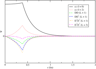
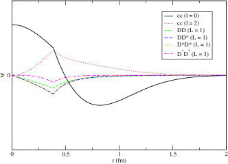
Figure 3.1: Wave-function components of the $J/\psi$ and $\psi(2S)$

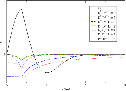
Figure 3.2: Wave-function components of the $X(3872)$

we adjust $\lambda_{X}$ to the $X(3872)$ mass while keeping $a$ the same, which yields the wave-function components shown in Fig. 3.2. The three wave-function compositions are given in Table 2. We see that

	$c\bar{c}$	$DD$	$D^{0}D^{*0}$	$D^{\pm}D^{*\mp}$	$D^{*}D^{*}$
$J/\psi$	83.6%	2.1%	6.0%		8.3%
$\psi(2S)$	94.5%	1.3%	2.1%		2.1%
$X(3872)$	26.8%	-	65.0%	7.0%	1.2%

Table 2: Compositions of the three charmonia ($D^{(*)}$: shorthand, see text.)

the $J/\psi$ and $\psi(2S)$ are mostly $c\bar{c}$ states, whereas the $X(3872)$ has a dominant $D^{0}D^{*0}$ component. Still, its $c\bar{c}$ probability of 26.8% is a huge increase as compared to the 7.5% in [8].

4 Electromagnetic decay

To compute the EM decay widths we use the Fermi golden rule

$$\Gamma_{i\rightarrow f}=\frac{2\pi}{\hbar}|\langle\Psi_{f}|\hat{H}_{int}|\Psi_{i}\rangle|\rho_{f}\;,$$ (4.1)

with density of states $\rho_{f}=\frac{1}{2\pi\hbar c}$ [13]. To evaluate the matrix elements in 4.1, we note that the initial and final states are given by $|\Psi_{i}\rangle=|\psi_{nJM}\rangle\otimes|0\rangle$ and $|\Psi_{f}\rangle=|\psi_{n^{\prime}J^{\prime}M^{\prime}}\rangle\otimes|\gamma_{\lambda klm}\rangle$, where $l$ and $m$ are the angular-momentum quantum numbers, and $\lambda$ the polarization.

Expanding the wave function, we get a matrix element

$$\langle\Psi_{f}|\hat{H}_{int}|\Psi_{i}\rangle=\sum_{cc^{\prime}}\langle\psi_{q\bar{q}}^{c}|\hat{h}_{int}^{cc^{\prime}}|\psi_{q\bar{q}}^{c^{\prime}}\rangle+\sum_{jj^{\prime}}\langle\psi_{MM}^{j}|\hat{h}_{int}^{jj^{\prime}}|\psi_{MM}^{j^{\prime}}\rangle\;,$$ (4.2)

as we only consider transitions of the types $(Q\bar{Q})^{*}\rightarrow Q\bar{Q}+\gamma$ and $(M_{1}M_{2})^{*}\rightarrow M_{1}M_{2}+\gamma$, neglecting those like $M_{1}^{*}M_{2}^{*}\rightarrow M_{1}M_{2}+\gamma$.

The interaction Hamiltonian $\hat{h}_{int}$ is obtained from minimal coupling, accounting for a possible anomalous magnetic moment. In the radiation gauge $\nabla.\mathbf{A}=0$ and $A^{0}=0$, and neglecting the $\mathbf{A}^{2}$ term, we have

$$\hat{h}_{int}=\sum_{i}\frac{iQ_{i}}{m_{i}c}\,\mathbf{A}(\mathbf{x}_{i})\cdot\nabla_{i}-\mu_{i}\mathbf{S}_{i}\cdot\mathbf{B}(\mathbf{x}_{i})\;.$$ (4.3)

The EM vector potential is expanded as

$$\mathbf{A}(\mathbf{r},t)=\sqrt{4\pi}\hbar c\sum_{\lambda lm}\int\frac{dk}{2\pi}\frac{1}{\sqrt{2\omega_{k}}}\big{[}\mathbf{f}_{klm}^{(\lambda)}(\mathbf{r})e^{-i\omega_{k}t}a_{\lambda lm}(k)+h.\,c.\big{]}\;,$$

with $a_{\lambda lm}$ being photon-annihilation operators. Components with $\lambda=e$ correspond to electric multipole radiation and the ones with $\lambda=m$ to magnetic multipole radiation. For the same $l$, they have opposite parity.

The $X(3872)$ ($1^{++}$ state) can only decay decay into $J/\psi$ and $\psi(2S)$ ($1^{--}$ states) by emitting electric-dipole ($l=1$) or magnetic-quadrupole ($l=2$) photons.

The computation of the matrix elements is carried out as in [13]. The resulting EM decay widths are presented in Table 3.

	Complete	$c\bar{c}$	MM	Quenched
$\Gamma_{e}(X\rightarrow J/\psi\gamma)$	24.2	14.9	1.11	0.48
$\Gamma_{m}(X\rightarrow J\psi\gamma)$	0.44	0.34	0.01	0.14
$\Gamma_{e}(X\rightarrow\psi^{\prime}\gamma)$	28.8	28.0	0.01	158
$\Gamma_{m}(X\rightarrow\psi^{\prime}\gamma)$	0.07	0.07	0.00	0.26

Table 3: Computed EM decay widths in keV. The second and third columns show the hypothetical widths from the $c\bar{c}$ and $MM$ components only. The last column gives the predictions of an HO quenched quark model, with the same $m_{c}$ and $\omega$ as in the unquenched case. Note that these numbers are slighty different from those presented at the workshop, after correction of minor numerical errors.

We obtain an EM rate ratio $\mathcal{R}_{\psi}=1.17$.

5 Conclusions

We have generalized a previous configuration-space calculation [8] of the $X(3872)$ by including more MM channels. Thus we obtained an increase of the total $c\bar{c}$ probability from $7.5\%$ to $26.8\%$. This seemingly paradoxical result has a simple explanation: the inclusion of more MM channels leads to a reduction of the $D^{0}D^{*0}$ component, which — due to its long tail — was responsible for an MM probability exceeding 90% [8]. Table 3 shows that unquenching very strongly affects the EM widths. Our prediction of the ratio $\mathcal{R}_{\psi}=1.17$ is consistent with the result of Belle, but does not fully agree with BaBar and LHCb. However, there is an enormous improvement when compared to a quenched HO calculation. For a more detailed discussion, see [12].

M. Cardoso was supported by FCT, contract SFRH/BPD/73140/2010.

References

• [1] S.-K.Β Choi etΒ al. [Belle Collaboration], Phys.Β Rev.Β Lett. 91, 262001 (2003).
• [2] D.Β Acosta etΒ al. [CDF Collaboration], Phys.Β Rev.Β Lett. 93, 072001 (2004).
• [3] V.Β M.Β Abazov etΒ al. [D0 Collaboration], Phys.Β Rev.Β Lett. 93, 162002 (2004).
• [4] K.Β A.Β Olive etΒ al. [Particle Data Group Collaboration], Chin.Β Phys. C38, 090001 (2014).
• [5] R.Β Aaij etΒ al. [LHCb Collaboration], Phys.Β Rev.Β Lett. 110, 222001 (2013).
• [6] B.Β Aubert etΒ al. [BaBar Collaboration], Phys.Β Rev. D71, 031501 (2005).
• [7] S.-K. Choi etΒ al. [Belle Collaboration], Phys.Β Rev. D84, 052004 (2011).
• [8] S.Β Coito, G.Β Rupp, E.Β van Beveren, Eur.Β Phys.Β J. C73, 2351 (2013).
• [9] V.Β Bhardwaj etΒ al. [Belle Collaboration], Phys.Β Rev.Β Lett. 107, 091803 (2011).
• [10] B.Β Aubert etΒ al. [BaBar Collaboration], Phys.Β Rev.Β Lett. 102, 132001 (2009).
• [11] R.Β Aaij etΒ al. [LHCb Collaboration], Nucl.Β Phys. B886, 665 (2014).
• [12] M.Β Cardoso, G.Β Rupp, E.Β van Beveren, arXiv:1411.1654v2 [hep-ph], accepted for publication in Eur.Β Phys.Β J.Β C.
• [13] A.Β G.Β M.Β Verschuren, C.Β Dullemond, E.Β van Beveren, Phys.Β Rev. D44, 2803 (1991).