Theoretical guarantees for approximate sampling from
smooth and log-concave densities

Abstract

Sampling from various kinds of distributions is an issue of paramount importance in statistics since it is often the key ingredient for constructing estimators, test procedures or confidence intervals. In many situations, the exact sampling from a given distribution is impossible or computationally expensive and, therefore, one needs to resort to approximate sampling strategies. However, there is no well-developed theory providing meaningful nonasymptotic guarantees for the approximate sampling procedures, especially in the high-dimensional problems. This paper makes some progress in this direction by considering the problem of sampling from a distribution having a smooth and log-concave density defined on $\mathbb{R}^{p}$, for some integer $p>0$. We establish nonasymptotic bounds for the error of approximating the target distribution by the one obtained by the Langevin Monte Carlo method and its variants. We illustrate the effectiveness of the established guarantees with various experiments. Underlying our analysis are insights from the theory of continuous-time diffusion processes, which may be of interest beyond the framework of log-concave densities considered in the present work.

1 Introduction

Let $p$ be a positive integer and $f:\mathbb{R}^{p}\to\mathbb{R}$ be a measurable function such that the integral $\int_{\mathbb{R}^{p}}\exp\{-f(\boldsymbol{\theta})\}\,d\boldsymbol{\theta}$ is finite. If we think of $f$ as the negative log-likelihood or the negative log-posterior of a statistical model, then the maximum likelihood and the Bayesian estimators, which are perhaps the most popular in statistics, are respectively defined as

$$\boldsymbol{\theta}^{{\rm ML}}\in\operatorname*{arg\,min}_{\boldsymbol{\theta}\in\mathbb{R}^{p}}f(\boldsymbol{\theta});\qquad\boldsymbol{\theta}^{{\rm B}}=\frac{1}{\int_{\mathbb{R}^{p}}e^{-f(\boldsymbol{u})}\,d\boldsymbol{u}}\int_{\mathbb{R}^{p}}\boldsymbol{\theta}e^{-f(\boldsymbol{\theta})}\,d\boldsymbol{\theta}.$$

These estimators are rarely available in closed-form. Therefore, optimisation techniques are used for computing the maximum-likelihood estimator while the computation of the Bayes estimator often requires sampling from a density proportional to $e^{-f(\boldsymbol{\theta})}$. In most situations, the exact computation of these two estimators is impossible and one has to resort to approximations provided by iterative algorithms. There is a vast variety of such algorithms for solving both tasks, see for example (Boyd and Vandenberghe, 2004) for optimisation and (Atchadé et al., 2011) for approximate sampling. However, a striking fact is that the convergence properties of optimisation algorithms are much better understood than those of the approximate sampling algorithms. The goal of the present work is to partially fill this gap by establishing easy-to-apply theoretical guarantees for some approximate sampling algorithms.

To be more precise, let us consider the case of a strongly convex function $f$ having a Lipschitz continuous gradient. That is, there exist two positive constants $m$ and $M$ such that

$$\begin{cases}f(\boldsymbol{\theta})-f(\bar{\boldsymbol{\theta}})-\nabla f(\bar{\boldsymbol{\theta}})^{\top}(\boldsymbol{\theta}-\bar{\boldsymbol{\theta}})\geq\frac{m}{2}\|\boldsymbol{\theta}-\bar{\boldsymbol{\theta}}\|_{2}^{2},\\ \|\nabla f(\boldsymbol{\theta})-\nabla f(\bar{\boldsymbol{\theta}})\|_{2}\leq M\|\boldsymbol{\theta}-\bar{\boldsymbol{\theta}}\|_{2},\end{cases}\qquad\forall\boldsymbol{\theta},\bar{\boldsymbol{\theta}}\in\mathbb{R}^{p},$$ (1)

where $\nabla f$ stands for the gradient of $f$ and $\|\cdot\|_{2}$ is the Euclidean norm. There is a simple result characterising the convergence of the well-known gradient descent algorithm under the assumption (1).

Theorem 1 (Eq. (9.18) in (Boyd and Vandenberghe, 2004)).

If $f:\mathbb{R}^{p}\to\mathbb{R}$ is continuously differentiable and fulfils (1), then the gradient descent algorithm defined recursively by

$$\boldsymbol{\theta}^{(k+1)}=\boldsymbol{\theta}^{(k)}-(2M)^{-1}\nabla f(\boldsymbol{\theta}^{(k)});\qquad k=0,1,2,\ldots$$ (2)

satisfies

$$\|\boldsymbol{\theta}^{(k)}-\boldsymbol{\theta}^{{\rm ML}}\|_{2}^{2}\leq\frac{2\big{(}f(\boldsymbol{\theta}^{(0)})-f(\boldsymbol{\theta}^{{\rm ML}})\big{)}}{m}\Big{(}1-\frac{m}{2M}\Big{)}^{k},\qquad\forall k\in\mathbb{N}.$$ (3)

This theorem implies that the convergence of the gradient descent is exponential in $k$. More precisely, it results from Eq. (3) that in order to achieve an approximation error upper bounded by $\epsilon>0$ in the Euclidean norm it suffices to perform

$$k_{\epsilon}=\frac{\log\big{\{}2m^{-1}\big{(}f(\boldsymbol{\theta}^{(0)})-f(\boldsymbol{\theta}^{{\rm ML}})\big{)}\big{\}}+2\log(1/\epsilon)}{\log\frac{2M}{2M-m}}$$ (4)

evaluations of the gradient of $f$. An important feature of this result is the logarithmic dependence of $k_{\epsilon}$ on $\epsilon$ but also its independence of the dimension $p$. Note also that even though the right-hand side of (4) is a somewhat conservative bound on the number of iterations, all the quantities involved in that expression are easily computable and lead to a simple stopping rule for the iterative algorithm.

The situation for approximate computation of $\boldsymbol{\theta}^{{\rm B}}$ or for approximate sampling from the density proportional to $e^{-f(\boldsymbol{\theta})}$ is much more contrasted. While there exist almost as many algorithms for performing these tasks as for the optimisation, the convergence properties of most of them are studied only empirically and, therefore, provide little theoretically grounded guidance for the choice of different tuning parameters or of the stopping rule. Furthermore, it is not clear how the rate of convergence of these algorithms scales with the growing dimension. While it is intuitively understandable that the problem of sampling from a distribution is more difficult than that of maximising its density, this does not necessarily justifies the huge gap that exists between the precision of theoretical guarantees available for the solutions of these two problems. This gap is even more surprising in light of the numerous similarities between the optimisation and approximate sampling algorithms.

Let us describe a particular example of approximate sampling algorithm, the Langevin Monte Carlo (LMC), that will be studied throughout this work. Its definition is similar to the gradient descent algorithm for optimisation but involves an additional step of random perturbation. Starting from an initial point $\boldsymbol{\vartheta}^{(0)}\in\mathbb{R}^{p}$ that may be deterministic or random, the subsequent steps of the algorithm are defined by the update rule

$$\boldsymbol{\vartheta}^{(k+1,h)}=\boldsymbol{\vartheta}^{(k,h)}-h\nabla f(\boldsymbol{\vartheta}^{(k,h)})+\sqrt{2h}\;\boldsymbol{\xi}^{(k+1)};\qquad k=0,1,2,\ldots$$ (5)

where $h>0$ is a tuning parameter, often referred to as the step-size, and $\boldsymbol{\xi}^{(1)},\ldots,\boldsymbol{\xi}^{(k)},\ldots$ is a sequence of independent centered Gaussian vectors with covariance matrix equal to identity and independent of $\boldsymbol{\vartheta}^{(0)}$. It is well known that under some assumptions on $f$, when $h$ is small and $k$ is large (so that the product $kh$ is large), the distribution of $\boldsymbol{\vartheta}^{(k,h)}$ is close in total variation to the distribution with density proportional to $e^{-f(\boldsymbol{\theta})}$, hereafter referred to as the target distribution. The goal of the present work is to establish a nonasymptotic upper bound, involving only explicit and computable quantities, on the total variation distance between the target distribution and its approximation by the distribution of $\boldsymbol{\vartheta}^{(k,h)}$. We will also analyse a variant of the LMC, termed LMCO, which makes use of the Hessian of $f$.

In order to give the reader a foretaste of the main contributions of the present work, we summarised in Table 1 some guarantees established and described in detail in the next sections. To keep things simple, we translated all the nonasymptotic results into asymptotic ones for large dimension $p$ and small precision level $\epsilon$ (the $O^{*}$ notation ignores the dependence on constant and logarithmic factors). The complexity of one iteration of the LMC indicated in the table corresponds to the computation of the gradient and generation of a Gaussian $p$-vector, whereas the complexity of one iteration of the LMCO is the cost of performing a singular values decomposition on the Hessian matrix of $f$, which is of size $p\times p$.

Table 1: Summary of the main findings of this work. The first two columns provide the order of magnitude of the number of iterates to perform in order to make the error of approximation smaller than $\epsilon$. The third column contains the worst-case complexity of one iteration. Note that in many practical situations the real complexity might be much smaller than the worst-case one.

number of iterates number of iterates complexity of Gaussian start warm start one iteration LMC $O^{*}(p^{3}\epsilon^{-2})$ $O^{*}(p\epsilon^{-2})$ $O(p)$ Theorem 2 Section 4.1 LMCO $O^{*}(p^{5/2}\epsilon^{-1})$ $O^{*}(p\epsilon^{-1})$ $O(p^{3})$ Theorem 3 Section 5

1.1 Notation

For any $p\in\mathbb{N}$ we write $\mathscr{B}(\mathbb{R}^{p})$ for the $\sigma$-algebra of Borel sets of $\mathbb{R}^{p}$. The Euclidean norm of $\mathbb{R}^{p}$ is denoted by $\|\cdot\|_{2}$ while $\|\nu\|_{\rm TV}$ stands for the total variation norm of a signed measure $\nu$: $\|\nu\|_{\rm TV}=\sup_{A\in\mathscr{B}(\mathbb{R}^{p})}|\nu(A)|$. For two probability measures $\nu$ and $\bar{\nu}$ defined on a space $\mathcal{X}$ and such that $\nu$ is absolutely continuous with respect to $\bar{\nu}$, the Kullback-Leibler and $\chi^{2}$ divergences between $\nu$ and $\bar{\nu}$ are respectively defined by

$$\text{KL}(\nu\|\bar{\nu})=\int_{\mathcal{X}}\log\Big{(}\frac{d\nu}{d\bar{\nu}}(\boldsymbol{x})\Big{)}\,\nu(d\boldsymbol{x})\quad\text{and}\quad\chi^{2}(\nu\|\bar{\nu})=\int_{\mathcal{X}}\Big{(}\frac{d\nu}{d\bar{\nu}}(\boldsymbol{x})-1\Big{)}^{2}\,\bar{\nu}(d\boldsymbol{x}).$$

All the probability densities on $\mathbb{R}^{p}$ are with respect to the Lebesgue measure, unless otherwise specified. We denote by $\pi$ the probability density function proportional to $e^{-f(\boldsymbol{\theta})}$, by $\mathbf{P}_{\pi}$ the corresponding probability distribution and by $\mathbf{E}_{\pi}$ the expectation with respect to $\mathbf{P}_{\pi}$. For a probability density $\nu$ and a Markov kernel $\mathbf{Q}$, we denote by $\nu\mathbf{Q}$ the probability distribution $\big{\{}(\nu\mathbf{Q})(A)=\int_{\mathbb{R}^{p}}\nu(\boldsymbol{x})\;\mathbf{Q}(\boldsymbol{x},A)\;d\boldsymbol{x}:A\in\mathscr{B}(\mathbb{R}^{p})\big{\}}$. We say that the density $\pi(\boldsymbol{\theta})\propto e^{-f(\boldsymbol{\theta})}$ is log-concave (resp. strongly log-concave) if the function $f$ satisfies the first inequality of (1) with $m=0$ (resp. $m>0$). We refer the interested reader to (Saumard and Wellner, 2014) for a comprehensive survey on log-concave densities.

2 Background on the Langevin Monte Carlo algorithm

The rationale behind the LMC algorithm (5) is simple: the Markov chain $\{\boldsymbol{\vartheta}^{(k,h)}\}_{k\in\mathbb{N}}$ is the Euler discretisation of a continuous-time diffusion process $\{\boldsymbol{L}_{t}:t\in\mathbb{R}_{+}\}$, known as Langevin diffusion, that has $\pi$ as invariant density. The Langevin diffusion is defined by the stochastic differential equation

$$d\boldsymbol{L}_{t}=-\nabla f(\boldsymbol{L}_{t})\,dt+\sqrt{2}\;d\boldsymbol{W}_{t},\qquad t\geq 0,$$ (6)

where $\{\boldsymbol{W}_{t}:t\geq 0\}$ is a $p$-dimensional Brownian motion. When $f$ satisfies condition (1), equation (6) has a unique strong solution which is a Markov process. In what follows, the transition kernel of this process is denoted by $\mathbf{P}^{t}_{\!\!\boldsymbol{L}}(\boldsymbol{x},\>\cdot\>)$, that is $\mathbf{P}^{t}_{\!\!\boldsymbol{L}}(\boldsymbol{x},A)=\mathbf{P}(\boldsymbol{L}_{t}\in A|\boldsymbol{L}_{0}=\boldsymbol{x})$ for all Borel sets $A\subset\mathbb{R}^{p}$ and any initial condition $\boldsymbol{x}\in\mathbb{R}^{p}$. Furthermore, assumption (1) yields the spectral gap property of the semigroup $\{\mathbf{P}^{t}_{\!\!\boldsymbol{L}}:\,t\in\mathbb{R}_{+}\}$, which in turn implies that the process $\boldsymbol{L}_{t}$ is geometrically ergodic in the following sense.

Lemma 1.

Under assumption (1), for any probability density $\nu$,

$$\|\nu\mathbf{P}^{t}_{\!\!\boldsymbol{L}}-\pi\|_{\rm TV}\leq\frac{1}{2}\chi^{2}(\nu\|\pi)^{1/2}e^{-{tm}/{2}},\qquad\forall t\geq 0.$$ (7)

The proof of this lemma, postponed to Section 8, is based on the bounds on the spectral gap established in (Chen and Wang, 1997, Remark 4.14), see also (Bakry et al., 2014, Corollary 4.8.2). In simple words, inequality (7) shows that for large values of $t$, the distribution of $\boldsymbol{L}_{t}$ approaches exponentially fast to the target distribution, and the idea behind the LMC is to approximate $\boldsymbol{L}_{t}$ by $\boldsymbol{\vartheta}^{(k,h)}$ for $t=kh$. Note that inequalities of type (7) can be obtained under conditions (such as the curvature-dimension condition, see Bakry et al. (2014, Definition 1.16.1 and Theorem 4.8.4)) weaker than the strong log-concavity required in the present work. However, we decided to restrict ourselves to the strong log-concavity condition since it is easy to check and is commonly used in machine learning and optimisation.

The first and probably the most influential work providing probabilistic analysis of asymptotic properties of the LMC algorithm is (Roberts and Tweedie, 1996). However, one of the recommendations made by the authors of that paper is to avoid using Langevin algorithm as it is defined in (5), or to use it very cautiously, since the ergodicity of the corresponding Markov chain is very sensitive to the choice of the parameter $h$. Even in the cases where the Langevin diffusion is geometrically ergodic, the inappropriate choice of $h$ may result in the transience of the Markov chain $\{\boldsymbol{\vartheta}^{(k,h)}\}$. These findings have very strongly influenced the subsequent studies since all the ensuing research focused essentially on the Metropolis adjusted version of the LMC, known as Metropolis adjusted Langevin algorithm (MALA), and its modifications (Roberts and Rosenthal, 1998; Stramer and Tweedie, 1999a, b; Jarner and Hansen, 2000; Roberts and Stramer, 2002; Pillai et al., 2012; Xifara et al., 2014).

In contrast to this, we show here that under the strong convexity assumption imposed on $f$ (or, equivalently, on $-\log\pi$) coupled with the Lipschitz continuity of the gradient of $f$, one can ensure the non-transience of the Markov chain $\boldsymbol{\vartheta}^{(k,h)}$ by simply choosing $h\leq 1/M$. In fact, the non-explosion of this chain follows from the following proposition the proof of which is very strongly inspired by the one of Theorem 1.

Proposition 1.

Let the function $f$ be continuously differentiable on $\mathbb{R}^{p}$ and satisfy (1) with $f^{*}=\inf_{\boldsymbol{x}\in\mathbb{R}^{p}}f(\boldsymbol{x})$. Then, for every $h\leq 1/M$, we have

$$\mathbf{E}\big{[}f(\boldsymbol{\vartheta}^{(k,h)})-f^{*}\big{]}\leq(1-mh)^{k}\mathbf{E}\big{[}f(\boldsymbol{\vartheta}^{(0)})-f^{*}\big{]}+\frac{Mp}{m}.$$ (8)

Note that under the condition $h\leq 1/M$, the quantity $1-mh$ is always nonnegative. Indeed, it follows (see Lemma 4 in Section 8) from the Taylor expansion and the Lipschitz continuity of the gradient $\nabla f$ that $f(\boldsymbol{\theta})-f(\bar{\boldsymbol{\theta}})-\nabla f(\bar{\boldsymbol{\theta}})^{\top}(\boldsymbol{\theta}-\bar{\boldsymbol{\theta}})\leq\frac{M}{2}\|\boldsymbol{\theta}-\bar{\boldsymbol{\theta}}\|_{2}^{2}$ for every $\boldsymbol{\theta},\bar{\boldsymbol{\theta}}\in\mathbb{R}^{p}$, which—in view of (1)—entails that $m\leq M$ and, therefore, $1-mh\geq 1-Mh\geq 0$. On the other hand, in view of the strong convexity of $f$, inequality (8) implies that

$$\mathbf{E}\big{[}\|\boldsymbol{\vartheta}^{(k,h)}-\boldsymbol{\theta}^{*}\|_{2}^{2}\big{]}\leq\frac{M}{m}\mathbf{E}\big{[}\|\boldsymbol{\vartheta}^{(0)}-\boldsymbol{\theta}^{*}\|_{2}^{2}\big{]}+\frac{2Mp}{m^{2}},$$ (9)

where $\boldsymbol{\theta}^{*}$ stands for the point of (global) minimum of $f$. As a consequence, the sequence $\boldsymbol{\vartheta}^{(k,h)}$ produced by the LMC algorithm is bounded in $L^{2}$ provided that $h\leq 1/M$.

A crucial step in analyzing the long-time behaviour of the LMC algorithm is the assessment of the distance between the distribution of the random variable $\boldsymbol{L}_{Kh}$ and that of $\boldsymbol{\vartheta}^{(K,h)}$. It is intuitively clear that for a fixed $K$ this distance should tend to zero when $h$ tends to zero. However, in order to get informative bounds we need to quantify the rate of this convergence. To this end, we follow the ideas presented in (Dalalyan and Tsybakov, 2009, 2012) which consist in performing the following two steps. First, a continuous-time Markov process $\{\boldsymbol{D}_{t}:t\geq 0\}$ is introduced such that the distribution of the random vectors $\big{(}\boldsymbol{\vartheta}^{(0)},\boldsymbol{\vartheta}^{(1,h)},\ldots,\boldsymbol{\vartheta}^{(K,h)}\big{)}$ and $\big{(}\boldsymbol{D}_{0},\boldsymbol{D}_{h},\ldots,\boldsymbol{D}_{Kh}\big{)}$ coincide. Second, the distance between the distributions of the variables $\boldsymbol{D}_{Kh}$ and $\boldsymbol{L}_{Kh}$ is bounded from above by the distance between the distributions of the continuous-time processes $\{\boldsymbol{D}_{t}:t\in[0,Kh]\}$ and $\{\boldsymbol{L}_{t}:t\in[0,Kh]\}$.

To be more precise, we introduce a diffusion-type continuous-time process $\boldsymbol{D}$ obeying the following stochastic differential equation:

$$d\boldsymbol{D}_{t}=\boldsymbol{b}_{t}(\boldsymbol{D})\,dt+\sqrt{2}\;d\boldsymbol{W}_{t},\qquad t\geq 0,\qquad\boldsymbol{D}_{0}=\boldsymbol{\vartheta}^{(0)},$$ (10)

with the (nonanticipative) drift $\boldsymbol{b}_{t}(\boldsymbol{D})=-\sum_{k=0}^{\infty}\nabla f(\boldsymbol{D}_{kh})\mathds{1}_{[kh,(k+1)h[}(t)$. By integrating the last equation on the interval $[kh,(k+1)h]$, we check that the increments of this process satisfy $\boldsymbol{D}_{(k+1)h}-\boldsymbol{D}_{kh}=-h\nabla f(\boldsymbol{D}_{kh})+\sqrt{2h}\boldsymbol{\zeta}^{(k+1)}$, where $\boldsymbol{\zeta}^{(k+1)}=(\boldsymbol{W}_{(k+1)h}-\boldsymbol{W}_{kh})/\sqrt{h}$. Since the Brownian motion is a Gaussian process with independent increments, we conclude that $\{\boldsymbol{\zeta}^{(k)}:k=1,\ldots,K\}$ is a sequence of iid standard Gaussian random vectors. This readily implies the equality of the distributions of the random vectors $\big{(}\boldsymbol{\vartheta}^{(0)},\boldsymbol{\vartheta}^{(1,h)},\ldots,\boldsymbol{\vartheta}^{(K,h)}\big{)}$ and $\big{(}\boldsymbol{D}_{0},\boldsymbol{D}_{h},\ldots,\boldsymbol{D}_{Kh}\big{)}$.

Note that the specific form of the drift $\boldsymbol{b}$ used in the LMC algorithm has the advantage of meeting the following two conditions. First, $\boldsymbol{b}_{t}(\boldsymbol{L})$ is close to $-\nabla f(\boldsymbol{L}_{t})$, the drift of the Langevin diffusion. Second, it is possible to sample from the distribution $\mathbf{P}^{h}_{\!\!\boldsymbol{D}}(\boldsymbol{x},\>\cdot\>)$, where $h$ is the step of discretisation used in the LMC algorithm. Any nonanticipative drift function satisfying these two conditions may be used for defining a version of the LMC algorithm. Such an example, the LMC algorithm with Ozaki discretisation, is considered in Section 5.

To close this section, we state an inequality that will be repeatedly used in this work and the proof of which—based on the Girsanov formula—can be found, for instance, in (Dalalyan and Tsybakov, 2012). If for some $B>0$ the nonanticipative drift function $\boldsymbol{b}:C(\mathbb{R}_{+},\mathbb{R}^{p})\times\mathbb{R}_{+}\to\mathbb{R}^{p}$ satisfies the inequality $\|\boldsymbol{b}(\boldsymbol{D},t)\|_{2}\leq B\big{(}1+\|\boldsymbol{D}\|_{\infty}\big{)}$ for every $t\in[0,Kh]$ and every $\boldsymbol{D}\in C(\mathbb{R}_{+},\mathbb{R}^{p})$, then the Kullback-Leibler divergence between $\mathbb{P}_{L}^{\boldsymbol{x},Kh}$ and $\mathbb{P}_{D}^{\boldsymbol{x},Kh}$, the distributions of the processes $\big{\{}\boldsymbol{L}:t\in[0,Kh]\big{\}}$ and $\big{\{}\boldsymbol{D}:t\in[0,Kh]\big{\}}$ with the initial value $\boldsymbol{L}_{0}=\boldsymbol{D}_{0}=\boldsymbol{x}$, is given by

$$\text{KL}\big{(}\mathbb{P}_{L}^{\boldsymbol{x},Kh}\|\mathbb{P}_{D}^{\boldsymbol{x},Kh}\big{)}=\frac{1}{4}\int_{0}^{Kh}\mathbf{E}\big{[}\|\nabla f(\boldsymbol{D}_{t})+\boldsymbol{b}_{t}(\boldsymbol{D})\|_{2}^{2}\big{]}\,dt.$$ (11)

It is worth emphasising that the last inequality remains valid when the initial values of the processes $\boldsymbol{D}$ and $\boldsymbol{L}$ are random but have the same distribution.

Note that the idea of discretising the diffusion process in order to approximately sample from its invariant density is not new. It can be traced back at least to (Lamberton and Pagès, 2002), see also the thesis (Lemaire, 2005) for an overview. The results therein are stated for more general discretisation with variable step-sizes but are of asymptotic nature. This point of view has been adopted and extended to the nonasymptotic case in the recent work (Durmus and Moulines, 2015).

3 Nonasymptotic bounds on the error of the LMC algorithm

We are now in a position to establish a nonasymptotic bound with explicit constants on the distance between the target distribution $\mathbf{P}_{\pi}$ and the one produced by the LMC algorithm. As explained earlier, the bound is obtained by controlling two types of errors: the error of approximating $\mathbf{P}_{\pi}$ by the distribution of the Langevin diffusion $\boldsymbol{L}_{Kh}$ (6) and the error of approximating the Langevin diffusion by its discretised version $\boldsymbol{D}$ given by (10). The first error is a decreasing function of $T=Kh$: in order to make this error small it is necessary to choose a large $T$. A rather precise quantitative assessment of this error is given by Lemma 1 in the previous section. The second error vanishes when the step-size $h$ goes to zero, provided that $T=Kh$ is fixed. Thus, it is in our interest to choose a small $h$. However, our goal is not only to minimise the error, but also to reduce, as much as possible, the computational cost of the algorithm. For a fixed $T$, if we choose a small value of $h$ then a large number of steps $K$ is necessary for getting close to the target distribution. Therefore, the computational complexity is a decreasing function of $h$. In order to find a value of $h$ leading to a reasonable trade-off between the computational complexity and the approximation error, we need to complement Lemma 1 with a precise bound on the second approximation error. This is done in the following lemma.

Lemma 2.

Let $f:\mathbb{R}^{p}\to\mathbb{R}$ be a function satisfying the second inequality in (1) and $\boldsymbol{\theta}^{*}\in\mathbb{R}^{p}$ be a stationary point (i.e., $\nabla f(\boldsymbol{\theta}^{*})=0$). For any $T>0$, let $\mathbb{P}_{L}^{\boldsymbol{x},T}$ and $\mathbb{P}_{D}^{\boldsymbol{x},T}$ be respectively the distributions of the Langevin diffusion (6) and its approximation (10) on the space of all continuous paths on $[0,T]$ with values in $\mathbb{R}^{p}$, with a fixed initial value $\boldsymbol{x}$. Then, if $h\leq 1/(\alpha M)$ with $\alpha\geq 1$, it holds that

$$\text{\rm KL}\big{(}\mathbb{P}_{L}^{\boldsymbol{x},Kh}\|\mathbb{P}_{D}^{\boldsymbol{x},Kh}\big{)}\leq\frac{M^{3}h^{2}\alpha}{12(2\alpha-1)}(\|\boldsymbol{x}-\boldsymbol{\theta}^{*}\|_{2}^{2}+2Khp)+\frac{pKM^{2}h^{2}}{4}.$$ (12)

Let us set $T=Kh$. Since it simplifies the mathematical formulae and is possible to achieve in practice in view of Theorem 1, we assume in the sequel that the initial value of the LMC algorithm is drawn at random from the Gaussian distribution with mean $\boldsymbol{\theta}^{*}$, a stationary point of $f$, and covariance matrix $M^{-1}\mathbf{I}_{p}$. Then, in view of (12) and the convexity of the Kullback-Leibler divergence, we get (for $\nu=\mathcal{N}_{p}(\boldsymbol{\theta}^{*},M^{-1}\mathbf{I}_{p})$)

$$\text{\rm KL}\big{(}\nu\mathbb{P}_{L}^{T}\|\nu\mathbb{P}_{D}^{T}\big{)} \leq\frac{pM^{2}h^{2}\alpha}{12(2\alpha-1)}+\frac{pM^{3}Th^{2}\alpha}{6(2\alpha-1)}+\frac{pM^{2}Th}{4}$$

$$=\frac{pM^{2}Th}{4}\bigg{(}\frac{\alpha}{3K(2\alpha-1)}+\frac{2Mh\alpha}{3(2\alpha-1)}+1\bigg{)}\leq\frac{pM^{2}Th\alpha}{2(2\alpha-1)},$$ (13)

for every $K\geq\alpha$ and $h\leq 1/(\alpha M)$. We can now state the main result of this section, the proof of which is postponed to Section 8.

Theorem 2.

Let $f:\mathbb{R}^{p}\to\mathbb{R}$ be a function satisfying (1) and $\boldsymbol{\theta}^{*}\in\mathbb{R}^{p}$ be its global minimum point. Assume that for some $\alpha\geq 1$, we have $h\leq 1/(\alpha M)$ and $K\geq\alpha$. Then, for any time horizon $T=Kh$, the total variation distance between the target distribution $\mathbf{P}_{\pi}$ and the approximation $\nu\mathbf{P}^{K}_{\boldsymbol{\vartheta}}$ furnished by the LMC algorithm with the initial distribution $\nu=\mathcal{N}_{p}(\boldsymbol{\theta}^{*},M^{-1}\mathbf{I}_{p})$ satisfies

$$\big{\|}\nu\mathbf{P}_{\boldsymbol{\vartheta}}^{K}-\mathbf{P}_{\pi}\big{\|}_{\rm TV} \leq\frac{1}{2}\exp\bigg{\{}\frac{p}{4}\log\bigg{(}\frac{M}{m}\bigg{)}-\frac{Tm}{2}\bigg{\}}+\bigg{\{}\frac{pM^{2}Th\alpha}{4(2\alpha-1)}\bigg{\}}^{1/2}.$$ (14)

Remark 1.

The second term in the right-hand side of (14) tends to infinity when the time horizon $T$ goes to infinity while the step-size $h$ remains fixed. Since the total variation is always bounded by one, the obtained bound is not sharp for large values of $T$. The main reason for this is the fact that we upper bound the total variation distance by the Kullback-Leibler divergence. Improving this argument in order to get a tighter upper bound is a challenging open problem.

We provide here a simple consequence of the last theorem that furnishes easy-to-apply rules for choosing the time horizon $T$ and the step-size $h$.

Corollary 1.

Let $p\geq 2$, $f$ satisfy (1) and $\epsilon\in(0,1/2)$ be a target precision level. Let the time horizon $T$ and the step-size $h$ be defined by

$$T=\frac{4\log\big{(}1/\epsilon\big{)}+p\log\big{(}M/m\big{)}}{2m},\qquad h=\frac{\epsilon^{2}(2\alpha-1)}{M^{2}Tp\alpha},$$ (15)

where $\alpha=(1+MpT\epsilon^{-2})/2$. Then the output of the $K$-step LMC algorithm, with $K=\lceil T/h\rceil$, satisfies $\big{\|}\nu\mathbf{P}_{\boldsymbol{\vartheta}}^{K}-\mathbf{P}_{\pi}\big{\|}_{\rm TV}\leq\epsilon$.

Proof.

The choice of $T$ and $h$ implies that the two summands in the right-hand side of (14) are bounded by $\epsilon/2$. Furthermore, one easily checks that $\alpha=(1+MpT\epsilon^{-2})/2$ is larger than one and satisfies $h\leq 1/(\alpha M)$. In addition, $K\geq T/h\geq\alpha MT\geq 2\alpha(M/m)\log(1/\epsilon)\geq\alpha\log 4$, which ensures the applicability of Theorem 2. ∎

Let us first remark that the claim of Corollary 1 can be simplified by taking $\alpha=1$. However, for this value of $\alpha$ the factor $(2\alpha-1)/\alpha$ equals one, whereas for the slightly more complicated choice recommended by Corollary 1, this factor is close to two. In practice, increasing $h$ by a factor $2$ results in halving the running time, which represents a non-negligible gain.

Besides providing concrete and easily applicable guidance for choosing the step of discretisation and the stopping rule for the LMC algorithm to achieve a prescribed error rate, the last corollary tells us that in order to get an error smaller than $\epsilon$, it is enough to perform $K=O(T^{2}p/\epsilon^{2})=O\big{(}\epsilon^{-2}(p^{3}+p\log^{2}(1/\epsilon))\big{)}$ evaluations of the gradient of $f$. To the best of our knowledge, this is the first result that establishes polynomial in $p$ guarantees for sampling from a log-concave density using the LMC algorithm. We discuss the relation of this and subsequent results to earlier work in Section 7.

4 Possible extensions

In this section, we state some extensions of the previous results that do not require any major change in the proofs, but might lead to improved computational complexity or be valid under relaxed assumptions in some particular cases.

4.1 Improved bounds for a “warm start”

The choice of the distribution $\nu$ of the initial value $\boldsymbol{\theta}^{(0)}$ has a significant impact on the convergence of the LMC algorithm. If $\nu$ is close to $\pi$, smaller number of iterations might be enough for making the TV-error smaller than $\epsilon$. The goal of this section is to present quantitative bounds characterising the influence of $\nu$ on the convergence and, as a consequence, on the computational complexity of the LMC algorithm.

The first observation that can be readily deduced from (12) is that for any $h\leq 1/(2M)$,

$$\text{\rm KL}\big{(}\nu\mathbb{P}_{L}^{T}\|\nu\mathbb{P}_{D}^{T}\big{)}\leq\frac{M^{3}h^{2}\mathbf{E}_{\boldsymbol{\vartheta}\sim\nu}[\|\boldsymbol{\vartheta}-\boldsymbol{\theta}^{*}\|_{2}^{2}]}{18}+\frac{pM^{2}Th}{3}.$$ (16)

Combining this bound with (38), Lemma 1 and (40) we get

$$\big{\|}\nu\mathbf{P}_{\boldsymbol{\vartheta}}^{K}-\mathbf{P}_{\pi}\big{\|}_{\rm TV} \leq\frac{1}{2}\exp\bigg{\{}\frac{\log\chi^{2}(\nu\|\pi)-Tm}{2}\bigg{\}}+\bigg{\{}\frac{M^{3}h^{2}\mathbf{E}_{\nu}[\|\boldsymbol{\vartheta}-\boldsymbol{\theta}^{*}\|_{2}^{2}]+6pM^{2}Th}{18}\bigg{\}}^{1/2}.$$

Elaborating on this inequality, we get the following result.

Proposition 2.

Let $\nu$ be a probability density on $\mathbb{R}^{p}$ such that the second-order moment $\mu_{2}=\frac{M}{p}\mathbf{E}_{\boldsymbol{\vartheta}\sim\nu}[\|\boldsymbol{\vartheta}-\boldsymbol{\theta}^{*}\|_{2}^{2}]$ and the divergence $\chi^{2}(\nu\|\pi)$ are finite. Then, the LMC algorithm having $\nu$ as initial distribution and using the time horizon $T$ and step-size $h$ defined by

$$T=\frac{2\log\big{(}1/\epsilon\big{)}+\log\chi^{2}(\nu\|\pi)}{m},\qquad h=\frac{9\epsilon^{2}}{TM^{2}p(6+\mu_{2})},$$ (17)

satisfies, for $K=[T/h]\geq 2$, the inequality $\big{\|}\nu\mathbf{P}_{\boldsymbol{\vartheta}}^{K}-\mathbf{P}_{\pi}\big{\|}_{\rm TV}\leq\epsilon$.

The proof of this proposition is immediate and, therefore, is left to the reader. What we infer from this result is that the choice of the initial distribution $\nu$ has a strong impact on the convergence of the LMC algorithm. For instance, if for some specific $\pi$ we are able to sample from a density $\nu$ satisfying, for some $\varrho>0$, the relation $\chi^{2}(\nu\|\pi)=O(p^{\varrho})$ as $p\to\infty$, then the time horizon $T$ for approximating the target density $\pi$ within $\epsilon$ is $O(\log(p\vee\epsilon^{-1}))$ and the step-size satisfies $h^{-1}=O(\epsilon^{-2}p\log(p\vee\epsilon^{-1}))$. Thus, in such a situation, one needs to perform $[T/h]=O(\epsilon^{-2}p\log^{2}(p\vee\epsilon^{-1}))$ evaluations of the gradient of $f$ to get a sampling density within a distance of $\epsilon$ of the target, which is substantially smaller than $O\big{(}\epsilon^{-2}(p^{3}+p\log^{2}(1/\epsilon))\big{)}$ obtained in the previous section in the general case.

4.2 Preconditioning

As it is frequently done in optimisation, one may introduce a preconditioner in the LMC algorithm in order to accelerate its convergence. To some extent, it amounts to choosing a definite positive $p\times p$ matrix $\mathbf{A}$, called preconditioner, and applying the LMC algorithm to the function $g(\boldsymbol{y})=f(\mathbf{A}\boldsymbol{y})$. Let $\{{\boldsymbol{\eta}}^{(k,h)}:k\in\mathbb{N}\}$ be the sequence obtained by the LMC algorithm applied to the function $g$, that is the density of ${\boldsymbol{\eta}}^{(k,h)}$ is close to $\pi_{g}(\boldsymbol{y})\propto e^{-g(\boldsymbol{y})}$ when $k$ is large and $h$ is small. Then, the sequence $\boldsymbol{\vartheta}^{(k,h)}=\mathbf{A}{\boldsymbol{\eta}}^{(k,h)}$ is approximately sampled from the density $\pi_{f}(\boldsymbol{x})\propto e^{-f(\boldsymbol{x})}$. This follows from the fact that if ${\boldsymbol{\eta}}\sim\pi_{g}$ then $\mathbf{A}{\boldsymbol{\eta}}\sim\pi_{f}$. Furthermore, it holds that

$$\|\mathbf{P}_{\boldsymbol{\vartheta}}^{k}-\mathbf{P}_{\pi_{f}}\|_{\rm TV}=\|\mathbf{P}_{\boldsymbol{\eta}}^{k}-\mathbf{P}_{\pi_{g}}\|_{\rm TV},$$

i.e., the approximation error of the LMC algorithm with a preconditioner $\mathbf{A}$ is characterised by Corollary 1. This means that if the function $g$ satisfies condition (1) with constants $(m_{\mathbf{A}},M_{\mathbf{A}})$, then the number of steps $K$ after which the preconditioned LMC algorithm has an error bounded by $\epsilon$ is given by $K=(M_{\mathbf{A}}/m_{\mathbf{A}})^{2}p\epsilon^{-2}\big{(}2\log(1/\epsilon)+(p/2)\log(M_{\mathbf{A}}/m_{\mathbf{A}})\big{)}^{2}$. Hence, the preconditioner $\mathbf{A}$ yielding the best guaranteed computational complexity for the LMC algorithm is the matrix $\mathbf{A}$ minimising the ratio $M_{\mathbf{A}}/m_{\mathbf{A}}$.

The impact of preconditioning can be measured, for instance, in the case of multidimensional logistic regression considered in Section 6 below. In this case, the ratio $M_{\mathbf{A}}/m_{\mathbf{A}}$ is up to some constant factor equal to the condition number of the matrix $\mathbf{A}\Sigma_{\mathbf{X}}\mathbf{A}$, where $\Sigma_{\mathbf{X}}$ is the Gram matrix of the covariates.

4.3 Nonstrongly log-concave densities

Theoretical guarantees developed in previous sections assume that the logarithm of the target density is strongly concave, cf.  assumption (1). However, they can also be used for approximate sampling from a density which is log-concave but not necessarily strongly log-concave; we call these densities nonstrongly log-concave. The idea is then to approximate the target density by a strongly log-concave one and to apply the LMC algorithm to the latter instead of the former one.

More precisely, assume that we wish to approximately sample from a multivariate target density $\pi(\boldsymbol{x})\propto\exp\{-f(\boldsymbol{x})\}$, where the function $f:\mathbb{R}^{p}\to\mathbb{R}$ is twice differentiable with Lipschitz continuous gradient (i.e., $f$ satisfies the second inequality in (1)). Assume, in addition, that for every $R\in[0,+\infty]$ there exists $m_{R}\geq 0$ such that $\nabla^{2}f(\boldsymbol{x})\succeq m_{R}\mathbf{I}_{p}$ for every $\boldsymbol{x}\in B=B_{R}(\boldsymbol{x}_{0})=\{\boldsymbol{x}\in\mathbb{R}^{p}:\|\boldsymbol{x}-\boldsymbol{x}_{0}\|_{2}\leq R\}$. Here, $\boldsymbol{X}_{0}$ is an arbitrarily fixed point in $\mathbb{R}^{p}$. Note that if $m_{\infty}>0$, then this assumption implies the first inequality in (1) with $m=m_{\infty}$. The purpose of this subsection is to deal with the case where $m_{\infty}$ equals 0 or is very small. Let $\gamma>0$ be a tuning parameter; we introduce the approximate log-density

$$\bar{f}(\boldsymbol{x})=f(\boldsymbol{x})+\frac{\gamma}{2}(\|\boldsymbol{x}-\boldsymbol{x}_{0}\|_{2}-R)^{2}\mathds{1}_{B^{c}}(\boldsymbol{x}).$$ (18)

This function satisfies both inequalities in (1) with $\bar{m}=m_{2R}\wedge(m_{\infty}+0.5\gamma)$ and $\bar{M}=M+\gamma$. Let us denote by $\bar{\pi}$ the density defined by $\bar{\pi}(\boldsymbol{x})\propto e^{-\bar{f}(\boldsymbol{x})}$ and by $\mathbf{P}_{\bar{\pi}}$ the corresponding probability distribution on $\mathbb{R}^{p}$. Heuristically, it is natural to expect that under some mild assumptions the distribution $\mathbf{P}_{\bar{\pi}}$ is close to the target $\mathbf{P}_{\pi}$ when $R$ is large and $\gamma$ is small. This claim is made rigorous thanks to the following result, which is stated in a broad generality in order to be applicable to approximations $\bar{f}$ that are not necessarily of the form (18).

Lemma 3.

Let $f$ and $\bar{f}$ be two functions such that $f(\boldsymbol{x})\leq\bar{f}(\boldsymbol{x})$ for all $\boldsymbol{x}\in\mathbb{R}^{p}$ and both $e^{-f}$ and $e^{-\bar{f}}$ are integrable. Then the Kullback-Leibler divergence between the distribution $\mathbf{P}_{\bar{\pi}}$ defined by the density $\bar{\pi}(\boldsymbol{x})\propto e^{-\bar{f}(\boldsymbol{x})}$ and the target distribution $\mathbf{P}_{\pi}$ can be bounded as follows:

$$\text{\rm KL}\big{(}\mathbf{P}_{\pi}\|\mathbf{P}_{\bar{\pi}}\big{)}\leq\frac{1}{2}\int_{\mathbb{R}^{p}}\big{(}\bar{f}(\boldsymbol{x})-f(\boldsymbol{x})\big{)}^{2}\,\pi(\boldsymbol{x})\,d\boldsymbol{x}.$$ (19)

As a consequence, $\big{\|}\mathbf{P}_{\bar{\pi}}-\mathbf{P}_{\pi}\big{\|}_{\rm TV}\leq\frac{1}{2}\|\bar{f}-f\|_{L^{2}(\pi)}$.

Proof.

Using the formula for the Kullback-Leibler divergence, we get

$$\text{\rm KL}\big{(}\mathbf{P}_{\pi}\|\mathbf{P}_{\bar{\pi}}\big{)} =\int_{\mathbb{R}^{p}}(\bar{f}(\boldsymbol{x})-f(\boldsymbol{x}))\,\pi(\boldsymbol{x})\,dx+\log\int_{\mathbb{R}^{p}}e^{f(\boldsymbol{x})-\bar{f}(\boldsymbol{x})}\pi(\boldsymbol{x})\,d\boldsymbol{x}.$$ (20)

Applying successively the inequalities $\log u\leq u-1$ and $e^{-u}\leq 1-u+\frac{1}{2}u^{2}$ for every $u\geq 0$, we upper bound the second term in the right-hand side of (20) as follows:

$$\log\int_{\mathbb{R}^{p}}e^{f(\boldsymbol{x})-\bar{f}(\boldsymbol{x})}\pi(\boldsymbol{x})\,d\boldsymbol{x}\leq\int_{\mathbb{R}^{p}}e^{f-\bar{f}}\pi-1\leq-\int_{\mathbb{R}^{p}}(\bar{f}-f)\pi+\frac{1}{2}\int_{\mathbb{R}^{p}}(\bar{f}-f)^{2}\pi.$$

Combining this inequality with (20), we get the first claim. The last claim of the lemma follows from the Pinsker inequality. ∎

For $\bar{f}$ given by (18), we get $\big{\|}\mathbf{P}_{\bar{\pi}}-\mathbf{P}_{\pi}\big{\|}_{\rm TV}\leq\frac{\gamma}{4}\big{(}\int_{B^{c}}(\|\boldsymbol{x}-\boldsymbol{x}_{0}\|_{2}-R)^{4}\,\pi(\boldsymbol{x})\,d\boldsymbol{x}\big{)}^{1/2}$. Choosing the parameter $\gamma$ sufficiently small and the parameter $R$ sufficiently large to ensure that $\|\mathbf{P}_{\bar{\pi}}-\mathbf{P}_{\pi}\|_{\rm TV}\leq\epsilon/2$ and assuming that $\pi$ has bounded fourth-order moment, we derive from this inequality and Corollary 1 the following convergence result for the approximate LMC algorithm.

Corollary 2.

Let $f$ be a twice differentiable function satisfying $m_{R}\mathbf{I}_{p}\preceq\nabla^{2}f(\boldsymbol{x})\preceq M\mathbf{I}_{p}$ for every $\boldsymbol{x}\in B_{R}(\boldsymbol{x}_{0})$ and for every $R\in[0,+\infty]$. Let $\epsilon\in(0,1/2)$ be a target precision level. Assume that for some known value $\mu_{R}$ we have $\int_{B_{R}(\boldsymbol{x}_{0})^{c}}(\|\boldsymbol{x}-\boldsymbol{x}_{0}\|_{2}-R)^{4}\pi(\boldsymbol{x})\,d\boldsymbol{x}\leq p^{2}\mu_{R}^{2}$ and define $\bar{m}=m_{2R}\wedge(m_{\infty}+0.5\gamma)$, $\bar{M}=M+\gamma$ for some $\gamma\leq 2\epsilon/(p\mu_{R})$. Set the time horizon $T$ and the step-size $h$ as follows:

$$T=\frac{4\log\big{(}2/\epsilon\big{)}+p\log\big{(}\bar{M}/\bar{m})\big{)}}{2\bar{m}},\qquad h=\frac{\epsilon^{2}}{4\bar{M}^{2}Tp}.$$ (21)

Then the output of the $K$-step LMC algorithm (5) applied to the approximation $\bar{f}$ provided by (18), with $K=\lceil T/h\rceil$, satisfies $\big{\|}\nu\mathbf{P}_{\boldsymbol{\vartheta}}^{K}-\mathbf{P}_{\pi}\big{\|}_{\rm TV}\leq\epsilon$.

Let us comment this result in the case $R=0$ which concerns nonstrongly log-concave densities. Then the previous result implies that $K=O(p^{5}\epsilon^{-4}\log^{2}(p\vee\epsilon^{-1}))$. Clearly, the dependence of $K$ both on the dimension $p$ and on the acceptable error level $\epsilon$ gets substantially deteriorated as compared to the strongly log-concave case. Some improvements are possible in specific cases. First, we can improve the dependence of $K$ on $p$ if we are able to simulate from a distribution $\nu$ that is not too far from $\bar{\pi}$ in the sense of $\chi^{2}$ divergence. More precisely, repeating the arguments of Section 4.1 we get the following result: if the initial distribution of the LMC algorithm satisfies $\chi^{2}(\nu\|\bar{\pi})=O\big{(}(p/\gamma)^{\varrho}\big{)}$ for some $\varrho>0$ then one needs at most $K=O\big{(}p^{3}\epsilon^{-4}\log^{2}(p/\epsilon)\big{)}$ steps of the LMC algorithm for getting an error bounded by $\epsilon$. Second, in some cases the dependence of $K$ on $p$ can be further improved by using a preconditioner and/or by replacing the penalty $\|\boldsymbol{x}\|_{2}^{2}$ in (18) by $\|\mathbf{M}\boldsymbol{x}\|_{2}^{2}$, where $\mathbf{M}$ is a properly chosen $p\times p$ matrix.

This being said, our intuition is that Corollary 2 is more helpful in the case of convex functions $f$ that are strongly convex in a neighbourhood of their minimum point $\boldsymbol{\theta}^{*}$. In such a situation, our recommendation is to set $\boldsymbol{x}_{0}=\boldsymbol{\theta}^{*}$ and to choose $R$ by maximising the quantity $\bar{m}=m_{2R}\wedge(m_{\infty}+\epsilon/(p\mu_{R}))$. We showcase this approach in Section 6 on the example of logistic regression.

Note that the convergence of the MCMC methods for sampling from log-concave densities was also studied in (Brooks, 1998), where a strategy for defining the stopping rule is proposed. However, as the computational complexity of that strategy increases exponentially fast in the dimension $p$, its scope of applicability is limited.

5 Ozaki discretisation and guarantees for smooth Hessian matrices

For convex log-densities $f$ which are not only continuously differentiable but also have a smooth Hessian matrix $\nabla^{2}f$, it is possible to take advantage of the Ozaki discretisation (Ozaki, 1992) of the Langevin diffusion which is more accurate than the Euler discretisation analysed in the foregoing sections. It consists in considering the diffusion process $\boldsymbol{D}^{O}$ defined by (10) with the drift function

$$\boldsymbol{b}_{t}(\boldsymbol{D}^{O})=-\sum_{k=0}^{K-1}\big{\{}\nabla f(\boldsymbol{D}_{kh}^{O})+\nabla^{2}f(\boldsymbol{D}_{kh}^{O})(\boldsymbol{D}_{t}^{O}-\boldsymbol{D}_{kh}^{O})\big{\}}\mathds{1}_{[kh,(k+1)h[}(t),$$ (22)

where, as previously, $h$ is the step-size and $K$ is the number of iterations to attain the desired time horizon $T=Kh$. This expression leads to a diffusion process having linear drift function on each interval $[kh,(k+1)h[$. Such a diffusion admits a closed-form formula. The resulting MCMC algorithm (Stramer and Tweedie, 1999b), hereafter referred to as LMCO algorithm (for Langevin Monte Carlo with Ozaki discretisation), is defined by an initial value $\bar{\boldsymbol{\vartheta}}^{(0)}$ and the following update rule. For every $k\geq 0$, we set $\mathbf{H}_{k}=\nabla^{2}f(\bar{\boldsymbol{\vartheta}}^{(k,h)})$, which is an invertible $p\times p$ matrix since $f$ is strongly convex, and define

$$\mathbf{M}_{k}=\big{(}\mathbf{I}_{p}-e^{-h\mathbf{H}_{k}}\big{)}\mathbf{H}_{k}^{-1},\qquad\boldsymbol{\Sigma}_{k}=\big{(}\mathbf{I}_{p}-e^{-2h\mathbf{H}_{k}}\big{)}\mathbf{H}_{k}^{-1},$$ (23)

$$\bar{\boldsymbol{\vartheta}}^{(k+1,h)}=\bar{\boldsymbol{\vartheta}}^{(k,h)}-\mathbf{M}_{k}\nabla f\big{(}\bar{\boldsymbol{\vartheta}}^{(k,h)}\big{)}+\boldsymbol{\Sigma}_{k}^{1/2}\boldsymbol{\xi}^{(k+1)},$$ (24)

where $\{\boldsymbol{\xi}^{(k)}:k\in\mathbb{N}\}$ is a sequence of independent random vectors distributed according to the $\mathcal{N}_{p}(0,\mathbf{I}_{p})$ distribution. In what follows, for any matrix $\mathbf{M}$, $\|\mathbf{M}\|$ stands for the spectral norm, that is $\|\mathbf{M}\|=\sup_{\|\boldsymbol{v}\|_{2}=1}\|\mathbf{M}\boldsymbol{v}\|_{2}$.

Theorem 3.

Assume that $p\geq 2$, the function $f:\mathbb{R}^{p}\to\mathbb{R}$ satisfies (1) and, in addition, the Hessian matrix of $f$ is Lipschitz continuous with some constant $L_{f}$: $\|\nabla^{2}f(\boldsymbol{x})-\nabla^{2}f(\boldsymbol{x}^{\prime})\|\leq L_{f}\|\boldsymbol{x}-\boldsymbol{x}^{\prime}\|_{2}$, for all $\boldsymbol{x},\boldsymbol{x}^{\prime}\in\mathbb{R}^{p}$. Let $\boldsymbol{\theta}^{*}$ be the global minimum point of $f$ and $\nu$ be the Gaussian distribution $\mathcal{N}_{p}(\boldsymbol{\theta}^{*},M^{-1}\mathbf{I}_{p})$. Then, for any step-size $h\leq 1/(8M)$ and any time horizon $T=Kh\geq 4/(3M)$, the total variation distance between the target distribution $\mathbf{P}_{\pi}$ and the approximation furnished by the LMCO algorithm $\nu\mathbf{P}_{\bar{\boldsymbol{\vartheta}}}^{K}$ with $\bar{\boldsymbol{\vartheta}}^{(0)}$ drawn at random from $\nu$ satisfies

$$\big{\|}\nu\mathbf{P}_{\bar{\boldsymbol{\vartheta}}}^{K}-\mathbf{P}_{\pi}\big{\|}_{\rm TV} \leq\frac{1}{2}\exp\Big{\{}\frac{p}{4}\log\Big{(}\frac{M}{m}\Big{)}-\frac{Tm}{2}\Big{\}}+\Big{\{}L_{f}^{2}Th^{2}p^{2}(0.267M^{2}hT+0.375)\Big{\}}^{1/2}\!\!.$$

The proof of this theorem is deferred to Section 8. Let us state now a direct consequence of the last theorem, which provides sufficient conditions on the number of steps for the LMCO algorithm to achieve a prescribed precision level $\epsilon$. The proof of the corollary is trivial and, therefore, is omitted.

Corollary 3.

Let $f$ satisfy (1) with a Hessian that is Lipschitz-continuous with constant $L_{f}$. For every $\epsilon\in(0,1/2)$, if the time horizon $T$ and the step-size $h$ are chosen so that

$$T\geq\frac{4\log(1/\epsilon)+p\log(M/m)}{2m},\qquad h^{-1}\geq(6L_{f}MTp\epsilon^{-1})^{2/3}\bigvee(1.25\sqrt{T}L_{f}p\epsilon^{-1})\bigvee(8M),$$

then the distribution of the outcome of the LMCO algorithm with $K=[T/h]$ steps fulfils $\big{\|}\nu\mathbf{P}_{\bar{\boldsymbol{\vartheta}}}^{K}-\mathbf{P}_{\pi}\big{\|}_{\rm TV}\leq\epsilon$.

This corollary provides simple recommendation for the choice of the parameters $h$ and $T$ in the LMCO algorithm. It also ensures that for the recommended choice of the parameters, it is sufficient to perform $K=O\big{(}(p+\log(1/\epsilon))^{3/2}p\epsilon^{-1}\big{)}$ number of steps of the LMCO algorithm in order to reach the desired precision level $\epsilon$. This number is much smaller than that provided earlier by Corollary 1, which was of order $O\big{(}(p+\log(1/\epsilon))^{2}p\epsilon^{-2}\big{)}$. However, one should pay attention to the fact that each iteration of the LMCO requires computing the exponential of the Hessian of $f$ at the current state and, therefore, the computational complexity of each iteration is usually much larger for the LMCO as compared to the LMC ($O(p^{3})$ versus $O(p)$). This implies that the LMCO would most likely be preferable to the LMC only in situations where $p$ is not too large, and the required precision level $\epsilon$ is very small. For instance, the arguments of this paragraph advocate for using the LMCO instead of the LMC when $\epsilon=o(p^{-3/2})$.

This being said, it is worth noting that for some functions $f$ the cost of performing a singular values decomposition on the Hessian of $f$, which is the typical way of computing the matrix exponential, might be much smaller than the aforementioned worst-case complexity $O(p^{3})$. This is, in particular, the case for the first example considered in the next section. One can also approximate the matrix exponentials by matrix polynomials. For second-order polynomials, this amounts to replacing the updates (24) by

$$\bar{\boldsymbol{\vartheta}}^{(k+1,h)}=\bar{\boldsymbol{\vartheta}}^{(k,h)}-h\Big{(}\mathbf{I}_{p}-\frac{1}{2}h\mathbf{H}_{k}\Big{)}\nabla f\big{(}\bar{\boldsymbol{\vartheta}}^{(k,h)}\big{)}+\sqrt{2h}\Big{(}\mathbf{I}_{p}-\frac{1}{2}h\mathbf{H}_{k}\Big{)}\boldsymbol{\xi}^{(k+1)}.$$ (25)

Establishing guarantees for such a modified LMCO is out of scope of the present work. We will limit ourselves to an empirical assessment of the quality of this approximation on the example of logistic regression considered in Section 6.

To close this section, let us remark that in the case a warm start is available, the number of iterations for the LMCO algorithm to reach the precision $\epsilon$ may be reduced to $O^{*}(p\epsilon^{-1})$. Indeed, if the $\chi^{2}$ divergence between the initial distribution and the target is bounded by a quantity independent of $p$, or increasing not faster than a polynomial in $p$, then the time horizon can be chosen as $O^{*}(1)$ and the choice of $h$ provided by Corollary 3 leads to a number of iterations $K$ satisfying $K=O^{*}(p\epsilon^{-1})$.

Table 2: Number of iterations and running times in Example 1

$p=4$ $p=8$ $p=12$ $p=16$ $p=20$ $p=30$ $p=40$ $p=60$ Approximate number of iterates, $K$ (to be multiplied by $10^{3}$) LMC $28$ $87$ $184$ $329$ $532$ $1350$ $2728$ $7741$ LMCO $1$ $3$ $5.4$ $9$ $13.6$ $30$ $54.9$ $133$ Running times (in seconds) for $N=10^{3}$ samples LMC $3.44$ $16.6$ $54.1$ $123$ $238$ $876$ $2488$ $9789$ LMCO $0.18$ $0.70$ $1.78$ $3.5$ $6.4$ $20.4$ $53.9$ $189.1$

6 Numerical experiments

To illustrate the results established in the previous sections, we carried out some experiments on synthetic data. The experiments were conducted on a HP Elitebook PC with the following configuration: Intel (R) Core (TM) i7-3687U with 2.6 GHz CPU and 16 GB of RAM. The code, written in Matlab, does not use parallelisation. We considered two examples; both satisfy all the assumptions required in previous sections. This implies that Corollaries 1 and 3 apply and guarantee that the choices of $h$ and $T$ suggested by these corollaries allow us to generate random vectors having a distribution which is within a prescribed distance $\epsilon$, in total variation, of the target distribution.

Example 1: Gaussian mixture

The goal of this first experiment is merely to show on a simple example the validity of our theoretical findings. That is, we check below that the LMC and the LMCO algorithms with the values of time horizon $T$ and step-size $h$ recommended by Corollaries 1 and 3 produce samples distributed approximately as the target distribution within a reasonable running time. To this end, we consider the simple task of sampling from the density $\pi$ defined by

$$\pi(\boldsymbol{x})=\frac{1}{2(2\pi)^{p/2}}\bigg{(}e^{-\|\boldsymbol{x}-\mathbf{a}\|_{2}^{2}/2}+e^{-\|\boldsymbol{x}+\mathbf{a}\|_{2}^{2}/2}\bigg{)},\qquad\boldsymbol{x}\in\mathbb{R}^{p},$$ (26)

where $\mathbf{a}\in\mathbb{R}^{p}$ is a given vector. This density $\pi$ represents the mixture with equal weights of two Gaussian densities $\mathcal{N}(\mathbf{a},\mathbf{I}_{p})$ and $\mathcal{N}(-\mathbf{a},\mathbf{I}_{p})$. The function $f$, its gradient and its Hessian are given by

$$f(\boldsymbol{x}) =\frac{1}{2}\|\boldsymbol{x}-\mathbf{a}\|_{2}^{2}-\log\big{(}1+e^{-2\boldsymbol{x}^{\top}\mathbf{a}}\big{)},$$

$$\nabla f(\boldsymbol{x}) =\boldsymbol{x}-\mathbf{a}+2\mathbf{a}\big{(}1+e^{2\boldsymbol{x}^{\top}\mathbf{a}}\big{)}^{-1},$$

$$\nabla^{2}f(\boldsymbol{x}) =\mathbf{I}_{p}-4\mathbf{a}\,\mathbf{a}^{\top}e^{2\boldsymbol{x}^{\top}\mathbf{a}}\big{(}1+e^{2\boldsymbol{x}^{\top}\mathbf{a}}\big{)}^{-2}.$$

Using the fact that $0\leq 4e^{2\boldsymbol{x}^{\top}\mathbf{a}}\big{(}1+e^{2\boldsymbol{x}^{\top}\mathbf{a}}\big{)}^{-2}\leq 1$, we infer that for $\|\mathbf{a}\|_{2}<1$, the function $f$ is strongly convex and satisfies (1) with $m=1-\|\mathbf{a}\|_{2}^{2}$ and $M=1$. Furthermore, the Hessian matrix is Lipschitz continuous with the constant $L_{f}=\frac{1}{2}\|\mathbf{a}\|_{2}^{3}$. Hence, both algorithms explored in the previous sections, LMC and LMCO, can be used for sampling from the density $\pi$ defined by (26). Note also that one can sample directly from $\pi$ by drawing independently at random a Bernoulli$(1/2)$ random variable $Y$ and a standard Gaussian vector $\boldsymbol{Z}\sim\mathcal{N}(0,\mathbf{I}_{p})$ and by computing $\boldsymbol{X}=Y\cdot(\boldsymbol{Z}-\mathbf{a})+(1-Y)\cdot(\boldsymbol{Z}+\mathbf{a})$. The density of the random vector $\boldsymbol{X}$ defined in such a way coincides with $\pi$. One can check that the unique minimum of $f$ is achieved at $\boldsymbol{\theta}^{*}=c^{*}\cdot\mathbf{a}$, where $c^{*}$ is the unique solution of the equation $c=1-2(1+e^{2c\|\mathbf{a}\|_{2}^{2}})^{-1}$. Choosing $\mathbf{a}$ so that $\|\mathbf{a}\|_{2}^{2}=1/2$, we get $\boldsymbol{\theta}^{*}=0$.

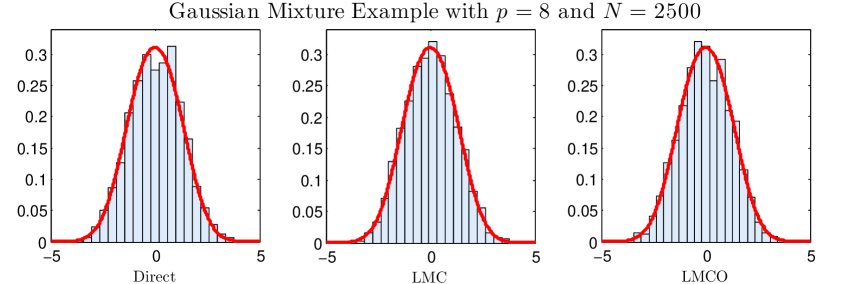
Figure 1: Histograms of the 1D projections of the samples computed using the Direct (left plot), LMC (middle plot) and LMCO (right plot) algorithms in the example of a Gaussian mixture (26). The dimension is $p=8$, the target precision is $\epsilon=0.1$ and $N=2500$ independent samples were drawn according to each of three methods. The result shows that both the LMC and the LMCO are very accurate, nearly as accurate as the direct method.

In the experiment depicted in Figure 1 (see also Table 2), we chose $\epsilon=0.1$ and, for dimensions $p\in\{4,8,12,16,20,30,40,60\}$, generated vectors using, respectively, the direct method, the LMC algorithm and the LMCO algorithm. Let $\boldsymbol{\vartheta}^{{\rm direct},i}$, $\boldsymbol{\vartheta}^{{\rm LMC},i}$ and $\boldsymbol{\vartheta}^{{\rm LMCO},i}$, $i=1,\ldots,N$, be the vectors obtained after $N$ repetitions of this experiment. In Figure 1, we plotted the histograms of the one-dimensional projections $\boldsymbol{v}^{\top}\boldsymbol{\vartheta}^{{\rm direct},i}$, $\boldsymbol{v}^{\top}\boldsymbol{\vartheta}^{{\rm LMC},i}$ and $\boldsymbol{v}^{\top}\boldsymbol{\vartheta}^{{\rm LMCO},i}$ of the sampled vectors onto the direction $\boldsymbol{v}=\mathbf{a}/\|\mathbf{a}\|_{2}$ in $\mathbb{R}^{p}$ determined by the vector $\mathbf{a}$. In order to provide a qualitative measure of accuracy of the obtained samples, we added to each histogram the curve of the true density. The latter can be computed analytically and is equal to a mixture with equal weights of two one-dimensional Gaussian densities. The result shows that both the LMC and the LMCO are very accurate, nearly as accurate as the direct method.

To illustrate the dependence on the dimension $p$ of the computational complexity of the proposed sampling strategies, we report in Table 2 the number of iterations and the overall running times for generating $N=10^{3}$ independent samples by the LMC and the LMCO for the target specified by (26), when the dimension $p$ varies in $\{4,8,12,16,20,30,40,60\}$. One may observe that the computational time is much smaller for the LMCO than for the LMC algorithm, which is mainly explained by the fact that the singular vectors of the Hessian of the function $f$, in the example under consideration, do not depend on the value $\boldsymbol{x}$ at which the Hessian is computed.

This example confirms our theoretical findings in that it shows that (a) the samples drawn from the LMC and the LMCO algorithms with the parameters $T$ and $h$ suggested by theoretical considerations have distributions that are very close to the target distribution and that (b) the running-times for these algorithms remain reasonable even for moderately large values of dimension $p$.

Example 2: Binary logistic regression

Let us consider the problem of logistic regression, in which an iid sample $\{(\boldsymbol{X}_{i},Y_{i})\}_{i=1,\ldots,n}$ is observed, with features $\boldsymbol{X}_{i}\in\mathbb{R}^{p}$ and binary labels $Y_{i}\in\{0,1\}$. The goal is to estimate the conditional distribution of $Y_{1}$ given $\boldsymbol{X}_{1}$, which amounts to estimating the regression function $r(\boldsymbol{x})=\mathbf{E}[Y_{1}|\boldsymbol{X}_{1}=\boldsymbol{x}]=\mathbf{P}(Y_{1}=1|\boldsymbol{X}_{1}=\boldsymbol{x})$. In the model of logistic regression, the regression function $r(\boldsymbol{x})$ is approximated by a logistic function of the form $r(\boldsymbol{\theta},\boldsymbol{x})=e^{\boldsymbol{\theta}^{\top}\boldsymbol{x}}/(1+e^{\boldsymbol{\theta}^{\top}\boldsymbol{x}})$. The Bayesian approach for estimating the parameter $\boldsymbol{\theta}$ relies on introducing a prior probability density on $\boldsymbol{\theta}$, $\pi_{0}(\cdot)$, and by computing the posterior density $\pi(\cdot)$. Choosing a Gaussian prior $\pi_{0}$ with zero mean and covariance matrix proportional to the inverse of the Gram matrix $\boldsymbol{\Sigma}_{\mathbf{X}}=\frac{1}{n}\sum_{i=1}^{n}\boldsymbol{X}_{i}\boldsymbol{X}_{i}^{\top}$, the posterior density takes the form

$$\pi(\boldsymbol{\theta})\propto\exp\Big{\{}-\boldsymbol{Y}^{\top}\mathbf{X}\boldsymbol{\theta}-\sum_{i=1}^{n}\log(1+e^{-\boldsymbol{\theta}^{\top}\boldsymbol{X}_{i}})-\frac{\lambda}{2}\|\boldsymbol{\Sigma}_{\mathbf{X}}^{1/2}\boldsymbol{\theta}\|_{2}^{2}\Big{\}},$$ (27)

where $\boldsymbol{Y}=(Y_{1},\ldots,Y_{n})^{\top}\in\{0,1\}^{n}$ and $\mathbf{X}$ is the $n\times p$ matrix having the feature $\boldsymbol{X}_{i}$ as $i^{\rm th}$ row. The first two terms in the exponential correspond to the log-likelihood of the logistic model, whereas the last term comes from the log-density of the prior and can be seen as a penalty term. The parameter $\lambda>0$ is usually specified by the practitioner. Many authors have studied this model from a Bayesian perspective, see for instance (Holmes and Held, 2006; Roy, 2012), and it seems that there is no compelling alternative to the MCMC algorithms for computing the Bayesian estimators in this model. Furthermore, even for the MCMC approach, although geometric ergodicity under some strong assumptions is established, there is no theoretically justified rule for assessing the convergence and, especially, ensuring that the convergence is achieved in polynomial time. Such guarantees are provided by our results, when either the LMC or the LMCO is used.

If we define the function $f$ by

$$f(\boldsymbol{\theta})=\boldsymbol{Y}^{\top}\mathbf{X}\boldsymbol{\theta}+\sum_{i=1}^{n}\log(1+e^{-\boldsymbol{\theta}^{\top}\boldsymbol{X}_{i}})+\frac{\lambda}{2}\|\boldsymbol{\Sigma}_{\mathbf{X}}^{1/2}\boldsymbol{\theta}\|_{2}^{2},$$ (28)

we get the setting described in the Introduction. It is useful here to apply the preconditioning technique of Section 4.2 with the preconditioner $\mathbf{A}=\boldsymbol{\Sigma}_{\mathbf{X}}^{-1/2}$. Thus, the LMC and the LMCO can be used with the function $f$ replaced by $g(\boldsymbol{\theta})=f(\mathbf{A}\boldsymbol{\theta})$. One checks that $g$ and $f$ are infinitely differentiable and

$$\nabla f(\boldsymbol{\theta}) =\mathbf{X}^{\top}\boldsymbol{Y}-\sum_{i=1}^{n}\frac{\boldsymbol{X}_{i}}{1+e^{\boldsymbol{\theta}^{\top}\boldsymbol{X}_{i}}}+\lambda\boldsymbol{\Sigma}_{\mathbf{X}}\boldsymbol{\theta},\quad\nabla^{2}f(\boldsymbol{\theta})=\sum_{i=1}^{n}\frac{e^{\boldsymbol{\theta}^{\top}\boldsymbol{X}_{i}}}{(1+e^{\boldsymbol{\theta}^{\top}\boldsymbol{X}_{i}})^{2}}\boldsymbol{X}_{i}\boldsymbol{X}_{i}^{\top}+\lambda\boldsymbol{\Sigma}_{\mathbf{X}}.$$

For the function $g$, since $\nabla^{2}g(\boldsymbol{\theta})=\mathbf{A}\nabla^{2}f(\mathbf{A}\boldsymbol{\theta})\mathbf{A}$, we can infer from these relations that (1) holds with $m_{\mathbf{A}}=\lambda$ and $M_{\mathbf{A}}=\lambda+0.25n$. Note here that if we do not use any preconditioner, the constants $m$ and $M$ would be given by $m=\lambda\cdot\nu_{\min}(\boldsymbol{\Sigma}_{\mathbf{X}})$ and $M=(\lambda+0.25n)\cdot\nu_{\max}(\boldsymbol{\Sigma}_{\mathbf{X}})$, where $\nu_{\min}(\boldsymbol{\Sigma})$ and $\nu_{\max}(\boldsymbol{\Sigma})$ are respectively the smallest and the largest eigenvalues of $\boldsymbol{\Sigma}$. This implies that the ratio $\nu_{\max}(\boldsymbol{\Sigma}_{\mathbf{X}})/\nu_{\min}(\boldsymbol{\Sigma}_{\mathbf{X}})$ quantifies the gain of efficiency obtained by preconditioning. This ratio might be large especially when $p$ is large and the covariates are strongly correlated.

Furthermore, $\nabla^{2}g$ is Lipschitz with a constant $L_{g}$ provided by the following formula (the proof of which is postponed to Section 8):

$$L_{g}=0.1\Big{\|}\sum_{i=1}^{n}\|\mathbf{A}\boldsymbol{X}_{i}\|_{2}\mathbf{A}\boldsymbol{X}_{i}\boldsymbol{X}_{i}^{\top}\mathbf{A}\Big{\|}\leq 0.1n\max_{i=1,\ldots,n}\|\boldsymbol{\Sigma}_{\mathbf{X}}^{-1/2}\boldsymbol{X}_{i}\|_{2}.$$ (29)

In our second experiment, for a set of values of $p$ and $n$, we randomly drew $n$ iid samples $(\boldsymbol{X}_{i},Y_{i})$ according to the following data generating device. The features $\boldsymbol{X}_{i}$ were drawn from a Rademacher distribution (i.e., each coordinate takes the values $\pm 1$ with probability $1/2$), and then renormalised to have an Euclidean norm equal to one. Each label $Y_{i}$, given $\boldsymbol{X}_{i}=\boldsymbol{x}$, was drawn from a Bernoulli distribution with parameter $r({\boldsymbol{\theta}^{\rm true}},\boldsymbol{x})$. The true vector $\boldsymbol{\theta}^{\rm true}$ was set to ${\bf 1}_{p}=(1,1,\ldots,1)^{\top}$. For each value of $p$ and $n$, we generated $100$ samples $(\mathbf{X},\boldsymbol{Y})$. For each sample, we computed the MLE using the gradient descent as described in Theorem 1 with a precision level $\epsilon=10^{-6}$. Following the recommendation of (Hanson et al., 2014), the parameter $\lambda$ was set to $3p/\pi^{2}$. We carried out two sub-experiments with well specified distinct purposes: to empirically assess the gain obtained by applying the trick of strong-convexification described in Subsection 4.3 and to evaluate the loss of accuracy caused by applying to the LMCO algorithm the second-order approximation (25).

Table 3: Example 2 (Binary logistic regression): Number of iterates using the LMC algorithm ($K$) and its modified version as described in Subsection 4.3 ($K^{\prime}$).

$\epsilon=0.1$ $n=500$ $n=1000$ $n=2000$ $n=4000$ $n=8000$ $p=2$ $K$ $0.065\times 10^{7}$ $0.137\times 10^{7}$ $0.286\times 10^{7}$ $0.596\times 10^{7}$ $1.236\times 10^{7}$ $K^{\prime}$ $2.823\times 10^{2}$ $0.688\times 10^{2}$ $0.230\times 10^{2}$ $0.089\times 10^{2}$ $0.039\times 10^{2}$ $p=5$ $K$ $0.358\times 10^{6}$ $0.751\times 10^{6}$ $1.568\times 10^{6}$ $3.257\times 10^{6}$ $6.742\times 10^{6}$ $K^{\prime}$ $4.207\times 10^{4}$ $0.222\times 10^{4}$ $0.029\times 10^{4}$ $0.007\times 10^{4}$ $0.003\times 10^{4}$ $p=20$ $K$ $0.135\times 10^{6}$ $0.279\times 10^{6}$ $0.579\times 10^{6}$ $1.201\times 10^{6}$ $2.481\times 10^{6}$ $K^{\prime}$ $0.121\times 10^{6}$ $0.250\times 10^{6}$ $0.519\times 10^{6}$ $1.075\times 10^{6}$ $2.222\times 10^{6}$ $\epsilon=0.01$ $n=500$ $n=1000$ $n=2000$ $n=4000$ $n=8000$ $p=2$ $K$ $0.151\times 10^{9}$ $0.313\times 10^{9}$ $0.645\times 10^{9}$ $1.324\times 10^{9}$ $2.714\times 10^{9}$ $K^{\prime}$ $1.529\times 10^{5}$ $0.248\times 10^{5}$ $0.077\times 10^{5}$ $0.028\times 10^{5}$ $0.011\times 10^{5}$ $p=5$ $K$ $0.075\times 10^{9}$ $0.155\times 10^{9}$ $0.320\times 10^{9}$ $0.657\times 10^{9}$ $1.345\times 10^{9}$ $K^{\prime}$ $3.652\times 10^{7}$ $0.087\times 10^{7}$ $0.011\times 10^{7}$ $0.002\times 10^{7}$ $0.001\times 10^{7}$ $p=20$ $K$ $0.254\times 10^{8}$ $0.518\times 10^{8}$ $1.062\times 10^{8}$ $2.177\times 10^{8}$ $4.459\times 10^{8}$ $K^{\prime}$ $0.227\times 10^{8}$ $0.463\times 10^{8}$ $0.947\times 10^{8}$ $1.941\times 10^{8}$ $3.975\times 10^{8}$

In the first sub-experiment, we applied the strategy outlined in Subsection 4.3 for various values of $n,p$ and $\epsilon$. To this end, we exploited the following formulae

$$m_{R} =\lambda+\nu_{\min}(\mathbf{B}_{R}),\quad\text{with}\quad\mathbf{B}_{R}:=\sum_{i=1}^{n}\frac{e^{|\boldsymbol{X}_{i}^{\top}\mathbf{A}\boldsymbol{\theta}^{*}|+R\|\mathbf{A}\boldsymbol{X}_{i}\|_{2}}}{(1+e^{2|\boldsymbol{X}_{i}^{\top}\mathbf{A}\boldsymbol{\theta}^{*}|+2R\|\mathbf{A}\boldsymbol{X}_{i}\|_{2}})^{2}}\mathbf{A}\boldsymbol{X}_{i}\boldsymbol{X}_{i}^{\top}\mathbf{A},$$

$$(p\mu_{R})^{2} =\frac{2(M/2)^{p/2}}{(m_{R}R^{2})^{p+4}\Gamma(p/2)}\sum_{j=0}^{4}C_{4}^{j}(-m_{R}R^{2})^{j}\Gamma(p+4-j;m_{R}R^{2}),$$

where $\Gamma(p;x)=\int_{x}^{\infty}t^{p-1}e^{-t}\,dt$ is the upper incomplete gamma function and $C_{4}^{j}$ stands for the binomial coefficient. The proof of the fact that the quantities $m_{R}$ and $\mu_{R}$ defined by these formulae satisfy all the assumptions of Subsection 4.3 is provided in the supplementary material. In this experiment, we used two values of $\epsilon$ ($0.1$ and $0.01$), three values of dimension $p$ ($2$, $5$ and $20$), and five values for the sample size $n$ (500, 1000, 2000, 4000 and 8000). We reported in Table 3 the number of iterates using the LMC algorithm ($K$) and the average number of iterates of the modified LMC algorithm as described in Subsection 4.3 ($K^{\prime}$). Note that in the case of modified LMC algorithm, the number of iterates depends on the original data $(\mathbf{X},\boldsymbol{Y})$. Therefore, the numbers $K^{\prime}$ reported in Table 3 are those obtained by averaging over 100 independent trials.

The results of Table 3 show clearly the advantage of using the strong-convexification trick. For instance, when $\epsilon=0.1$, $p=5$ and $n=1000$, the gain is very impressive since the number of iterations is reduced from nearly $7.5\times 10^{5}$ to $2.2\times 10^{3}$. This represents a reduction by a factor close to 340. The gain is less significant in the case when the ratio $p/n$ is larger. Our explanation of this phenomenon is that for a small ratio $p/n$, the posterior density has a very strong peak at its mode. Therefore, even for a relatively large radius $R$ the condition number $M/m_{R}$ is not too large. Thus, small $p/n$ is the typical situation in which the strong-convexification trick is likely to lead to considerable savings in running-time.

In the second sub-experiment, we aimed at verifying the validity of the second-order approximation of the LMCO algorithm, hereafter referred to as LMCO’, obtained by applying the update rule (25). To this end, for $\epsilon=0.1$, $p\in\{2,5,10\}$ and for $n\in\{200,300,400,500\}$, we generated $N_{\text{MC}}=100$ Monte-Carlo samples using the LMC algorithm and the LMCO’ algorithm. To check the closeness of the distributions of these two $p$-dimensional samples, we compared several aspects of them. More precisely, we compared their marginal means, marginal medians and marginal quartiles. Mathematically speaking, for each data-set $\mathcal{D}_{\text{data}}=(\mathbf{X},\boldsymbol{Y})$, we generated $N_{\text{MC}}$ samples $\mathcal{D}_{\text{MC}}=\{\boldsymbol{\theta}^{1},\ldots,\boldsymbol{\theta}^{N_{\text{MC}}}\}$ and $\bar{\mathcal{D}}_{\text{MC}}=\{\bar{\boldsymbol{\theta}}^{1},\ldots,\bar{\boldsymbol{\theta}}^{N_{\text{MC}}}\}$ using the LMC and the LMCO’, respectively. We then computed the normalised distance between their marginal means: $d_{\text{mean}}=\frac{1}{p}\|\mathop{\rm mean}(\mathcal{D}_{\text{MC}})-\mathop{\rm mean}(\bar{\mathcal{D}}_{\text{MC}})\|_{1}$. We also computed the quantities $d_{\rm median}$, $d_{Q_{1}}$ and $d_{Q_{3}}$, which are defined analogously by replacing the mean by the coordinate-wise median, first quartile and third quartile, respectively. The idea for considering these quantities is that, for large $N_{\rm MC}$ and small $\epsilon$, all the aforementioned distances should be close to zero.

We opted for the boxplot representation of 100 values of each of these distances obtained over 100 independent replications of the data-set $\mathcal{D}_{\text{data}}$. These boxplots are drawn in Fig. 2. They show that the distances are small—at most of the order of $10^{-1}$—which may be considered as an argument in favor of the modification proposed in (25). Indeed, with $\epsilon=0.1$ and $N_{\rm MC}=100$, we could not expect to have an error of smaller order. This is very promising since this modified LMCO algorithm has a significantly smaller computational complexity than the original LMCO: each iteration has a worst-case accuracy $O(p^{2})$ instead of $O(p^{3})$, thanks to the fact that matrix exponentials as well as the inversion of the Hessian are replaced by the computation of the Hessian and its product with vectors.

Figure 2: Boxplots of the second sub-experiment carried out within the model of logistic regression.

7 Summary and conclusion

We have established easy-to-implement, nonasymptotic theoretical guarantees for approximate sampling from log-concave and strongly log-concave probability densities. To this end, we have analysed the Langevin Monte Carlo (LMC) algorithm and its Ozaki discretised version LMCO. These algorithms can be regarded as the natural counterparts—when the task of optimisation is replaced by the task of sampling—of the gradient descent algorithm, widely studied in convex optimisation. Despite its broad applicability in the framework of Bayesian statistics and beyond, to the best of our knowledge, there were no theoretical result in the literature proving that the computational complexity of the aforementioned algorithms scales at most polynomially in dimension and in $\epsilon^{-1}$, the inverse of the desired precision level. The results proved in the present work fill this gap by showing that in order to achieve a precision (in total variation) bounded from above by $\epsilon$, the LMC needs no more than $O\big{(}\epsilon^{-2}(p^{3}+p\log(\epsilon^{-1}))\big{)}$ evaluations of the gradient when the target density is strongly log-concave and $O\big{(}\epsilon^{-4}p^{5}\log^{2}(p\vee\epsilon^{-1}))\big{)}$ evaluations of the gradient when the target density is nonstrongly log-concave. Further improvement of the rates can be achieved if a “warm start” is available. More precisely, if there is an efficiently samplable distribution $\nu$ such that the chi-squared divergence between $\nu$ and the target scales polynomially in $p$, then the LMC with an initial value drawn from $\nu$ needs no more than $O\big{(}\epsilon^{-2}p\log^{2}(p\vee\epsilon^{-1}))\big{)}$ evaluations of the gradient when the target density is strongly log-concave and $O\big{(}\epsilon^{-4}p^{3}\log^{2}(p\vee\epsilon^{-1}))\big{)}$ gradient evaluations when the target density is nonstrongly log-concave. An important advantage of our results is that all the bounds come with explicit numerical constants of reasonable magnitude.

The search for tractable theoretical guarantees for MCMC algorithms is an active topic of research not only in probability and statistics but also in theoretical computer science and in machine learning. To the best of our knowledge, first computable bounds on the constants involved in the geometric convergence of Markov chains were derived in (Meyn and Tweedie, 1994), see also subsequent work (Rosenthal, 2002; Douc et al., 2004) and the survey paper (Roberts and Rosenthal, 2004). However, because of the broad generality of the considered Markov processes, their results are difficult to implement for getting tight bounds on the constants in the context of high dimensionality. In particular, we did not succeed in deriving from their results convergence rates for the LMC algorithm (neither for its Metropolis-Hastings-adjusted version, MALA) that are polynomial in the dimension $p$ and hold for every strongly log-concave target density. Note also that some nonasymptotic convergence results for the MALA were obtained by Bou-Rabee and Hairer (2013), where strongly log-concave four times continuously differentiable functions $f$ were considered. Unfortunately, the constants involved in their bounds are not explicit and cannot be used for our purposes.

The problem of sampling from log-concave distributions is not new. It has been considered in early references (Frieze et al., 1994) and (Frieze and Kannan, 1999). An important progress in this topic was made in a series of papers by Lovázs and Vempala (see, in particular, Lovász and Vempala (2006b, a) for the sharpest results), which are perhaps the closest to our work. They investigated the problem of sampling from a log-concave density with a compact support and derived nonasymptotic bounds on the number of steps that are sufficient for approximating the target density; the best bounds are obtained for the hit-and-run algorithm. The analysis they carried out is very different from the one presented in the present work and the constants in their results are prohibitively large (for instance, $10^{31}$ in (Lovász and Vempala, 2006b, Corollary 1.2)), which makes the established guarantees of little interest for practice. On the positive side, one of the most remarkable features of the results proved in (Lovász and Vempala, 2006b, a) is that the number of steps required to achieve the level $\epsilon$ scales polylogarithmically in $1/\epsilon$. This is of course much better than the dependence on $\epsilon$ in our bounds. However, the logarithm of $1/\epsilon$ in their result is raised to power $5$, which for most interesting values of $\epsilon$ behaves itself as a linear function of $1/\epsilon$. On the down side, the dependence on the dimension in the results of Lovász and Vempala (2006b, a), when no warm start is available, scales as $p^{4}$, which is worse than $p^{3}$ inferred from our analysis. A difference worth being stressed between our framework and that of Lovász and Vempala (2006b, a) is that the LMC algorithm we have analysed here is based on the evaluations of the gradient of $f$, whereas the algorithms studied in (Lovász and Vempala, 2006b, a) need to sample from the restriction of $\pi_{f}$ on the lines. On a related note, building on the results by Lovàzs and Vempala, Belloni and Chernozhukov (2009) provided polynomial guarantees for sampling from a distribution which converges asymptotically to a Gaussian one.

After the submission of the present paper, the manuscript (Durmus and Moulines, 2015) has been posted on arXiv, which refines our results in various directions. In particular, the authors of that manuscript manage to assess more accurately the impact of the initial distribution on the final precision of the LMC algorithm and investigate an Euler scheme with nonconstant step-size. Roughly speaking, they prove that the rate we obtained in the case of a warm start is valid for any starting point which is not too far away from the mode of the density. On a related note, we focus in the present work only on the total variation distance between some MCMC algorithms and the target distribution, whereas in many applications one may be only interested in approximating integrals with respect to the target distribution. Clearly, guarantees on the total variation distance imply guarantees on the approximations of integrals, at least when the integrands are bounded functions. However, since the problem of approximating integrals is, in some sense, easier than sampling from a distribution, one could hope to get tighter bounds for the former problem. This and related questions are thoroughly investigated in (Durmus and Moulines, 2015).

Although the main contribution of the present work is of theoretical nature, we can also draw some conclusions which might be of interest for practitioners. First of all, our results show that the heuristic choice of the stopping rule for the MCMC algorithms is not the only possible option: it is also possible to have theoretically grounded guidelines for choosing the stopping time. The resulting algorithm will be of polynomial complexity both in dimension and in the precision level. Second, the results reported in this work show that there is no need to apply Metropolis-Hastings correction to the Langevin algorithm and its various variants in order to ensure their convergence. Third, when the dimension is not very high and a high level of precision is required (i.e., when $p^{3/2}\epsilon$ is small), the LMCO algorithm is preferable to the LMC algorithm, and the modified LMCO using the update rule of Eq. (25) is even better. Note, however, that this last claim was checked empirically but comes without any theoretical justification.

Finally, we would like to mention that, in recent years, several studies making the connection between convex optimisation and MCMC algorithms were carried out. They mainly focused on proposing new algorithms of approximate sampling (Girolami and Calderhead, 2011; Schreck et al., 2013; Pereyra, 2014) inspired by the ideas coming from convex optimisation. We hope that the present work will stimulate a more extensive investigation of the relationship between approximate sampling and optimisation, especially in the aim of establishing user friendly theoretical guarantees for the MCMC algorithms.

8 Postponed proofs and some technical results

8.1 Auxiliary results

Lemma 4 (Lemma 1.2.3 in Nesterov (2004)).

If the function $f$ satisfies the second inequality in (1), then $f(\boldsymbol{\theta})-f(\bar{\boldsymbol{\theta}})-\nabla f(\bar{\boldsymbol{\theta}})^{\top}(\boldsymbol{\theta}-\bar{\boldsymbol{\theta}})\leq\frac{M}{2}\|\boldsymbol{\theta}-\bar{\boldsymbol{\theta}}\|_{2}^{2}$, $\forall\boldsymbol{\theta},\bar{\boldsymbol{\theta}}\in\mathbb{R}^{p}$.

Lemma 5.

Let us denote by $\nu_{h,\boldsymbol{x}}$ the conditional density of $\boldsymbol{\vartheta}^{(1,h)}$ given $\boldsymbol{\vartheta}^{(0)}=\boldsymbol{x}$, where the sequence $\{\boldsymbol{\vartheta}^{(k,h)}\}_{k\in\mathbb{N}}$ is defined by (5) with a function $f$ satisfying (1). (In other terms, $\nu_{h,\boldsymbol{x}}$ is the density of the Gaussian distribution $\mathcal{N}(\boldsymbol{x}-h\nabla f(\boldsymbol{x}),2h\mathbf{I}_{p})$.) If $h\leq 1/(2M)$ then

$$\mathbf{E}_{\pi}\bigg{[}\frac{\nu_{h,\boldsymbol{x}}(\boldsymbol{\vartheta})^{2}}{\pi(\boldsymbol{\vartheta})^{2}}\bigg{]}\leq\exp\bigg{\{}\frac{1}{2m}\|\nabla f(\boldsymbol{x})\|_{2}^{2}-\frac{p}{2}\log(2hm)\bigg{\}}.$$

Proof.

In view of the relations

$$\pi(\boldsymbol{\theta})^{-1} =e^{f(\boldsymbol{\theta})}\int_{\mathbb{R}^{p}}e^{-f(\bar{\boldsymbol{\theta}})}\,d\bar{\boldsymbol{\theta}}=e^{f(\boldsymbol{\theta})-f(\boldsymbol{x})}\int_{\mathbb{R}^{p}}e^{-f(\bar{\boldsymbol{\theta}})+f(\boldsymbol{x})}\,d\bar{\boldsymbol{\theta}}$$

$$\leq e^{\nabla f(\boldsymbol{x})^{\top}(\boldsymbol{\theta}-\boldsymbol{x})+\frac{M}{2}\|\boldsymbol{\theta}-\boldsymbol{x}\|_{2}^{2}}\int_{\mathbb{R}^{p}}e^{-\nabla f(\boldsymbol{x})^{\top}(\bar{\boldsymbol{\theta}}-\boldsymbol{x})-\frac{m}{2}\|\bar{\boldsymbol{\theta}}-\boldsymbol{x}\|_{2}^{2}}\,d\bar{\boldsymbol{\theta}}$$

$$\leq\bigg{(}\frac{2\pi}{m}\bigg{)}^{p/2}\exp\Big{\{}{\nabla f(\boldsymbol{x})^{\top}(\boldsymbol{\theta}-\boldsymbol{x})+\frac{M}{2}\|\boldsymbol{\theta}-\boldsymbol{x}\|_{2}^{2}+\frac{1}{2m}\|\nabla f(\boldsymbol{x})\|_{2}^{2}}\Big{\}}$$

we have

$$\mathbf{E}_{\pi}\bigg{[}\frac{\nu_{h,\boldsymbol{x}}(\boldsymbol{\vartheta})^{2}}{\pi(\boldsymbol{\vartheta})^{2}}\bigg{]} =(4\pi h)^{-p}\int_{\mathbb{R}^{p}}\exp\Big{\{}-\frac{1}{2h}\;\|\boldsymbol{\theta}-\boldsymbol{x}+h\nabla f(\boldsymbol{x})\|_{2}^{2}\Big{\}}\,\pi(\boldsymbol{\theta})^{-1}\,d\boldsymbol{\theta}$$

$$\leq(4\pi h)^{-p}(2\pi/m)^{p/2}e^{\frac{1}{2m}\|\nabla f(\boldsymbol{x})\|_{2}^{2}}\int_{\mathbb{R}^{p}}\exp\Big{\{}-\frac{(1-hM)\|\boldsymbol{\theta}-\boldsymbol{x}\|_{2}^{2}}{2h}\Big{\}}\,d\boldsymbol{\theta}$$

$$=(4\pi h)^{-p}(2\pi/m)^{p/2}(2\pi h)^{p/2}(1-hM)^{-p/2}e^{\frac{1}{2m}\|\nabla f(\boldsymbol{x})\|_{2}^{2}}.$$

After a suitable rearrangement of the terms we get the claim of Lemma 5. ∎

8.2 Proofs of results concerning the LMC

Instead of proving Proposition 1, we prove below the following stronger result.

Proposition 3.

Let the function $f$ be continuously differentiable on $\mathbb{R}^{p}$ and satisfy (1) with $f^{*}=\inf_{\boldsymbol{x}\in\mathbb{R}^{p}}f(\boldsymbol{x})$. Then, for every $h\leq 1/M$, we have

$$\mathbf{E}\big{[}f(\boldsymbol{\vartheta}^{(k,h)})-f^{*}\big{]} \leq(1-mh)^{k}\mathbf{E}\big{[}f(\boldsymbol{\vartheta}^{(0)})-f^{*}\big{]}+\frac{Mp}{m(2-Mh)},$$ (30)

$$\mathbf{E}\big{[}\|\boldsymbol{\vartheta}^{(k,h)}-\boldsymbol{\theta}^{*}\|_{2}^{2}\big{]} \leq\frac{Me^{-mhk}}{m}\mathbf{E}\big{[}\|\boldsymbol{\vartheta}^{(0)}-\boldsymbol{\theta}^{*}\|_{2}^{2}\big{]}+\frac{2Mp}{m^{2}(2-Mh)}.$$ (31)

Proof.

Throughout this proof, we use the shorthand notation $f^{(k)}=f(\boldsymbol{\vartheta}^{(k,h)})$ and $\nabla f^{(k)}=\nabla f(\boldsymbol{\vartheta}^{(k,h)})$. In view of the relation (5) and the Taylor expansion, we have

$$f^{(k+1)} \leq f^{(k)}+(\nabla f^{(k)})^{\top}(\boldsymbol{\vartheta}^{(k+1,h)}-\boldsymbol{\vartheta}^{(k,h)})+\frac{M}{2}\|\boldsymbol{\vartheta}^{(k+1,h)}-\boldsymbol{\vartheta}^{(k,h)}\|_{2}^{2}$$

$$=f^{(k)}-h\|\nabla f^{(k)}\|_{2}^{2}+\sqrt{2h}\;(\nabla f^{(k)})^{\top}\boldsymbol{\xi}^{(k+1)}+\frac{M}{2}\|h\nabla f^{(k)}-\sqrt{2h}\;\boldsymbol{\xi}^{(k+1)}\|_{2}^{2}.$$

Taking the expectations of both sides, we get

$$\mathbf{E}\big{[}f^{(k+1)}\big{]} \leq\mathbf{E}\big{[}f^{(k)}\big{]}-h\mathbf{E}\big{[}\|\nabla f^{(k)}\|_{2}^{2}\big{]}+\frac{M}{2}h^{2}\mathbf{E}\big{[}\|\nabla f^{(k)}\|_{2}^{2}\big{]}+Mhp$$

$$=\mathbf{E}\big{[}f^{(k)}\big{]}-\frac{1}{2}h(2-Mh)\mathbf{E}\big{[}\|\nabla f^{(k)}\|_{2}^{2}\big{]}+Mhp.$$ (32)

It is well known (see, for instance, (Boyd and Vandenberghe, 2004)) that for the global minimum $f^{*}$ of $f$ over $\mathbb{R}^{p}$, we have

$$\|\nabla f(\boldsymbol{x})\|_{2}^{2}\geq 2m\big{(}f(\boldsymbol{x})-f^{*}\big{)},\qquad\forall\boldsymbol{x}\in\mathbb{R}^{p}.$$

Applying this inequality to $\boldsymbol{x}=\boldsymbol{\vartheta}^{(k,h)}$ and combining it with (8.2), whenever $h<2/M$ we get

$$\mathbf{E}\big{[}f^{(k+1)}\big{]} \leq\mathbf{E}\big{[}f^{(k)}\big{]}-mh(2-Mh)\mathbf{E}\big{[}f^{(k)}-f^{*}\big{]}+Mhp.$$ (33)

Let us set $\gamma=mh(2-Mh)\in(0,1)$ for any $h\in(0,2/M)$. Subtracting $f^{*}$ from the both sides of (33) we arrive at

$$\mathbf{E}\big{[}f^{(k+1)}-f^{*}\big{]} \leq(1-\gamma)\mathbf{E}\big{[}f^{(k)}-f^{*}\big{]}+Mhp.$$ (34)

This implies that

$$\mathbf{E}\big{[}f^{(k+1)}-f^{*}\big{]} \leq(1-\gamma)^{k+1}\mathbf{E}\big{[}f(\boldsymbol{\vartheta}^{(0)})-f^{*}\big{]}+Mhp(1+\ldots+(1-\gamma)^{k})$$

$$\leq(1-\gamma)^{k+1}\mathbf{E}\big{[}f(\boldsymbol{\vartheta}^{(0)})-f^{*}\big{]}+Mhp\gamma^{-1}.$$ (35)

Inequality (30) follows by replacing $\gamma$ by $mh(2-Mh)$. To prove (31), it suffices to combine (30) with the first inequality in (1), Lemma 4 and the inequality $(1-mh)^{k}\leq e^{-mhk}$. ∎

Corollary 4.

Let $h\leq 1/\alpha M$ with $\alpha\geq 1$ and $K\geq 1$ be an integer. Under the conditions of Proposition 1, it holds

$$h\sum_{k=0}^{K-1}\mathbf{E}[\|\nabla f(\boldsymbol{\vartheta}^{(k,h)})\|_{2}^{2}]\leq\frac{M\alpha}{2\alpha-1}\mathbf{E}\big{[}\|\boldsymbol{\vartheta}^{(0)}-\boldsymbol{\theta}^{*}\|_{2}^{2}\big{]}+\frac{2\alpha MKhp}{2\alpha-1}.$$

Proof.

Using inequality (8.2) and the fact that $2-Mh\geq(2\alpha-1)/\alpha$, we get

$$\frac{h(2\alpha-1)}{2\alpha}\mathbf{E}\big{[}\|\nabla f^{(k)}\|_{2}^{2}\big{]}\leq\mathbf{E}\big{[}f^{(k)}-f^{(k+1)}\big{]}+Mhp,\qquad\forall k\in\mathbb{N}.$$

Summing up these inequalities for $k=0,\ldots,K-1$ and using the obvious bound $f^{(K)}\geq f^{*}$, we get

$$h\sum_{k=0}^{K-1}\mathbf{E}\big{[}\|\nabla f^{(k)}\|_{2}^{2}\big{]}\leq\frac{2\alpha}{2\alpha-1}\mathbf{E}\big{[}f^{(0)}-f^{*}\big{]}+\frac{2\alpha MKhp}{2\alpha-1}.$$

To complete the proof, it suffices to remark that in view of Lemma 4, it holds $2\mathbf{E}\big{[}f^{(0)}-f^{*}\big{]}\leq M\mathbf{E}\big{[}\|\boldsymbol{\vartheta}^{(0)}-\boldsymbol{\theta}^{*}\|_{2}^{2}\big{]}$. ∎

Proof of Lemma 1.

The first inequality in (1) yields $\big{(}-\nabla f(\boldsymbol{\theta})+\nabla f(\bar{\boldsymbol{\theta}})\big{)}^{\top}(\boldsymbol{\theta}-\bar{\boldsymbol{\theta}})\leq-\frac{m}{2}\|\boldsymbol{\theta}-\bar{\boldsymbol{\theta}}\|_{2}^{2}$ for every $\boldsymbol{\theta},\bar{\boldsymbol{\theta}}\in\mathbb{R}^{p}$. Therefore, according to (Chen and Wang, 1997, Remark 4.14) and (Bakry et al., 2014, Corollary 4.8.2), the process $\boldsymbol{L}_{t}$ is geometrically ergodic in $L^{2}(\mathbb{R}^{p},\pi)$ that is:

$$\int_{\mathbb{R}^{p}}\big{(}\mathbf{E}\big{[}\varphi(\boldsymbol{L}_{t})|\boldsymbol{L}_{0}=\boldsymbol{x}\big{]}-\mathbf{E}_{\pi}\big{[}\varphi(\boldsymbol{\vartheta})\big{]}\big{)}^{2}\pi(\boldsymbol{x})\,d\boldsymbol{x}\leq e^{-tm}\mathbf{E}_{\pi}\big{[}\varphi^{2}(\boldsymbol{\vartheta})\big{]}$$ (36)

for every $t>0$ and every $\varphi\in L^{2}(\mathbb{R}^{p};\pi)$. The claim of the lemma follows from this inequality by simple application of the Cauchy-Schwarz inequality. Indeed, by definition of the total variation and in view of the fact that $\pi$ is the invariant density of the semigroup $\mathbf{P}^{t}_{\!\!\boldsymbol{L}}$, we have

$$\|\nu\mathbf{P}^{t}_{\!\!\boldsymbol{L}}-\pi\|_{\rm TV} =\sup_{A\in\mathscr{B}(\mathbb{R}^{p})}\bigg{|}\int_{\mathbb{R}^{p}}\mathbf{P}^{t}_{\!\!\boldsymbol{L}}(\boldsymbol{x},A)\nu(\boldsymbol{x})\,d\boldsymbol{x}-\pi(A)\bigg{|}$$

$$=\sup_{A\in\mathscr{B}(\mathbb{R}^{p})}\bigg{|}\int_{\mathbb{R}^{p}}\big{(}\mathbf{P}^{t}_{\!\!\boldsymbol{L}}(\boldsymbol{x},A)-\pi(A)\big{)}\nu(\boldsymbol{x})\,d\boldsymbol{x}\bigg{|}$$

$$=\sup_{A\in\mathscr{B}(\mathbb{R}^{p})}\bigg{|}\int_{\mathbb{R}^{p}}\big{(}\mathbf{P}^{t}_{\!\!\boldsymbol{L}}(\boldsymbol{x},A)-\pi(A)\big{)}\big{(}\nu(\boldsymbol{x})-\pi(\boldsymbol{x})\big{)}\,d\boldsymbol{x}\bigg{|}$$

$$\leq\sup_{A\in\mathscr{B}(\mathbb{R}^{p})}\int_{\mathbb{R}^{p}}\Big{|}\mathbf{P}^{t}_{\!\!\boldsymbol{L}}(\boldsymbol{x},A)-\pi(A)\Big{|}\cdot\Big{|}\frac{\nu(\boldsymbol{x})}{\pi(\boldsymbol{x})}-1\Big{|}\,\pi(\boldsymbol{x})\,d\boldsymbol{x}.$$

Using the Cauchy-Schwarz inequality, we get

$$\|\nu\mathbf{P}^{t}_{\!\!\boldsymbol{L}}-\pi\|_{\rm TV} \leq\sup_{A\in\mathscr{B}(\mathbb{R}^{p})}\bigg{(}\int_{\mathbb{R}^{p}}\big{|}\mathbf{P}^{t}_{\!\!\boldsymbol{L}}(\boldsymbol{x},A)-\pi(A)\big{|}^{2}\,\pi(\boldsymbol{x})\,dx\bigg{)}^{1/2}\chi^{2}(\nu\|\pi)^{1/2}.$$

For every fixed Borel set $A$, if we set $\varphi(\boldsymbol{x})=\mathds{1}_{A}(\boldsymbol{x})-\pi(A)$ and use (36), we obtain that

$$\int_{\mathbb{R}^{p}}\big{|}\mathbf{P}^{t}_{\!\!\boldsymbol{L}}(\boldsymbol{x},A)-\pi(A)\big{|}^{2}\,\pi(\boldsymbol{x})\,d\boldsymbol{x} =\int_{\mathbb{R}^{p}}\big{(}\mathbf{E}\big{[}\varphi(\boldsymbol{L}_{t})|\boldsymbol{L}_{0}=\boldsymbol{x}\big{]}-\mathbf{E}_{\pi}\big{[}\varphi(\boldsymbol{\vartheta})\big{]}\big{)}^{2}\,\pi(\boldsymbol{x})\,d\boldsymbol{x}$$

$$\leq e^{-tm}\mathbf{E}_{\pi}\big{[}\varphi(\boldsymbol{\vartheta})^{2}\big{]}$$

$$=e^{-tm}\pi(A)(1-\pi(A))\leq\frac{1}{4}\;e^{-tm}.$$

This completes the proof of the lemma. ∎

Proof of Lemma 2.

Setting $T=Kh$ and using (11), we get

$$\text{KL}\big{(}\mathbb{P}_{\boldsymbol{L}}^{\boldsymbol{x},T}\|\mathbb{P}_{\boldsymbol{D}}^{\boldsymbol{x},T}\big{)} =\frac{1}{4}\int_{0}^{T}\mathbf{E}\big{[}\|\nabla f(\boldsymbol{D}_{t})+\boldsymbol{b}_{t}(\boldsymbol{D})\|_{2}^{2}\big{]}\,dt$$

$$=\frac{1}{4}\sum_{k=0}^{K-1}\int_{kh}^{(k+1)h}\mathbf{E}\big{[}\|\nabla f(\boldsymbol{D}_{t})-\nabla f(\boldsymbol{D}_{kh})\|_{2}^{2}\big{]}\,dt.$$

Since $\nabla f$ is Lipschitz continuous with Lipschitz constant $M$, we have

$$\text{KL}\big{(}\mathbb{P}_{\boldsymbol{L}}^{\boldsymbol{x},T}\|\mathbb{P}_{\boldsymbol{D}}^{\boldsymbol{x},T}\big{)} \leq\frac{M^{2}}{4}\sum_{k=0}^{K-1}\int_{kh}^{(k+1)h}\mathbf{E}\big{[}\|\boldsymbol{D}_{t}-\boldsymbol{D}_{kh}\|_{2}^{2}\big{]}\,dt.$$

In view of (10) we obtain

$$\text{KL}\big{(}\mathbb{P}_{\boldsymbol{L}}^{\boldsymbol{x},T}\|\mathbb{P}_{\boldsymbol{D}}^{\boldsymbol{x},T}\big{)} \leq\frac{M^{2}}{4}\sum_{k=0}^{K-1}\int_{kh}^{(k+1)h}\Big{(}\mathbf{E}\big{[}\|\nabla f(\boldsymbol{D}_{kh})\|_{2}^{2}(t-kh)^{2}\big{]}+2p(t-kh)\Big{)}\,dt$$

$$=\frac{M^{2}h^{3}}{12}\sum_{k=0}^{K-1}\mathbf{E}\big{[}\|\nabla f(\boldsymbol{\vartheta}^{(k,h)})\|_{2}^{2}\big{]}+\frac{pKM^{2}h^{2}}{4}.$$ (37)

Applying Corollary 4, the desired inequality follows. ∎

Proof of Theorem 2.

In view of the triangle inequality, we have

$$\|\nu\mathbf{P}_{\boldsymbol{\vartheta}}^{K}-\mathbf{P}_{\pi}\|_{\rm TV} =\|\nu\mathbf{P}_{\boldsymbol{D}}^{Kh}-\mathbf{P}_{\pi}\|_{\rm TV}\leq\|{\nu}\mathbf{P}_{\boldsymbol{L}}^{T}-\mathbf{P}_{\pi}\|_{\rm TV}+\|\nu\mathbf{P}_{\boldsymbol{D}}^{T}-\nu\mathbf{P}_{\boldsymbol{L}}^{T}\|_{\rm TV}.$$ (38)

The first term in the right-hand side is what we call first type error. The source of this error is the finiteness of time, since it would be equal to zero if we could choose $T=Kh=+\infty$. The second term in the right-hand side of (38) is the second type error, which is caused by the practical impossibility to take the step-size $h$ equal to zero. These two errors can be evaluated as follows.

For the first type error, apply Lemma 1 to get $\|\nu\mathbf{P}_{\boldsymbol{L}}^{T}-\mathbf{P}_{\pi}\|_{\rm TV}\leq\frac{1}{2}\chi^{2}(\nu\|\pi)^{1/2}e^{-Tm/2}$. Since $\nu$ is a Gaussian distribution, the expectation in the above formula is not difficult to evaluate. The corresponding result, provided by Lemma 5, yields

$$\|{\nu}\mathbf{P}_{\boldsymbol{L}}^{T}-\mathbf{P}_{\pi}\|_{\rm TV} \leq\frac{1}{2}\exp\bigg{\{}\frac{p}{4}\log\bigg{(}\frac{M}{m}\bigg{)}-\frac{Tm}{2}\bigg{\}}.$$ (39)

To evaluate the second type error, we use the Pinsker inequality:

$$\|\nu\mathbf{P}_{\boldsymbol{D}}^{T}-\nu\mathbf{P}_{\boldsymbol{L}}^{T}\|_{\rm TV} \leq\|\nu\mathbb{P}_{\boldsymbol{D}}^{T}-\nu\mathbb{P}_{\boldsymbol{L}}^{T}\|_{\rm TV}\leq\Big{\{}\frac{1}{2}\text{KL}\big{(}\nu\mathbb{P}_{\boldsymbol{L}}^{T}\|\nu\mathbb{P}_{\boldsymbol{D}}^{T}\big{)}\Big{\}}^{1/2}.$$ (40)

Combining this inequality with (3), we get the desired result. ∎

8.3 Proofs of results concerning the LMCO

Proof of Theorem 3.

Using the same arguments as those of the proof of Theorem 2. This leads to the inequality

$$\big{\|}\nu\mathbf{P}_{\boldsymbol{\vartheta}}^{K}-\mathbf{P}_{\pi}\big{\|}_{\rm TV} \leq\frac{1}{2}\exp\bigg{\{}\frac{p}{4}\log\bigg{(}\frac{2M}{m}\bigg{)}-\frac{Tm}{2}\bigg{\}}+\bigg{\{}\frac{1}{2}\text{KL}\big{(}\nu\mathbb{P}_{\boldsymbol{L}}^{T}\|\nu\mathbb{P}_{\boldsymbol{D}^{O}}^{T}\big{)}\bigg{\}}^{1/2},$$ (41)

where $\mathbb{P}_{\boldsymbol{D}^{O}}^{T}$ is the probability distribution induced by the diffusion process $\boldsymbol{D}^{O}$ corresponding to the Ozaki discretisation (in fact, it is a piecewise Ornstein-Uhlenbeck process). Relation (11) implies that

$$\text{KL}\Big{(}\nu\mathbb{P}_{\boldsymbol{L}}^{T}\Big{\|}\nu\mathbb{P}_{\boldsymbol{D}^{O}}^{T}\Big{)}=\frac{1}{4}\int_{0}^{T}\mathbf{E}\Big{[}\big{\|}\nabla f(\boldsymbol{D}_{t}^{O})+b_{t}(\boldsymbol{D}^{O})\big{\|}_{2}^{2}\Big{]}\,dt.$$ (42)

Since on each interval $[kh,(k+1)h[$ the function $t\mapsto b_{t}$ is linear, for every $t\in[kh,(k+1)h[$, we get $\big{\|}\nabla f(\boldsymbol{D}_{t}^{O})+b_{t}(\boldsymbol{D}^{O})\big{\|}_{2}^{2}=\big{\|}\nabla f(\boldsymbol{D}_{t}^{O})-\nabla f(\boldsymbol{D}_{kh}^{O})-\nabla^{2}f(\boldsymbol{D}_{kh}^{O})(\boldsymbol{D}^{O}_{t}-\boldsymbol{D}_{kh}^{O})\big{\|}_{2}^{2}$. Using the mean-value theorem and the Lipschitz continuity of the Hessian of $f$, we derive from the above relation that

$$\big{\|}\nabla f(\boldsymbol{D}_{t}^{O})+b_{t}(\boldsymbol{D}^{O})\big{\|}_{2}^{2} \leq\frac{1}{4}L_{f}^{2}\big{\|}\boldsymbol{D}^{O}_{t}-\boldsymbol{D}_{kh}^{O}\big{\|}_{2}^{4},$$ (43)

for every $t\in[kh,(k+1)h[$. Note now that equation (24) provides the conditional distribution of $\boldsymbol{D}_{(k+1)h}^{O}$ given $\boldsymbol{D}_{kh}^{O}$. An analogous formula holds for the conditional distribution of $\boldsymbol{D}_{t}^{O}-\boldsymbol{D}_{kh}^{O}$ given $\boldsymbol{D}_{kh}^{O}$, which is multivariate Gaussian with mean $\big{(}\mathbf{I}_{p}-e^{-(t-kh)\mathbf{H}_{k}}\big{)}\mathbf{H}_{k}^{-1}\nabla f\big{(}\boldsymbol{D}_{kh}^{O}\big{)}$ and covariance matrix $\boldsymbol{\Sigma}_{k}=\big{(}\mathbf{I}_{p}-e^{-2(t-hk)\mathbf{H}_{k}}\big{)}\mathbf{H}_{k}^{-1}$, where $\mathbf{H}_{k}=\nabla^{2}f(\boldsymbol{D}_{kh}^{O})$. Under convexity condition on $f$, we have $\|\big{(}\mathbf{I}_{p}-e^{-s\mathbf{H}_{k}}\big{)}\mathbf{H}_{k}^{-1}\|\leq s$ for every $s>0$. Therefore, conditioning with respect to $\boldsymbol{D}_{kh}^{O}$ and using the inequality $(a+b)^{4}\leq 8(a^{4}+b^{4})$, for every $t\in[kh,(k+1)h[$ we get

$$\frac{1}{4}\mathbf{E}\big{[}\big{\|}\boldsymbol{D}^{O}_{t}-\boldsymbol{D}_{kh}^{O}\big{\|}_{2}^{4}\,\big{|}\,\boldsymbol{D}_{kh}^{O}\big{]} \leq\big{\|}\big{(}\mathbf{I}_{p}-e^{-(t-kh)\mathbf{H}_{k}}\big{)}\mathbf{H}_{k}^{-1}\nabla f\big{(}\boldsymbol{D}_{kh}^{O}\big{)}\big{\|}^{4}_{2}+\mathbf{E}\Big{[}\big{\|}\boldsymbol{\Sigma}_{k}^{1/2}\boldsymbol{\xi}^{(k+1)}\big{\|}^{4}_{2}\,\Big{|}\,\boldsymbol{D}_{kh}^{O}\Big{]}$$

$$\leq(t-hk)^{4}\big{\|}\nabla f\big{(}\boldsymbol{D}_{kh}^{O}\big{)}\big{\|}^{4}_{2}+(p+1)^{2}\big{\|}(\mathbf{I}_{p}-e^{-2(t-hk)\mathbf{H}_{k}})\mathbf{H}_{k}^{-1}\big{\|}^{2}$$

$$\leq(t-hk)^{4}\big{\|}\nabla f\big{(}\boldsymbol{D}_{kh}^{O}\big{)}\big{\|}^{4}_{2}+4(t-hk)^{2}(p+1)^{2}.$$

This inequality, in conjunction with (42) and (43) yields

$$\text{KL}\Big{(}\nu\mathbb{P}_{\boldsymbol{L}}^{T}\Big{\|}\nu\mathbb{P}_{\boldsymbol{D}^{O}}^{T}\Big{)} \leq\frac{L_{f}^{2}}{16}\sum_{k=0}^{K-1}\int_{kh}^{(k+1)h}\mathbf{E}\Big{(}\mathbf{E}\Big{[}\big{\|}\boldsymbol{D}_{t}^{O}-\boldsymbol{D}_{kh}^{O}\big{\|}_{2}^{4}\,\big{|}\boldsymbol{D}_{kh}^{O}\Big{]}\Big{)}\,dt$$

$$\leq\frac{L_{f}^{2}h^{5}}{20}\sum_{k=0}^{K-1}\mathbf{E}\big{(}\big{\|}\nabla f\big{(}\boldsymbol{D}_{kh}^{O}\big{)}\big{\|}^{4}_{2}\big{)}+\frac{1}{3}L^{2}_{f}Kh^{3}(p+1)^{2}.$$ (44)

To bound the last expectation, we use the fact that $\boldsymbol{D}_{kh}^{O}$ equals $\bar{\boldsymbol{\vartheta}}^{(k,h)}$ in distribution, and the next lemma (the proof of which is provided in the supplementary material).

Lemma 6.

If $p\geq 2$, $T\geq 4/(3M)$ and $h\leq 1/(8M)$, then the iterates of the LMCO algorithm satisfy $\mathbf{E}\big{[}\big{(}\sum_{k=0}^{K-1}\|\nabla f(\bar{\boldsymbol{\vartheta}}^{(k,h)})\|_{2}^{2}\big{)}^{2}\big{]}\leq\frac{32}{3}\big{(}{TMp}/h\big{)}^{2}$.

Combining this lemma and (8.3), we upper bound the Kullback-Leibler divergence as follows $\text{KL}\big{(}\nu\mathbb{P}_{\boldsymbol{L}}^{T}\big{\|}\nu\mathbb{P}_{\boldsymbol{D}^{O}}^{T}\big{)}\leq 0.534h^{3}(L_{f}TMp)^{2}+0.75T(L_{f}hp)^{2}$, which completes the proof. ∎

References

- Atchadé et al. (2011) Y. Atchadé, G. Fort, E. Moulines, and P. Priouret. Adaptive Markov chain Monte Carlo: theory and methods. In Bayesian time series models, pages 32–51. Cambridge Univ. Press, Cambridge, 2011.
- Bakry et al. (2014) D. Bakry, I. Gentil, and M. Ledoux. Analysis and geometry of Markov diffusion operators, volume 348 of Grundlehren der Mathematischen Wissenschaften [Fundamental Principles of Mathematical Sciences]. Springer, Cham, 2014.
- Belloni and Chernozhukov (2009) A. Belloni and V. Chernozhukov. On the computational complexity of MCMC-based estimators in large samples. Ann. Statist., 37(4):2011–2055, 2009.
- Bou-Rabee and Hairer (2013) N. Bou-Rabee and M. Hairer. Nonasymptotic mixing of the MALA algorithm. IMA J. Numer. Anal., 33(1):80–110, 2013.
- Boyd and Vandenberghe (2004) S. Boyd and L. Vandenberghe. Convex optimization. Cambridge University Press, Cambridge, 2004.
- Brooks (1998) S. P. Brooks. MCMC convergence diagnosis via multivariate bounds on log-concave densities. Ann. Statist., 26(1):398–433, 02 1998.
- Chen and Wang (1997) Mu-Fa Chen and Feng-Yu Wang. Estimation of spectral gap for elliptic operators. Trans. Amer. Math. Soc., 349(3):1239–1267, 1997.
- Dalalyan and Tsybakov (2009) A. S. Dalalyan and A. B. Tsybakov. Sparse regression learning by aggregation and langevin monte-carlo. In COLT 2009 - The 22nd Conference on Learning Theory, Montreal, June 18-21, 2009, pages 1–10, 2009.
- Dalalyan and Tsybakov (2012) A. S. Dalalyan and A. B. Tsybakov. Sparse regression learning by aggregation and Langevin Monte-Carlo. J. Comput. System Sci., 78(5):1423–1443, 2012.
- Douc et al. (2004) R. Douc, E. Moulines, and Jeffrey S. Rosenthal. Quantitative bounds on convergence of time-inhomogeneous Markov chains. Ann. Appl. Probab., 14(4):1643–1665, 2004.
- Durmus and Moulines (2015) A. Durmus and E. Moulines. Non-asymptotic convergence analysis for the unadjusted langevin algorithm. preprint, arXiv:1507.05021, 2015.
- Frieze and Kannan (1999) A. Frieze and R. Kannan. Log-Sobolev inequalities and sampling from log-concave distributions. Ann. Appl. Probab., 9(1):14–26, 1999.
- Frieze et al. (1994) A. Frieze, R. Kannan, and N. Polson. Sampling from log-concave distributions. Ann. Appl. Probab., 4(3):812–837, 1994.
- Girolami and Calderhead (2011) M. Girolami and B. Calderhead. Riemann manifold Langevin and Hamiltonian Monte Carlo methods. J. R. Stat. Soc. Ser. B Stat. Methodol., 73(2):123–214, 2011.
- Hanson et al. (2014) T. Hanson, A. Branscum, and W. Johnson. Informative -priors for logistic regression. Bayesian Anal., 9(3):597–611, 2014.
- Holmes and Held (2006) C. Holmes and L. Held. Bayesian auxiliary variable models for binary and multinomial regression. Bayesian Anal., 1(1):145–168, 2006.
- Jarner and Hansen (2000) S. F. Jarner and E. Hansen. Geometric ergodicity of Metropolis algorithms. Stochastic Process. Appl., 85(2):341–361, 2000.
- Lamberton and Pagès (2002) D. Lamberton and G. Pagès. Recursive computation of the invariant distribution of a diffusion. Bernoulli, 8(3):367–405, 2002.
- Lemaire (2005) V. Lemaire. Estimation numérique de la mesure invariante d’un processus de diffusion. PhD thesis, Université de Marne-la-Vallée, 2005.
- Lovász and Vempala (2006a) L. Lovász and S. Vempala. Hit-and-run from a corner. SIAM J. Comput., 35(4):985–1005 (electronic), 2006a.
- Lovász and Vempala (2006b) L. Lovász and S. Vempala. Fast algorithms for logconcave functions: Sampling, rounding, integration and optimization. In 47th Annual IEEE Symposium on Foundations of Computer Science (FOCS 2006), 21-24 October 2006, Berkeley, California, USA, Proceedings, pages 57–68, 2006b.
- Meyn and Tweedie (1994) S. P. Meyn and R. L. Tweedie. Computable bounds for geometric convergence rates of Markov chains. Ann. Appl. Probab., 4(4):981–1011, 1994.
- Nesterov (2004) Yu. Nesterov. Introductory lectures on convex optimization, volume 87 of Applied Optimization. Kluwer Academic Publishers, Boston, MA, 2004.
- Ozaki (1992) T. Ozaki. A bridge between nonlinear time series models and nonlinear stochastic dynamical systems: a local linearization approach. Statistica Sinica, 2(1):113–135, 1992.
- Pereyra (2014) M. Pereyra. Proximal markov chain monte carlo algorithms. Technical report, arXiv:1306.0187, 2014.
- Pillai et al. (2012) N. S. Pillai, A. M. Stuart, and A. H. Thiéry. Optimal scaling and diffusion limits for the Langevin algorithm in high dimensions. Ann. Appl. Probab., 22(6):2320–2356, 2012.
- Roberts and Rosenthal (1998) G. O. Roberts and J. S. Rosenthal. Optimal scaling of discrete approximations to Langevin diffusions. J. R. Stat. Soc. Ser. B Stat. Methodol., 60(1):255–268, 1998.
- Roberts and Rosenthal (2004) G. O. Roberts and J. S. Rosenthal. General state space markov chains and mcmc algorithms. Probab. Surveys, 1:20–71, 2004.
- Roberts and Stramer (2002) G. O. Roberts and O. Stramer. Langevin diffusions and Metropolis-Hastings algorithms. Methodol. Comput. Appl. Probab., 4(4):337–357 (2003), 2002.
- Roberts and Tweedie (1996) G. O. Roberts and R. L. Tweedie. Exponential convergence of Langevin distributions and their discrete approximations. Bernoulli, 2(4):341–363, 1996.
- Rosenthal (2002) J. S. Rosenthal. Quantitative convergence rates of Markov chains: a simple account. Electron. Comm. Probab., 7:123–128 (electronic), 2002.
- Roy (2012) V. Roy. Convergence rates for MCMC algorithms for a robust Bayesian binary regression model. Electron. J. Stat., 6:2463–2485, 2012.
- Saumard and Wellner (2014) A. Saumard and J. A. Wellner. Log-concavity and strong log-concavity: a review. Stat. Surv., 8:45–114, 2014.
- Schreck et al. (2013) A. Schreck, G. Fort, S. Le Corff, and E. Moulines. A shrinkage-thresholding metropolis adjusted langevin algorithm for bayesian variable selection. preprint, arXiv:1312.5658, 2013.
- Stramer and Tweedie (1999a) O. Stramer and R. L. Tweedie. Langevin-type models. I. Diffusions with given stationary distributions and their discretizations. Methodol. Comput. Appl. Probab., 1(3):283–306, 1999a.
- Stramer and Tweedie (1999b) O. Stramer and R. L. Tweedie. Langevin-type models. II. Self-targeting candidates for MCMC algorithms. Methodol. Comput. Appl. Probab., 1(3):307–328, 1999b.
- Xifara et al. (2014) T. Xifara, C. Sherlock, S. Livingstone, S. Byrne, and M. Girolami. Langevin diffusions and the Metropolis-adjusted Langevin algorithm. Statist. Probab. Lett., 91:14–19, 2014.