Communicability Angle
and the Spatial Efficiency of Networks

Abstract

We introduce the concept of communicability angle between a pair of nodes in a graph. We provide strong analytical and empirical evidence that the average communicability angle for a given network accounts for its spatial efficiency on the basis of the communications among the nodes in a network. We determine characteristics of the spatial efficiency of more than a hundred real-world complex networks that represent complex systems arising in a diverse set of scenarios. In particular, we find that the communicability angle correlates very well with the experimentally measured value of the relative packing efficiency of proteins that are represented as residue networks. We finally show how we can modulate the spatial efficiency of a network by tuning the weights of the edges of the networks. This allows us to predict effects of external stresses on the spatial efficiency of a network as well as to design strategies to improve important parameters in real-world complex systems.

distance; graph planarity; Euclidean distance

1 Introduction

Graphs are frequently used to represent discrete objects both in abstract mathematics and computer sciences as well as in applications, such as theoretical physics, biology, ecology and social sciences [26, 14]. In the particular case of representing the networked skeleton of complex systems, graphs receive the denomination of complex networks; we will hereafter use graphs and networks interchangeably.

Complex networks are ubiquitous in many real-world scenarios, ranging from the biomolecular — those representing gene transcription, protein interactions, and metabolic reactions — to the social and infrastructural organization of modern society [11, 36, 9]. In many of these networks, nodes and edges are used to represent physically embedded objects [4], namely spatial networks. In urban street networks, for instance, the nodes describe the intersection of streets, which are represented by the edges of the graph. These streets and their intersections are embedded in the two-dimensional space representing the surface occupied by the corresponding city [28]. Thus, these networks are planar graphs in the sense that we can draw them in a plane without edge intersections, except for the few bridges and overpasses present in a city. Another spatial network is the brain network, in which the nodes account for brain regions embedded in the three-dimensional space occupied by the brain, while the edges represent the communication or physical connections among these regions [7]. We can also capture the three-dimensional structure of proteins by means of the residue networks in which nodes describe amino acids and the edges represent physical interactions among them. Other examples include the following: infrastructures, such as the Internet, transportation networks, water and electricity supply networks, etc. [4]; anatomical networks, such as vascular and organ/tissue networks; the networks of channels in fractured rocks; the networks representing the corridors and galleries in animal nests; for even more, see Ref. [11] and references therein.

A natural question that arises in the analysis of spatial networks is how efficiently they use the available geographical space in which they are embedded. In a protein, for instance, the linear polypeptide chain is folded up into a globular shape in order to minimize the volume occupied inside the cell [10]. In airport transportation networks the nodes are embedded into the two-dimensional space represented by the surface of a country or continent, but the connections between the airports occupy the available three-dimensional space (it might be argued that they use a four-dimensional space as two flights can intersect in space but at different times), which increases the spatial efficiency of these networks. In contrast, the planarity of urban street networks [8] implies that both nodes and edges are embedded in a two-dimensional space, which in general decreases the number of alternative routes between different points in the network. This relatively poor spatial efficiency of modern cities, i.e., the non-existence of three-dimensional cities (although they have been already planned; see Chapter 3 in Ref. [11] and references therein), has posed a serious challenge to their continuous growth in view of their threat to the natural environment. Although the planarity may be an important part of this problem, it is definitively not the only one. Two planar networks, e.g., two cities, can display significantly different spatial efficiency, and the same is true for pairs of non-planar networks.

The concept of spatial efficiency is adapted here from economics, where it is frequently used to describe how much time, effort and cost a given arrangement produces for governments, businesses and households to conduct their activities as compared to alternative arrangements; see Ref. [40] and references therein. This concept has a lot to do with the efficiency in communication among the parts of the system under study and as so it is a well-posed problem for its analysis beyond spatial networks.

Indices for communication efficiency of networks have been previously proposed in the literature [30, 31, 1, 23]. They have revolved around the idea of considering the sum of reciprocal shortest-path distances in graphs. It is worth mentioning that the sum of all the reciprocal shortest-path distances in a graph is known in graph theory as the Harary index, which was introduced by Plavšić et al. in 1993 [38] and studied elsewhere [46, 45]. The so-called efficiency index introduced by Latora and Marchiori [30] (defined below in Eq. (3)) is the average Harary index of a graph. In the present work we will consider a new communication efficiency measure that takes into account all the potential routes communicating a pair of nodes instead of using the shortest paths only. The consequences of this adoption will be developed in the rest of the paper.

In this context of communication among the nodes of a network, we [16] have introduced the communicability function as a way to quantify how much information can flow from one node to another in a network; see also Refs. [17, 18]. We regard the quantity $G_{pq}$, which we will define in Eq. (2) below, as the amount of information that departs from a node $p$ and ends at a node $q$. On the other hand, we regard $G_{pp}$ as the amount of information that departs from the original node $p$ and never arrives at the destination $q$, because it is returned to its originator. Let us call the first amount of information the successful information and the second the frustrated one. Then, the goodness of communication between the two nodes is given by the ratio of the successful to the frustrated amount of information. Increasing the amount of successful information and reducing the amount of frustrated one improves the quality of communication between the two nodes. This has lead to the definition of a quantity [12, 13, 20] that has been proved to be a distance between two nodes.

In the present paper, we show a remarkable mapping of each node of a network to a point on the surface of a hypersphere. We prove that the distance defined based on the communicability function is indeed the chord distance between the two points on the hypersphere. We can thereby assign a Euclidean angle to each pair of nodes which represents the communication efficiency between them. We then analyze various networks using the angle, which we refer to as the communicability angle hereafter, and provide evidence that this angle accounts for the spatial efficiency of networks.

2 Preliminaries

In this section we shall present some of the definitions, notations, and properties associated with networks to make this work self-contained. A graph $\Gamma=(V,E)$ is defined by a set of $n$ nodes (vertices) $V$ and a set of $m$ edges (links) $E=\{(p,q)|p,q\in V\}$ between the nodes. An edge is said to be incident to a vertex $p$ if there exists a node $q(\neq p)$ such that either $(p,q)\in E$ or $(q,p)\in E$. The degree of a vertex, denoted by $k_{p}$, is the number of edges incident to $p$ in $\Gamma$. The graph is said to be undirected if the edges are formed by unordered pairs of vertices. A walk of length $\ell$ in $\Gamma$ is a set of nodes $p_{1},p_{2},\ldots,p_{\ell},p_{\ell+1}$ such that for all $1\leq i\leq\ell$, $(p_{i},p_{i+1})\in E$. A closed walk is a walk for which $p_{1}=p_{\ell+1}$. A path is a walk with no repeated nodes. A graph is connected if there is a path connecting every pair of nodes. A graph with unweighted edges, no self-loops (edges from a node to itself), and no multiple edges is said to be simple. Throughout this work, we will always consider undirected, simple, and connected networks.

More specifically, we will consider graphs which are defined as follows. The path graph $P_{n}$ is a connected graph with $n$ nodes, $n-2$ of which have degree 2 and the remaining two have degree 1. The complete graph $K_{n}$ is the graph with $n$ nodes and $n(n-1)/2$ edges. The complete bipartite graph $K_{n_{1},n_{2}}$ is the graph with $n=n_{1}+n_{2}$ nodes split into two disjoint sets, one containing $n_{1}$ nodes and the other containing $n_{2}$ nodes, while the edges connect every node in one set with every one in the other. The particular case $K_{1,n-1}$ is known as the star graph. A graph is planar if it can be drawn on a plane without any edge crossings. The following is a well-known characterization of the planar graphs known as the Kuratowski theorem (see Ref. [25]).

Theorem 1.

A network is planar if and only if it has no subgraph homeomorphic to $K_{5}$ or $K_{3,3}$.

Let us consider a matrix $A$ called the adjacency matrix, whose elements are $A_{pq}=1$ if $(p,q)\in E$ and zero otherwise. For undirected simple finite graphs, $A$ is a real symmetric matrix. We can therefore decompose it into the form

(1) $$A=U\Lambda U^{T},$$

where $\Lambda$ is a diagonal matrix containing the eigenvalues of $A$, which we label in non-increasing order $\lambda_{1}\geq\lambda_{2}\geq\ldots\geq\lambda_{n}$, and $U=[\vec{\psi}_{1},\ldots,\vec{\psi}_{n}]$ is an orthogonal matrix, where $\vec{\psi}_{\mu}$ is an eigenvector associated with $\lambda_{\mu}$. Because we consider connected graphs, $A$ is irreducible; the Perron-Frobenius theorem then dictates that $\lambda_{1}>\lambda_{2}$ and that we can choose $\vec{\psi}_{1}$ such that its components $\psi_{1}(p)$ are positive for all $p\in V$.

An important quantity for studying communication processes in networks is the communicability function [16, 18, 17], defined for each pair of nodes $p$ and $q$ as

(2) $$G_{pq}=\sum_{k=0}^{\infty}\frac{\left(A^{k}\right)_{pq}}{k!}=\left(e^{A}\right)_{pq}=\sum_{\mu=1}^{n}e^{\lambda_{\mu}}\vec{\psi}_{\mu}(p)\vec{\psi}_{\mu}(q).$$

The factor $\left(A^{k}\right)_{pq}$ counts the number of walks of length $k$ starting at the node $p$ and ending at the node $q$. The communicability function is the sum of the numbers of walks of length $k$, each weighted by the factor $1/k!$ so that shorter walks may be more influential than longer ones. In Eq. (2), the exponential of the matrix $A$ is defined by its Taylor expansion, which is the communicability function itself. The spectral decomposition on the right-hand side is also derived from the spectral decomposition of each term of the Taylor expansion: $(A^{k})_{pq}=\sum_{\mu}(\lambda_{\mu})^{k}\vec{\psi}_{\mu}(p)\vec{\psi}_{\mu}(q)$.

The importance of the communicability function (2) lies in the fact that it takes account of long walks as well as short ones; even two nodes connected by a very long shortest path can have a strong communication if they are connected by very many longer walks. The diagonal term $G_{pp}$ characterizes the degree of participation of the node $p$ in all subgraphs of the network. It is thus known as the subgraph centrality of the corresponding node [19].

We can visualize the communicability function (2) in another way. Consider a matrix-vector equation $d\vec{\psi}/dt=A\vec{\psi}$, which governs the time evolution of a vector $\vec{\psi}(t)$. If the vector $\vec{\psi}(t)$ describes a random-walker distribution on the network in question at time $t$, the above equation describes how the walkers move around on the network. Its formal solution is given by $\vec{\psi}(t)=e^{At}\vec{\psi}(0)$, and hence the exponential matrix $e^{A}$ is the time evolution operator for the unit time. Therefore, the communicability function (2) is the transition rate for the walkers on the site $p$ (represented by a vector $\vec{w}_{p}$) to move to the site $q$ (represented by another vector $\vec{w}_{q}$) after the unit time, where $w_{p}$ is a column vector with unity on the $p$th element and zero on the others.

It is possible to define several distance measures on networks. The most common one is the shortest-path or geodesic distance between two nodes $p,q\in V$, which is defined as the length of the shortest path connecting these nodes. We will write $d(p,q)$ to denote the distance between $p$ and $q$. Here we will refer to the average of the shortest-path distance in the graph as the average path length, as usual in network theory. The communication efficiency of a networks is defined on the basis of this shortest-path distance as [30]

(3) $$E=\dfrac{1}{n\left(n-1\right)}\sum_{p,q}d_{pq}^{-1},$$

where $d_{pq}=d\left(p,q\right)$. The index $H=\sum_{p,q}d_{pq}^{-1}$ is the Harary index [38] mentioned above.

Another distance measure among the nodes of a graph is the so-called resistance distance [29] which is defined by $\Omega_{pq}=L_{pp}^{+}+L_{qq}^{+}-2L_{pq}^{+}$, where $L^{+}$ is the Moore-Penrose pseudoinverse of the Laplacian matrix of the network [44, 22]; the network Laplacian is defined by $L=K-A$ with $K=\mathop{\mathrm{diag}}\left(k_{i}\right)$. The resistance distance considers not only the shortest paths but also longer walks in the communication between two nodes. In spite of the potential similarity with the communicability function (2), they exhibit very important differences. For instance, the communicability distance, a metric based on communicability function, is highly uncorrelated with the resistance distance [12]. More importantly, Luxburg et al. [33] have proved that for extremely large graphs the resistance distance converges to an expression that does not take into account the structure of the graph at all and is completely meaningless as a distance function on the graph. This situation does not occur for the communicability-based functions.

An important concept in graph theory is the isoperimetric number of the graph, which is the discrete analogous of the Cheeger constant. Let $S\subset V$, such that $0<\left|S\right|<\left|V\right|/2$. Also, let $\partial S=\left\{U\subset E\left|\left(p,q\right)\in U\implies p\in S,q\in\bar{S}\right.\right\}$ be the neighborhood of the set $S$. The isoperimetric constant is defined as

(4) $$i\left(G\right)=\underset{S}{\inf}\dfrac{\left|\partial S\right|}{\left|S\right|}.$$

A large isoperimetric number indicates that the graph lacks any structural bottlenecks, which means that the graph is super-homogeneous, lacking any holes or core-periphery structures. Formally, a graph hole, also known as a chordless cycle, is a cycle $C$ of length at least four such that no two nodes of the cycle are connected by an edge that does not itself belong to $C$.

In the next section we will introduce a third distance measure defined recently on the basis of the communicability function. It is novel in the sense that longer walks than the shortest path are taken into account.

3 Communicability distance

The new distance function is defined as [12, 13]

(5) $${\xi_{pq}}^{2}=G_{pp}+G_{qq}-2G_{pq},$$

which we will refer to as the communicability distance between the nodes $p$ and $q$ in $\Gamma$. The intuition behind it is that when two nodes $p$ and $q$ communicate with each other, the quality of their communication depends on two factors: (i) how much information departing from the node $p$ ($q$) arrives at the node $q$ ($p$), and (ii) how much information departing from the node $p$ ($q$) returns to that node $p$ ($q$) without arriving at its destination. That is, the communication efficiency increases with the amount of information which departs from the originator and arrives at its destination, but decreases with the amount of information which is frustrated due to the fact that the information returns to its originator without being delivered to its target. We can rephrase the information flow as the random walkers according to the interpretation that $e^{A}$ is a time-evolution operator for the unit time. This intuition has lead to the definition (5).

It has been indeed proved that the function $\xi_{pq}$ is a Euclidean distance between the nodes $p$ and $q$ in $\Gamma$ [12].

Theorem 3.2 [20].

The communicability distance $\xi_{pq}$ induces an embedding of the graph $\Gamma$ of size $n$ into a hypersphere of radius $R^{2}=[c-{\left(2-b\right)^{2}}/{a}]/4$ in an $\left(n-1\right)$-dimensional space, where $a=\vec{1}^{T}e^{-A}\vec{1}$, $b=\vec{s}^{T}e^{-A}\vec{1}$ and $c=\vec{s}^{T}e^{-A}\vec{s}$ with $\vec{s}=\mathop{\mathrm{diag}}e^{A}$.

Let us hereafter give a more intuitive and geometric view of the communicability distance. For the purpose, we first prove the following theorem.

Theorem 3.3.

Let $\vec{x}_{p}=e^{\Lambda/2}\vec{\phi}_{p}$, where $\vec{\phi}_{p}=\begin{pmatrix}\psi_{1}(p)&\cdots&\psi_{\mu}(p)&\cdots&\psi_{n}(p)\end{pmatrix}^{T}$. Then we have

(6) $$G_{pq}=\vec{x}_{p}\cdot\vec{x}_{q}.$$

Proof.

Let $X=\begin{pmatrix}\vec{x}_{1}&\cdots&\vec{x}_{p}&\cdots&\vec{x}_{n}\end{pmatrix}=e^{\Lambda/2}U^{T}$. We therefore have

(7) $$X^{T}X=Ue^{\Lambda}U^{T}=e^{A}=G,$$

which is immediately followed by Eq. (6). ∎

This theorem transforms the communicability distance (5) into the form

(8) $${\xi_{pq}}^{2}=\vec{x}_{p}\cdot\vec{x}_{p}+\vec{x}_{q}\cdot\vec{x}_{q}-2\vec{x}_{p}\cdot\vec{x}_{q}=\left(\vec{x}_{p}-\vec{x}_{q}\right)^{2}.$$

In other words, the communicability distance is the Euclidean distance in the space of $\{\vec{x}_{p}\}$. In order to visualize this space, let us go back to the interpretation that $(e^{A})_{pq}$ is the transition rate of the random walkers from the $p$th site to the $q$th site. An initial state $\vec{w}_{p}$ is a basis vector in the original vector space but its expression is given by $\vec{\phi}_{p}$ above in the vector space with the eigenvectors $\vec{\psi}_{\mu}$ as its basis vectors, namely the eigenspace; see Fig. 1 for an example for the path graph $P_{3}$.

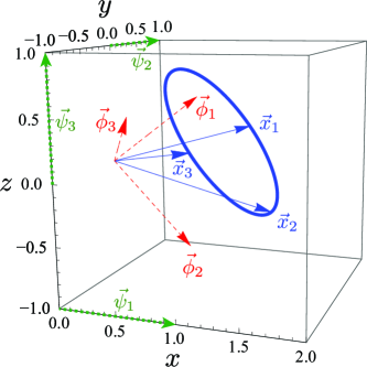
Fig. 1: A demonstration plot of $\vec{\phi}_{p}$ (red dashed arrows) and $\vec{x}_{p}$ (blue solid arrows) for the path graph $P_{3}$. The eigenvectors $\vec{\psi}_{\mu}$ (green dotted arrows) define the axes of this eigenspace. The communicability distance $\xi_{pq}$ is the chord distance on the (blue) circle that goes through the end points of the vectors $\vec{x}_{p}$.

In other words, the initial vector represents the state in which all random walkers sit on the $p$th site, but it is denoted by the vector $\vec{\phi}_{p}$ in the eigenspace. The vector $\vec{x}_{p}$ is a vector in the eigenspace, representing a state in which random walkers from the $p$th site move around for the time $1/2$.

Theorem 3.1 dictates that the vectors $\{\vec{x}_{p}\}$ fall onto the surface of a hypersphere in the space; see Fig. 2(a) for illustration in the case $n=3$.

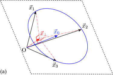
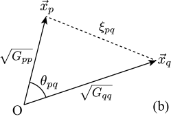
Fig. 2: (a) Three vectors $\vec{x}_{1}$, $\vec{x}_{2}$ and $\vec{x}_{3}$ (solid black arrows) in a three-dimensional space spanned by the three eigenvectors of a $3\times 3$ adjacency matrix $A$. The vectors fall on a two-dimensional flat surface (broken black lines) to which the vector $\vec{x}_{\perp}$ (red dot-dashed arrow) is normal. We can draw a circle (solid blue curve) on the two-dimensional surface around a point $\vec{x}_{0}$ (solid blue arrow) to contain all three points. (b) The triangle spanned by the vectors $\vec{x}_{p}$ and $\vec{x}_{q}$.

We can understand this in the following way. We first fix the $n$-dimensional normal vector $\vec{x}_{\perp}$ from $n$ pieces of conditions $(\vec{x}_{p}-\vec{x}_{\perp})\cdot\vec{x}_{\perp}=0$ for $1\leq p\leq n$. It specifies the $(n-1)$-dimensional flat surface on which all vectors fall as $(\vec{x}-\vec{x}_{\perp})\cdot\vec{x}_{\perp}=0$. We next fix the $n$-dimensional vector $\vec{x}_{0}$ that specifies the center of the hypersphere as well as the radius $R$ from $n+1$ pieces of conditions $(\vec{x}_{0}-\vec{x}_{\perp})\cdot\vec{x}_{\perp}=0$ and $|\vec{x}_{p}-\vec{x}_{0}|=R$ for $1\leq p\leq n$.

We can therefore regard ${\xi_{pq}}$ as the chord distance between the two points on the hypersurface. Figure 2(b) picks out the triangle spanned by the vectors $\vec{x}_{p}$ and $\vec{x}_{q}$. This leads to the definition in the next section of the angle between the two vectors.

4 Communicability angle

Let $p$ and $q$ be nodes of a connected simple network and let us define the following quantity:

(9) $$\gamma_{pq} \coloneqq\frac{G_{pq}}{\sqrt{G_{pp}G_{qq}}}.$$

We then prove the following result.

Theorem 4.4.

The index $\gamma_{pq}$ is the cosine of the Euclidean angle spanned by the position vectors of $p$ and $q$.

Proof.

The view shown in Fig. 2(b) obviously gives

(10) $$\cos\theta_{pq} =\frac{\vec{x}_{p}\cdot\vec{x}_{q}}{\left|\vec{x}_{p}\right|\left|\vec{x}_{q}\right|}.$$

The use of Eq. (6) then proves the result. ∎

We then call $\theta_{pq}$ the communicability angle between the corresponding nodes of the graph. Details on how to compute the communicability angle for networks are given in the Supplementary Information accompanying the present paper. For each pair of nodes in the graph, the communicability distance and angle are related mathematically by the following expression:

(11) $${\xi_{pq}}^{2}=G_{pp}+G_{qq}-2\sqrt{G_{pp}G_{qq}}\cos\theta_{pq}.$$

Because $G_{pq}\geq 0$ for any pair of nodes in $\Gamma$, the communicability angle is bounded by $0\leq\cos\theta_{pq}\leq 1$. That is, the communicability angle of simple graphs can take values only in the range $(0^{\circ},90^{\circ})$. We will now give classes of graphs that show how we attain the extremal values.

Proposition 4.5.

Let $P_{n}$ be the path graph with $n$ nodes labeled by $1,2,\cdots,n$ sequentially. The communicability angle between any pair of nodes in $P_{n}$ is given by

(12) $$\cos\theta_{pq}\left(P_{n}\right)=\frac{I_{p-q}(2)-I_{p+q}(2)}{\sqrt{\left[I_{0}(2)-I_{2r(p)}(2)\right]\left[I_{0}(2)-I_{2r(q)}(2)\right]}}$$

in the limit $n\to\infty$, where $I_{\gamma}\left(z\right)$ is the Bessel function of the first kind and

(13) $$r(p)=\begin{cases}p&\mbox{for $p\leq n/2$ with even $n$ or $p\leq\left(n+1\right)/2$ with odd $n$,}\\ n-p+1&\mbox{for $p>n/2$ with even $n$ or $p>\left(n+1\right)/2$ with odd $n$.}\end{cases}$$

Proof.

The eigenvalues and eigenvectors of the adjacency matrix of $P_{n}$ are

(14) $$\lambda_{j}\left(P_{n}\right)=2\cos\frac{j\pi}{n+1},\qquad\psi_{j}\left(p\right)=\sqrt{\frac{2}{n+1}}\sin\frac{jp\pi}{n+1}$$

for $1\leq j\leq n$. Thus

(15) $$G_{pq}\left(P_{n}\right) =\frac{1}{n+1}\sum_{j=1}^{n}\left[\cos\frac{j\pi(p-q)}{n+1}-\cos\frac{j\pi(p+q)}{n+1}\right]e^{2\cos\left(j\pi/(n+1)\right]},$$

(16) $$G_{pp}\left(P_{n}\right) =\frac{1}{n+1}\sum_{j=1}^{n}\left[1-\cos\frac{2j\pi p}{n+1}\right]e^{2\cos\left(j\pi/(n+1)\right]}.$$

In the limit $n\rightarrow\infty$, we can write them in integral forms, which eventually reduce to $G_{pq}\left(P_{n}\right)=I_{p-q}(2)-I_{p+q}(2)$, and $G_{pp}\left(P_{n}\right)=I_{0}(2)-I_{2r(p)}(2)$; this proves Eq. (12). ∎

Notice that for the pair of nodes at the ends of the path we have

(17) $$\lim_{n\to\infty}\cos\theta_{n1}\left(P_{n}\right)=\lim_{n\to\infty}\frac{I_{n-1}(2)-I_{n+1}(2)}{I_{0}(2)-I_{2}(2)}=0,$$

which attains the lower bound of the communicability angle.

Proposition 4.6.

Let $K_{1,n-1}$ be the star graph with $n$ nodes. Let the node with degree $n-1$ labelled as 1. The communicability angle between any pair of nodes in $K_{1,n-1}$ is given by

(18) $$\cos\theta_{1q}\left(K_{1,n-1}\right) =\frac{\tanh^{2}\left(\sqrt{n-1}\right)}{\left(n-2\right)\textnormal{sech$\left(\sqrt{n-1}\right)$}+1}\quad\mbox{for $q\neq 1$},$$

(19) $$\cos\theta_{pq}\left(K_{1,n-1}\right) =\frac{\cosh\left(\sqrt{n-1}\right)-1}{\left(n-2\right)\cosh\left(\sqrt{n-1}\right)+n-2}\quad\mbox{for $p\neq 1$ and $q\neq 1$}.$$

Proof.

The communicability between the different pairs of nodes in $K_{1,n-1}$ are

(20) $$G_{1q}\left(K_{1,n-1}\right) =\frac{1}{\sqrt{n-1}}\sinh\left(\sqrt{n-1}\right)\quad\mbox{for $q\neq 1$},$$

(21) $$G_{pq}\left(K_{1,n-1}\right) =\frac{1}{n-1}\left[\cosh\left(\sqrt{n-1}\right)-1\right]\quad\mbox{for $p\neq 1$ and $q\neq 1$}.$$

The subgraph centrality of the two distinct nodes in the star graph are

(22) $$G_{11}\left(K_{1,n-1}\right) =\cosh\left(\sqrt{n-1}\right),$$

(23) $$G_{pp}\left(K_{1,n-1}\right) =\frac{1}{n-1}\left[\cosh\left(\sqrt{n-1}\right)+n-2\right]\quad\mbox{for $p\neq 1$}.$$

Algebra with trigonometric identities gives Eqs. (18) and (19). ∎

It is important to notice that

(24) $$\lim_{n\to\infty}\cos\theta_{1q}\left(K_{1,n-1}\right) =1\quad\mbox{for $q\neq 1$},$$

(25) $$\lim_{n\to\infty}\cos\theta_{pq}\left(K_{1,n-1}\right) =1\quad\mbox{for $p\neq 1$ and $q\neq 1$},$$

which attain the upper bound of the communicability angle.

Proposition 4.7.

Let $K_{n}$ be the complete graph with $n$ nodes. The communicability angle between any pair of nodes in $K_{n}$ is given by

(26) $$\cos\theta_{pq}=\frac{e^{n}-1}{e^{n}+n-1}.$$

Proof.

The eigenvalues of the adjacency matrix of $K_{n}$ are $n-1$ with multiplicity $1$ and $-1$ with multiplicity $n-1$. We thereby have

(27) $$G_{pp}=\frac{1}{ne}\left(e^{n}+n-1\right),\qquad G_{pq}=\frac{1}{ne}\left(e^{n}-1\right)$$

which proves Eq. (26). ∎

Notice that $\cos\theta_{pq}\rightarrow 1$ as $n\rightarrow\infty$ in $K_{n}$.

5 Communicability distance and communicability angle

An interesting difference between the communicability distance $\xi_{pq}$ and the communicability angle $\theta_{pq}$ arises from their analysis in a path $P_{n}$. First, we prove the following result for the communicability distance.

Proposition 5.8.

Let $P_{n}$ be a path graph of $n$ nodes labeled consecutively from one end point to the other as $1,2,\cdots,n$. Let $S=\left\{{\xi_{12}}^{2},{\xi_{13}}^{2},\cdots,{\xi_{1n}}^{2}\right\}$ be the ordered sequence of communicability distances between the first node and any other nodes $q$ in the path. Then, $S$ is nonmonotonic.

Proof.

Without any loss of generality we will consider here even $n$ for simplicity. The communicability distance in question is given by

(28) $${\xi_{1q}}^{2}=\begin{cases}\left[2I_{0}(2)-I_{2}(2)\right]-\left[I_{2q}(2)+2I_{1-q}(2)-2I_{1+q}(2)\right]&\mbox{for $1<q\leq n/2$},\\ \left[2I_{0}(2)-I_{2}(2)\right]-\left[I_{2(n-q+1)}(2)+2I_{1-q}(2)-2I_{1+q}(2)\right]&\mbox{for $q>n/2$},\end{cases}$$

where $r(p)$ and $I_{\gamma}(z)$ are as before. First, we have

(29) $${\xi_{12}}^{2}\simeq 1.0637$$

in the limit $n\to\infty$. Next, let $\chi(q)=I_{2q}(2)+2I_{1-q}(2)-2I_{1+q}(2)$. It is easy to check that $\chi(q)>\chi(q+1)$, so that ${\xi_{1q}}^{2}$ increases as $q\to n/2$. For nodes relatively close to the center of the path, we have

(30) $$\lim_{q\to n/2}{\xi_{1q}}^{2}=2I_{0}(2)-I_{2}(2)\approx 3.8702,$$

but as $q$ approaches the other end of the path, we have

(31) $$\lim_{q\to n}{\xi_{1q}}^{2}=2I_{0}(2)-2I_{2}(2)\approx 3.1813.$$

This means that the communicability distances increases from $\xi_{12}$ up to the maximum $\xi_{1q}\approx 3.8702$ and then decreases to $\xi_{1n}\approx 3.1813$, which proves the result. ∎

We now prove that the monotonicity holds for the communicability angle.

Proposition 5.9.

Let $P_{n}$ be a path graph of $n$ nodes labeled consecutively from one end point to the other as $1,2,\cdots,n$. Let $C=\left\{\theta_{12},\theta_{13},\cdots,\theta_{1n}\right\}$ be the ordered sequence of communicability angles between the first node and any other nodes $q$ in the path. Then, $C$ is monotonic.

Proof.

Without any loss of generality we will consider here again even $n$. The communicability angle in question is given by:

(32) $$\cos\theta_{1q}=\begin{cases}\dfrac{I_{1-q}(2)-I_{1+q}(2)}{\sqrt{\left[I_{0}(2)+I_{2}(2)\right]\left[I_{0}(2)-I_{2q}(2)\right]}}&\mbox{for $1<q\leq n/2$},\\ \dfrac{I_{1-q}(2)-I_{1+q}(2)}{\sqrt{\left[I_{0}(2)+I_{2}(2)\right]\left[I_{0}(2)-I_{2(n-q+1)}(2)\right]}}&\mbox{for $q>n/2$}.\end{cases}$$

For small values of $q$ it is easy to see that $\cos\theta_{1q}>\cos\theta_{1,q+1}$; the numerator of (32) decreases as $q$ increases and at the same time the denominator decreases. It is also easy to see that $\lim_{q\to\infty}\cos\theta_{1q}=0$.

The difference with the result for the communicability distance arises from the fact that the numerator of (32) for $q>n/2$ is the same as that for $1<q\leq n/2$. We therefore have $\lim_{q\to\infty}\cos\theta_{1q}=0$ for $q>n/2$, which indicates that once the angle between the first and the $q$th nodes in $P_{n}$ reaches its maximum value, i.e., $90^{\circ}$, it does not decrease again, which proves that the series $C$ is monotonic. ∎

Now, let us extract the structural information provided by these results which will be useful for further application of the communicability angle in analyzing real-world complex networks. Let us define the average communicability angle for a given graph as the average over the pairs of nodes:

(33) $$\left\langle\theta\right\rangle=\dfrac{2}{n\left(n-1\right)}\sum_{p>q}\theta_{pq}.$$

We then have the following observations: (i) The average communicability angle for the path graph $P_{n}$ tends to $90^{\circ}$ when the number of nodes tends to infinite. This is a consequence of Propositions 4.5 and 5.9. (ii) The average communicability angle for the star graph $K_{1,n-1}$ tends to $0^{\circ}$ when the number of nodes tends to infinite. This is a consequence of Proposition 4.6. (iii) The average communicability angle for the complete graph $K_{n}$ tends to $0^{\circ}$ when the number of nodes tends to infinite. This is a consequence of Proposition 4.7.

6 Computational analysis of the communicability angle

In this section we computationally analyze the average communicability angle $\left\langle\theta\right\rangle$ in Eq. (33) for connected graphs. Specifically, we here study a dataset of all 11,117 connected graphs with 8 nodes. We divide this section into three subsections: we first analyze relations (or lack thereof) between the average communicability angle and other graphs metrics, namely the average path length, the average resistance distance and the average communicability distance; we then study relations between $\left\langle\theta\right\rangle$ and the graph planarity; we finally investigate influence of graph modularity on the communicability angle.

6.1 Communicability angle and other graph metrics

We first compare the average communicability angle $\left\langle\theta\right\rangle$ with the average communicability distance $\left\langle\xi\right\rangle$, the average resistance distance $\left\langle\Omega\right\rangle$, the average path length $\left\langle l\right\rangle$ and the communication efficiency $E$ as metrics potentially related to $\left\langle\theta\right\rangle$; every average was taken over all pairs of nodes. We show in Fig. 3 the scatter plots of these measures against the average communicability angles.

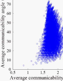
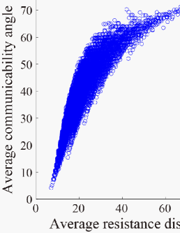
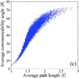
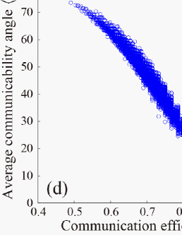
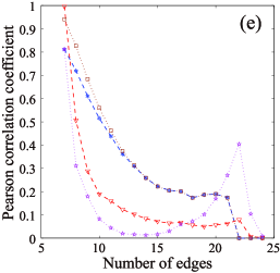
Fig. 3: (a–d) Scatter plots of the average communicability angle against (a) the average communicability distance, (b) the average resistance distance, (c) the average path length and (d) the communication efficiency for all 11,117 connected graphs with 8 nodes. (e) The squared Pearson correlation coefficients between the metrics for 8-node graphs with a fixed number of edges. Red triangles connected by a broken line indicate the data from (a), pink stars connected by a dotted line indicate the data from (b), the blue stars connected by a broken line indicate the data from (c) and brown squares connected by a dotted line indicate the data from (d).

We can see that the communicability angle is not directly or trivially related to the other metrics. It is particularly interesting to see the lack of correlation between $\left\langle\theta\right\rangle$ and $\left\langle\xi\right\rangle$. They are highly uncorrelated although the two quantities are based on the same concept of communicability. This lack of correlation is not unexpected if we consider how the two measures and the communicability function are related to each other via Eq. (11). The average communicability angle shows more similar trends to the average path length $\left\langle l\right\rangle$, the average resistance distance $\left\langle\Omega\right\rangle$ and the communication efficiency $E$. The extreme values of these three measures coincide with those of $\left\langle\theta\right\rangle$, although there is a large dispersion in between. The general plots in Fig. 3 really hides the true lack of correlation that exists among these metrics and the communicability angle. To reveal more of these lack of correlations we plot the squared Pearson correlation coefficient between each metric and $\left\langle\theta\right\rangle$ for groups of graphs having the same number of edges. As can be seen in Fig. 3(e), as soon as the number of edges increases, the correlation between the pair of indices drops significantly. For instance, let us consider the communication efficiency, for which the correlation with $\left\langle\theta\right\rangle$ yields a correlation coefficient $r^{2}\approx 0.94$ for the 8-node trees. This correlation coefficient drops to $r^{2}\approx 0.31$ for graphs having 13 edges and to $r^{2}\approx 0.17$ for graphs having 18 edges. It is virtually zero for graphs with more than 22 edges. The reason for this decay in the correlation is very important. Trees have very large correlations between the pairs of measures. This is due to the fact that in these graphs there are only shortest paths to connect any pair of nodes because of the absence of any cycles. As the number of edges increases the number of potential routes between any pair of nodes increases dramatically, making more different the measures based on shortest paths from the communicability angle. There is also a complete lack of correlation between the communicability angle and the average resistance distance for graphs having 10 to 20 nodes. The correlation coefficient increases for these two measures when the number of edges is 23 but then decays. The reason for this increase is not clear at all, but in any case the correlation coefficient indicates that the variance in one of the indices explained by the other is only 40% at this point.

Among all the connected graphs with 8 nodes, the path graph $P_{8}$ has the largest average communicability angle and the complete graph $K_{8}$ has the smallest. Among all the trees with 8 nodes, the star graph $K_{1,7}$ has the smallest average communicability angle. This is also verified for all connected graphs with 5, 6 and 7 nodes. We thereby have the following:

Conjecture 6.10.

Among all connected graphs with $n$ nodes, the average communicability angle is the largest for the path graph $P_{n}$ and the smallest for the complete graph $K_{n}$.

Conjecture 6.11.

Among all trees with $n$ nodes, the average communicability angle is the largest for the path graph $P_{n}$ and the smallest for the star graph $K_{1,n-1}$.

These observations indicate that the average communicability angle describes the efficiency of a graph in using the space in which it is embedded. The path graph $P_{n}$, which intuitively occupies the largest portion of space, has the largest average communicability angle, while the star and complete graphs, which intuitively occupy the smallest, have the average communicability angle close to zero. In the next section we explore more observations of this sort from a computational point of view.

6.2 Communicability angle and graph planarity

Here we investigate the relation between the graph planarity and the average communicability angle. We first determine whether a graph is planar or not using the planarity test proposed by Boyer and Myrvold [6]. We then construct the histogram of the frequency of planar/nonplanar graphs with respect to the average communicability angle.

Let $\eta_{k}$ be the number of planar graphs having $k\leq\left\langle\theta\right\rangle<\left(k+10^{\circ}\right)$ for $k=0^{\circ},10^{\circ},20^{\circ},\cdots,80^{\circ}$. We plot in Fig. 4(a) the histogram of the planar/nonplanar graphs as a function of their values of $\left\langle\theta\right\rangle$ for all connected graphs with 8 nodes.

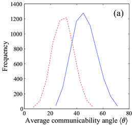
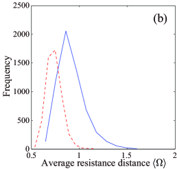
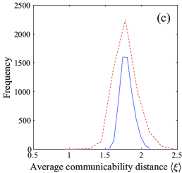
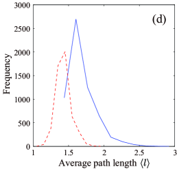
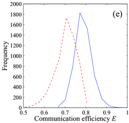
Fig. 4: Frequency of planar and nonplanar graphs for different values of (a) the average communicability angle, (b) the average resistance distance, (c) the average communicability distance, (d) the average path length, and (e) the communication efficiency. The histogram for planar graphs is shown as a solid line and that for nonplanar graphs as a broken line.

For comparison, we also show similar plots in Fig. 4(b–d) for the average resistance distance $\left\langle\Omega\right\rangle$, the communicability distance $\left\langle\xi\right\rangle$ and the average path length $\left\langle l\right\rangle$.

The first interesting observation is that the planar graphs yield significantly larger values of $\left\langle\theta\right\rangle$ than the nonplanar graphs. The peaks in the histogram Fig. 4(a) for the planar and nonplanar graphs are at $\left\langle\theta\right\rangle\approx 44.87^{\circ}$ and $\left\langle\theta\right\rangle\approx 32.17^{\circ}$, respectively. There is a larger relative separation between the two peaks of the histogram for $\left\langle\theta\right\rangle$ than for the rest of the measures. Let us put this in a quantitative context. Let us define the percentage of variation between the maxima of the two peaks as: $v\left(\%\right)=100\times\left(x_{h}\left(\mathrm{planar}\right)-x_{h}\left(\mathrm{nonplanar}\right)\right)/\left(x_{\mathrm{max}}-x_{\mathrm{min}}\right)$, where $x_{h}\left(\cdots\right)$ is the value of the corresponding variable for the peak in the histogram, while and $x_{\mathrm{max}}$ and $x_{\mathrm{min}}$ are the maximum and minimum values, respectively, of this variable $x$ for the whole dataset of 8-node graphs. For instance, for $x=\left\langle\theta\right\rangle$, the values are $x_{h}\left(\mathrm{planar}\right)=44.87^{\circ}$, $x_{h}\left(\mathrm{nonplanar}\right)=32.17^{\circ}$, $x_{\mathrm{max}}=73.55^{\circ}$ and $x_{\mathrm{min}}=4.19^{\circ}$. Then, the percentages of the variation between the maxima of the two peaks are: $18.3\%$ for $\left\langle\theta\right\rangle$, $13.4\%$ for $E$, $9.7\%$ for $\left\langle\Omega\right\rangle$, and $7.7\%$ for $\left\langle l\right\rangle$. As it is obvious from Fig. 4(c) this percentage is zero for the communicability distance. We have repeated these experiments by considering all the 261,080 connected graphs with 9 nodes, and the results are as follow: $23.2\%$ for $\left\langle\theta\right\rangle$, $15.3\%$ for $E$, $10.7\%$ for $\left\langle\Omega\right\rangle$, and $9.4\%$ for $\left\langle l\right\rangle$. Thus, it is clear that the communicability angle not only shows the best separation between planar and nonplanar graphs but also has the largest increase in this separation when increasing the number of nodes.

We can elaborate more on the relation between planarity and the communicability angle from the analysis of the connected graphs with 8 nodes: (i) No planar graph has $\left\langle\theta\right\rangle<21.4^{\circ}$; (ii) The planar graphs with the smallest value of $\left\langle\theta\right\rangle$ correspond to the maximal planar graphs. A graph is maximal planar, also known as a triangulation, if the addition of any edge to it results in a nonplanar graph. Obviously, these are the ‘least planar’ of all planar graphs. Examples are given in Fig. 5;

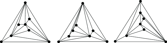
Fig. 5: Three maximal planar graphs with 8 nodes which have the smallest values of $\left\langle\theta\right\rangle$. The graphs are drawn as triangulations using Schnyder embedding [41]. Because the graphs are maximal planar, adding any edge will make the resulting graph nonplanar.

(iii) There is no nonplanar graph with $\left\langle\theta\right\rangle>55.065^{\circ}$; (iv) The nonplanar graphs with the largest values of $\left\langle\theta\right\rangle$ are minimal nonplanar graphs. A minimal nonplanar graph is a nonplanar graph for which every proper subgraph is planar, i.e., removing any node or edge makes the graph planar. Again, these are the ‘least nonplanar’ of all the nonplanar graphs. Examples are given in Fig. 6.

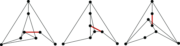
Fig. 6: Three minimal nonplanar graphs with 8 nodes which have the largest values of $\left\langle\theta\right\rangle$. The graphs are drawn using the Schnyder embedding [41] and allowing the superposition of one edge (marked in red thick line), whose removal will transform the graph into a planar one.

The previous results do not necessarily mean that the average communicability angle characterizes the graph planarity or vice versa, but that the planarity is indeed an important ingredient of the communication efficiency as measured by the communicability angle.

6.3 Communicability angle and graph modularity

Modularity is a very important concept for the study of real-world networks. It refers to the property of graphs with clusters of highly interconnected nodes but with poor inter-cluster connectivity. Such clusters are usually referred to as communities in network theory and are expected to play fundamental organizational roles in real-world networks, e.g., groups of proteins with similar actions and groups of people with common interests.

As a first example we construct random modular graphs in the following way. We generate random modular graphs with 1000 nodes and 50 modules. Then, with a fixed total edges density we systematically increases the proportion of edges within modules compared to edges across modules. As this proportion of intra-modular edges to inter-modular edges increases, the graphs become more modular in the sense previously explained. In order to capture the degree of modularity of these graphs we use the Newman modularity index [37], which is defined as

(34) $$Q=\sum_{k=1}^{n_{C}}\left[\dfrac{E_{k}}{m}-\dfrac{1}{4m^{2}}\left(\sum_{j\in V_{k}}k_{j}\right)^{2}\right],$$

where $E_{k}$ is the number of edges in the $k$th module, $n_{C}$ is the total number of modules, $m$ the total number of edges and $k_{j}$ the node degree.

In Fig. 7 we illustrate the results of plotting the modularity of the random modular graphs and the average communicability angle. As can be seen, as the modularity tends to its maximum, the average communicability angle tends to $90^{\circ}$, indicating the decrease in the spatial efficiency of these graphs.

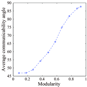
Fig. 7: Relation between the Newman modularity index [37] and the average communicability angle for random modular graphs with 1000 nodes and 50 modules. The total edge density is 0.01 and the proportion of intra- to inter-modular edges varies from 0.1 to 0.95. The points in the plot indicate the average of 100 random realizations. The broken line is to guide the eye.

A network with such clusters has structural bottlenecks; that is, if small groups of nodes/edges are removed the network is disconnected into two or more relatively large connected components. An extreme case are the dumbbell graphs $K_{n}$-$K_{n}$, that is, two cliques of $n$ nodes connected by only one edge; the removal of the edge separates the network into two connected components of $n/2$ nodes each.

On the other hand, a super-homogeneous graph, which is usually referred to as a good expansion graph, is characterized by the fact that every subset $S$ with more than $n/2$ nodes has a large boundary, which is the number of edges with one node inside the set $S$ and the other in $\overline{S}$ [39]. Expander graphs are characterized by having a large spectral gap $\lambda_{1}-\lambda_{2}$ of the adjacency matrix [2]; see Refs. [27, 32] for details.

What is important for the present subsection is that expanders are characterized by the lack of modularity, i.e., the lack of tightly connected clusters which are poorly interconnected by structural bottlenecks. In networks where $\lambda_{1}\gg\lambda_{2}$, we have the following expression for the communicability angle:

(35) $$\cos\theta_{pq}=\dfrac{G_{pq}}{\sqrt{G_{pp}G_{qq}}}\simeq\dfrac{\psi_{1}\left(p\right)\psi_{1}\left(q\right)e^{\lambda_{1}}}{\sqrt{\psi_{1}\left(p\right)^{2}e^{\lambda_{1}}\psi_{1}\left(q\right)^{2}e^{\lambda_{1}}}}=\cos 0^{\circ}.$$

That is, the networks lacking any modularity are characterized by very small value of the communicability angle. On the other hand, in a network where $\lambda_{1}$ is not significantly larger than $\lambda_{2}$, we make use of the expansions

$$G_{pp}G_{qq} =\psi_{1}(p)^{2}\psi_{1}(q)^{2}e^{2\lambda_{1}}+\left(\psi_{1}(p)^{2}\psi_{2}(q)^{2}+\psi_{2}(p)^{2}\psi_{1}(q)^{2}\right)e^{\lambda_{1}+\lambda_{2}}$$

(36) $$+\psi_{2}(p)^{2}\psi_{2}(q)^{2}e^{2\lambda_{2}}+\mathrm{h.o.},$$

$${G_{pq}}^{2} \simeq\psi_{1}(p)^{2}\psi_{1}(q)^{2}e^{2\lambda_{1}}+2\psi_{1}(p)\psi_{1}(q)\psi_{2}(p)\psi_{2}(q)e^{\lambda_{1}+\lambda_{2}}$$

(37) $$+\psi_{2}(p)^{2}\psi_{2}(q)^{2}e^{2\lambda_{2}}+\mathrm{h.o.},$$

where h.o. denotes the higher-order terms. The communicability angle is thereby transformed into the form

(38) $$\cos\theta_{pq}=\dfrac{G_{pq}}{\sqrt{{G_{pq}}^{2}+\left(\psi_{1}(p)\psi_{2}(q)-\psi_{2}(p)\psi_{1}(q)\right)^{2}e^{\lambda_{1}+\lambda_{2}}+\mathrm{h.o.}}}.$$

The second term in the denominator depends on the size of the spectral gap; the closer $\lambda_{2}$ is to $\lambda_{1}$, i.e., the smaller the spectral gap, the larger the denominator is, and consequently, the smaller Eq. (38) is. Therefore, the angle $\theta_{pq}$ is larger as the spectral gap is smaller. We should remark here that $\theta_{pq}$ does not depend only on the spectral gap because the higher-order terms in Eq. (38) can make an important contribution.

Let us show examples that illustrate the above important relation between the communicability angle and the graph modularity. Here again we focus on $\left\langle\theta\right\rangle$. We first consider the dumbbell graph $K_{3}$-$K_{3}$ shown in Fig. 8(a).

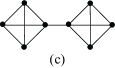
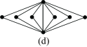
Fig. 8: The graphs with 6 nodes and 7 edges (a) with the largest and (b) the smallest average communicability angles. The same for the graphs with 8 nodes and 13 edges (c) and (d).

It consists of two cliques of 3 nodes each, which are connected by a link, thus having 7 edges in total. The average communicability angle for this graph is $\left\langle\theta\right\rangle\approx 57.105$ and its spectral gap is $\Delta\approx 0.682$. Among the 19 graphs with 6 nodes and 7 edges, the dumbbell $K_{3}$-$K_{3}$ has the largest value of $\left\langle\theta\right\rangle$. The smallest value of the average communicability angle is obtained for the graph in Fig. 8(b), having $\left\langle\theta\right\rangle\approx 47.935$ and $\Delta\approx 2.284$.

The situation is very similar for the 1,454 graphs with 8 nodes and 13 edges, among which the dumbbell graph $K_{4}$-$K_{4}$ in Fig. 8(c) has the largest average communicability angle $\left\langle\theta\right\rangle\approx 53.876$ with the spectral gap $\Delta\approx 0.511$. The graph with the smallest value of $\left\langle\theta\right\rangle$ is the so-called agave graph shown in Fig. 8(d); it consists of two connected nodes each of which is also connected to the other $n-2$ nodes that are not connected among them. It has $\Delta=4.00$ and $\left\langle\theta\right\rangle\approx 31.782$. The graphs with the second and third smallest average communicability angles, $\left\langle\theta\right\rangle\approx 35.123$ and $\left\langle\theta\right\rangle\approx 35.606$ with $\Delta\approx 2.988$ and $\Delta\approx 3.337$, respectively, have structures similar to the agave graph. Notice that the agave graph can be disconnected by removing two edges, but the remaining principal connected component has $n-1$ nodes, while the removal of 50% of the edges in this graph creates a principal connected component still containing 62.5% of the nodes. This shows the robustness of this graph to edge removal, a characteristic of good expander graphs due to the lack of structural bottleneck.

Figure 9(a–b) shows planar embeddings of the graphs in Fig. 8(a–b), respectively, onto triangular lattices.

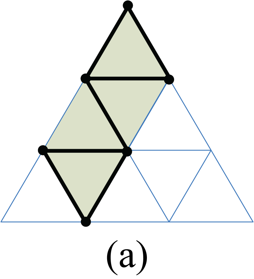
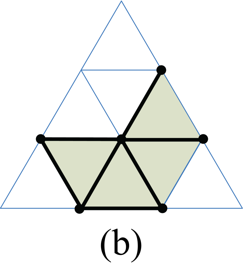
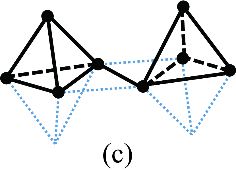
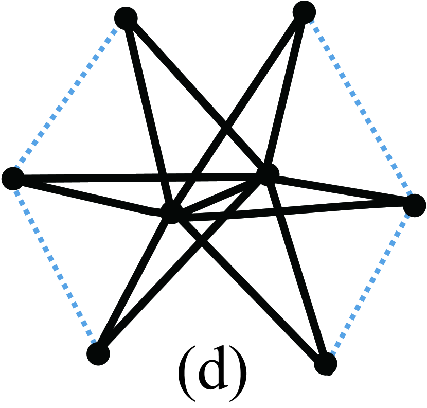
Fig. 9: (a–b) Planar embeddings of the graphs in Fig. 8(a–b), respectively, onto triangular lattices. (c–d) Three-dimensional embeddings of the graphs in Fig. 8(c–d), respectively, onto close-packed lattices.

The shadowed areas indicate the triangles covered by the graphs in these embeddings. Although both cover the four triangles, the latter graph, the one with the smallest average communicability angle, covers the most efficient packing in two-dimensional space, which is the area with a node surrounded by six others forming a hexagon. This is known as the penny-packing problem; see Ref. [24] for further information. The embedding of the graph with higher modularity and the largest average communicability angle is far from this optimal configuration.

A similar situation occurs with the graphs in Fig. 8(c–d), the ones with the largest and smallest $\left\langle\theta\right\rangle$ among those with 8 nodes and 13 edges; Fig. 9(c–d) show their embeddings onto close-packed lattices. We can conclude from these observations that a large average communicability angle indicates a poor spatial efficiency of the graph, while a small value of $\left\langle\theta\right\rangle$ is associated to the efficient use of space.

6.4 Communicability angle and graph holes

Another characteristic of spatial efficiency that is desirable to be captured by the average communicability angle is the existence of holes. The presence of large holes in a graph obviously makes its spatial efficiency very poor. For instance, let us consider a city in which all the street form annulus such that the whole center of the city is empty. The density of streets in that city is very small in comparison to what it is expected from the area occupied by the whole city.

Here we propose to consider the Sierpinski graphs as a model of simple graphs embedded in a Euclidean space such that the density of the graphs decays with the size. By the density we mean here the number of nodes divided by the area occupied by the corresponding external triangle. Let us denote by

(39) $$\vec{e}_{1}=\left(1,0,0\right),\>\vec{e}_{2}=\left(0,1,0\right),\>\vec{e}_{3}=\left(0,0,1\right)$$

the canonical basis vectors of $\mathbb{R}^{3}$. The Sierpinski graphs are generated iteratively from $G_{0}=\left(V_{0},E_{0}\right)$, where $V_{0}=\left\{\vec{e}_{1},\vec{e}_{2},\vec{e}_{3}\right\}$ and $E_{0}=\left\{\left(\vec{e}_{1},\vec{e}_{2}\right),\left(\vec{e}_{2},\vec{e}_{3}\right),\left(\vec{e}_{3},\vec{e}_{1}\right)\right\}$. Then, for $G_{k}=\left(V_{k},E_{k}\right)$ we have [42]

(40) $$V_{k>0} =\left(2^{k-1}\vec{e}_{1}+V_{k-1}\right)\cup\left(2^{k-1}\vec{e}_{2}+V_{k-1}\right)\cup\left(2^{k-1}\vec{e}_{3}+V_{k-1}\right),$$

(41) $$E_{k>0} =\left(2^{k-1}\vec{e}_{1}+E_{k-1}\right)\uplus\left(2^{k-1}\vec{e}_{2}+E_{k-1}\right)\uplus\left(2^{k-1}\vec{e}_{3}+E_{k-1}\right),$$

where $\uplus$ represents the disjoint union of sets. We illustrate in Fig. 10 the Sierpinski graphs $G_{1}$, $G_{2}$ and $G_{3}$. The total area occupied by the graph is the area of the external triangle which have coordinates $\left(2k,0,0\right),\left(0,2k,0\right),\left(0,0,2k\right)$. Notice that the Sierpinski graphs $G_{0}$ and $G_{1}$ do not have any holes, $G_{2}$ has a central hole of length 6 and $G_{3}$ has a central hole of length 12 plus 3 holes of length 6. As the graph grows, $G_{k}$ has the central hole of length $2^{k-1}\times 3$ with more holes of smaller sizes, and hence becomes more ‘spongy.’

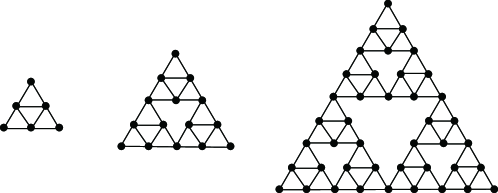
Fig. 10: The Sierpinski graphs $G_{1},$$G_{2}$ and $G_{3}$ (from left to right).

We have created the Sierpinski graphs for $k=1,\cdots,7$ and calculated their densities defined as the number of nodes divided by the area of the external triangle. We illustrate in Fig. 11(a) the relation between the density of the Sierpinski graphs and the average communicability angle.

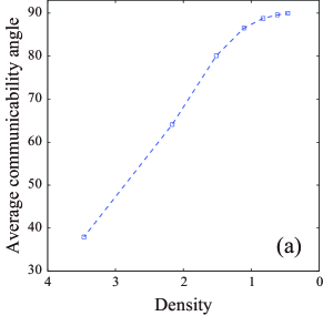
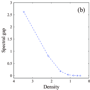
Fig. 11: Plots of (a) the variation of the average communicability angle and (b) the spectral gap of the adjacency matrix with the density of the Sierpinski graphs. The broken lines here are to guide the eye. Notice that the $x$ axis has a reverse scale.

For $G_{1}$, which contains no hole, the communicability angle is $\left\langle\theta\right\rangle\approx 37.96^{\circ}$ although the graph is planar. As the size of the graphs increases the average communicability angle quickly goes to its maximum for simple graphs, e.g. $\left\langle\theta\right\rangle\approx 90^{\circ}$ for $G_{7}$, which has 3,282 nodes. The results illustrated in Fig. 11(a) agrees with our intuition that the communicability angle accounts for the spatial efficiency of graphs. A Sierpinski graph with a large number of nodes, containing very large holes, e.g. the graph $G_{7}$ has a central hole of length 192, as well as many other holes of smaller sizes, lacks spatial efficiency in the sense of not using appropriately all the available space covered by the external triangles. In order to understand mathematically this relation we need to use the concept of isoperimetric number (4). We recall that a graph with a small isoperimetric number contains structural holes and/or bottlenecks, which are indications of poor spatial efficiency. Thus, we should expect that a large Sierpinski graph has a very small isoperimetric constant. Mohar [34] has found the following spectral bounds for the isoperimetric number of a graph:

(42) $$\dfrac{1}{2}\left(\delta-\lambda_{2}\right)\leq i\left(G\right)\leq\sqrt{\Delta^{2}-\lambda_{1}^{2}},$$

where $\delta$ and $\Delta$ are the minimum and maximum degree of the graph, respectively, and $\lambda_{j}$ are the eigenvalues of the adjacency matrix in a nonincreasing order as before. Consequently, for graphs with bounded maximum and minimum degree — such as the Sierpinski graphs, where $\delta=2$ and $\Delta=4$ — the isoperimetric number is determined by the spectral gap $\lambda_{1}-\lambda_{2}$. A large spectral gap indicates a large isoperimetric number, while a small spectral gap indicates a small isoperimetric number. We illustrate in Fig. 11(b) the plot of the density of the Sierpinski graphs against the spectral gap of their adjacency matrices. As can be seen, the Sierpinski graphs with small density, i.e., those with large number of nodes, have very small spectral gaps, and consequently small isoperimetric numbers.

On the contrary, if a graph has a large spectral gap, i.e., $\left(\lambda_{1}-\lambda_{2}\right)\rightarrow\infty$, the communicability function is given by

(43) $$G_{pq}\rightarrow\psi_{1,p}\psi_{1,q}\exp\left(\lambda_{1}\right),$$

which implies that

(44) $$\theta_{pq}\rightarrow 0^{\circ},\forall p,q\in V.$$

That is, a large isoperimetric number indicates that the graphs have a large spectral gap. At the same time, a large spectral graph indicates that the communicability angle is very small for every pair of nodes in the graph. As we have seen a small spectral gap, and consequently a small isoperimetric number, gives rise to a large communicability angle as in the case of large Sierpinski graphs. This conclusion again supports our idea that the communicability angle is a good indicator of the spatial efficiency of a given network.

6.5 Conclusions of the computational analysis of simple graphs

The main conclusion of Section 6 is the following: the average communicability angle very well describes a graph characteristic which represents their spatial efficiency. It is drawn from the following observations. First, planar graphs are not spatially efficient graphs; at the same time they have large average communicability angles. On the contrary, highly nonplanar graphs more efficiently use the available space; at the same time they have smaller values of $\left\langle\theta\right\rangle$. Second, a modular graph uses the available space less effectively than a nonmodular one; at the same time, modular graphs have relatively large values of the average communicability angle. Third, graphs containing structural holes, which are not spatially efficient, display large communicability angles, while those having large isoperimetric numbers and consequently good spatial efficiency have communicability angles close to zero.

We should, however, be careful in analyzing more complex situations in which combinations of properties, such as nonplanarity and modularity, or nonplanarity and structural hole, are present. In general, we consider that graphs with relatively small values of the average communicability angle exhibit higher spatial efficiency than those with relatively larger values.

7 Communicability angle in real-world networks

We start this section by considering the average communicability angle of a series of 120 complex networks arising from various scenarios. The networks are briefly described in Supplementary Information accompanying this paper, where references to the original datasets are provided. The series includes networks in which the nodes and links are clearly embedded into geometrical spaces, such as urban street networks, networks formed by animal nests, brain and neural networks, protein-residue networks as well as electronic circuits and the Internet. It also includes networks in which the nodes and links can hardly be allocated to geographic positions, such as food webs, social networks and software networks. The biomolecular networks including protein-protein interaction and gene transcription networks are also non-geographically embedded ones.

7.1 Global properties of the communicability angle

The 120 real-world networks studied here cover the whole spectrum of values of the average communicability angle from $\left\langle\theta\right\rangle\approx 10^{-5}{}^{\circ}$ for the food web of Shelf to $\left\langle\theta\right\rangle\approx 89.9^{\circ}$ for the Power Grid network of western USA.

The average communicability angle of these real-world networks is not correlated to the average path length, the communication efficiency or the resistance distance (see Supplementary Information accompanying this paper). Just to mention an example, let us consider the network of galleries created by ants and the collaboration network associated with Linux open-source software system (see Supplementary Information for details). The first network is planar due to the fact that ants are obliged to create their corridors and galleries in a very thin layer of sand. The second one is a highly nonplanar network. Both networks have the communication efficiency $E\approx 0.24$; according to this index the two graphs are equally efficient in transmitting information, something hard to believe taking into account their different topologies and functionalities. The average communicability angle, on the other hand, clearly indicates the fact that the software network is highly efficient $\left\langle\theta\right\rangle\approx 3.47^{\circ}$ while the ant network is very inefficient $\left\langle\theta\right\rangle\approx 85.51^{\circ}$. There are many more examples that can be extracted from the information provided in the Supplementary Information accompanying this paper, all of which point to the fact that the average communicability angle is a good index to account for communication and spatial efficiency of networks.

The histogram in Fig. 12 shows two prominent peaks at $0^{\circ}\leq\left\langle\theta\right\rangle\leq 9^{\circ}$ and at $81^{\circ}\leq\left\langle\theta\right\rangle\leq 90^{\circ}$.

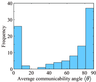
Fig. 12: Histograms of the average communicability angle in 120 real-world networks with the bin size of $9^{\circ}$.

A more detailed view (not shown) indicates that the highest frequency occurs at $0^{\circ}\leq\left\langle\theta\right\rangle\leq 1^{\circ}$, followed by the one at $89^{\circ}\leq\left\langle\theta\right\rangle\leq 90^{\circ}$. That is, the real-world networks are very much polarized into the two extremes; either they have very small values of the communicability angle or very large ones.

Certain classes of networks have a large homogeneity in the values of the average communicability angle. The 1997 and 1998 versions of the Internet at Autonomous System (AS) have the average communicability angles of $0.78^{\circ}$ and $0.42^{\circ}$, respectively. There is also a large homogeneity among the brain/neural networks, namely, the visual-cortex networks of cat and macaque as well as the neural network of C. elegans, which have $\langle\!\langle\theta\rangle\!\rangle=1.77^{\circ}\pm 1.66^{\circ}$, where the double brackets $\langle\!\langle\cdots\rangle\!\rangle$ denote the average value of the average communicability angles for a series of networks. In addition, the classes of urban street networks formed by 14 networks and the one of protein-residue networks formed by 40 networks also show remarkable homogeneity. For instance, the urban street networks have $\langle\!\langle\theta\rangle\!\rangle=86.07^{\circ}\pm 5.07^{\circ}$ and the protein-residue networks have $\langle\!\langle\theta\rangle\!\rangle=78.83^{\circ}\pm 7.28^{\circ}$. The ranking of the 14 cities in the former is: Barcelona $<$ Rio Grande $<$ Yuliang $<$ Chegkan $<$ Atlanta $<$ Berlin $<$ Rotterdam $<$ Hong Kong $<$ Mecca $<$ Cambridge $<$ Oxford $<$ Ahmedabad $<$ Milton Keynes. This means that in terms of the effective communication among the different regions of the city, Barcelona is the most effective one, while Milton Keynes the worse.

The homogeneity among the protein-residue networks is more unexpected than that among the urban street networks because they represent three-dimensional (3D) objects. Proteins are folded into 3D structures forming topologies consisting of a mix of $\alpha$-helices and $\beta$-sheets. They also have different shapes and sphericities. It is therefore surprising that the protein-residue networks are characterized by very large values of the communicability angle, which are more characteristic of planar or almost planar networks, as demonstrated for the urban street networks.

Although we will go back below to the relation between the communicability angle and the structure of proteins, let us make a comment here. The fact that proteins are embedded into the 3D physical space does not necessarily mean that their residue networks are nonplanar. The same applies to other naturally evolving networks, such as the networks of galleries and corridors formed by termite mounds, which are also characterized by very large average communicability angles with $\langle\!\langle\theta\rangle\!\rangle=88.33^{\circ}\pm 1.01^{\circ}$. Although the mounds are constructed in the 3D space, they are remarkably close to planar graphs; we have indeed found that by removing only 6% of the edges of these networks the graphs representing them become planar. Both the termite mounds and the protein-residue networks have certainly evolved in the 3D space, but the networks must be close to planar graphs for different ecological or biological reasons. In the termite mounds the use of a large volume of the 3D space is needed to produce a ventilation system necessary to discharge the carbon dioxide produced in its interior. For protein, structures close to planar ones are needed to avoid high compactness that destroy the internal cavities of the protein needed for developing their functions; see Section 7.2 below.

On the other hand, the values of $\left\langle\theta\right\rangle$ obtained for the software networks [35] are unexpectedly heterogeneous. These networks yield $\langle\!\langle\theta\rangle\!\rangle=57.6^{\circ}\pm 30.7^{\circ}$ with the values ranging from $\left\langle\theta\right\rangle\approx 3.465^{\circ}$ for Linux to $\left\langle\theta\right\rangle\approx 84.323^{\circ}$ for XMMS. The ranking of these networks in terms of the average communicability angle is: Linux $<$ MySQL $<$ VTK $<$ Abi Word $<$ Digital Material $<$ XMMS. The classes of social and biological networks consisting of 14 and 11 networks, respectively, also show relatively large variability in their values of the communicability angle: $\langle\!\langle\theta\rangle\!\rangle=55.8^{\circ}\pm 21.3^{\circ}$, and $\langle\!\langle\theta\rangle\!\rangle=63.3^{\circ}\pm 17.0^{\circ}$, respectively. This is not surprising; we can easily associate it to the diversity of networks in these classes.

What is really surprising is that the food webs, which form a very homogeneous class of networks in terms of the relations accounted for them, yield a relatively large standard deviation in the values of the communicability angle: $\langle\!\langle\theta\rangle\!\rangle=7.1^{\circ}\pm 16.1^{\circ}$ with the values ranging from $\left\langle\theta\right\rangle\approx 10^{-5}{}^{\circ}$ for the marine system of Shelf to $\left\langle\theta\right\rangle\approx 78.356^{\circ}$ for the web of the English grassland. The ranking of these food webs in terms of the average communicability angle is: Shelf $<$ Elverde $<$ Skipwith $<$ ReefSmall $<$ LittleRock $<$ Stony $<$ Coachella $<$ Canton $<$ Benguela $<$ BridgeBrook $<$ Ythan2 $<$ Ythan1 $<$ StMartins $<$ StMarks $<$ ScotchBroom $<$ Chesapeake $<$ Grassland.

In terms of the individual values of $\left\langle\theta\right\rangle$, the results obtained for these 120 networks agree with our findings in the previous section. The largest average communicability angles are observed for the Power Grid of western USA and urban street networks, which are planar or almost planar with both nodes and edges embedded into a plane. On the other extreme of the smallest average communicability angles, there are networks which are highly nonplanar, such as the USA air transportation network, a world trade network, the Internet at AS, and brain/neural networks. All these networks have nodes embedded into two- or three-dimensional spaces, such as cities, countries or organs, but the edges connecting them very efficiently use the available space. We would like to remark here that the small values of $\left\langle\theta\right\rangle$ observed in some classes of networks do not necessarily mean a high interconnection density. For instance, the USA airport transportation network and the two versions of the Internet studied here have relatively small edge densities: 0.039 and 0.0011, respectively.

7.2 Communicability angle and spatial efficiency of proteins

We have accumulated several pieces of empirical evidence that support the idea that the average communicability angle accounts for the spatial efficiency of graphs. It is, however, generally difficult to find quantitative measures of the spatial efficiency in real-world complex networks to compare with the communicability angle.

An exception to this is provided by proteins, which are 3D objects characterized by different degrees of packing or spatial efficiency. In this section we study the relation between the average communicability angle and the spatial efficiency of the protein-residue networks for a group of 40 proteins whose 3D structures have been resolved by X-ray crystallography and deposited in the protein databank (PDB) [5]. Here each node represents an amino acid in the protein and two nodes are connected if the corresponding amino acids are separated at a distance of no more than 7Å in the 3D structure of the protein as determined experimentally [3].

A protein is a linear sequence of amino acids connected by peptide bonds. The chain is folded into a 3D shape unique to each protein. While the amino-acid sequence forms the so-called primary structure of the protein, the 3D folding defines its secondary and tertiary structures. The secondary one is characterized by the presence of the $\alpha$-helices and the $\beta$-sheets, while the tertiary one is formed by global positioning of the secondary one into a 3D shape that gives the protein its globular-like structure [10]. The folding of the proteins is the consequence, grosso modo, of two main necessities that the protein has: (i) protecting the hydrophobic amino acids from their contact with water; (ii) occupying a minimum space inside the limited volume of the cell. Thus the packing of a protein is related to its spatial efficiency [21], which is responsible for many of its physico-chemical and biological properties.

There are many ways of quantifying the packing of a protein, but here we consider the following one. Let $V_{e}$ be the volume of a protein which is expected from its ideal 3D structure and let $V_{o}$ be the volume which is actually observed in its X-ray crystallography. We then define the relative deviation from its ideal volume as

(45) $$P=\dfrac{V_{e}-V_{o}}{V_{e}}.$$

Hereafter we call $P$ the relative packing efficiency of the protein. A positive value of $P$ means that the protein is more packed than expected from its ideal 3D structure, that it is highly efficient in using the 3D space, at least relatively to the ideal structure. A negative value of $P$, on the other hand, means that it is less packed than expected, that it is not spatially efficient. We should mention here that values that deviate very much from the expected or ideal values can indicate possible problems with the structure and as such should be discarded from the analysis.

Using computational techniques and VADAR software described in Ref. [43], we have calculated the expected and observed volumes of the 40 proteins. We show in Fig. 13 the relation between the relative packing efficiency $P$ and the average communicability angle of the 40 proteins.

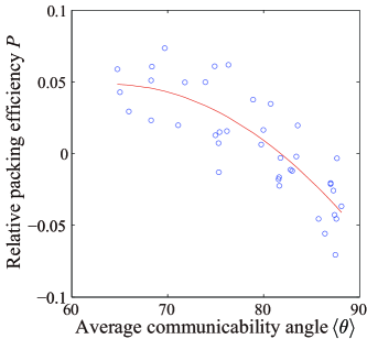
Fig. 13: Linear correlation between the average communicability angle of proteins represented by residue networks and the relative packing efficiency.

The Pearson correlation coefficient is $R=-0.837$, indicating a significant correlation between the two variables. We can summarize the results as follows: (i) proteins with poor spatial efficiency, $P<0$, have $\left\langle\theta\right\rangle>81^{\circ}$; (ii) those with high spatial efficiency, $P>0$, have $\left\langle\theta\right\rangle<80^{\circ}$. In other words, small average communicability angles are related to high spatial efficiency of proteins while large average communicability angles with a poor use of space. We notice in passing that there are no proteins with $\left\langle\theta\right\rangle<60^{\circ}$, which can be explained by the fact that increasing too much packing would make the internal cavities of the protein disappear [21]. The internal cavities are responsible for the interaction of proteins with other biological molecules and usually play a fundamental role in their functionality. In general, we can conclude that proteins are spongy in a similar way as the Sierpinski graphs are.

Possibilities which the communicability angle brings to the analyses of the structure of spatially embedded complex networks obviously go beyond the use of $\left\langle\theta\right\rangle$. For instance, the contour plot of the communicability angle for every pair of residues in a protein can reveal important properties of its 3D structure. Figure 14 shows an example of the protein with PDB code 1amm, which corresponds to the GammaB crystalline, whose crystallographic analysis was carried out at 150K.

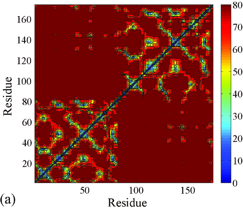
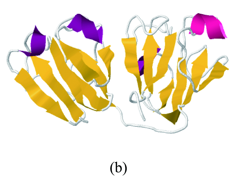
Fig. 14: (a) Contour plot of the communicability angle between every pair of residues in the GammaB crystalline protein with PDB code 1amm. (b) A cartoon representation of the protein with PDB code 1amm in which the $\beta$-sheets are represented as arrows in yellow and the helices as ribbons in magenta. This shows the existence of two domains in it.

This protein consists of two $\alpha,\beta$-domains, the first of which formed by amino acids 1-83 and the second by amino acids 84-174. The two domains are very well reflected in the contour plot Fig. 14(a) as two main diagonal blocks of relatively small communicability angles, which indicates good internal communication in each domain.

7.3 Spatial efficiency in networks under external stress

The communicability function has been previously generalized to consider an external stress to which the network is submitted. This external stress is accounted for by means of the so-called inverse temperature $\beta\equiv\left(k_{B}T\right)^{-1}$, where $k_{B}$ is a constant and $T$ is the temperature [15]. This analogy results from regarding that the whole network is submerged into a thermal bath of the inverse temperature $\beta$; see [17, 11] for details. After equilibration in the bath, all edges of the network acquire a weight equal to $\beta$.

It is clear that when $\beta\rightarrow 0$, i.e., as the temperature tends to infinite, the network becomes disconnected and there is no communication among any pair of nodes. This resembles a gas in which every node is an independent particle. On the other hand, when $\beta\rightarrow\infty$, i.e., the temperature tends to zero, the weights of every edge becomes extremely large, which definitively increases the communication capacity among the pairs of connected nodes. The temperature thus plays a role of an empirical parameter which is useful in simulating effects of external stresses to which the network is submitted, such as different levels of social agitation, economical situations, environmental stress, variable physiological conditions, etc. Under this analogy, we generalized the communicability function (2) into the form [15]

(46) $$G_{pq}\left(\beta\right)=\left(e^{\beta A}\right)_{pq}.$$

It is straightforward to realize that the communicability angle between a given pair of nodes is generalized to

(47) $$\cos\theta_{pq}\left(\beta\right) =\frac{G_{pq}\left(\beta\right)}{\sqrt{G_{pp}\left(\beta\right)G_{qq}\left(\beta\right)}}.$$

Let us conduct a simple experiment to explore the possibilities which this empirical parameter brings to the analysis of real-world scenarios. We use two urban street networks representing the city landscapes of Rio Grande in Brazil and of Yuliang in China. Both cities have large values of the average communicability angle, i.e., small spatial efficiency, with $\left\langle\theta\right\rangle\approx 79.7^{\circ}$ and $\left\langle\theta\right\rangle\approx 85.8^{\circ}$, respectively. We then lower the temperature and see if it increases the spatial efficiency of both cities, i.e., if it decreases the values of $\left\langle\theta\right\rangle$. In other words, we systematically increase $\beta$ and compute the average communicability angle $\langle\theta(\beta)\rangle$. The increase in $\beta$ here can be associated to the average increment in the number of lanes per street in the city.

Figure 15(a) shows the results.

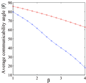
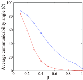
Fig. 15: (a) Effects of the inverse temperature $\beta$ on the average communicability angle in two urban street networks, Rio Grande, Brazil (blue squares) and Yuliang, China (red circles). (b) The same for two visual-cortex networks: cat (red circles) and macaque (blue squares).

The city of Rio Grande dramatically improves its spatial efficiency by increasing the average number of lanes of its streets. Although the improvement for Yuliang is not so dramatic, there is still a decrease in the average communicability angle of $20^{\circ}$. The causes for the difference in the variation of $\left\langle\theta\right\rangle$ with the temperature for different networks is not a trivial one, as there are likely to be many structural factors involved. We do not investigate these causes here.

We next carry out the opposite experiment using two brain networks representing the cat and macaque visual cortices. The average communicability angle shows that both networks have a great spatial efficiency: $\left\langle\theta\right\rangle\approx 0.22^{\circ}$ and $\left\langle\theta\right\rangle\approx 3.52^{\circ}$, respectively. We here raise the temperature, i.e., decrease $\beta$, and see if it deteriorates the connections in the visual cortices in terms of the average communicability angle $\langle\theta(\beta)\rangle$. The decrease of $\beta$ can be regarded as any malfunctioning or diseases.

Figure 15(b) shows the results. Both networks dramatically decrease their spatial efficiency as $\beta\rightarrow 0$; obviously, $\theta_{pq}\left(\beta=0\right)=90^{\circ}$. We notice, however, that the cat visual cortex is more resistant to the stress than the macaque one. For $\beta=0.6$, for example, the former has $\left\langle\theta\right\rangle\approx 3.15^{\circ}$ while the latter has jumped up to $\left\langle\theta\right\rangle\approx 29.9^{\circ}$.

The influence of the inverse temperature can be summarized as follows. In the limit $\beta\rightarrow\infty$, we have $G_{pq}\rightarrow\psi_{1,p}\psi_{1,q}\exp\left(\beta\lambda_{1}\right)$. This is equivalent to increase the good expansion properties of the network. We recall from previous sections that for expanders the spectral gap $\lambda_{1}-\lambda_{2}$ is very large, and consequently we have the above convergence. This is exactly the effect that we see; when we increase $\beta$, the networks become more spatially efficient, i.e., $\left\langle\theta\right\rangle\rightarrow 0^{\circ}$. In the limit $\beta\rightarrow 0$, on the other hand, we have $G_{pq}\rightarrow 1$, which implies that $\left\langle\theta\right\rangle\rightarrow 90^{\circ}$. This is equivalent to reducing dramatically the capacity of each edge of transmitting information in the network, which clearly decreases its communication and spatial efficiencies.

In closing, the use of the empirical parameter $\beta$ allows us to simulate the effects of external factors which can modify the spatial efficiency of a network. This brings a modeling scenario to assaying of strategies of improving the spatial efficiency of networks or to analyses of their resilience to external stresses.

8 Conclusions

In a network, the more abstract spatial efficiency refers to the average quality of communication among the nodes. Such communication goodness is quantified as the ratio of the amount of information successfully delivered to its destination to the one which is frustrated in its delivery and returned to its originators. This new paradigm is then mathematically formulated in terms of the communicability angle between a pair of nodes. We have provided analytical and empirical pieces of evidence which reaffirm the idea that the communicability angle accounts for the spatial efficiency of networks.

The richness of this approach goes beyond the results presented here; there are a few immediate directions of research in this area which can open new opportunities for the analysis of networks. The use of the communicability angle for a pair of connected nodes can be seen as an edge centrality measure which may reveal important characteristics of individual edges in networks. The communicability angle averaged over the edges incident to a given node can also represent a node centrality index which indicates the contribution of the node to the global spatial efficiency of a network. The study of the effects of the inverse temperature on the spatial efficiency and the determination of the most important structural factors that influence it is of tremendous practical importance. These studies will allow us not only to predict the effects of external stresses over the spatial efficiency of a network but also to assay theoretical scenarios of improving this efficiency in certain classes of networks. Last but not least, the new concept of communicability angle can bring new possibilities to the mathematical analysis of specific types of graphs and properties, such as planarity and graph thickness among others.

References

- [1] S. Achard and Ed Bullmore, Efficiency and cost of economical brain functional networks, PLoS Comput. Biol. 3 (2007) pp. e17.
- [2] N. Alon and V. D. Milman, , Isoperimetric inequalities for graphs, and superconcentrators, J. Combin. Theor. B, 38 (1985) pp. 73–88.
- [3] A. R. Atilgan, P. Akan, and C. Baysal, Small-world communication of residues and significance for protein dynamics, Biophys. J. 86 (2004) pp. 85–91.
- [4] M. Barthélemy, Spatial networks, Phys. Rep., 499 (2011) pp. 1–101.
- [5] H. M. Berman, J. Westbrook, Z. Feng, G. Gilliland, T. N. Bhat, H. Weissig, I. N. Shindyalov, and P. E. Bourne, The protein data bank, Nucleic Acids Res. 28 (2000) pp. 235–242.
- [6] J. M. Boyer and W. J. Myrvold, On the cutting edge: simplified planarity by edge addition, J. Graph Algorith. Appl. 8 (2004) pp. 241–273.
- [7] E. Bullmore and O. Sporns, Complex brain networks: graph theoretical analysis of structural and functional systems, Nature Rev. Neurosci., 10 (2009) pp. 186–198.
- [8] A. Cardillo, S. Scellato, V. Latora, and S. Porta, Structural properties of planar graphs of urban street patterns, Phys. Rev. E, 73 (2006) pp. 066107.
- [9] L. F. Costa, O. N. Oliveira Jr, G. Travieso, F. A. Rodrigues, P. R. Villas Boas, L. Antiqueira, M. P. Viana, and L. E. Correa Rocha, Analyzing and modeling real-world phenomena with complex networks: a survey of applications, Adv. Phys., 60 (2011) pp. 329–412.
- [10] E. Estrada, Characterization of the folding degree of proteins, Bioinformatics, 18 (2002) pp. 697–704.
- [11] E. Estrada, The Structure of Complex Networks. Theory and Applications, Oxford University Press, 2011.
- [12] E. Estrada, The communicability distance in graphs, Lin. Alg. Appl., 436 (2012) pp. 4317–4328.
- [13] E. Estrada, Complex networks in the Euclidean space of communicability distances, Phys. Rev. E, 85 (2012) pp. 066122.
- [14] E. Estrada, Graphs and Networks, in M. Grinfeld, ed. Mathematical Tools for Physicists, John Wiley & Sons, 2014.
- [15] E. Estrada and N. Hatano, Statistical-mechanical approach to subgraph centrality in complex networks, Chem. Phys. Lett., 439 (2007) pp. 247–251.
- [16] E. Estrada and N. Hatano, Communicability in complex networks, Phys. Rev. E, 77 (2008) pp. 036111.
- [17] E. Estrada, N. Hatano, and M. Benzi, The physics of communicability in complex networks, Phys. Rep., 514 (2012) pp. 89–119.
- [18] E. Estrada and D. J. Higham, Network properties revealed through matrix functions, SIAM Rev., 52 (2010) pp. 696–714.
- [19] E. Estrada and J.A. Rodríguez-Velázquez, Subgraph centrality in complex networks, Phys. Rev. E, 71 (2005) pp. 056103.
- [20] E. Estrada, M. G. Sanchez-Lirola, and J. A. de la Peña, Hyperspherical Embedding of Graphs and Networks in Communicability Spaces, Discr. Appl. Math., 176 (2014) pp. 53–77.
- [21] P. J. Fleming and F. M. Richards, Protein packing: dependence on protein size, secondary structure and amino acid composition, J. Mol. Biol. 299 (2000) pp. 487–498.
- [22] A. Ghosh, S. Boyd, and A. Saberi, Minimizing effective resistance of a graph, SIAM Rev., 50 (2008) pp. 37–66.
- [23] J. Goñi, A. Avena-Koenigsberger, N. V. de Mendizabal, M. van den Heuvel, R. Betzel and O. Sporns, Exploring the morphospace of communication efficiency in complex networks, PLoS One, 8 (2013) pp. e58070.
- [24] R. L. Graham and N. J. A. Sloane, Penny packing and two-dimensional codes, Discr. Comput. Geom., 5 (1990) pp. 1-11.
- [25] J. L. Gross and T. W. Tucker, Topological Graph Theory, Dover Pub., Inc., Mineola, N.Y., 1987.
- [26] J.L. Gross, J. Yellen, and P. Zhang, eds., Handbook of Graph Theory, CRC Press, Boca Raton, 2013.
- [27] S. Hoory, N. Linial, and A. Wigderson, Expander graphs and their applications, Bull. Am. Math. Soc., 43 (2006) pp. 439–561.
- [28] B. Jiang and C. Claramunt, Topological analysis of urban street networks, Environ. Plan. B, 31 (2004) pp. 151–162.
- [29] D. J. Klein and M. Randić, Resistance distance, J. Math. Chem., 12 (1993) pp. 81–95.
- [30] V. Latora and M. Marchiori, Efficient behavior of small-world networks, Phys. Rev. Lett. 87 (2001) pp. 198701.
- [31] V. Latora and M. Marchiori, Economic small-world behavior in weighted networks, Eur. Phys. J. B 32 (2003) pp. 249-263.
- [32] A. Lubotzky, Expander graphs in pure and applied mathematics, Bull. Am. Math. Soc., 49 (2012) pp. 113–162.
- [33] U. V. Luxburg, A. Radl, and M. Hein, Getting lost in space: Large sample analysis of the resistance distance, In Advances in Neural Information Processing Systems (2010) pp. 2622-2630.
- [34] B. Mohar, Isoperimetric inequalities, growth, and spectrum of graphs. Linear Algebra Appl., 103 (1983) pp. 119-131.
- [35] C. R. Myers, Software systems as complex networks: Structure, function, and evolvability of software collaboration graphs, Phys. Rev. E, 68 (2003) pp. 046116.
- [36] M. E. J. Newman, The structure and function of complex networks, SIAM Rev., 45 (2003) pp. 167–256.
- [37] M. E. J. Newman, Modularity and community structure in networks, Proc. Nat. Acad. Sci. 103 (2006) pp. 8577-8582.
- [38] D. Plavšić, S. Nikolić, N. Trinajstić, and Z. Mihalić, On the Harary index for the characterization of chemical graphs, J. Math. Chem. 12 (1993) pp. 235-250.
- [39] P. Sarnak, WHAT IS… an Expander?, Notices Am. Math. Soc., 51 (2004) pp. 762–763.
- [40] A. Sarzynski and A. Levy, Spatial Efficiency and Regional Prosperity: A Literature Review and Policy Discussion; prepared as background for GWIPP‘s — Implementing Regionalism project, funded by the Surdna Foundation. http://www.gwu.edu/~gwipp/SpatialEfficiencyWPAug16.pdf (downloaded on 20 November 2014).
- [41] W. Schnyder, Embedding planar graphs on the grid. In SoDA, 90 (1990) pp. 138-148.
- [42] E. Teufl, and S. Wagner, The number of spanning trees of finite sierpinski graphs. In Fourth Colloquium on Mathematics and Computer Science, volume AG of DMTCS Proceedings, pp. 411-414. 2006.
- [43] L. Willard, A. Ranjan, H. Zhang, H. Monzavi, R. F. Boyko, B. D. Sykes, and D. S. Wishart, VADAR: a web server for quantitative evaluation of protein structure quality, Nucleic Acids Res. 31 (2003) pp. 3316-3319.
- [44] W. Xiao and I. Gutman, Resistance distance and Laplacian spectrum, Theor. Chem. Acc., 110 (2003) pp. 284–289.
- [45] K. Xu and K. C. Das, On Harary index of graphs, Discr. Appl. Math. 159 (2011) pp. 1631-1640.
- [46] B. Zhou, X. Cai, and N. Trinajstić, On Harary index, J. Math. Chem. 44 (2008) 611-618.