Could the collision of CMEs in the heliosphere be super-elastic? — Validation through three-dimensional simulations
Abstract
Though coronal mass ejections (CMEs) are magnetized fully-ionized gases, a recent observational study of a CME collision event in 2008 November has suggested that their behavior in the heliosphere is like elastic balls, and their collision is probably super-elastic (C. Shen et al., 2012). If this is true, this finding has an obvious impact on the space weather forecasting because the direction and veliocity of CMEs may change. To verify it, we numerically study the event through three-dimensional MHD simulations. The nature of CMEs’ collision is examined by comparing two cases. In one case the two CMEs collide as observed, but in the other, they do not. Results show that the collision leads to extra kinetic energy gain by 3%–4% of the initial kinetic energy of the two CMEs. It firmly proves that the collision of CMEs could be super-elastic.
1 Introduction
Dynamic process of coronal mass ejections (CMEs) in the heliosphere is key information for us to evaluate the CMEs’ geo-effectiveness. But it becomes more complicated when successive CMEs interact in the heliosphere. Both observational and numerical studies have shown that CME’s shape, velocity and direction may change significantly through collisions and interactions (e.g., Wang et al., 2002, 2003, 2005; Reiner et al., 2003; Farrugia and Berdichevsky, 2004; Lugaz et al., 2005, 2009, 2012; Hayashi et al., 2006; Xiong et al., 2007; Wu et al., 2007; Liu et al., 2012; Temmer et al., 2012; Shen et al., 2012; C. Shen et al., 2012).
CMEs are magnetized plasmoids. In most cases, CMEs could be treated as an elastic ball in the heliosphere due to low reconnection rate, and the collision between them was usually thought to be elastic or inelastic, through which the total kinetic energy of colliding CMEs conserves or decreases. This classic collision picture was often used to analyze the momentum exchange during CME collisions (e.g., Lugaz et al., 2009; Temmer et al., 2012). But the picture is sometimes failed to explain observations. For example, the analysis of 2010 August 1 CME-CME interaction event suggested that the collision between CMEs is unlikely to be elastic or perfectly inelastic (Temmer et al., 2012). A possible explanation is that the CME-driven shock if any may be involved in the momentum transfer (Lugaz et al., 2009). Another explanation can be found in a most recent work about the CME-CME interaction event during November 2–8, 2008 by C. Shen et al. (2012), which for the first time revealed that the collision of CMEs could be super-elastic. A fundamental definition of super-elastic collision is that the total kinetic energy of colliding system increases after the collision. It is unexpectedly beyond the classic collision picture, but well explains the observed track of the leading CME in that event.
If super-elastic collision does happen, CME’s effect on space weather needs to be re-evaluated because more thermal and magnetic energy inside CMEs will be converted into kinetic energy, which may cause the changes of the direction and velocity of CMEs different from usually expected. However, at present, the finding of super-elastic is doubtable, because the result was obtained based on the remote imaging data from STEREO spacecraft and some highly ideal assumptions. Thus a numerical simulation may favor us validating the possibility of CMEs’ super-elastic collision.
In this letter, we carry out three-dimensional (3-D) MHD simulations based on the observations of the 2008 November event, and try to reveal the nature of the CMEs’ collision through the analysis of the energy transformation during the collision. In the next section, the MHD model and simulation method are introduced. The simulation results of the CMEs’ collision and a comparison with a non-collision case are presented in Section 3 and 4, respectively. In the last section, a summary and discussion is given.
2 MHD model and simulation method
The numerical scheme we used is a 3-D corona-interplanetary total variation diminishing (COIN-TVD) scheme in a Sun-centered spherical coordinate system (Feng et al., 2003, 2005; Shen et al., 2007, 2009). The projected characteristic boundary conditions (Wu and Wang, 1987; Hayashi, 2005; Wu et al., 2006) are adopted at the lower boundary. The computational domain is set to cover , and , where is the radial distance from solar center in units of solar radius , and and are the elevation and azimuthal angles, respectively.
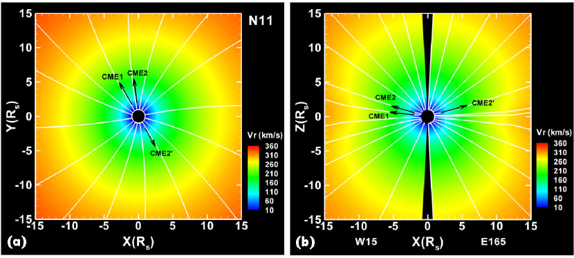
We first establish a steady state of background solar wind. The potential field extrapolated from the observed line-of-sight magnetic field on the photosphere and Parker’s solar wind solution are used as the initial magnetic field and velocity. The initial density is deduced from the momentum conservation law, and the initial temperature is given by assuming an adiabatic process. With these initial conditions, our MHD code may quickly reach a self-consistent and steady state of solar wind. Figure 1 presents the radial velocity of background solar wind and magnetic field lines, which shows the typical characteristics, e.g., nearly axial-symmetric and dipolar, at solar minimum.
| D | ||||||||||||
|---|---|---|---|---|---|---|---|---|---|---|---|---|
| km s-1 | cm-3 | K | nT | erg | ||||||||
| CME1 | N06W28 | 243 | 4.0 | 3.33 | 1.22 | 0.06 | 0.5 | 0.077 | 0.104 | 0.097 | 0.213 | |
| CME2 | N16W08 | 407 | 5.0 | 4.17 | 1.47 | 0.06 | 0.5 | 0.261 | 0.150 | 0.145 | 0.468 | |
| SW | N11W18 | 5.30 | 3.11 | 7.28 | 13.2 | |||||||
The columns from the second one to the right are the propagation direction, velocity, number density, temperature, magnetic field, plasma beta, radius, and the kinetic, magnetic, thermal, gravitational and total energies, respectively. The values of the velocity of solar wind are at and , respectively, in the direction of N11W18. The energies of solar wind are the integration over the whole computational domain before CMEs are introduced.
As we did in the previous work, two CMEs are modeled as magnetic blobs (Chané et al., 2005; Shen et al., 2011), and introduced successively with a separation time of 6 hours and their centers sitting at . Hereafter, we use CME1 and CME2 for the first and second initiated CMEs. To reproduce the 2008 November event, two key parameters, their initial propagation directions and velocities, are chosen to be the same as those derived from observations (C. Shen et al., 2012). The directions of the two CMEs are N06W28 and N16W08, respectively, and the propagation speeds are 243 and 407 km s-1, respectively. Another important parameter, plasma beta, is set a reasonable value of 0.06 for both CMEs. According to the analysis of errors in C. Shen et al. (2012), other parameters are not pivotal, and therefore set arbitrarily. Table 1 lists the initial parameters of the two CMEs.
3 Simulation results
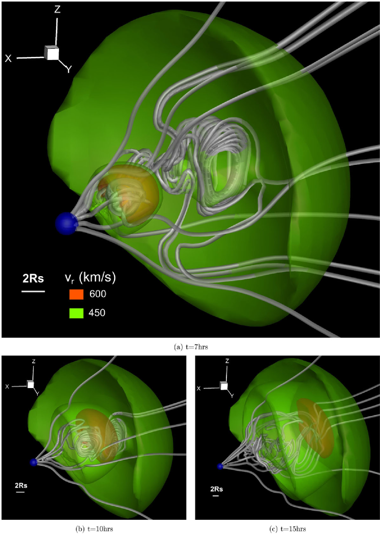
The background solar wind between the directions of the two CMEs gradually increases from about 316 km s-1 at to about 433 km s-1 at . Due to the expansion, the leading edges of the two CMEs move faster than ambient solar wind. Thus we locate the CMEs by simply setting a threshold of 450 km s-1 in the map of radial velocity. The time of introducing CME1 into computational domain is set to be zero. Figure 2 shows the 3-D view of the radial velocity distribution at 7, 10 and 15 hours, respectively. Only the regions of the radial velocity equal to 450 and 600 km s-1 are displayed for clarity. Due to the selection effect, some shell structures are shown, but they do not reflect the real CME shape. The CMEs can be recognized through the superimposed node-shaped magnetic field lines.
Since CME2 is faster than CME1, the two CMEs get closer and closer as shown in the three panels. The momentum transfer could be clearly seen by noting the orange region. At 7 hours, right before the collision, the orange region, which denotes a radial velocity of 600 km s-1, locates in CME2. After the two CMEs touch, the orange region moves forward, which suggests a momentum transfer from CME2 to CME1.
With some limits of the MHD code, however, we cannot identify the exact boundary of a CME. Thus we do not analyze the momentum or energy change for individual CMEs, but instead, analyze the variations of all kinds of energies integrated over the whole computational domain. All the energies of the two CMEs and solar wind at initial time are shown in Table 1. Although the energy of the two CMEs is only about 5% of the total energy of background solar wind, it is larger than the errors unavoidably from numerical calculations and ideal MHD assumptions as will be seen below.
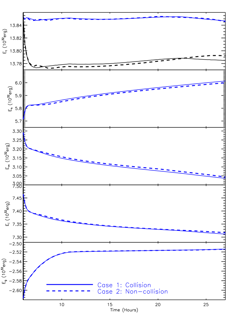
The solid black line in the upper panel of Figure 3 shows the variation of the total energy, , an integrated value over the whole computational domain, after the launch of CME2 at hours. The quick drop of at the beginning is because the introduced CME expels the ambient solar wind. This is a numerical effect and brings difficulty into the analysis of energy variation. To reduce it, we first calculate the net energy flowing into the computational domain at boundaries in a time interval , which is , where is the energy density at time and is the surface of the boundaries, and then deduct it from the total energy to get a corrected energy. Assume that the total energy at any given instant is and the net energy flow across the boundaries since the last instant is , the correct total energy is , which should be always equal to the total energy at initial time in theory. After the correction, the total energy varies in small range of about erg as shown by the solid blue line in the upper panel of Figure 3, that just indicates the numerical error in our simulation. It is much smaller than the CME energies listed in Table 1.
All kinds of energies after the correction are shown in the other panels in Figure 3. After the two CMEs propagate into the computational domain, the kinetic energy, , and gravitational energy, , both continuously increase, whereas the magnetic energy, , and thermal energy, , both decrease. The changes of these energies are all one order larger than the variation of total energy, suggesting a real physical process. The increase of is due to that the CMEs carry a heavier plasma than background solar wind. The changes of other energies are consistent with the well-known picture that CME’s magnetic and thermal energy will be converted into kinetic energy as it expands during the propagation (e.g., Kumar and Rust, 1996; Wang et al., 2009).
In order to validate that the kinetic energy gain (or partial of it) comes from a super-elastic collision, we need another case for comparison, in which the two CMEs do not collide. To do this, we adjust the longitude of CME2 to , which causes the longitudinal separation between the two CMEs to be , and keep all the other parameters exactly the same as those in the case of collision. Hereafter we use Case 1 for collision, Case 2 for non-collision and CME2′ for the second CME in Case 2. Figure 1 has shown that the background solar wind and magnetic structure around CME2 and CME2′ are quite similar. We believe that the two cases are comparable.
4 Comparison between the cases of collision and non-collision
From CME1 being introduced into computational domain to the instance of CME2 being introduced, the two cases are exactly the same. After CME2 is introduced, the two cases become different. The dashed blue lines in Figure 3 show the energy variations for Case 2, which are similar to those in Case 1 except some small differences. These small differences are shown much clearly in Figure 4.

The difference of the total energy, , between the two cases has small fluctuations with an amplitude of about erg. It indicates the level of numerical error. The difference of the gravitational energy, , is about erg, smaller than the numerical error. Thus we cannot conclude if is real or not. For all the other energies, the differences are significantly larger than the error, and thought to be physically meaningful.
It is found that, from the time of hours, the difference of the kinetic energy, , rapidly increases from about erg to about erg in 2 hours, and then decreases back to about erg and slowly returns. It means that there is extra kinetic energy gain in Case 1. Recall that the energy flow across the boundaries has been deducted, and therefore the extra kinetic energy gain must come from the collision of the two CMEs. Although we do not know the kinetic energy for each CME, the comparison between Case 2 and Case 1 is just like the comparison between the state before and after the collision. The significant difference between the two cases in the kinetic energy does confirm that the collision of CMEs could be super-elastic as suggested by C. Shen et al. (2012).
It is hard to identify when the collision ends. It might be at hours or even later. But we are sure that the two CMEs have fully interacted for a long time. This long process allows magnetic and thermal energies to be converted into kinetic energy. It is noticed that the decrease of the magnetic energy is much larger than that of the thermal energy, which suggests that the magnetic energy stored in CMEs are the major source of the extra kinetic energy gain.
5 Summary and discussion
We have comparatively investigated the energy variation during the collision of two successive CMEs. It is found that the kinetic energy gain in the case of collision is larger than that in the case of non-collision though the initial conditions of the two CMEs and the background solar wind are exactly the same. This result does suggest that the collision between the two CMEs is super-elastic, through which additional magnetic and thermal energies are converted into kinetic energy.
In this study, the initial kinetic energy of the two CMEs is about erg (see Table 1). Since the collision happens quickly after the introductions of the CMEs, we may use this value approximately as the CMEs’ kinetic energy right before the collision. The extra kinetic energy gain due to the collision is on the order of erg. It is therefore derived that the super-elastic collision of the two CMEs causes their total kinetic energy increased by about 3%–4%, which is close to the value of 6.6% given by C. Shen et al. (2012). Assuming the energy gain totally goes to CME1, we then estimate that the kinetic energy of CME1 increases by about 13%. Normally, the leading CME will be accelerated and the trailing CME decelerated (e.g., Wang et al., 2005; Shen et al., 2012; Lugaz et al., 2012). Thus the percentage of the kinetic energy gain of CME1 should be even higher. In terms of velocity, CME1 is speeded up by at least 6%, i.e., 15 km s-1. This number is not large enough to impact the space weather forecasting. But a comprehensive investigation of the effect of collision on the velocity and direction of CMEs is still worth being pursued.
In this letter, we only consider the CMEs similar to the 2008 November event. It is not clear if the collision between any CMEs is super-elastic. Moreover, some open questions remain. For example, how are the magnetic or thermal energies convert into kinetic energy? How does magnetic reconnection influence the collision process and result if it efficiently occurred? Another interesting thing is that the 2010 August event studied by Temmer et al. (2012) might be a case of ‘super-inelastic’ collision, a process somewhat like merging, of two fast CMEs. How and why could it happen? All these questions are worthy of further studies.
Acknowledgements.
This work is jointly supported by grants from the 973 key projects (2012CB825601, 2011CB811403), the CAS Knowledge Innovation Program (KZZD-EW-01-4), the NFSC (41031066, 41074121, 41231068, 41174150, 41274192, 41131065, 41121003 and 41274173), the Specialized Research Fund for State Key Laboratories, and the Public science and technology research funds projects of ocean (201005017).References
- Chané et al. (2005) Chané, E., C. Jacobs, B. Van der Holst, S. Poedts, and D. Kimpe, On the effect of the initial magnetic polarity and of the background wind on the evolution of CME shocks, Astron. & Astrophys., 432, 331–339, 2005.
- Farrugia and Berdichevsky (2004) Farrugia, C., and D. Berdichevsky, Evolutionary signatures in complex ejecta and their driven shocks, Ann. Geophys., 22, 3679–3698, 2004.
- Feng et al. (2003) Feng, X., S. T. Wu, F. Wei, and Q. Fan, A class of TVD type combined numerical scheme for MHD equations with a survey about numerical methods in solar wind simulations, Space Sci. Rev., 107, 43–53, 2003.
- Feng et al. (2005) Feng, X., C. Xiang, D. Zhong, and Q. Fan, A comparative study on 3-d solar wind structure observed by Ulysses and MHD simulation, Chinese Sci. Bull., 50, 672–678, 2005.
- Hayashi (2005) Hayashi, K., Magnetohydrodynamic simulations of the solar corona and solar wind using a boundary treatment to limit solar wind mass flux, Astrophys. J., 161, 480–494, 2005.
- Hayashi et al. (2006) Hayashi, K., X.-P. Zhao, and Y. Liu, MHD simulation of two successive interplanetary disturbances driven by cone-model parameters in IPS-based solar wind, Geophys. Res. Lett., 33, L20,103, 2006.
- Kumar and Rust (1996) Kumar, A., and D. M. Rust, Interplanetary magnetic clouds, helicity conservation, and current-core flux-ropes, J. Geophys. Res., 101, 15,667–15,684, 1996.
- Liu et al. (2012) Liu, Y. D., J. G. Luhmann, C. Möstl, J. C. Martínez-Oliveros, S. D. Bale, R. P. Lin, R. A. Harrison, M. Temmer, D. F. Webb, and D. Odstrcil, Interactions between coronal mass ejections viewed in coordinated imaging and in situ observations, Astrophys. J., 746, L15, 2012.
- Lugaz et al. (2005) Lugaz, N., I. Manchester, W. B., and T. I. Gombosi, Numerical simulation of the interaction of two coronal mass ejections from Sun to Earth, Astrophys. J., 634, 651–662, 2005.
- Lugaz et al. (2009) Lugaz, N., A. Vourlidas, and I. I. Roussev, Deriving the radial distances of wide coronal mass ejections from elongation measurements in the heliosphere application to CME-CME interaction, Ann. Geophys., 27, 3479–3488, 2009.
- Lugaz et al. (2012) Lugaz, N., C. J. Farrugia, J. A. Davies, C. Mostl, C. J. Davis, I. I. Roussev, and M. Temmer, The deflection of the two interacting coronal mass ejections of 2010 may 2324 as revealed by combined in situ measurements and heliospheric imaging, Astrophys. J., 759, 68(13pp), 2012.
- Reiner et al. (2003) Reiner, M. J., A. Vourlidas, O. C. St. Cyr, J. T. Burkepile, R. A. Howard, M. L. Kaiser, N. P. Prestage, and J.-L. Bougeret, Constraints on coronal mass ejection dynamics from simultaneous radio and white-light observations, Astrophys. J., 590, 533–546, 2003.
- C. Shen et al. (2012) Shen, C., Y. Wang, S. Wang, Y. Liu, R. Liu, A. Vourlidas, B. Miao, P. Ye, J. Liu, and Z. Zhou, Super-elastic collision of large-scale magnetized plasmoids in the heliosphere, Nature Phys., 8, 923–928, 2012.
- Shen et al. (2007) Shen, F., X. Feng, S. T. Wu, and C. Xiang, Three-dimensional MHD simulation of CMEs in three-dimensional background solar wind with the self-consistent structure on the source surface as input: Numerical simulation of the January 1997 Sun-Earth connection event, J. Geophys. Res., 112, A06,109, 2007.
- Shen et al. (2009) Shen, F., X. Feng, and W. B. Song, An asynchronous and parallel time-marching method: application to the three-dimensional MHD simulation of the solar wind, Science in china Series E: Technological Sciences, 52, 2895–2902, 2009.
- Shen et al. (2011) Shen, F., X. S. Feng, Y. Wang, S. T. Wu, W. B. Song, J. P. Guo, and Y. F. Zhou, Three-dimensional MHD simulation of two coronal mass ejections’ propagation and interaction using a successive magnetized plasma blobs model, J. Geophys. Res., 116, A09,103, 2011.
- Shen et al. (2012) Shen, F., S. T. Wu, X. Feng, and C.-C. Wu, Acceleration and deceleration of coronal mass ejections during propagation and interaction, J. Geophys. Res., 117, A11,101, 2012.
- Temmer et al. (2012) Temmer, M., B. Vršnak, T. Rollett, B. Bein, C. A. de Koning, Y. Liu, E. Bosman, J. A. Davies, C. Möstl, T. Žic, A. M. Veronig, V. Bothmer, R. Harrison, N. Nitta, M. Bisi, O. Flor, J. Eastwood, D. Odstrcil, and R. Forsyth, Characteristics of kinematics of a coronal mass ejection during the 2010 August 1 CME-CME interaction event, Astrophys. J., 749, 57, 2012.
- Wang et al. (2005) Wang, Y., H. Zheng, S. Wang, and P. Ye, MHD simulation of the formation and propagation of multiple magnetic clouds in the heliosphere, Astron. & Astrophys., 434, 309–316, 2005.
- Wang et al. (2009) Wang, Y., J. Zhang, and C. Shen, An analytical model probing the internal state of coronal mass ejections based on observations of their expansions and propagations, J. Geophys. Res., 114, A10,104, 2009.
- Wang et al. (2002) Wang, Y. M., S. Wang, and P. Z. Ye, Multiple magnetic clouds in interplanetary space, Sol. Phys., 211, 333–344, 2002.
- Wang et al. (2003) Wang, Y. M., P. Z. Ye, and S. Wang, Multiple magnetic clouds: Several examples during March – April, 2001, J. Geophys. Res., 108, 1370, 2003.
- Wu et al. (2007) Wu, C.-C., C. D. Fry, M. Dryer, S. T. Wu, B. Thompson, K. Liou, and X. S. Feng, Three-dimensional global simulation of multiple ICMEs interaction and propagation from the Sun to the heliosphere following the 25–28 October 2003 solar events, Adv. in Space Res., 40, 1827–1834, 2007.
- Wu and Wang (1987) Wu, S. T., and J. F. Wang, Numerical tests of a modified full implicit eulerian scheme with projected normal characteristic boundary conditions for MHD flows, Comput. Methods Appl. Mech. Eng., 24, 267–282, 1987.
- Wu et al. (2006) Wu, S. T., A. H. Wang, Y. Liu, and J. T. Hoeksema, Data driven magnetohydrodynamic model for active region evolution, Astrophys. J., 652, 800–811, 2006.
- Xiong et al. (2007) Xiong, M., H. Zheng, S. T. Wu, Y. Wang, and S. Wang, Magnetohydrodynamic simulation of the interaction between two interplanetary magnetic clouds and its consequent geoeffectiveness, J. Geophys. Res., 112, A11,103, 2007.