YITP-14-110

A review on SUSY gauge theories on $\bf S^{3}$

Kazuo Hosomichi

Department of Physics, National Taiwan University, Taipei 10617, Taiwan

abstract

We review the exact computations in 3D ${\cal N}=2$ supersymmetric gauge theories on the round or squashed $S^{3}$ and the relation between 3D partition functions and 4D superconformal indices. This is part of a combined review on the recent developments of the 2d-4d relation, edited by J. Teschner.

1 Introduction

Localization principle has been a powerful tool in the study of supersymmetric field theories which allows one to evaluate certain SUSY-preserving quantities by explicit path integration. It was first applied to 3D SUSY gauge theories on $S^{3}$ in [1], where a closed formula for partition function and Wilson loop was obtained for a class of ${\cal N}\geq 2$ superconformal Chern-Simons matter theories. With generalization by [2, 3], exact formula is now available for arbitrary 3D ${\cal N}=2$ SUSY gauge theories. The essential idea of localization is that, since nonzero contribution to supersymmetric path integrals arise only from SUSY invariant configurations of bosonic fields called saddle points, infinite dimensional path integrals can be reduced to finite-dimensional integrals over saddle points. It turned out that the analysis of 3D gauge theories on $S^{3}$ is much simpler than the case of 4D ${\cal N}=2$ SUSY gauge theories on $S^{4}$ [4] (see [V:5] for a review in this volume), due to the absence of saddle points with non-trivial topological quantum numbers.

The exact partition function, which depends on the radius of $S^{3}$ as well as some of the coupling constants, is one of the most basic quantities characterizing ${\cal N}=2$ supersymmetric theories. More informaition about the theories can be obtained by putting them on different 3D backgrounds preserving rigid supersymmetry and evaluating partition functions. In [5] it was shown that one can construct rigid ${\cal N}=2$ SUSY gauge theories on the ellipsoid $S^{3}_{b}$ with $U(1)\times U(1)$ isometry,

$$b^{2}(x_{0}^{2}+x_{1}^{2})+b^{-2}(x_{2}^{2}+x_{3}^{2})~{}=~{}1,$$ (1.1)

with a suitable background vector and scalar fields. The additional fields which are required to make the ellipsoid supersymmetric have their origin in the off-shell supergravity [6], where the fully generalized form of Killing spinor equation appears as local SUSY transformation laws of fermions in the supergravity multiplet. The ellipsoid partition function was shown to depend on the squashing parameter $b$ in a nontrivial manner. Another important background with rigid supersymmetry is $S^{2}\times S^{1}$ which leads to the path integral definition of the 3D superconformal index [7, 8]. There are also results on more general 3D manifolds with a slightly different formalism based on topological twist [9, 10].

Another useful approach to find supersymmetric deformations of the round $S^{3}$ is the Scherk-Schwarz like reduction of $S^{1}\times S^{3}$, which means that one includes finite rotation in the $S^{3}$ direction in the periodic identification of fields along $S^{1}$. This approach also makes an explicit connection between the 3D partition functions and 4D superconformal indices [11, 12, 13, 14], and in particular the relation between nonzero angular momentum fugacity in 4D and the deformed geometry in 3D [15, 16]. As was shown in [17, 18], the dimensional reduction results in the familiar squashed $S^{3}$ with $SU(2)\times U(1)$ isometry, with some additional background fields turned on. However, there are two inequivalent reductions whose effect on the 3D physical quantities are totally different.

Meanwhile, the study of certain domain walls in 4D ${\cal N}=2$ superconformal gauge theories in connection with AGT relation led to a conjecture that there is a precise agreement between quantities in 3D gauge theories on $S^{3}$ and the reprerentation theory of Virasoro or W algebras [19, 20]. In general, compactification of a $(2,0)$ theory on a Riemann surface $\Sigma$ gives rise to several different (Lagrangian) descriptions that are related to one another by S-duality [21]. The S-duality domain walls are defined by gluing two mutually S-dual theories along an interface, and therefore have a natural connection to the elements of the mapping class group or Moore-Seiberg groupoid operation acting on conformal blocks. In this respect, it is important that the squashing parameter $b$ corresponds to the Liouville or Toda coupling constant. Indeed, one of the building blocks of the ellipsoid partition function is the double-sine function $s_{b}(x)$, which in our context is most conveniently defined as the zeta-regularized infinite product [22]

$$s_{b}(x)~{}=~{}\prod_{m,n\in\mathbb{Z}_{\geq 0}}\frac{mb+nb^{-1}+\frac{Q}{2}-ix}{mb+nb^{-1}+\frac{Q}{2}+ix}.\quad\big{(}Q\equiv b+\frac{1}{b}\big{)}$$ (1.2)

The same function appears in the structure constants of Liouville or Toda CFTs with coupling $b$.

This review is organized as follows. In Section 2 we review the correspondence between a 3D gauge theory and 2D conformal field theories in the canonical example of the S-duality domain wall in ${\cal N}=2^{\ast}$ $SU(2)$ super Yang-Mills theory. In Section 3 we review the localization computation for 3D gauge theories on the round $S^{3}$ and the ellipsoid $S^{3}_{b}$, and summarize the formulae for partition function as well as expectation values of loop observables. In Section 4 we review the path integral computation of 4D superconformal index, and see how the squashed $S^{3}$ background arises as a result of Scherk-Schwarz reduction.

2 3D AGT relation

We review here the correspondence between 3D gauge theories and 2D conformal field theories in one typical example. The original idea was given in [19] which discussed the S-duality domain walls in 4D ${\cal N}=2$ superconformal theories of class S, namely the compactification of $(2,0)$-theories on punctured Riemann surfaces (see [V:1] for a review). It is important to recall here that, for this class of theories, there are different gauge theory descriptions corresponding to different pants decomposition $\sigma$ of the surface $\Sigma$, and they are equivalent (S-dual) to one another. Also, if Lagrangian description is available, its gauge coupling $q$ is determined from the complex structure of $\Sigma$ which we regard to take values in Teichmüller space.

2.1 Janus and S-duality domain walls

A Janus domain wall is a supersymmeric deformation of gauge theories which makes the complexified gauge coupling jump across the wall. Consider a theory of class S on $S^{4}$ with a Janus wall along the equator $S^{3}$ where the two (left and right) hemispheres with couplings $q$ and $q^{\prime}$ meet. The 4D partition function in the presence of the wall should be given by

$$Z~{}=~{}\int d\nu(a)\ {\cal F}^{(\sigma)}_{a,m}(\bar{q}){\cal F}^{(\sigma)}_{a,m}(q^{\prime}),$$ (2.1)

as the product of the instanton partition functions ${\cal F}$ integrated over the real Coulomb branch parameters $a$ with an appropriate measure. Here $m$ denotes a collection of mass parameters, and $\sigma$ labels a choice of pants decomposition. For generic complex structure $q$ there is a natural pants decomposition which leads to a weakly coupled gauge theory description, and we choose $\sigma$ to be the natural one at $q$.

As $q^{\prime}$ is varied away from $q$, the gauge theory on the right hemisphere becomes strongly coupled. To analytically continue the formula (2.1) in such a situation, one needs to S-dualize the right hemisphere and move to another pants decomposition $\sigma^{\prime}$ which gives a weakly coupled description at $q^{\prime}$. We then have a system of two mutually S-dual theories meeting along the so-called S-duality domain wall. In the special case where $q^{\prime}$ is an image of $q$ under the mapping class group, $\sigma$ and $\sigma^{\prime}$ are equivalent so the theories on the two sides of the wall are the same. However, their degrees of freedom are connected across the wall via S-duality.

Under the AGT relation, the instanton partition functions correspond to Liouville or Toda conformal blocks labeled by a fusion channel $\sigma$ and the internal and external momenta $a,m$. They should therefore transform under S-duality in the same way that the corresponding conformal blocks transform under the Moore-Seiberg groupoid operation $g$,

$${\cal F}_{a,m}^{(\sigma)}(q^{\prime})~{}=~{}\int d\nu(a^{\prime})\,g_{a,a^{\prime},m}\,{\cal F}_{a^{\prime},m}^{(\sigma^{\prime})}(q^{\prime}).$$ (2.2)

By substituting (2.2) into (2.1) we obtain a formula for the $S^{4}$ partition function in the presence of an S-duality domain wall. Now the integration variables get doubled, as the Coulomb branch parameters on the two sides of the wall can vary independently. At this point, it is natural to expect that the integration kernel $g_{a,a^{\prime},m}$ in (2.2) corresponds to the degrees of freedom localized on the S-duality wall between the two 4D theories in their vacua $a,a^{\prime}$.

In general, the S-duality walls should be described by some local 3D worldvolume field theories coupled to the 4D bulk degrees of freedom. In the following we take the example of ${\cal N}=2^{\ast}$ SYM theory, which is a deformation of ${\cal N}=4$ SYM by a mass of the adjoint hypermultiplet. The S-duality transformations for this theory form the group $SL(2,\mathbb{Z})$ and we are interested in the wall corresponging to the “$S$-element”. For $SU(N)$ gauge group, we expect the correspondence with the $A_{N-1}$ Toda theory on a one-punctured torus. In the Liouville case $N=2$, the kernel for the S-duality operation acting on torus 1-point conformal block is known explicitly [23],

$$g_{(p,p^{\prime},p_{E})}=\frac{2^{\frac{3}{2}}}{s_{b}(p_{E})}\int_{\mathbb{R}}{\rm d}\sigma\frac{s_{b}(p^{\prime}+\sigma+\frac{1}{2}p_{E}+\frac{iQ}{4})}{s_{b}(p^{\prime}+\sigma-\frac{1}{2}p_{E}-\frac{iQ}{4})}\frac{s_{b}(p^{\prime}-\sigma+\frac{1}{2}p_{E}+\frac{iQ}{4})}{s_{b}(p^{\prime}-\sigma-\frac{1}{2}p_{E}-\frac{iQ}{4})}e^{4\pi ip\sigma}.$$ (2.3)

Here $b$ is the Liouville coupling and $Q\equiv b+b^{-1}$. The Liouville momenta $p,p^{\prime},p_{E}$ are related to the conformal weight $h$ labeling the Virasoro highest weight representations by the formula $h=p^{2}+Q^{2}/4$. The double-sine function $s_{b}(x)$ is defined by (1.2), and will appear frequently later in this article.

2.2 Example: ${\cal N}=2^{\ast}$ SYM

A classification of boundary conditions and domain walls for ${\cal N}=4$ SYM theories with general gauge group $G$ was given in [24, 25], and the action of S-duality on these objects was also studied. The 3D theory on the S-duality domain walls, called $T[G]$, plays a central role in this story. For $SU(N)$ gauge group, it was shown that the wall theory $T[SU(N)]$ is given by a 3D ${\cal N}=4$ SUSY quiver gauge theory corresponding to the diagram in the left of Figure 1.

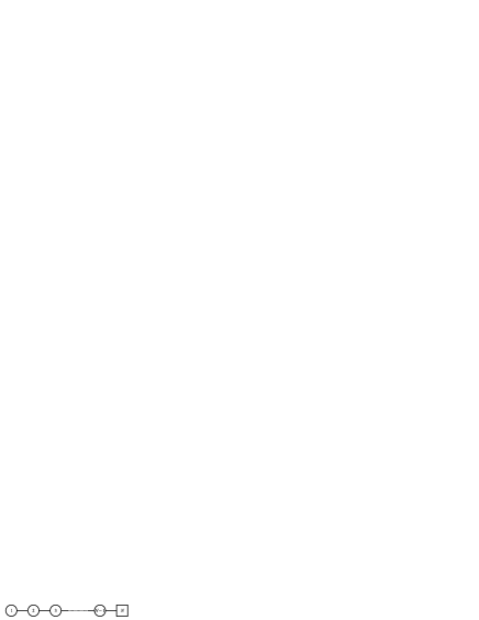
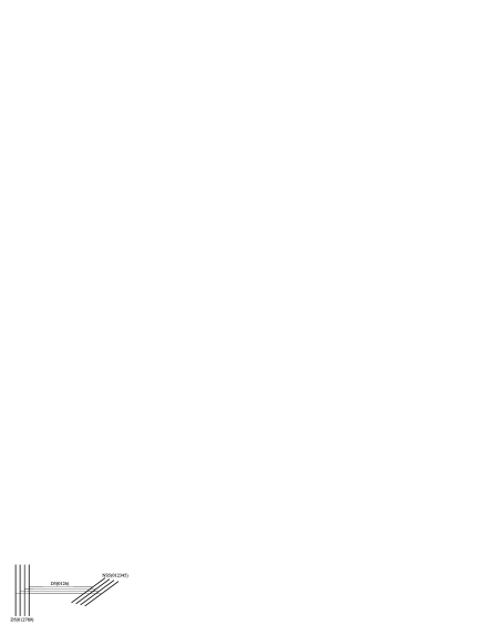
Figure 1: The quiver diagram and a type IIB brane construction for the 3D gauge theory $T[SU(N)]$.

Here the circles and the square correspond respectively to the gauge symmetry $U(1)\times U(2)\times\cdots\times U(N-1)$ and a global $U(N)$ symmetry, and the links correspond to hypermultiplets. The Coulomb and Higgs branch moduli spaces both have an $SU(N)$ symmetry which can be coupled to the gauge fields in the bulk.

A simple type IIB brane construction can reproduce this fact. Consider $N$ D3-branes stretched along the directions 0126 with $-L\leq x_{6}\leq L$, ending on the D5-branes at $x_{6}=\pm L$ extending in the directions 012789. Due to the boundary condition at D5-branes, the massless modes on D3-brane wordlvolume decompose into 3D ${\cal N}=4$ vector and hypermultiplets. The vectormultiplet fields obey Dirichlet boundary condition, so for small $L$ they are frozen to take vacuum configuration. As was explained in [24], to avoid D3-branes developing Nahm poles at the boundary, we need to introduce $N$ D5-branes at each end so that each D5-brane has precisely one D3-brane ending on it. Nonzero (real) Coulomb branch parameter $a$ can then be introduced by putting the $i$-th D5-branes at, say, $(x_{3},x_{4},x_{5})=(a_{i},0,0)$ at each end.

Consider next the same brane configuration but now with an S-duality domain wall on the D3-brane worldvolume at $x_{6}=0$. It can be eliminated by applying the type IIB S-duality combined with the exchange of 345 and 789 directions to the right half space $x_{6}\geq 0$, but then the $N$ D5-branes at $x_{6}=L$ turn into $N$ NS5-branes (012345). The resulting brane configuration as shown on the right of Figure 1 is what precisely gives rise to the above-mentioned quiver gauge theory. The D5-branes and NS5-branes are now free to move independently. The positions of NS5-branes $a$ turn into $N-1$ Fayet-Iliopoulos parameters, whereas those of D5-branes $a^{\prime}$ determine the masses of the $U(N-1)\times U(N)$ bifundamental hypermultiplets.

Let us now focus on the simplest nontrivial case $N=2$. In 3D ${\cal N}=2$ terminology, the wall theory $T[SU(2)]$ is a $U(1)$ gauge theory with five chiral multiplets $\phi,q_{1},q_{2},\tilde{q}^{1},\tilde{q}^{2}$. The neutral chiral field $\phi$ is a part of ${\cal N}=4$ $U(1)$ vector multiplet and has R-charge 1. The two electrons $q_{1},q_{2}$ and the two positrons $\tilde{q}^{1},\tilde{q}^{2}$ have the R-charge $1/2$, and they form two flavors of hypermultiplets. ${\cal N}=4$ supersymmetry requires a cubic superpotential of the form $\tilde{q}^{i}\phi q_{i}$.

As we have seen, the Coulomb branch parameter $a$ appears in the wall theory as the $U(1)$ FI parameter, while $a^{\prime}$ is the mass for charged chiral fields which breaks the $SU(2)$ flavor symmetry to $U(1)$. In addition, the bulk ${\cal N}=2^{\ast}$ mass parameter $m$ should also show up in the wall theory in a way that preserves 3D ${\cal N}=2$ supersymmetry as well as the $SU(2)$ isometries of the Coulomb and Higgs branches. It was argued in [20] that $m$ is the mass for the chiral fields associated to the global symmetry under which $q_{i},\tilde{q}^{i}$ have charge $+1$ and $\phi$ has charge $-2$.

It was observed in [20] that the exact partition function of this mass-deformed $T[SU(2)]$ theory on $S^{3}$ agrees precisely with the kernel of the S-duality transformation (2.3) for $b=1$, under the identification

$$p=a,\quad p^{\prime}=a^{\prime},\quad p_{E}=m.$$ (2.4)

It was then shown in [5] that the formula (2.3) for general values of the coupling $b$ can be reproduced by deforming the round $S^{3}$ into an ellipsoid $S^{3}_{b}$. The derivation of the formulae which are necessary to confirm this agreement will be reviewed in the next section.

2.3 A 3D picture

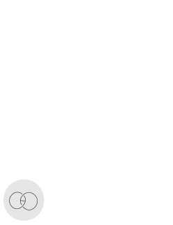
Figure 2: (left) the process of a one-punctured torus degenerating into a Moore-Seiberg graph, thereby sweeping out a solid torus with a network of defect inside. (right) Two such solid tori glued together to make an $S^{3}$ with a network of defect.

As we have seen, Janus or S-duality domain walls correspond to smooth evolutions of the complex structure of a surface, and therefore have an interpretation as M5-branes wrapping three-manifolds. Let us explain this in the example of ${\cal N}=2^{\ast}$ SYM.

Consider a Janus domain wall corresponding to a path in Teichmüller space between two points of extreme weak coupling that are S-dual image of each other. As one approaches towards one end from any point along the path, the torus $\Sigma$ becomes thinner and thinner until it looks like the Moore-Seiberg graph $\Gamma_{1}$ for the torus one-point conformal blocks. In this process, two-dimensional part of the M5-brane worldvolume sweeps out a 3D solid torus $B_{1}$ with a codimension-2 defect $\Gamma_{1}$ left inside (Figure 2 left). One of the two basis 1-cycles $\alpha,\beta$ of the torus, say $\alpha$, shrinks to zero length inside $B_{1}$. Starting from the same point on the path and moving toward the other end, one obtains another solid torus $B_{2}$ with a defect $\Gamma_{2}$, inside which the cycle $\beta$ shrinks to zero length. The two solid tori $B_{1}$ and $B_{2}$ glued together makes an $S^{3}$ with a defect $\Gamma$ which is the union of the two graphs $\Gamma_{1},\Gamma_{2}$ joined at the external legs (Figure 2 right). $\Gamma$ therefore consists of two circle defects and a segment connecting them, and the three components are naturally labeled by the momenta $p,p^{\prime},p_{E}$.

The 3D theories on domain walls or boundaries of 4D class S theories are now regarded as part of a much bigger class of theories which arise from M5-branes wrapping hyperbolic 3-manifolds. The relation between 3D SUSY gauge theories and hyperbolic 3-manifolds also gives rise to an AGT-like correspondence between 3D supersymmetric theories and Chern-Simons theories with non-compact gauge groups. For more details on this topic, see the review [V:10] in this volume.

3 3D Partition Function

In this section we review the construction of 3D ${\cal N}=2$ supersymmetric gauge theories on a class of rigid SUSY backgrounds. Then we concentrate on the theories on the round sphere and the ellipsoids, and show how to compute partition function as well as the expectation values of Wilson and vortex loops using localization principle.

3.1 3D ${\cal N}=2$ SUSY theories

Let us begin by summarizing our convention for 3D spinor calculus. We use the standard Pauli’s matrices for the Dirac matrices $\gamma^{a}$, and also $\gamma^{ab}=\frac{1}{2}(\gamma^{a}\gamma^{b}-\gamma^{b}\gamma^{a})$. To define bilinear products of spinors, we use an anti-symmetric $2\times 2$ matrix $C$ with nonzero elements $C_{12}=-C_{21}=1$. Writing the spinor indices explicitly, various bilinears are defined as follows.

$$\epsilon\psi\equiv\epsilon^{\alpha}C_{\alpha\beta}\psi^{\beta},\quad\epsilon\gamma^{a}\psi\equiv\epsilon^{\alpha}C_{\alpha\beta}(\gamma^{a})^{\beta}_{~{}\gamma}\psi^{\gamma},\quad\text{etc.}$$ (3.1)

In rigid SUSY theories on curved backgrounds, the parameters of SUSY transformation $\epsilon$ are no longer constants, but are solutions to the Killing spinor equation. For 3D ${\cal N}=2$ supersymmetric theories, the SUSY is parametrized by two Killing spinors $\epsilon,\bar{\epsilon}$ of R-charge $+1,-1$. The most general form of the Killing spinor equation can be found from off-shell supergravity [26] as the condition that gravitini are invariant under local SUSY for a suitable choice of parameters $\epsilon,\bar{\epsilon}$.

$$D_{m}\epsilon = \Big{(}\partial_{m}+\frac{1}{4}\omega_{m}^{ab}\gamma^{ab}-iV_{m}\Big{)}\epsilon~{}=~{}iM\gamma_{m}\epsilon-iU_{m}\epsilon-\frac{1}{2}\varepsilon_{mnp}U^{n}\gamma^{p}\epsilon,$$

$$D_{m}\bar{\epsilon} = \Big{(}\partial_{m}+\frac{1}{4}\omega_{m}^{ab}\gamma^{ab}+iV_{m}\Big{)}\bar{\epsilon}~{}=~{}iM\gamma_{m}\bar{\epsilon}+iU_{m}\bar{\epsilon}+\frac{1}{2}\varepsilon_{mnp}U^{n}\gamma^{p}\bar{\epsilon}.$$ (3.2)

Here $\gamma_{m}\equiv e^{a}_{m}\gamma^{a}$ with $e^{a}_{m}$ the vielbein, and throughout this article we regard $\epsilon,\bar{\epsilon}$ as Grassmann even. Supersymmetric backgrounds are therefore characterized by the metric as well as the $U(1)_{\text{R}}$ gauge field $V_{m}$ and other auxiliary fields $M,U_{m}$ in the off-shell gravity multiplet. In this section we restrict our discussion to the backgrounds with

$$U_{m}=0,$$ (3.3)

which include the round sphere and ellipsoids. More general supersymmetric backgrounds were studied systematically in three and four dimensions in [27, 28, 26, 29]. For 3D ${\cal N}=2$ systems it was shown that the existence of a Killing spinor implies that the background admits an almost contact metric structure.

The fields in 3D ${\cal N}=2$ theories are grouped into two kinds of supermultiplets. A vector multiplet consists of a vector $A_{m}$, a real scalar $\sigma$, a pair of spinors $\lambda,\bar{\lambda}$ and an auxiliary scalar $D$ which are all Lie algebra valued. They transform under supersymmetry as

$$\delta A_{m} = -\frac{i}{2}(\epsilon\gamma_{m}\bar{\lambda}+\bar{\epsilon}\gamma_{m}\lambda),$$

$$\delta\sigma = \frac{1}{2}(\epsilon\bar{\lambda}-\bar{\epsilon}\lambda),$$

$$\delta\lambda = \frac{1}{2}\gamma^{mn}\epsilon F_{mn}-\epsilon D-i\gamma^{m}\epsilon D_{m}\sigma,$$

$$\delta\bar{\lambda} = \frac{1}{2}\gamma^{mn}\bar{\epsilon}F_{mn}+\bar{\epsilon}D+i\gamma^{m}\bar{\epsilon}D_{m}\sigma,$$

$$\delta D = \frac{i}{2}\epsilon\Big{(}\gamma^{m}D_{m}\bar{\lambda}+[\sigma,\bar{\lambda}]+iM\bar{\lambda}\Big{)}-\frac{i}{2}\bar{\epsilon}\Big{(}\gamma^{m}D_{m}\lambda-[\sigma,\lambda]+iM\lambda\Big{)}.$$ (3.4)

A chiral multiplet consists of a scalar $\phi$, a spinor $\psi$ and an auxiliary scalar $F$ in an arbitrary representation $R$ of the gauge group. Their conjugate fields $(\bar{\phi},\bar{\psi},\bar{F})$ are in the conjugate representation $\bar{R}$. If one assign the R-charge $r$ to $\phi$ and $-r$ to $\bar{\phi}$, the R-charge of the remaining fields is determined from the supersymmetry as in Table 1.

fields	$\epsilon$	$\bar{\epsilon}$	$A_{a}$	$\sigma$	$\lambda$	$\bar{\lambda}$	$\tilde{D}$	$\phi$	$\bar{\phi}$	$\psi$	$\bar{\psi}$	$F$	$\bar{F}$
weight	$-\frac{1}{2}$	$-\frac{1}{2}$	$1$	$1$	$\frac{3}{2}$	$\frac{3}{2}$	$2$	$r$	$r$	$r+\frac{1}{2}$	$r+\frac{1}{2}$	$r+1$	$r+1$
R-charge	$1$	$-1$	$0$	$0$	$1$	$-1$	$0$	$r$	$-r$	$r-1$	$1-r$	$r-2$	$2-r$

Table 1: the scaling weight and the R-charge of the fields.

The transformation rule for these fields is given by

$$\delta\phi = \epsilon\psi,\quad\delta\psi~{}=~{}i\gamma^{m}\bar{\epsilon}D_{m}\phi+i\bar{\epsilon}\sigma\phi+\frac{2ri}{3}\gamma^{m}D_{m}\bar{\epsilon}\phi+\epsilon F,$$

$$\delta\bar{\phi} = \bar{\epsilon}\bar{\psi},\quad\delta\bar{\psi}~{}=~{}i\gamma^{m}\epsilon D_{m}\bar{\phi}+i\epsilon\bar{\phi}\sigma+\frac{2ri}{3}\gamma^{m}D_{m}\epsilon\bar{\phi}+\bar{\epsilon}\bar{F},$$

$$\delta F = \bar{\epsilon}(i\gamma^{m}D_{m}\psi-i\sigma\psi-i\bar{\lambda}\phi)+\frac{i}{3}(2r-1)D_{m}\bar{\epsilon}\gamma^{m}\psi,$$

$$\delta\bar{F} = \epsilon(i\gamma^{m}D_{m}\bar{\psi}-i\bar{\psi}\sigma+i\bar{\phi}\lambda)+\frac{i}{3}(2r-1)D_{m}\epsilon\gamma^{m}\bar{\psi}.$$ (3.5)

Here the quantities in the representation $R$ ($\bar{R}$) are regarded as the column vectors (resp. row vectors), so that the vector multiplet fields act on them from the left (right).

Supersymmetric Lagrangian consists of the following invariants. Those involving only vector multiplet fields are the Chern-Simons term (for which we write the action integral),

$$S_{\text{CS}}~{}=~{}\frac{ik}{4\pi}\int\text{Tr}\bigg{(}A{\rm d}A-\frac{2i}{3}A^{3}-\sqrt{g}{\rm d}^{3}x\left(\bar{\lambda}\lambda+2\sigma D+4M\sigma^{2}\right)\bigg{)},$$ (3.6)

the Yang-Mills term and the Fayet-Iliopoulos term for abelian gauge symmetry.

$${\cal L}_{\text{g}} = {\rm Tr}\bigg{(}\frac{1}{2}F_{mn}F^{mn}+D_{m}\sigma D^{m}\sigma+D^{2}+i\bar{\lambda}\gamma^{m}D_{m}\lambda-i\bar{\lambda}[\sigma,\lambda]-M\bar{\lambda}\lambda\bigg{)},$$

$${\cal L}_{\text{FI}} = -\frac{i\zeta}{\pi}\left(D+4M\sigma\right).$$ (3.7)

The kinetic term for chiral matters is given by

$${\cal L}_{\text{m}} = D_{m}\bar{\phi}D^{m}\phi+\bar{\phi}\sigma^{2}\phi+4i(r-1)M\bar{\phi}\sigma\phi-2r(2r-1)M^{2}\bar{\phi}\phi+\frac{rR}{4}\bar{\phi}\phi-i\bar{\phi}D\phi$$ (3.8)

$$+\bar{F}F-i\bar{\psi}\gamma^{m}D_{m}\psi+i\bar{\psi}\sigma\psi-(2r-1)M\bar{\psi}\psi+i\bar{\psi}\bar{\lambda}\phi-i\bar{\phi}\lambda\psi\,,$$

with $R$ the scalar curvature of the background. The F-term of gauge invariant products of chiral multiplets with R-charge $r=2$ is also invariant, but one can show that the result of localization computation does not depend on the F-term couplings. Note that, while the bosonic part of ${\cal L}_{\text{g}}$ is positive definite, that of ${\cal L}_{\text{m}}$ has positive definite real part only when the value of $r$ is chosen appropriately. For example, for round sphere the positivity holds only when $0<r<2$.

The real mass for matters can be introduced by gauging the flavor symmetry by a background vector multiplet. The value of the background fields is chosen so as to preserve supersymmetry,

$$\sigma^{\text{(bg)}}=m~{}\text{(constant)},\quad D^{\text{(bg)}}=A_{m}^{\text{(bg)}}=\lambda^{\text{(bg)}}=\bar{\lambda}^{\text{(bg)}}=0.$$ (3.9)

3.2 SUSY localization

To apply localization principle to supersymmetric path integrals, one first chooses an arbitrary supercharge $\delta$, and then argue that the nonzero contribution to the path integral can be localized to the vicinity of saddle points, namely bosonic field configurations invariant under $\delta$. This means that $\delta$-transform of all the fermions must vanish on saddle points. For the theories of our interest, a useful observation is that both ${\cal L}_{\text{g}}$ and ${\cal L}_{\text{m}}$ are SUSY exact for any choice of $\delta$, which follows from

$$\bar{\epsilon}\epsilon\cdot{\cal L}_{\text{g}} = \delta_{\epsilon}\delta_{\bar{\epsilon}}{\rm Tr}\left(\bar{\lambda}\lambda+4D\sigma+8M\sigma^{2}\right)\,,$$

$$\bar{\epsilon}\epsilon\cdot{\cal L}_{\text{m}} = \delta_{\epsilon}\delta_{\bar{\epsilon}}\left(\bar{\psi}\psi-2i\bar{\phi}\sigma\phi+4M(r-1)\bar{\phi}\phi\right)\,.$$ (3.10)

Namely, they can be written as $\delta$-variation of some fermionic quantities, so they have to vanish at saddle points. A necessary condition for vector multiplet fields at saddle points follows from ${\cal L}_{\text{g}}=0$,

$$F_{mn}=D_{m}\sigma=D=0.$$ (3.11)

This is actually sufficient for the saddle point condition $\delta\lambda=\delta\bar{\lambda}=0$ to be satisfied. For theories on the round $S^{3}$ or its deformations, saddle points are thus labeled by constant scalar field $\sigma$ and vanishing gauge field, up to gauge transformations. For non-simply connected manifolds such as lens spaces, one also has choices of Wilson lines along non-contractible loops [30, 31, 32]. For matter multiplets, an obvious solution to $\delta\psi=\delta\bar{\psi}=0$ is

$$\phi=\bar{\phi}=F=\bar{F}=0.$$ (3.12)

To show that this is the unique saddle point, the simplest way is to check that the kinetic operator for $\phi$ in ${\cal L}_{\text{m}}$ has no zeromodes, so that ${\cal L}_{\text{m}}$ vanishes only at (3.12). For theories on the round sphere, one can show by a full spectrum analysis that there are no zeromodes on all the saddle points as long as $0<r<2$. This allows us to assume that the spectrum remains free of zeromodes on the ellipsoids $S^{3}_{b}$ as long as $b$ is reasonably close to $1$. The exact partition function on $S^{3}_{b}$ turns out to be analytic in $b$, so it can be continued to arbitrary $b>0$.

Since ${\cal L}_{\text{g}}$ and ${\cal L}_{\text{m}}$ are exact, the value of supersymmetric path integrals does not change if one adds them to the original Lagrangian with arbitrary coefficients $t_{\text{g}},t_{\text{m}}$. By making those coefficients very large, one can bring the theory into extreme weak coupling. In this limit the path integral simplifies and can be performed in two steps. One first integrates over fluctuations around each saddle point, for which Gaussian approximation is exact. The result is then integrated over the space of saddle points labeled by constant $\sigma$.

3.3 Partition function on the round sphere

As the simplest and yet the most important case, let us reproduce here the exact partition function of general ${\cal N}=2$ SUSY theories on the unit round $S^{3}$.

We write the unit round metric as ${\rm d}s^{2}=e^{a}e^{a}$, and identify the dreibein $e^{a}=e^{a}_{m}{\rm d}x^{m}$ with the left-invariant one-forms on the $SU(2)$ group manifold via

$$g^{-1}{\rm d}g=ie^{a}\gamma^{a},\quad g\in SU(2).$$ (3.13)

The isometry $SU(2)_{\mathscr{L}}\times SU(2)_{\mathscr{R}}$ acts on $g$ from its left and right. Note that, under the above choice of the local Lorentz frame, $SU(2)_{\mathscr{R}}$ acts on fields as local Lorentz rotation as well as isometry rotation.

Let us summarize here the spectrum of free fields on the round sphere. We first notice that one can use the inverse dreibein $e^{am}$ to define a triplet of vector fields $\mathscr{R}^{a}\equiv\frac{1}{2i}e^{am}\partial_{m}$ which generates $SU(2)_{\mathscr{R}}$. Using them, the kinetic terms for free complex scalars and spinors can be rewritten as

$$\bar{\phi}\;\Delta_{S^{3}}^{\text{scalar}}\phi \equiv g^{mn}\partial_{m}\bar{\phi}\partial_{n}\phi~{}=~{}\bar{\phi}\cdot 4\mathscr{R}^{a}\mathscr{R}^{a}\phi,$$

$$-i\bar{\psi}\;/\!\!\!\!D_{S^{3}}\psi \equiv -i\bar{\psi}\gamma^{m}D_{m}\psi~{}=~{}\bar{\psi}(4S^{a}\mathscr{R}^{a}+\tfrac{3}{2})\psi,$$ (3.14)

where $S^{a}=\frac{1}{2}\gamma^{a}$ is the generator of local Lorentz $SU(2)$ acting on spinors. Likewise, for a free Maxwell field $A=A^{a}e^{a}$ and its field strength $\ast{\rm d}A=F^{a}e^{a}$, one finds

$$F^{a}~{}=~{}2i\varepsilon^{abc}\mathscr{R}^{b}A^{c}+2A^{a},~{}~{}\text{or}\quad\vec{F}=(2+2\mathscr{R}^{a}T^{a})\vec{A},$$ (3.15)

where $T^{a}$ is the generator of local Lorentz $SU(2)$ in the triplet representation. The Maxwell kinetic operator for gauge field is given by $\Delta_{S^{3}}^{\text{vector}}\equiv(\ast{\rm d})^{2}$. The space of scalar, spinor and vector wave functions on $S^{3}$ thus form the following representation of $SU(2)_{\mathscr{L}}\times SU(2)_{\mathscr{R}}$.

$${\cal H}_{\text{scalar}} = \bigoplus_{n\geq 0}(\tfrac{n}{2},\tfrac{n}{2})_{n(n+2)},$$

$${\cal H}_{\text{spinor}} = \bigoplus_{n\geq 0}\Big{\{}(\tfrac{n}{2},\tfrac{n+1}{2})_{n+3/2}\oplus(\tfrac{n+1}{2},\tfrac{n}{2})_{-n-3/2}\Big{\}},$$

$${\cal H}_{\text{vector}} = \bigoplus_{n\geq 0}\Big{\{}(\tfrac{n}{2},\tfrac{n+2}{2})_{(n+2)^{2}}\oplus(\tfrac{n+1}{2},\tfrac{n+1}{2})_{0}\oplus(\tfrac{n+2}{2},\tfrac{n}{2})_{(n+2)^{2}}\Big{\}}.$$ (3.16)

For convenience, we put the eigenvalue of $\Delta_{S^{3}}^{\text{scalar}},-i\;/\!\!\!\!D_{S^{3}}$ or $\Delta_{S^{3}}^{\text{vector}}$ for each irreducible representation as suffix. Note that the nonzero eigenmodes of $\Delta_{S^{3}}^{\text{vector}}$ are divergenceless vectors while the zero eigenmodes are total divergences.

On the unit round $S^{3}$, the simplest form of the Killing spinor equation

$$\Big{(}\partial_{m}+\frac{1}{4}\omega_{m}^{ab}\gamma^{ab}\Big{)}\epsilon~{}=~{}iM\gamma_{m}\epsilon,\quad M=\pm\frac{1}{2}$$ (3.17)

has solutions. First, in the left-invariant local Lorentz frame, any constant spinor satisfies (3.17) with $M=+\frac{1}{2}$. The two independent solutions are left-invariant and transform as a doublet of $SU(2)_{\mathscr{R}}$. In addition, there are two independent solutions to (3.17) with $M=-\frac{1}{2}$ both of which are given by $g^{-1}$ times a constant spinor. They are therefore right-invariant and form an $SU(2)_{\mathscr{L}}$ doublet. In this subsection, we choose the background $V_{m}=0,M=\frac{1}{2}$.

Let us now turn to the computation of partition function using the localization principle. The supersymmetric saddle points are labeled by the constant value of the vector multiplet scalar $\sigma(x)=a$. The Chern-Simons or Fayet-Iliopoulos Lagrangians take nonzero value at the saddle point $a$ according to the formula

$$e^{-S_{\text{CS}}}=e^{i\pi k\text{Tr}(a^{2})},\quad e^{-S_{\text{FI}}}=e^{4\pi i\zeta a},$$ (3.18)

In addition, we need the one-loop determinant which arise from integrating over all the fluctuation modes at the saddle point $a$ under Gaussian (=one-loop) approximation.

We first study the vector multiplet for a non-abelian gauge symmetry $G$. Following the general prescription, we add to the original Lagrangian a SUSY exact regulator term $t_{\text{g}}{\cal L}_{\text{g}}$ and take $t_{\text{g}}\to\infty$. In this limit the regulator term dominates the path integral weight, and the Gaussian approximation becomes exact. The quadratic part of ${\cal L}_{\text{g}}$ in the Lorentz gauge $\partial^{m}A_{m}=0$ is

$${\cal L}_{\text{g}}~{}=~{}{\rm Tr}\bigg{[}\vec{A}\big{(}\Delta_{S^{3}}^{\text{vector}}+a_{\text{adj}}^{2}\big{)}\vec{A}+\hat{\sigma}\Delta_{S^{3}}^{\text{scalar}}\hat{\sigma}+D^{2}-\bar{\lambda}\big{(}-\!i\;/\!\!\!\!D_{S^{3}}+\tfrac{1}{2}+ia_{\text{adj}}\big{)}\lambda\bigg{]}.$$ (3.19)

Here we introduced the notation $a_{\text{adj}}$ for $a$ in the adjoint representation, namely $a_{\text{adj}}\lambda\equiv[a,\lambda]$, and $\hat{\sigma}$ denotes the fluctuation of $\sigma$ around its saddle point value $a$. To fix the gauge, we express the gauge field $A$ as a sum of a divergenceless vector field $\hat{A}$ and a total derivative ${\rm d}\varphi$, and insert the delta functional for $\varphi$. The Faddeev-Popov ghost determinant is trivial since gauge symmetry is just the shift of $\varphi$ (up to terms irrelevant in the saddle-point approximation). But since ${\rm Tr}A_{m}A^{m}={\rm Tr}(\hat{A}_{m}\hat{A}^{m}+\partial_{m}\varphi\partial^{m}\varphi)$, this change of integration variables gives rise to a Jacobian

$$\mathscr{D}A~{}=~{}\mathscr{D}\hat{A}\mathscr{D}^{\prime}\varphi\cdot(\text{Det}^{\prime}\Delta_{S^{3}}^{\text{scalar}})^{\frac{1}{2}{\rm dim}G},$$ (3.20)

where the primes indicate that the constant modes are excluded. This Jacobian is canceled against the determinant arising from $\hat{\sigma}$-integration.

The integration over the remaining physical fields $\lambda,\bar{\lambda}$ and $\hat{A}$ gives rise to the following ratio of determinants,

$$Z^{\text{1-loop}}_{\text{vec}} = \frac{\text{det}_{\lambda}(-ia-\frac{1}{2}+i\;/\!\!\!\!D_{S^{3}})}{\text{det}_{\hat{A}}(a^{2}+\Delta_{S^{3}}^{\text{vector}})^{\frac{1}{2}}}$$ (3.21)

$$= \prod_{n\geq 0}\frac{[\text{det}_{\text{adj}}(-ia-n-2)]^{(n+1)(n+2)}\cdot[\text{det}_{\text{adj}}(-ia+n+1)]^{(n+1)(n+2)}}{[\text{det}_{\text{adj}}(a^{2}+(n+2)^{2})]^{(n+1)(n+3)}}\;.$$

Let us take the Cartan-Weyl basis of $G$ and assume that the saddle point parameter takes values in the Cargan subalgebra, namely $a=a_{i}H_{i}$ with $H_{i}$ Cartan generators satisfying $\text{Tr}(H_{i}H_{j})=\delta_{ij}$. The above expression can then be rewritten further,

$$Z^{\text{1-loop}}_{\text{vec}}~{}=~{}\prod_{n\geq 1}n^{2\text{rk}G}\prod_{\alpha\in\Delta_{+}}(n^{2}+(a\cdot\alpha)^{2})^{2}~{}=~{}(2\pi)^{\text{rk}G}\prod_{\alpha\in\Delta_{+}}\Big{(}\frac{2\sinh(\pi a\cdot\alpha)}{a\cdot\alpha}\Big{)}^{2},$$ (3.22)

where $\alpha$ runs over all the positive roots. The divergent infinite products were evaluated using zeta function regularization.

The constant value $a$ of the scalar field can always be gauge-rotated into Cartan subalgebra. The domain of integration can therefore be reduced to Cartan subalgebra, but this in turn introduces a Vandermonde determinant in the measure which cancel nicely with the denominator of (3.22). The exact partition function for a theory with $G$ vector multiplet is thus an integral over its Cartan subalgebra with the measure

$$\frac{1}{|{\cal W}|}\prod_{i}{\rm d}a_{i}\;\prod_{\alpha\in\Delta_{+}}\big{(}2\sinh(\pi a\cdot\alpha)\big{)}^{2}.$$ (3.23)

Here we modded out by the order of the Weyl group ${\cal W}$, which is the residual gauge symmetry after $a$ has been gauge rotated into Cartan subalgebra.

Let us next turn to the matter fields. In the weak coupling limit, the action ${\cal L}_{\text{m}}$ for the matter fluctuations at the saddle point $a$ is given by

$${\cal L}_{\text{m}}=\bar{\phi}\{\Delta_{S^{3}}^{\text{scalar}}+a^{2}+2i(r-1)a+r(2-r)\}\phi+\bar{F}F+\bar{\psi}\{-i\;/\!\!\!\!D_{S^{3}}+\frac{1}{2}+ia-r\}\psi\,.$$ (3.24)

Let us choose the basis vectors $\{|w\rangle\}$ of the matter representation $R$ so as to diagonalize Cartan generators, i.e. $H_{i}|w\rangle=w_{i}|w\rangle$. Then the matter one-loop determinant becomes,

$$Z^{\text{1-loop}}_{\text{matter}} = \frac{\text{det}_{\psi}(\frac{1}{2}+ia-r-i\;/\!\!\!\!D_{S^{3}})}{\text{det}_{\phi}(\Delta_{S^{3}}^{\text{scalar}}+1-(r-1-ia)^{2})}$$ (3.25)

$$= \prod_{n\geq 0}\frac{[\text{det}_{R}(n+2+ia-r)]^{(n+1)(n+2)}\cdot[\text{det}_{R}(-n-1+ia-r)]^{(n+1)(n+2)}}{[\text{det}_{R}((n+1)^{2}-(r-1-ia)^{2})]^{(n+1)^{2}}}$$

$$= \prod_{n=1}^{\infty}\prod_{w}\frac{(n+1-r+ia\cdot w)^{n}}{(n-1+r-ia\cdot w)^{n}}~{}=~{}\prod_{w}s_{b=1}(i(1-r)-a\cdot w),$$

where $w$ runs over all the weights of $R$.

We thus arrived at an integral formula for exact partition function of general 3D ${\cal N}=2$ SUSY gauge theories on the unit round sphere. The basic building blocks for the integrand are the classical action evaluated at saddle points (3.18) and the matter one-loop determinant (3.25), and their product is integrated over the Cartan subalgebra of the gauge symmetry with the measure (3.23). For theories with matter mass, the mass parameter $m$ of (3.9) enters into the one-loop determinant (3.25) in the same way as $a$, but we do not integrate over it.

3.4 Partition function on ellipsoids

Let us next consider the deformation from the round sphere to ellipsoids $S^{3}_{b}$ defined by (1.1). With a suitable polar coordinate system, the metric can be written as

$${\rm d}s^{2} = \frac{1}{b^{2}}\cos^{2}\theta{\rm d}\varphi^{2}+b^{2}\sin^{2}\theta{\rm d}\chi^{2}+f^{2}{\rm d}\theta^{2},$$ (3.26)

$$f(\theta)~{}=~{}\sqrt{b^{-2}\sin^{2}\theta+b^{2}\cos^{2}\theta}.$$

A natural choice for the dreibein and the resulting spin connection are

$$e^{1}=\frac{1}{b}\cos\theta{\rm d}\varphi,\quad e^{2}=b\sin\theta{\rm d}\chi,\quad e^{3}=f{\rm d}\theta,$$

$$\omega^{12}=0,\quad\omega^{13}=-\frac{1}{bf}\sin\theta{\rm d}\varphi,\quad\omega^{23}=\frac{b}{f}\cos\theta{\rm d}\chi.$$ (3.27)

The ellipsoid can be made supersymmetric by turning on a suitable $U(1)_{\text{R}}$ gauge field in the background. This was found in [5] rather heuristically by taking a pair of Killing spinors on the (unit) round sphere with $V_{m}=U_{m}=0$ and $M=\frac{1}{2}$,

$$\epsilon=\frac{1}{\sqrt{2}}\left(\begin{array}[]{r}-e^{\frac{i}{2}(\chi-\varphi+\theta)}\\ e^{\frac{i}{2}(\chi-\varphi-\theta)}\end{array}\right),\quad\bar{\epsilon}=\frac{1}{\sqrt{2}}\left(\begin{array}[]{r}e^{\frac{i}{2}(-\chi+\varphi+\theta)}\\ e^{\frac{i}{2}(-\chi+\varphi-\theta)}\end{array}\right),$$ (3.28)

and studying the effect of squashing the metric. On the ellipsoid (3.26) they were found to satisfy the Killing spinor equation (3.2) with $U_{m}=0$ and

$$V~{}=~{}-\frac{1}{2}\Big{(}1-\frac{1}{bf}\Big{)}{\rm d}\varphi+\frac{1}{2}\Big{(}1-\frac{b}{f}\Big{)}{\rm d}\chi,\quad M~{}=~{}\frac{1}{2f}.$$ (3.29)

The supersymmetric observables on this background depend on the squashing parameter $b$ in an nontrivial manner. Similar supersymmetric deformations from the round $D$-sphere into ellipsoids were studied for 4D ${\cal N}=2$ theories by [33] and for 2D ${\cal N}=(2,2)$ theories by [34].

Note that, in finding the dreibein, spin connection and background fields, the precise form of the function $f$ is actually not needed as long as it is independent of $\varphi$ and $\chi$. It was pointed out in [35] that the above construction works for arbitrary smooth $f(\theta)$, with the only requirement coming from the smoothness at $\theta=0$ and $\frac{\pi}{2}$,

$$f(\theta=0)=b,\quad f(\theta=\frac{\pi}{2})=\frac{1}{b}.$$ (3.30)

More general supersymmetric backgrounds of sphere topology was studied in [29, 36], but it was also shown that supersymmetric observables depend on the background only through a single parameter $b$. See also [37, 38].

The partition function on the ellipsoid background can be computed again by applying the localization principle. First, the saddle points are given by the solutions to (3.11) and (3.12) as for the round sphere, and are therefore labeled by the constant value of the vector multiplet scalar $\sigma$. The value of the CS and FI actions $S_{\text{CS}},S_{\text{FI}}$ also remain the same as (3.18). However, the evaluation of the one-loop determinants on the ellipsoids (3.26) or other backgrounds with more general $f(\theta)$ becomes more complicated since one can no longer work out the full spectrum using spherical harmonics.

An alternative approach to compute the one-loop determinants is to study how the supersymmetry relates bosonic and fermionic eigenmodes of the Laplace or Dirac operators. Most of the eigenmodes are paired by the supersymmetry so that their net contribution to the one-loop determinant is trivial. It is therefore important to know the spectrum of the eigenmodes without superpartner.

Let us begin with a chiral multiplet in a representation $R$ of the gauge group $G$. We first move to a new set of fields in terms of which the cancellation between bosonic and fermionic eigenvalues is most transparent. Let us introduce the Grassmann-odd scalar functions $\Psi,\bar{\Psi},\Psi^{\prime},\bar{\Psi}^{\prime}$ and Grassmann-even scalars $F^{\prime},\bar{F}^{\prime}$ by

$$\psi=\epsilon\Psi^{\prime}-\bar{\epsilon}\Psi, F=F^{\prime}-i\bar{\epsilon}\gamma^{m}\bar{\epsilon}D_{m}\phi,$$

$$\bar{\psi}=\bar{\epsilon}\bar{\Psi}^{\prime}+\epsilon\bar{\Psi}, \bar{F}=\bar{F}^{\prime}+i\epsilon\gamma^{m}\epsilon D_{m}\bar{\phi}.$$ (3.31)

They transform under supersymmetry as follows,

$$\begin{array}[]{l}\delta\phi=\Psi,\\ \delta\bar{\phi}=\bar{\Psi},\end{array}~{}~{}\begin{array}[]{l}\delta\Psi=\mathscr{H}\phi,\\ \delta\bar{\Psi}=\mathscr{H}\bar{\phi},\end{array}~{}~{}\begin{array}[]{l}\delta\Psi^{\prime}=F^{\prime},\\ \delta\bar{\Psi}^{\prime}=\bar{F}^{\prime},\end{array}~{}~{}\begin{array}[]{l}\delta F^{\prime}=\mathscr{H}\Psi^{\prime},\\ \delta\bar{F}^{\prime}=\mathscr{H}\bar{\Psi}^{\prime},\end{array}$$ (3.32)

where $\mathscr{H}$ is the square of SUSY acting on scalar functions. To be more explicit, it acts on $\phi$ carrying the R-charge $r$ as follows.

$$\mathscr{H}\phi = i\bar{\epsilon}\gamma^{m}\epsilon D_{m}\phi-i\sigma\phi+\frac{r}{f}\phi$$ (3.33)

$$= \left\{-ib\partial_{\varphi}+ib^{-1}\partial_{\chi}-ia+\frac{Qr}{2}\right\}\phi\,.\quad\left(Q\equiv b+b^{-1}\right)$$

Here the second equality holds up to non-linear terms which are irrelevant in the saddle point analysis.

To compute the one-loop determinant, we add a SUSY exact regulator ${\cal L}_{\text{reg}}=\delta{\cal V}$ to the original Lagrangian with a large coefficient. We choose

$$2{\cal V}=(\bar{\phi},\bar{F}^{\prime})\left(\begin{array}[]{cc}\mathscr{D}&2\mathscr{D}_{+}\\ 0&1\end{array}\right)\left(\begin{array}[]{l}\Psi\\ \Psi^{\prime}\end{array}\right)-(\bar{\Psi},\bar{\Psi}^{\prime})\left(\begin{array}[]{cc}\mathscr{D}&0\\ 2\mathscr{D}_{-}&-1\end{array}\right)\left(\begin{array}[]{c}\phi\\ F^{\prime}\end{array}\right),$$ (3.34)

where

$$\mathscr{D}\equiv\mathscr{H}+2ia,\quad\mathscr{D}_{+}\equiv-i\epsilon\gamma^{m}\epsilon D_{m},\quad\mathscr{D}_{-}\equiv i\bar{\epsilon}\gamma^{m}\bar{\epsilon}D_{m}.$$ (3.35)

One can show that the operators $\mathscr{D}_{\pm}$ commutes with $\mathscr{H}$ by taking their R-charges $\pm 2$ into account correctly. The regulator Lagrangian ${\cal L}_{\text{reg}}$ in the quadratic approximation consists of the following terms,

$${\cal L}_{\text{reg}}\big{|}_{\text{F}} = (\bar{\Psi},\bar{\Psi}^{\prime})\left(\begin{array}[]{lc}\mathscr{D}&\mathscr{D}_{+}\\ \mathscr{D}_{-}&-\mathscr{H}\end{array}\right)\left(\begin{array}[]{c}\Psi\\ \Psi^{\prime}\end{array}\right),$$ (3.40)

$${\cal L}_{\text{reg}}|_{\text{B}} = (\bar{\phi},\bar{F}^{\prime})\left(\begin{array}[]{cc}\mathscr{D}\mathscr{H}&\mathscr{D}_{+}\\ -\mathscr{D}_{-}&1\end{array}\right)\left(\begin{array}[]{c}\phi\\ F^{\prime}\end{array}\right)~{}=~{}\bar{F}F+\bar{\phi}\Delta\phi\,,$$ (3.46)

$$\Delta=\mathscr{D}\mathscr{H}+\mathscr{D}_{+}\mathscr{D}_{-}=a^{2}-(\bar{\epsilon}\gamma^{m}\epsilon D_{m})^{2}+\epsilon\gamma^{m}\epsilon D_{m}\cdot\bar{\epsilon}\gamma^{n}\bar{\epsilon}D_{n}\,.$$

Note that the bosonic part is positive definite. Thus the one-loop determinant is given by the ratio of the determinants for the Dirac operator (the $2\times 2$ matrix in the first line of (3.46)) and the Laplace operator $\Delta$.

As was shown in [5], generically a scalar eigenmode of $\Delta$ and a pair of Dirac eigenmodes form a multiplet which yields no net contribution to the one-loop determinant. The modes which do not participate in this multiplet structure arise from $\phi$ in the kernel of $\mathscr{D}_{-}$ and $\Psi^{\prime}$ in the kernel of $\mathscr{D}_{+}$. It is easy to see from the matrix expression for ${\cal L}_{\text{reg}}$ that the one-loop determinant is given by the ratio of determinants of $\mathscr{H}$ evaluated on such modes,

$$Z^{\text{1-loop}}_{\text{mat}}~{}=~{}\frac{\text{det}_{\Psi^{\prime}}(-\mathscr{H})\big{|}_{\text{Ker}\mathscr{D}_{+}}}{\text{det}_{\phi}(\mathscr{H})\big{|}_{\text{Ker}\mathscr{D}_{-}}}.$$ (3.47)

The spectrum of $\mathscr{H}$ which is relevant for the above one-loop determinant can be explicitly worked out. First, let us consider the spectrum of $\mathscr{H}$ on the scalar $\phi$ of R-charge $r$ which is annihilated by $\mathscr{D}_{-}$. Assuming the form $\phi=\hat{\phi}(\theta)e^{im\varphi-in\chi}$, one finds

$$e^{i(\chi-\varphi)}\bar{\epsilon}\gamma^{n}\bar{\epsilon}D_{n}\phi = \left\{-\frac{b\sin\theta}{\cos\theta}(m-rV_{\varphi})+\frac{\cos\theta}{b\sin\theta}(n+rV_{\chi})-\frac{1}{f}\partial_{\theta}\right\}\phi~{}=~{}0,$$

$$\mathscr{H}\phi = \left\{mb+nb^{-1}-ia+\frac{Qr}{2}\right\}\phi\,.$$ (3.48)

The first equation determines the form of $\hat{\phi}(\theta)$. In particular, from its behavior near the two ends $\theta=0$ and $\frac{\pi}{2}$,

$$\hat{\phi}(\theta)\sim\cos^{m}\theta\sin^{n}\theta,$$ (3.49)

it follows that the eigenmode is normalizable only when $m,n\geq 0$. The same analysis can be repeated for the scalar $\Psi^{\prime}$ of R-charge $(r-2)$ in the kernel of $\mathscr{D}_{+}$. We thus obtain the matter one-loop determinant

$$Z^{\text{1-loop}}_{\text{mat}} = \frac{\prod_{m,n\geq 0}\text{det}_{R}(mb+nb^{-1}+ia-\frac{Q(r-2)}{2})}{\prod_{m,n\geq 0}\text{det}_{R}(mb+nb^{-1}-ia+\frac{Qr}{2})}$$ (3.50)

$$= \prod_{w}s_{b}(\tfrac{iQ}{2}(1-r)-a\cdot w)\,,$$

where $w$ runs over all the weight vectors in the representation $R$. This generalizes the formula (3.25) on the round sphere.

The form of the matter one-loop determinant (3.47) shows that it can be computed from the index of the differential operators $\mathscr{D}_{\pm}$ which commute with $\mathscr{H}$. In [39] the relevant index was analyzed by regarding the ellipsoid as a Hopf fibration with the fiber direction $\partial_{\varphi}-\partial_{\chi}$. By decomposing the fields into Fourier modes carrying different KK momentum along the fiber, one can reduce the index to that of a differential operator on $S^{2}$ and apply the fixed point formula.

Let us next consider vector multiplet. Our starting point is the following formula for the one-loop determinant,

$$Z^{\text{1-loop}}_{\text{vec}}~{}=~{}\frac{\text{det}_{\lambda}(-ia-\frac{1}{2f}+i\,/\!\!\!\!D)}{\text{det}_{\hat{A}}(a^{2}+\Delta^{\text{vector}})^{1/2}}~{}=~{}\frac{\text{det}_{\lambda}(-ia-\frac{1}{2f}+i\,/\!\!\!\!D)}{\text{det}_{\hat{A}}(-ia-\ast{\rm d})}\,,$$ (3.51)

which follows from the same gauge fixing procedure as for the round sphere (3.21). As before, the denominator is the determinant evaluated on the space of divergenceless vector wave functions. We evaluate this by finding out the maps between the spinor and vector eigenmodes,

$$\nu\lambda=-ia_{\text{adj}}\lambda+i\,/\!\!\!\!D\lambda-\frac{1}{2f}\lambda,$$ (3.52)

$$\nu\hat{A}^{m}=-ia_{\text{adj}}\hat{A}^{m}-\varepsilon^{mnp}\partial_{n}\hat{A}_{p},\quad D_{m}\hat{A}^{m}=0.$$ (3.53)

We first notice the following identity holds for arbitrary vector field $A_{m}$.

$$\Big{(}i\,/\!\!\!\!D-\frac{1}{2f}\Big{)}(\gamma^{m}\epsilon A_{m})~{}=~{}i\epsilon\cdot D_{m}A^{m}-\gamma_{m}\epsilon\cdot\varepsilon^{mnp}\partial_{n}A_{p}.$$ (3.54)

It follows that, for each generic vector eigenmode $\hat{A}_{m}$, one can construct a spinor eigenmode $\lambda$ of the same eigenvalue by the map $\lambda[\hat{A}]=\gamma^{m}\epsilon\hat{A}_{m}$. This map fails for the vector eigenmodes satisfying $\gamma^{m}\epsilon\hat{A}_{m}=0$. Such modes can be expressed in terms of a scalar $Y$ with R-charge $-2$ as,

$$\hat{A}_{m}~{}=~{}\epsilon\gamma_{m}\epsilon\cdot Y.$$ (3.55)

The divergence-free condition and the eigenmode equation (3.53) are translated into the following conditions on $Y$,

$$\mathscr{D}_{+}Y=0,\quad\mathscr{H}Y=\nu Y.$$ (3.56)

The normalizable solutions for $Y$ are in one-to-one correspondence with the vector eigenmodes without spinor superpartners.

Next we notice that the following identity holds for arbitrary spinor $\lambda$,

$$\bar{\epsilon}\gamma_{m}\Big{(}i\,/\!\!\!\!D\lambda-\frac{1}{2f}\lambda\Big{)}{\rm d}x^{m}-i{\rm d}(\bar{\epsilon}\lambda) = -\ast{\rm d}(\bar{\epsilon}\gamma_{m}\lambda{\rm d}x^{m}).$$ (3.57)

It follows that, for each generic spinor eigenmode $\lambda$, one can construct the corresponding vector eigenmode $\hat{A}$ by the following map,

$$\hat{A}[\lambda]~{}=~{}(\nu+ia_{\text{adj}})\bar{\epsilon}\gamma_{m}\lambda{\rm d}x^{m}-i{\rm d}(\bar{\epsilon}\lambda)\,.$$ (3.58)

To find the kernel of this map, let us introduce two scalar functions $\Lambda_{0},\Lambda_{2}$ and denote $\lambda=\epsilon\Lambda_{0}+\bar{\epsilon}\Lambda_{2}$. Then $\hat{A}[\lambda]$ vanishes when

$$\mathscr{D}_{-}\Lambda_{0}=0,\quad\mathscr{H}\Lambda_{0}=\nu\Lambda_{0},\quad\mathscr{D}_{+}\Lambda_{0}=2(\nu+ia_{\text{adj}})\Lambda_{2}.$$ (3.59)

For any $\lambda$ in the kernel, one can show by applying $\ast{\rm d}$ onto (3.58) that the right hand side of (3.57) vanishes as long as $(\nu+ia_{\text{adj}})$ is nonzero. Using this one can show that generic elements $\lambda$ in the kernel automatically satisfies the eigenvalue equation (3.52). The only exceptional element in the kernel is $\lambda=\epsilon$ which does not satisfy (3.52), corresponding to $\Lambda_{0}=\text{const},\Lambda_{2}=0$ and $\nu=-ia_{\text{adg}}$. The normalizable solutions to (3.59) are thus in almost one-to-one correspondence with the spinor eigenodes without vector superpartners.

Thus the one-loop determinant for vector multiplet can be expressed again as the ratio of determinants of $\mathscr{H}$,

$$Z^{\text{1-loop}}_{\text{vec}}~{}=~{}\frac{\text{det}^{\prime}_{\Lambda_{0}}(\mathscr{H})_{\text{Ker}\mathscr{D}_{-}}}{\text{det}_{Y}(\mathscr{H})_{\text{Ker}\mathscr{D}_{+}}},$$ (3.60)

where the prime in the enumerator indicates that the contribution from constant modes is excluded. Apart from this minor difference, it is just the inverse of the matter one-loop determinant for $r=0$, $R=\text{adj}$. Up to an $a$-independent overall constant, we obtain

$$Z^{\text{1-loop}}_{\text{vec}}~{}=~{}\prod_{\alpha\in\Delta}\frac{s_{b}(a\cdot\alpha-\tfrac{iQ}{2})}{(-ia\cdot\alpha)}~{}=~{}\prod_{\alpha\in\Delta_{+}}\frac{4\sinh(\pi ba\cdot\alpha)\sinh(\pi b^{-1}a\cdot\alpha)}{(a\cdot\alpha)^{2}}\,.$$ (3.61)

The general formula for the ellipsoid partition function can be summarized as follows. Vector multiplets yield the integration measure over Cartan subalgebra of the gauge symmetry algebra,

$$\frac{1}{|{\cal W}|}\prod_{i=1}^{r}{\rm d}a_{i}\prod_{\alpha\in\Delta_{+}}4\sinh(\pi ba\cdot\alpha)\sinh(\pi b^{-1}a\cdot\alpha),$$ (3.62)

chiral multiplets yields the determinants,

$$\prod_{w\in R}s_{b}(\tfrac{iQ}{2}(1-r)-a\cdot w),$$ (3.63)

and the classical Lagrangians make the following contribution to the integrand.

$$e^{-S_{\text{CS}}}=e^{i\pi ka\cdot a},\quad e^{-S_{\text{FI}}}=e^{4\pi i\zeta a}.$$ (3.64)

Let us compare the above formula with the known result in pure Chern-Simons theory [40]. Using the above formula together with Weyl denominator formula

$$\prod_{\alpha\in\Delta_{+}}2\sinh(\pi\alpha\cdot u)=\sum_{w\in{\cal W}}\epsilon(w)e^{2\pi w(\rho)\cdot u},$$ (3.65)

one can express the partition function for pure SUSY Chern-Simons theory as a sum of simple Gaussian integrals. Assuming the level $k$ to be positive, one finds

$$Z_{\text{CS}} = \frac{1}{|\cal W|}\int\prod_{i=1}^{r}{\rm d}a_{i}\prod_{\alpha\in\Delta_{+}}4\sinh(\pi ba\cdot\alpha)\sinh(\pi b^{-1}a\cdot\alpha)\cdot\exp(i\pi ka\cdot a)$$ (3.66)

$$= \exp\left(\frac{i\pi}{4}\text{dim}G+\frac{i\pi}{12k}(b^{2}+b^{-2})y\,\text{dim}G\right)\cdot k^{\frac{r}{2}}\prod_{\alpha\in\Delta_{+}}2\sin\left(\frac{\pi\alpha\cdot\rho}{k}\right).$$

Here $y$ is the dual Coxeter number of $G$ and $\rho$ is the Weyl vector. We also used the formula

$$\rho^{2}=\frac{1}{12}\text{dim}G\,y.$$ (3.67)

Apart from some phase factors, we recover the the known answer for bosonic Chern-Simons theory at the level $k-y$. The mismatch in the level is because there is no finite renormalization of the Chern-Simons level for the case with ${\cal N}=2$ supersymmetry [41].

3.5 Loop observables

Here we introduce two kinds of supersymmetric Loop operators, the Wilson and vortex loops, and present the formulae for their expectation values. Similar loop operators in 4D ${\cal N}=2$ theories are reviewed in [V:6] and play important role in understanding the AGT relation.

Supersymmetric Wilson loop operator is defined by

$$W_{R}(C)\equiv\text{Tr}_{R}\text{P}\exp\oint_{C}\left(iA+\sigma{\rm d}\ell\right),$$ (3.68)

where $C$ is a closed loop that winds along the direction of the Killing vector field $\bar{\epsilon}\gamma^{m}\epsilon$, and ${\rm d}\ell$ denotes the length element along $C$. For theories on the unit round $S^{3}$ where the Killing vector is along the circle fiber of Hopf fibration, any $C$ is a great circle of radius $2\pi$. The expectation value of Wilson loops can be calculated in the same way as partition function, by just inserting into the integrand their classical value at the saddle point $a$,

$$W_{R}(C)\big{|}_{\text{saddle}}~{}=~{}\text{Tr}_{R}(e^{2\pi a}).$$ (3.69)

For theories on the ellipsoids with generic squashing parameter $b$ ($b^{2}$ being irrational), the only supersymmetric closed loops are the ones at $\theta=0$ and $\theta=\frac{\pi}{2}$ in the polar coordinate system (3.26), since no other curves along the Killing vector $\bar{\epsilon}\gamma^{m}\epsilon$ form closed loops. The two choices lead to different expectation values since they have radii $b^{-1}$ and $b$, respectively.

$$W_{R}(\theta=0)\big{|}_{\text{saddle}}={\rm Tr}_{R}(e^{2\pi a/b}),\quad W_{R}(\theta=\frac{\pi}{2})\big{|}_{\text{saddle}}={\rm Tr}_{R}(e^{2\pi ab}).$$ (3.70)

There are additional supersymmetric loops for special values of the squashing parameter. When $b=\sqrt{p/q}$ with $(p,q)$ coprime integers, torus knots winding $p$ and $q$ times along the $\varphi$ and $\chi$-directions at fixed $\theta\neq 0,\frac{\pi}{2}$ become supersymmetric[42].

The vortex loop is a one-dimensional defect along which the gauge field develops a singularity. For a vortex line lying along the $z$-axis of the flat Euclidean $\mathbb{R}^{3}(x,y,z)$, the gauge field strength has delta function singularity along the line,

$$F_{xy}=2\pi H\delta(x)\delta(y)+\text{regular},$$ (3.71)

where the flux $H$ takes values in the Cartan subalgebra of the gauge symmarty algebra. In terms of the polar coordinate system on the $xy$-plane $(x+iy=re^{i\theta})$, the singular behavior of the gauge field near the vortex line is given by $A_{\theta}=H$. Also, it follows from (3.4) that we need to impose singular boundary condition on $D$ as well,

$$D=2\pi iH\delta(x)\delta(y)+\text{regular},$$ (3.72)

in order to avoid the transformation rule of $\lambda$ and $\bar{\lambda}$ becoming singular.

For a vortex loop to be supersymmetric, it has to lie along the direction of the Killing vector $\bar{\epsilon}\gamma^{m}\epsilon$. We orient the vortex loops so that the $+z$ direction always agrees with the direction of Killing vector and define the flux $H$ accordingly. For generic ellipsoid backgrounds, supersymmetric vortex loops can only lie along the direction of $(-\varphi)$ at $\theta=0$, or the direction of $(+\chi)$ at $\theta=\frac{\pi}{2}$. These two vortex loops are expressed by the flat gauge fields,

$$(\theta=0)~{}~{}A=H{\rm d}\chi,\qquad(\theta=\frac{\pi}{2})~{}~{}A=-H{\rm d}\varphi.$$ (3.73)

Let us hereafter restrict the discussion to the vortex loops in abelian gauge theory and evaluate their expectation value. First, notice that the introduction of a vortex loop with flux $H$ in Chern-Simons theory at level $k$ induces a Wilson loop with charge $-kH$. To see this, let us decompose the vector multipet fields in the presence of a vortex loop into the singular and regular parts, $\mathscr{A}=\mathscr{A}_{\text{sing}}+\mathscr{A}_{\text{reg}}$. Then the SUSY Chern-Simons action integral for such $\mathscr{A}$ becomes

$$S_{\text{CS}}[\mathscr{A}_{\text{sing}}+\mathscr{A}_{\text{reg}}]~{}=~{}ikH\oint_{C}(A_{\text{reg}}-i\sigma_{\text{reg}}{\rm d}\ell)+S_{\text{CS}}[\mathscr{A}_{\text{reg}}]\,.$$ (3.74)

Therefore, the value of classical Chern-Simons action at the saddle point $a$ gets shifted because of the vortex loop as

$$e^{i\pi k(a^{2}+2iab^{-1}H)}\quad\text{or}\quad e^{i\pi k(a^{2}+2iabH)}.$$ (3.75)

The value of the FI term $e^{-S_{\text{FI}}}=e^{4\pi i\zeta a}$ remains the same. Now one can go through the evaluation of the one-loop determinant again, where the only difference is that there is a nonzero flat gauge field in addition to a constant scalar $a$. Since it enters in the operator $\mathscr{H}$ as follows,

$$\mathscr{H}\phi~{}=~{}\left\{-ib(\partial_{\varphi}-iA_{\varphi})+ib^{-1}(\partial_{\chi}-iA_{\chi})-ia+\frac{Qr}{2}\right\}\phi,$$ (3.76)

the effect of the vortex loop can be incorporated by shifting $a$ in our previous formula by $-ibA_{\varphi}+ib^{-1}A_{\chi}$. Depending on whether the vortex loop is put at $\theta=0$ or $\frac{\pi}{2}$, the saddle point parameter $a$ is shifted by $ib^{-1}H$ or $ibH$.

Since the parameter $a$ is to be integrated over, the shift of $a$ by $ib^{\pm 1}H$ can be undone by shifting its integration contour. This also eliminates the shift of classical Chern-Simons action by a Wilson line. As a result, the effect of a vortex loop of flux $H$ in abelian Chern-Simons theory at level $k$, FI coupling $\zeta$ just amounts to a multiplication of the factor

$$\exp\left(i\pi kb^{\mp 2}H^{2}+4\pi\zeta b^{\mp 1}H\right)\,.$$ (3.77)

Our argument so far assumed that $H$ is small. The computation of one-loop determinants on ellipsoids was based on the spectrum of normalizable eigenmodes of $\mathscr{H}$ in the kernel of the operators $\mathscr{D}_{\pm}$, but normalizability of the eigenmodes is affected by nonzero $H$. Also, the shift of $a$-integration contour may hit poles in the integrand. See [43, 39] for further discussions.

Vortex loops can also be introduced for flavor symmetry of matter chiral multiplets, by coupling the corresponding current to a singular background gauge field with nonzero flux $H$ localized along a loop. Its effect is similar to that of real mass deformation, namely we have the appearance of $ib^{\mp 1}H$ in place of the real mass $m$ in the matter one-loop determinants.

4 4D Superconformal Index

Superconformal index was introduced for 4D ${\cal N}=1$ superconformal field theories by Römelsberger [11, 13] and for more general cases by Kinney et.al. [12], as a quantity which encodes the spectrum of BPS operators. In superconformal theories, the spectrum of BPS operators is in correspondence with the spectrum of states in radial quantization. The index can therefore be formulated in terms of path integral on $S^{1}\times S^{3}$, with an appropriate periodicity condition along the $S^{1}$. The periodicity can be twisted by various symmetries of the theory in such a way to preserve part of SUSY. The index is then a function of the fugacity variables that parametrize the twist.

The superconformal index is invariant under any SUSY-preserving continuous deformation of the theory and, in particular, independent of the gauge coupling. The indices of nontrivial theories at the RG fixed point can therefore be evaluated using the weak coupling description at high energy where saddle point approximation becomes exact.

Here we present the path integral derivation of the superconformal index for 4D ${\cal N}=1$ SUSY theories. Our purpose here is to explain the connection between 3D partition functions on $S^{3}$ and 4D superconformal indices which was studied in [16, 15, 17]. Interestingly, some of the fugacity variables turn into parameters of supersymmetric deformations of the round $S^{3}$ upon dimensional reduction. As an important example, we reproduce two inequivalent SUSY backgrounds which are both based on the same squashed $S^{3}$ with $SU(2)\times U(1)$ isometry but characterized by different Killing spinor equations [5, 18].

The superconformal indices for 4D ${\cal N}=2$ theories of class S are in correspondence with partition function of 2D $q$-deformed Yang-Mills theory, as reviewed in [V:8] in this volume.

4.1 4D ${\cal N}=1$ SUSY theories

We again begin by fixing the notations. In four dimensions there are two kinds of doublet spinors $\psi_{\alpha}$ and $\bar{\psi}^{\dot{\alpha}}$, corresponding to two copies of $SU(2)$ that form the 4D rotation symmetry. Their spinor indices are raised or lowered by antisymmetric $\epsilon$ tensors with nonzero elements $\epsilon^{12}=-\epsilon_{12}=1$. We introduce the $2\times 2$ matrices,

$$\sigma_{a}=\bar{\sigma}_{a}=\text{Pauli matrix}~{}(a=1,2,3);\quad\sigma_{4}=i,\quad\bar{\sigma}_{4}=-i,$$ (4.1)

with index structure $(\sigma_{a})_{\alpha\dot{\beta}}$ and $(\bar{\sigma}_{a})^{\dot{\alpha}\beta}$, satisfying standard algebra. We also use $\sigma_{ab}\equiv\frac{1}{2}(\sigma_{a}\bar{\sigma}_{b}-\sigma_{b}\bar{\sigma}_{a})$ and $\bar{\sigma}_{ab}\equiv\frac{1}{2}(\bar{\sigma}_{a}\sigma_{b}-\bar{\sigma}_{b}\sigma_{a})$.

Although 4D ${\cal N}=1$ supersymmetric theories on general curved backgrounds and the equations for Killing spinors can be obtained from off-shell supergravity [6], here we take a heuristic approach. We consider the following Killing spinor equation,

$$D_{m}\epsilon=\sigma_{m}\bar{\kappa},\quad D_{m}\bar{\epsilon}=\bar{\sigma}_{m}\kappa\quad\text{for some }\kappa,\bar{\kappa}.$$ (4.2)

where the covariant derivative $D_{m}$ contains the gauge field $V_{m}$ for $U(1)_{\text{R}}$ under which $\epsilon,\bar{\epsilon}$ are charged $+1,-1$. Using these Killing spinors we set the transformation rule for ${\cal N}=1$ vector multiplets,

$$\delta A_{m} = \frac{i}{2}(\epsilon\sigma_{m}\bar{\lambda}-\bar{\epsilon}\bar{\sigma}_{m}\lambda),$$

$$\delta\lambda = \frac{1}{2}\sigma^{mn}\epsilon F_{mn}-\epsilon D,$$

$$\delta\bar{\lambda} = \frac{1}{2}\bar{\sigma}^{mn}\bar{\epsilon}F_{mn}+\bar{\epsilon}D,$$

$$\delta D = -\frac{i}{2}\epsilon\sigma^{m}D_{m}\bar{\lambda}-\frac{i}{2}\bar{\epsilon}\bar{\sigma}^{m}D_{m}\lambda,$$ (4.3)

and chiral multiplets,

$$\delta\phi = -\epsilon\psi,\quad\delta\psi~{}=~{}i\sigma^{m}\bar{\epsilon}D_{m}\phi+\frac{3ir}{4}\sigma^{m}D_{m}\bar{\epsilon}\phi+\epsilon F,$$

$$\delta\bar{\phi} = +\bar{\epsilon}\bar{\psi},\quad\delta\bar{\psi}~{}=~{}i\bar{\sigma}^{m}\epsilon D_{m}\bar{\phi}+\frac{3ir}{4}\bar{\sigma}^{m}D_{m}\epsilon\bar{\phi}+\bar{\epsilon}\bar{F},$$

$$\delta F = i\bar{\epsilon}\bar{\sigma}^{m}D_{m}\psi+\frac{i(3r-2)}{4}D_{m}\bar{\epsilon}\bar{\sigma}^{m}\psi-i\bar{\epsilon}\bar{\lambda}\phi,$$

$$\delta\bar{F} = -i\epsilon\sigma^{m}D_{m}\bar{\psi}-\frac{i(3r-2)}{4}D_{m}\epsilon\sigma^{m}\bar{\psi}-i\epsilon\bar{\phi}\lambda.$$ (4.4)

Here $r$ is the R-charge of the field $\phi$. The scaling weight and the R-charge of the fields are summarized in the table 2.

fields	$\epsilon$	$\bar{\epsilon}$	$A_{a}$	$\lambda$	$\bar{\lambda}$	$D$	$\phi$	$\bar{\phi}$	$\psi$	$\bar{\psi}$	$F$	$\bar{F}$
weight	$-\frac{1}{2}$	$-\frac{1}{2}$	$1$	$\frac{3}{2}$	$\frac{3}{2}$	$2$	$\frac{3r}{2}$	$\frac{3r}{2}$	$\frac{3r+1}{2}$	$\frac{3r+1}{2}$	$\frac{3r+2}{2}$	$\frac{3r+2}{2}$
R-charge	$1$	$-1$	$0$	$1$	$-1$	$0$	$r$	$-r$	$r-1$	$1-r$	$r-2$	$2-r$

Table 2: the scaling weight and the R-charge of the fields.

Given a 3D background ${\cal M}$ with a pair of Killing spinors $\epsilon,\bar{\epsilon}$ satisfying (3.2) and (3.3), one can construct a 4D ${\cal N}=1$ supersymmetric background ${\cal M}\times\mathbb{R}$ by choosing the metric and the $U(1)_{\text{R}}$ gauge field as follows.

$${\rm d}s^{2}_{\text{(4D)}}=e^{a}e^{a}={\rm d}s^{2}_{{\cal M}}+{\rm d}t^{2}~{}~{}(e^{4}\equiv{\rm d}t),\quad V_{\text{(4D)}}=V_{\text{(3D)}}-iM{\rm d}t.$$ (4.5)

The 3D Killing spinors $\epsilon,\bar{\epsilon}$ are promoted to 4D Killing spinors satisfying

$$D_{m}\epsilon=-M\sigma_{m}\bar{\sigma}_{4}\epsilon,\quad D_{m}\bar{\epsilon}=M\bar{\sigma}_{m}\sigma_{4}\bar{\epsilon}.$$ (4.6)

The following supersymmetric Lagrangians on this background are relevant in the computation of the index.

$${\cal L}_{\text{g}} = {\rm Tr}\Big{(}\frac{1}{2}F_{mn}F^{mn}+D^{2}+i\bar{\lambda}\bar{\sigma}^{m}D_{m}\lambda\Big{)},$$

$${\cal L}_{\text{m}} = D_{m}\bar{\phi}D^{m}\phi+(3r-2)M(D_{4}\bar{\phi}\phi-\bar{\phi}D_{4}\phi)+\Big{\{}\frac{rR}{4}-3r(3r-2)M^{2}\Big{\}}\bar{\phi}\phi-i\bar{\phi}D\phi$$ (4.7)

$$-i\bar{\psi}\bar{\sigma}^{m}D_{m}\psi-i(3r-2)M\bar{\psi}\bar{\sigma}_{4}\psi+i\bar{\psi}\bar{\lambda}\phi+i\bar{\phi}\lambda\psi+\bar{F}F.$$

Here $D_{4}$ is the fourth component of $D_{a}\equiv e_{a}^{m}D_{m}$.

It is a useful observation that the above 4D transformation rules and Lagrangians can actually be obtained from the corresponding 3D quantities by the simple replacement $\sigma\to A_{t}+i\partial_{t}$.

4.2 Path integral formulation of the index

Let us choose ${\cal M}$ to be the unit round sphere and set $M=\frac{1}{2},V=-\frac{i}{2}{\rm d}t$. The Killing spinor equation (4.6) on this background has two independent solutions for each of $\epsilon$ and $\bar{\epsilon}$, which are all constant spinors in the left-invariant frame. Besides these four solutions, there are four solutions to (4.6) with the right hand side sign-flipped. These eight solutions correspond to the eight supercharges in the 4D ${\cal N}=1$ superconformal algebra, but the Lagrangians in (4.7) with $M=\frac{1}{2}$ are invariant only under the first four.

From the four Killing spinors satisfying (4.6), let us pick up the two characterized by $\gamma_{3}\epsilon=-\epsilon$ and $\gamma_{3}\bar{\epsilon}=\bar{\epsilon}$, and denote the corresponding supercharges by $\bf S$ and $\bf Q$. The R-charges and $SU(2)_{\mathscr{R}}$ spins of ${\bf S,Q}$ are opposite to those of the corresponding Killing spinors, so $\bf S$ has ${\bf R}=-1,{\bf J}^{3}_{\mathscr{R}}=+\frac{1}{2}$ while $\bf Q$ has ${\bf R}=1,{\bf J}^{3}_{\mathscr{R}}=-\frac{1}{2}$. The anticommutator of $\bf S$ and $\bf Q$ can be found from the algebra of the corresponding SUSY transformations acting on fields. With a suitable normalization of $\epsilon,\bar{\epsilon}$ one finds

$$\{{\bf S},{\bf Q}\}=-\partial_{t}+iA_{t}-2{\bf J}^{3}_{\mathscr{R}}-{\bf R},$$ (4.8)

where $A_{t}$ is the component of dynamical gauge field and ${\bf J}^{a}_{\mathscr{R}}$ is the sum of isometry rotation of $S^{3}$ and local Lorentz rotation. Note that, since we have turned on the background $U(1)_{\text{R}}$ gauge field so that the Killing spinors corresponding to $\bf S,Q$ are time independent, the time derivative $-\partial_{t}+iA_{t}$ should not be simply related to the dilation $\bf D$. Rather it should be identified with ${\bf D}-\frac{1}{2}{\bf R}$ which commutes with the supercharges $\bf S$ and $\bf Q$. Thus we have reproduced an important subalgebra of the 4D ${\cal N}=1$ superconformal algebra,

$$\{{\bf S},{\bf Q}\}={\bf D}-2{\bf J}^{3}_{\mathscr{R}}-\frac{3}{2}{\bf R}\equiv{\bf H}.$$ (4.9)

Now let us compactify the time direction $t\sim t+\beta$. The path integral on the resulting background $S^{3}\times S^{1}$ defines the superconformal index. In the simplest example where all the fields obey periodic boundary condition, one obtains

$$I~{}=~{}{\rm Tr}[(-1)^{\bf F}q^{{\bf D}-\frac{1}{2}{\bf R}}].\quad(q\equiv e^{-\beta})$$ (4.10)

This form can be generalized by twisting the periodicity of fields by various symmetries which commute with the supercharges $\bf S,Q$. Some of such symmetries are in the superconformal algebra. The Cartan subalgebra of its bosonic part is generated by the dilation $\bf D$, the $U(1)$ R-charge $\bf R$ and the two rotation generators ${\bf J}^{3}_{\mathscr{L}},{\bf J}^{3}_{\mathscr{R}}$, of which three linear combinations commute with $\bf S$ and $\bf Q$. Also, in theories with additional global symmetry, one can use any of its elements $\bf m$ to modify the periodicity. The fully generalized index is then given by

$$I~{}=~{}{\rm Tr}[(-1)^{\bf F}q^{{\bf D}-\frac{1}{2}{\bf R}}x^{2{\bf J}^{3}_{\mathscr{R}}+{\bf R}}y^{2{\bf J}^{3}_{\mathscr{L}}}e^{i{\bf m}\beta}],\quad q=e^{-\beta},x=e^{i\beta\xi},y=e^{i\beta\eta}$$ (4.11)

and is a function of the fugacity parameters $\xi,\eta$ and $\bf m$ as well as $\beta$. An important remark here is that the only states which contribute to the index are those annihilated by the supercharges $\bf Q,\bf S$ and also by their anticommutator $\bf H$. The index therefore depends on $q$ and $x$ only through their product $qx=e^{-\beta+i\beta\xi}$.

The index (4.11) is given by a path integral over fields obeying twisted periodicity condition. By a suitable field redefinition, it can be rewritten into a path integral over ordinary periodic fields but with a deformed Lagrangian. In this process, the twists by R- or flavor symmetries turn into a constant background gauge fields along the $t$ direction. On the other hand, the twist by rotational symmetries means Scherk-Schwarz like compactification,

$$(t,g)~{}\sim~{}(t+\beta,e^{-i\beta\eta\gamma^{3}}ge^{i\beta\xi\gamma^{3}}).$$ (4.12)

This can be brought into a system with ordinary time periodicity by a suitable change of coordinates, but then the metric written in the new coordinates aquires off-diagonal components

$${\rm d}s^{2}~{}=~{}{\rm d}t^{2}+g^{(S^{3})}_{mn}({\rm d}x^{m}+u^{m}{\rm d}t)({\rm d}x^{n}+u^{n}{\rm d}t),\quad u\equiv 2i\xi\mathscr{R}^{3}+2i\eta\mathscr{L}^{3}.$$ (4.13)

Here the vector fields $\mathscr{L}^{a},\mathscr{R}^{a}$ are properly normalized generators of $SU(2)_{\mathscr{L,R}}$. In fact, the effect of this deformation of the metric on field theory is simply to modify the time derivative $\partial_{t}$ by the rotation generator. For example, the kinetic term for a free scalar becomes

$$\frac{1}{2}(\partial_{t}\phi-u^{m}\partial_{m}\phi)^{2}+\frac{1}{2}g^{mn}_{(S^{3})}\partial_{m}\phi\partial_{n}\phi.$$ (4.14)

A little more work shows that, for spinor fields, the time derivative is modified by a combination of $u^{m}\partial_{m}$ and a local Lorentz transformation which makes precisely the action of the rotation symmetry. Summarizing, the general index (4.11) can be computed by path integral over periodic fields on $S^{1}\times S^{3}$, with the following replacement in the Lagrangian (4.7)

$$i\partial_{t}~{}\longmapsto~{}i\hat{\partial}_{t}\equiv i\partial_{t}+\xi(2{\bf J}^{3}_{\mathscr{R}}+{\bf R})+2\eta{\bf J}^{3}_{\mathscr{L}}+{\bf m}.$$ (4.15)

4.3 Evaluation of the index

Let us turn to the evaluation of the index. Since the index is invariant under deformations preserving the algebra of ${\bf S},{\bf Q},{\bf H}$, we introduce the sum of ${\cal L}_{\text{g}}$ and ${\cal L}_{\text{m}}$ in (4.7) with a large overall coefficient into the path integral weight so that the argument of exact saddle point analysis apply. This time, the saddle points are labeled by the constant value of gauge field along time direction $A_{t}=a$.

Let us evaluate the one-loop determinant, first for the vector multiplet with gauge group $G$. It is most convenient to work in the temporal gauge $A_{t}=a$, for which we need to introduce ghosts with kinetic term ${\rm Tr}(\bar{c}D_{t}c)$. The gaussian integral over fluctuations gives

$$\frac{\text{Det}_{\lambda}(\hat{\partial}_{t}-ia-\frac{1}{2}+i\;/\!\!\!\!D_{S^{3}})\text{Det}^{\prime}_{c}(\hat{\partial}_{t}-ia)}{\text{Det}_{A}(-(\hat{\partial}_{t}-ia)^{2}+\Delta_{S^{3}}^{\text{vector}})^{\frac{1}{2}}}\,.$$ (4.16)

Here the prime indicates that the constant modes of the ghosts are excluded, and $\hat{\partial}_{t}$ is defined in (4.15). Expanding the fields into spherical harmonics which diagonalizes the Laplace or Dirac operators on $S^{3}$, the above determinant can be rewritten into an infinite product of 1D Dirac determinants on the circle of circumference $\beta$,

$$\text{det}(\partial_{t}-ix)~{}=~{}\prod_{k\in\mathbb{Z}}(2\pi ik\beta^{-1}-ix)~{}=~{}-2i\sin\frac{\beta x}{2}.$$ (4.17)

The integral over the ghost modes with $SU(2)_{\mathscr{L}}\times SU(2)_{\mathscr{R}}$ spin $(0,0)$ yields

$$\text{det}^{\prime}_{\text{adj}}(\partial_{t}-ia)~{}=~{}\beta^{\text{rk}G}\prod_{\alpha\in\Delta_{+}}\Big{(}\frac{2\sin(\beta\alpha\cdot a/2)}{\alpha\cdot a}\Big{)}^{2},$$ (4.18)

where we assumed $a$ to take values in Cartan torus. Combined with the Vandermonde determinant, this gives an appropriate measure factor for the integration over Cartan torus.

$${\rm d}\mu(a)~{}=~{}\frac{1}{|{\cal W}|}\prod_{i=1}^{r}\frac{{\rm d}\hat{a}_{i}}{2\pi}\prod_{\alpha\in\Delta_{+}}4\sin^{2}\frac{\alpha\cdot\hat{a}}{2}.\quad(\hat{a}\equiv\beta a)$$ (4.19)

The integral over the remaining modes of all the fields gives, after an enormous cancellation between bosonic and fermionic contributions, the following.

$$I_{\text{vec}} = \prod_{n\geq 1}\text{det}_{\text{adj}}\big{(}\partial_{t}-ia+n(1-i\xi+i\eta)\big{)}\text{det}_{\text{adj}}\big{(}\partial_{t}-ia+n(1-i\xi-i\eta)\big{)}.$$ (4.20)

$$= I_{0}(q_{1},q_{2})^{\text{rk}G}\cdot\prod_{\alpha\in\Delta,n\geq 1}(1-q_{1}^{n}e^{i\alpha\cdot\hat{a}})(1-q_{2}^{n}e^{i\alpha\cdot\hat{a}}),$$

where

$$I_{0}(q_{1},q_{2})~{}\equiv~{}\prod_{n\geq 1}(1-q_{1}^{n})(1-q_{2}^{n}),$$

$$q_{1}\equiv qxy=e^{-\beta(1-i\xi-i\eta)},\quad q_{2}\equiv qx/y=e^{-\beta(1-i\xi+i\eta)}.$$ (4.21)

The first line in (4.20) can be regarded as a refinement of the 3D result (3.22) corresponding to the addition of one more dimension with periodicity $\beta$ and twists $\xi,\eta$. Note that, in going to the second line, an infinite zero-point energy has been regularized so that the result agree with what we would obtain from canonical quantization.

To compute the index from canonical formalism, we decompose the vector multiplet fields on $S^{1}\times S^{3}$ using spherical harmonics and reduce the free super-Yang-Mills theory to a quantum mechanics of infinitely many bosonic and fermionic harmonic oscillators. The oscillator modes all carry definite eigenvalues of ${\bf R},{\bf J}_{\mathscr{L}}^{3},{\bf J}_{\mathscr{R}}^{3}$, and their frequency determines the eigenvalue of ${\bf D}-\frac{1}{2}{\bf R}$. In computing the index as a trace over the Fock space, it is convenient to first consider the trace over one-particle states called the letter index. For a vector multiplet for gauge group $G$ it is given by

$$i_{\text{vec}} \equiv \text{Tr}_{\text{(1p)}}\left[(-1)^{\bf F}q^{{\bf D}-\frac{1}{2}{\bf R}}x^{2{\bf J}^{3}_{\mathscr{R}}+{\bf R}}y^{2{\bf J}^{3}_{\mathscr{L}}}e^{i\hat{a}}\right]$$ (4.22)

$$= \text{tr}_{\text{adj}}U\cdot\sum_{n\geq 0}\left(q^{n+2}\chi_{\frac{n+2}{2},\frac{n}{2}}+q^{n+2}\chi_{\frac{n}{2},\frac{n+2}{2}}-xq^{n+1}\chi_{\frac{n+1}{2},\frac{n}{2}}-x^{-1}q^{n+2}\chi_{\frac{n}{2},\frac{n+1}{2}}\right),$$

$$U\equiv e^{i\hat{a}}\in G,\quad\chi_{j,\bar{j}}\equiv\text{tr}_{(j,\bar{j})}[x^{2{\bf J}^{3}_{\mathscr{R}}}y^{2{\bf J}^{3}_{\mathscr{L}}}].$$

In fact, all the oscillators not saturating the bound ${\bf H}\geq 0$ form pairs and do not contribute to the letter index. Indeed, the above letter index can be simplified as follows,

$$i_{\text{vec}}~{}=~{}-\left(\frac{q_{1}}{1-q_{1}}+\frac{q_{2}}{1-q_{2}}\right)\text{tr}_{\text{adj}}(U)\,.$$ (4.23)

The full index is then obtained as its plethystic exponential,

$$I_{\text{vec}}~{}=~{}\text{PE}\Big{[}i_{\text{vec}}(q_{1},q_{2},U)\Big{]}~{}\equiv~{}\exp\left(\sum_{n\geq 1}\frac{1}{n}\,i_{\text{vec}}(q_{1}^{n},q_{2}^{n},U^{n})\right),$$ (4.24)

integrated over $U$ in the Cartan torus with the invariant measure (4.19).

Let us next consider the chiral multiplet of R-charge $r$ in the representation $R$ of the gauge group. Its one-loop determinant is

$$I_{\text{mat}} = \frac{\text{Det}_{\psi}(\hat{\partial}_{t}-ia+r-\frac{1}{2}+i\;/\!\!\!\!D_{S^{3}})}{\text{Det}_{\phi}(-(\hat{\partial}_{t}-ia+r-1)^{2}+\Delta^{\text{scalar}}_{S^{3}}+1)}$$ (4.25)

$$= \prod_{m,n\geq 0}\frac{\text{det}_{R}(-\partial_{t}+ia+(1-i\xi)(m+n+2-r)-i\eta(m-n))}{\text{det}_{R}(\partial_{t}-ia+(1-i\xi)(m+n+r)-i\eta(m-n))}\,.$$

This can again be regarded as a refinement of the one-loop determinant (3.25) for 3D chiral multiplet. With an appropriate regularization of the zero-point energy, one can rewrite this further as a product over the weights of the representation $R$,

$$I_{\text{mat}}~{}=~{}\prod_{w}\Gamma(e^{iw\cdot\hat{a}}(q_{1}q_{2})^{\frac{r}{2}};q_{1},q_{2}),$$ (4.26)

where $\Gamma(z;q_{1},q_{2})$ is the elliptic Gamma function

$$\Gamma(z;q_{1},q_{2})~{}=~{}\prod_{m,n\geq 0}\frac{1-z^{-1}q_{1}^{m+1}q_{2}^{n+1}}{1-zq_{1}^{m}q_{2}^{n}}\,.$$ (4.27)

This result can also be obtained from canonical formalism, as the plethystic exponential of the letter index,

$$i_{\text{mat}} = \text{tr}_{R}(U)\cdot\sum_{n\geq 0}\left(x^{r}q^{n+r}\chi_{\frac{n}{2},\frac{n}{2}}-x^{r-1}q^{n+r+1}\chi_{\frac{n+1}{2},\frac{n}{2}}\right)$$ (4.28)

$$+\text{tr}_{\bar{R}}(U)\cdot\sum_{n\geq 0}\left(x^{-r}q^{n+2-r}\chi_{\frac{n}{2},\frac{n}{2}}-x^{1-r}q^{n+r+1}\chi_{\frac{n}{2},\frac{n+1}{2}}\right)$$

$$= \frac{(q_{1}q_{2})^{\frac{r}{2}}\text{tr}_{R}(U)-(q_{1}q_{2})^{1-\frac{r}{2}}\text{tr}_{R}(U^{-1})}{(1-q_{1})(1-q_{2})}.$$

4.4 Squashed $S^{3}$ from twisted compactifications

In the limit $\beta\to 0$ where one can neglect the KK modes, the 4D superconformal index reduces to 3D partition function, but with a new dependence on additional parameters $\xi,\eta$. They enter into the 3D partition function through the squashing parameter $b$,

$$b^{2}=\frac{1-i\xi+i\eta}{1-i\xi-i\eta}.$$ (4.29)

Recall that we have chosen the background $S^{3}\times S^{1}$ with $M=\frac{1}{2}$ at the beginning of Section 4.2, and that our computation was preserving a pair of left-invariant supercharges $\bf Q,S$. In this case, the above relation shows that the twist by ${\bf J}^{3}_{\mathscr{R}}$ (accompanied by an appropriate R-twist) has a rather trivial effect on the partition function, but the twist by ${\bf J}^{3}_{\mathscr{L}}$ does change the partition function in a non-trivial manner. So the different Scherk-Schwarz twists lead to qualitatively different 3D backgrounds after dimensional reduction.

To understand the effect of two different twists upon 3D geometry, let us consider instead the twisted compactification with $\xi\neq 0,\eta=0$ and try different choices of unbroken supersymmetry. After moving to the coordinate system with ordinary time periodicity, the metric is given by

$${\rm d}s^{2}~{}=~{}E^{a}E^{a}~{}=~{}e^{1}e^{1}+e^{2}e^{2}+(e^{3}+\xi{\rm d}t)^{2}+{\rm d}t^{2}.$$ (4.30)

On this space, one can either preserve left-invariant or right-invariant supercharges by choosing the background $U(1)_{\text{R}}$ gauge field appropriately to make the corresponding Killing spinors $t$-independent. For $V_{t}=-\frac{i}{2}+\xi$, the Killing spinor equation (4.6) with $M=\frac{1}{2}$ has a pair of time-independent solutions satisfying $\gamma_{3}\epsilon=-\epsilon$ and $\gamma_{3}\bar{\epsilon}=+\bar{\epsilon}$, which we identified with the left-invariant supercharges ${\bf S},{\bf Q}$. The solutions corresponding to the other pair of left-invariant supercharges become time-independent when $V_{t}=-\frac{i}{2}-\xi$. For $V_{t}=\frac{i}{2}$, the Killing spinor equation (4.6) with $M=-\frac{1}{2}$ has solutions corresponding to the four right-invariant supercharges.

To do the dimensional reduction along $S^{1}$, we rewrite the metric (4.30) into the form

$${\rm d}s^{2}~{}=~{}\hat{E}^{a}\hat{E}^{a}~{}=~{}e^{1}e^{1}+e^{2}e^{2}+u^{2}e^{3}e^{3}+u^{-2}({\rm dt}+u^{2}\xi\,e^{3})^{2},$$ (4.31)

where $u\equiv(1+\xi^{2})^{-1/2}$. Since this can be regarded as a local Lorentz transformation, the Killing spinors on the new local Lorentz frame satisfy

$$D_{m}\epsilon=-M\sigma_{m}(\bar{\sigma}_{a}h^{a})\epsilon,\quad D_{m}\bar{\epsilon}=M\bar{\sigma}_{m}(\sigma_{a}h^{a})\bar{\epsilon},$$ (4.32)

where $M=\frac{1}{2}$ or $-\frac{1}{2}$ for the left- or right-invariant Killing spinors, and

$$h^{a}=(0,0,-u\xi,u).$$ (4.33)

By dropping the last term on the right hand side of (4.31) we obtain the 3D metric of the familiar squashed $S^{3}$ with $SU(2)_{\mathscr{L}}\times U(1)_{\mathscr{R}}$ isometry. But the nature of the dimensionally reduced theory depends also on which supersymmetries have been preserved in the reduction.

If we set $M=\frac{1}{2}$ and $V_{t}=-\frac{i}{2}+\xi$ upon dimensional reduction, the supersymmetry of the resulting 3D theory is characterized by the Killing spinor equation

$$\Big{(}\partial_{m}+\frac{1}{4}\omega_{m}^{ab}\gamma^{ab}+iu\xi^{2}V_{m}\Big{)}\epsilon = \frac{iu}{2}\gamma_{m}\epsilon,$$

$$\Big{(}\partial_{m}+\frac{1}{4}\omega_{m}^{ab}\gamma^{ab}-iu\xi^{2}V_{m}\Big{)}\bar{\epsilon} = \frac{iu}{2}\gamma_{m}\bar{\epsilon},$$ (4.34)

where $V_{m}\equiv\hat{E}^{3}_{m}=ue^{3}_{m}$. The above Killing spinor equation takes the form of (3.2) with $U_{m}=0$, and $1/4$ of the supersymmetry on the round $S^{3}$ remains unbroken after squashing due to the background $U(1)_{\text{R}}$ gauge field $-u\xi^{2}V_{m}$. It was shown in [5] that the exact partition function on this squashed $S^{3}$ background is essentially the same as that on the round $S^{3}$, in consistency with the discussion in the previous subsection. For the case $M=\frac{1}{2}$ and $V_{t}=-\frac{i}{2}+\xi$, the 3D Killing spinor equation takes the same form as above but the $U(1)_{\text{R}}$ gauge field appears with the opposite sign.

If we set $M=-\frac{1}{2}$ and $V_{t}=\frac{i}{2}$, the Killing spinor equation of the 3D theory is

$$\Big{(}\partial_{m}+\frac{1}{4}\omega_{m}^{ab}\gamma^{ab}\Big{)}\epsilon = -\frac{iu}{2}\gamma_{m}\epsilon-u\xi V^{n}\gamma_{mn}\epsilon,$$

$$\Big{(}\partial_{m}+\frac{1}{4}\omega_{m}^{ab}\gamma^{ab}\Big{)}\bar{\epsilon} = -\frac{iu}{2}\gamma_{m}\bar{\epsilon}+u\xi V^{n}\gamma_{mn}\bar{\epsilon},$$ (4.35)

again with $V_{m}\equiv\hat{E}^{3}_{m}=ue^{3}_{m}$. This case preserves 1/2 of the Killing spinors on the round $S^{3}$. The above Killing spinor equation can be identified with (3.2) with $U_{m}\neq 0$. It was shown in [18] that the partition function on this background depends nontrivially on $\xi$ through the squashing parameter

$$b=u(1-i\xi).$$ (4.36)

For a real $\xi$, the squashing parameter $b$ is a complex phase.

Acknowledgments

The author thanks Naofumi Hama, Sungjay Lee and Jaemo Park for collaboration on the materials discussed in this article. The author also thanks the string theory group at Yukawa Institute for Theoretical Physics, Kyoto University where the major part of this article was written.

References to articles in this volume

References

- [1] A. Kapustin, B. Willett, and I. Yaakov, “Exact Results for Wilson Loops in Superconformal Chern-Simons Theories with Matter,” JHEP 1003 (2010) 089, arXiv:0909.4559 [hep-th].
- [2] D. L. Jafferis, “The Exact Superconformal R-Symmetry Extremizes Z,” JHEP 1205 (2012) 159, arXiv:1012.3210 [hep-th].
- [3] N. Hama, K. Hosomichi, and S. Lee, “Notes on SUSY Gauge Theories on Three-Sphere,” JHEP 1103 (2011) 127, arXiv:1012.3512 [hep-th].
- [4] V. Pestun, “Localization of gauge theory on a four-sphere and supersymmetric Wilson loops,” Commun.Math.Phys. 313 (2012) 71–129, arXiv:0712.2824 [hep-th].
- [5] N. Hama, K. Hosomichi, and S. Lee, “SUSY Gauge Theories on Squashed Three-Spheres,” JHEP 1105 (2011) 014, arXiv:1102.4716 [hep-th].
- [6] G. Festuccia and N. Seiberg, “Rigid Supersymmetric Theories in Curved Superspace,” JHEP 1106 (2011) 114, arXiv:1105.0689 [hep-th].
- [7] S. Kim, “The Complete superconformal index for N=6 Chern-Simons theory,” Nucl.Phys. B821 (2009) 241–284, arXiv:0903.4172 [hep-th].
- [8] Y. Imamura and S. Yokoyama, “Index for three dimensional superconformal field theories with general R-charge assignments,” JHEP 1104 (2011) 007, arXiv:1101.0557 [hep-th].
- [9] J. Kallen, “Cohomological localization of Chern-Simons theory,” JHEP 1108 (2011) 008, arXiv:1104.5353 [hep-th].
- [10] K. Ohta and Y. Yoshida, “Non-Abelian Localization for Supersymmetric Yang-Mills-Chern-Simons Theories on Seifert Manifold,” Phys.Rev. D86 (2012) 105018, arXiv:1205.0046 [hep-th].
- [11] C. Romelsberger, “Counting chiral primaries in N = 1, d=4 superconformal field theories,” Nucl.Phys. B747 (2006) 329–353, arXiv:hep-th/0510060 [hep-th].
- [12] J. Kinney, J. M. Maldacena, S. Minwalla, and S. Raju, “An Index for 4 dimensional super conformal theories,” Commun.Math.Phys. 275 (2007) 209–254, arXiv:hep-th/0510251 [hep-th].
- [13] C. Romelsberger, “Calculating the Superconformal Index and Seiberg Duality,” arXiv:0707.3702 [hep-th].
- [14] F. Dolan and H. Osborn, “Applications of the Superconformal Index for Protected Operators and q-Hypergeometric Identities to N=1 Dual Theories,” Nucl.Phys. B818 (2009) 137–178, arXiv:0801.4947 [hep-th].
- [15] A. Gadde and W. Yan, “Reducing the 4d Index to the Partition Function,” JHEP 1212 (2012) 003, arXiv:1104.2592 [hep-th].
- [16] F. Dolan, V. Spiridonov, and G. Vartanov, “From 4d superconformal indices to 3d partition functions,” Phys.Lett. B704 (2011) 234–241, arXiv:1104.1787 [hep-th].
- [17] Y. Imamura, “Relation between the 4d superconformal index and the partition function,” JHEP 1109 (2011) 133, arXiv:1104.4482 [hep-th].
- [18] Y. Imamura and D. Yokoyama, “N=2 supersymmetric theories on squashed three-sphere,” Phys.Rev. D85 (2012) 025015, arXiv:1109.4734 [hep-th].
- [19] N. Drukker, D. Gaiotto, and J. Gomis, “The Virtue of Defects in 4D Gauge Theories and 2D CFTs,” JHEP 1106 (2011) 025, arXiv:1003.1112 [hep-th].
- [20] K. Hosomichi, S. Lee, and J. Park, “AGT on the S-duality Wall,” JHEP 1012 (2010) 079, arXiv:1009.0340 [hep-th].
- [21] D. Gaiotto, “N=2 dualities,” JHEP 1208 (2012) 034, arXiv:0904.2715 [hep-th].
- [22] J. Quine, S. Heydari, and R. Song, “Zeta Regularized Products,” Trans. Amer. Math. Soc. 338 (1993) 213.
- [23] J. Teschner, “From Liouville theory to the quantum geometry of Riemann surfaces,” arXiv:hep-th/0308031 [hep-th].
- [24] D. Gaiotto and E. Witten, “Supersymmetric Boundary Conditions in N=4 Super Yang-Mills Theory,” J.Statist.Phys. 135 (2009) 789–855, arXiv:0804.2902 [hep-th].
- [25] D. Gaiotto and E. Witten, “S-Duality of Boundary Conditions In N=4 Super Yang-Mills Theory,” Adv.Theor.Math.Phys. 13 (2009) , arXiv:0807.3720 [hep-th].
- [26] C. Closset, T. T. Dumitrescu, G. Festuccia, and Z. Komargodski, “Supersymmetric Field Theories on Three-Manifolds,” arXiv:1212.3388 [hep-th].
- [27] C. Klare, A. Tomasiello, and A. Zaffaroni, “Supersymmetry on Curved Spaces and Holography,” JHEP 1208 (2012) 061, arXiv:1205.1062 [hep-th].
- [28] T. T. Dumitrescu, G. Festuccia, and N. Seiberg, “Exploring Curved Superspace,” JHEP 1208 (2012) 141, arXiv:1205.1115 [hep-th].
- [29] L. F. Alday, D. Martelli, P. Richmond, and J. Sparks, “Localization on Three-Manifolds,” arXiv:1307.6848 [hep-th].
- [30] D. Gang, “Chern-Simons theory on L(p,q) lens spaces and Localization,” arXiv:0912.4664 [hep-th].
- [31] F. Benini, T. Nishioka, and M. Yamazaki, “4d Index to 3d Index and 2d TQFT,” Phys.Rev. D86 (2012) 065015, arXiv:1109.0283 [hep-th].
- [32] Y. Imamura and D. Yokoyama, “ partition function and dualities,” JHEP 1211 (2012) 122, arXiv:1208.1404 [hep-th].
- [33] N. Hama and K. Hosomichi, “Seiberg-Witten Theories on Ellipsoids,” JHEP 1209 (2012) 033, arXiv:1206.6359 [hep-th].
- [34] J. Gomis and S. Lee, “Exact Kahler Potential from Gauge Theory and Mirror Symmetry,” arXiv:1210.6022 [hep-th].
- [35] D. Martelli, A. Passias, and J. Sparks, “The Gravity dual of supersymmetric gauge theories on a squashed three-sphere,” Nucl.Phys. B864 (2012) 840–868, arXiv:1110.6400 [hep-th].
- [36] C. Closset, T. T. Dumitrescu, G. Festuccia, and Z. Komargodski, “The Geometry of Supersymmetric Partition Functions,” JHEP 1401 (2014) 124, arXiv:1309.5876 [hep-th].
- [37] J. Nian, “Localization of Supersymmetric Chern-Simons-Matter Theory on a Squashed with Isometry,” arXiv:1309.3266 [hep-th].
- [38] A. Tanaka, “Localization on round sphere revisited,” JHEP 1311 (2013) 103, arXiv:1309.4992 [hep-th].
- [39] N. Drukker, T. Okuda, and F. Passerini, “Exact results for vortex loop operators in 3d supersymmetric theories,” arXiv:1211.3409 [hep-th].
- [40] E. Witten, “Quantum Field Theory and the Jones Polynomial,” Commun.Math.Phys. 121 (1989) 351.
- [41] H.-C. Kao, K.-M. Lee, and T. Lee, “The Chern-Simons coefficient in supersymmetric Yang-Mills Chern-Simons theories,” Phys.Lett. B373 (1996) 94–99, arXiv:hep-th/9506170 [hep-th].
- [42] A. Tanaka, “Comments on knotted 1/2 BPS Wilson loops,” JHEP 1207 (2012) 097, arXiv:1204.5975 [hep-th].
- [43] A. Kapustin, B. Willett, and I. Yaakov, “Exact results for supersymmetric abelian vortex loops in 2+1 dimensions,” arXiv:1211.2861 [hep-th].