Online Distributed ADMM on Networks:
Social Regret, Network Effect, and Condition Measures

Abstract

This paper examines online distributed Alternating Direction Method of Multipliers (ADMM). The goal is to distributively optimize a global objective function over a network of decision makers under linear constraints. The global objective function is composed of convex cost functions associated with each agent. The local cost functions, on the other hand, are assumed to have been decomposed into two distinct convex functions, one of which is revealed to the decision makers over time and one known a priori. In addition, the agents must achieve consensus on the global variable that relates to the private local variables via linear constraints. In this work, we extend online ADMM to a distributed setting based on dual-averaging and distributed gradient descent. We then propose a performance metric for such online distributed algorithms and explore the performance of the sequence of decisions generated by the algorithm as compared with the best fixed decision in hindsight. This performance metric is called the social regret. A sub-linear upper bound on the social regret of the proposed algorithm is then obtained that underscores the role of the underlying network topology and certain condition measures associated with the linear constraints. The online distributed ADMM algorithm is then applied to a formation acquisition problem demonstrating the application of the proposed setup in distributed robotics.

I Introduction

Distributed convex optimization over networks arises in diverse application domains, including multi-agent coordination, distributed estimation in sensor networks, decentralized tracking, and event localization [2, 3]. A subclass of these problems can be posed as optimization problems consisting of a composite convex objective function subject to local linear constraints. This paper examines two extensions of the well known Alternating Direction Method of Multipliers (ADMM) algorithm [4] for solving this class of problems. The first extension involves proposing two effective means for distributed implementation of the ADMM algorithm. The second extension pertains to addressing the situation where part of the cost function has an online feature, representing uncertainties in the cost incurred by each decision-maker prior to committing to a decision. ADMM is an appealing approach that blends the benefits of augmented Lagrangian and dual decomposition methods to solve the optimization problem of the form,

$$\min_{x\in\chi,y\in Y}f(x)+\phi(y),\;\mbox{s.t. }Ax+By=c,$$ (1)

where $f:\mathbb{R}^{d_{x}}\rightarrow\mathbb{R}$ and $\phi:{\mathbb{R}}^{d_{y}}\rightarrow{\mathbb{R}}$ are convex functions, and $\chi\subseteq{\mathbb{R}}^{d_{x}}$ and $Y\subseteq{\mathbb{R}}^{d_{y}}$ are convex sets; $d_{x}$ and $d_{y}$ represent, respectively, the dimensions of the underlying Euclidean spaces for the variables $x$ and $y$. ADMM has been extended to the scenarios where the cost function is not known a priori. In other words, when the relevant decisions are made, one part of the cost function might be varying with time, or poorly characterized by a probability distribution, for example due to uncertainties in the environment. In this case, the time varying nature of this cost function is often signified by the notation $f_{t}$. Such problem formulations fall under the class of online optimization problems [5]. Stochastic and online ADMM (O-ADMM) have consequently been proposed to address this scenario in the context of the following optimization problem at time $T>0$:

$$\min_{x\in\chi,y\in Y}\sum_{t=1}^{T}(f_{t}(x)+\phi(y)),\;\mbox{s.t. }Ax+By=c.$$ (2)

In this direction, stochastic ADMM has been introduced by Ouyang et al. [6], where an identical and independent distribution for the uncertainties in the functions $f_{t}$ have been considered and a convergence rate of $O(1/\sqrt{T})$ for convex functions has been shown. The O-ADMM algorithms proposed in [7, 8] also provide similar convergence rates without assumptions on the distribution of uncertainties.

On the other hand, ADMM has been considered in the setting of distributed convex optimization, particularly in the context of the consensus problem [9], where agreement is required on each agent’s local variable $y_{i}$. In this case, the problem considered is of the form,

$$\min_{x\in\chi,y_{1},\dots,y_{n}\in Y}\sum_{i=1}^{n}\phi_{i}(y_{i}),\;\mbox{s.t. }x=y_{i},\,\mbox{ for }i=1,2,\ldots,n.$$ (3)

In this consensus ADMM problem formulation, the local variables $y_{i}$’s are required to reach consensus through the global variable $x$; thus the linear constraint that ties the local variables to the global variable is an equality. The consensus constraint set can also be enforced through a network, where each agent coordinates on satisfying the equality constraint with its neighboring agents. An important distinction between the consensus ADMM and the problem of interest in our work is that the objective functional in the former problem setup does not explicitly have a term dictated by the global variable. a natural extension of (3) for the solution of distributed ADMM considered in this paper (by replacing the global variable by its local copies and enforcing consensus) does not naturally lead to a distributed solution strategy without resorting to a sequential update [10] or inclusion of a fusion center [9]. works in distributed consensus ADMM include those based on stochastic asynchronous edge based ADMM [11, 12] and distributed gradient descent [13, 14, 15, 16], where under the global objective (2) and the local objective (3), the rate of convergence of $O(1/\sqrt{T})$ and $O(1/T)$ can be achieved, respectively. From an algorithmic perspective, the approach proposed in this work is also distinct from the stochastic asynchronous edge based ADMM proposed in [12, 11]. In particular, the embedding of dual averaging in the distributed algorithm offers a privacy preserving feature for the agents in the network. is, in the approach proposed in the present work, the local variables remain private for each agent and only the dual variables are communicated throughout the network. In applications such as cloud computing, the privacy preserving feature of the proposed algorithm might be of great interest for the security and reliability of the overall system.

Distributed ADMM has also been adopted for implementation on sensor networks [17]. For example, Schizas et al. have proposed an algorithm that combines ADMM and block coordinate descent that guarantees the sensors collectively converge to the maximum likelihood estimate. The approach adopted by Schizas et al. is similar to one examined in [9], and as such, requires an averaging step at each iteration and exchanging the primal variables among the sensors.

ADMM has been examined in the context of optimization over certain types of graphs. For example, Mota et al. [18] have studied the ADMM consensus problem for connected bipartite graphs. In particular, in [18] it is shown that distributed ADMM algorithm requires less communication between agents compared with other algorithms for a given accuracy of the solution. Other works in this area include that of Deng et al. [19] which has proposed a proximal Jacobian ADMM suitable for parallel computation. However, this method requires an all-to-all communication over a complete graph in each iteration.

The main contribution of this work is twofold. First, we show that both dual averaging and distributed gradient descent can seamlessly be integrated in the ADMM setup, providing effective means for its distributed implementation, or when the local variables are naturally associated with decision-makers operating over a network. Second, we show how network-level regret for such distributed ADMM can be derived, highlighting the effect of the underlying network structure on the performance of the algorithm and certain condition measures for the linear constraints, when part of the cost structure has an online character and is only revealed to the decision-makers over time. As such, the paper extends and unifies some of the aforementioned results on online and distributed ADMM. In the meantime, the paper does not claim novelty in relation to developing a new class of ADMM algorithms and instead builds on, and extends the existing ADMM iterations for the purpose of its discussion. The paper considers the extension of the optimization problem (2) of the form,

$$\min_{\mbox{\scriptsize$\begin{array}[]{c}x\in\mathcal{X},y_{1},\dots y_{n}\in Y\end{array}$}}\frac{1}{n}\sum_{t=1}^{T}\left[\sum_{i=1}^{n}\left\{f_{i,t}(x)+\phi_{i}(y_{i})\right\}\right],$$ (5)

$$\mbox{s.t. }A_{i}x+B_{i}y_{i}=c_{i}\mbox{ for }i=1,2,\ldots,n,$$

involving a network of $n$ agents, each cooperatively solving for the global optimal variable $x$ and the respective local variables $y_{1},\dots y_{n}$. Here, the functions that compose problem (5) are distributed, specifically only agent $i$ has access to functions $f_{i,t}$, $\phi_{i}$, and its privately known local linear constraint. of this problem include balancing sensing and communication in sensor networks, analyzing large data sets in cloud computing, and cooperative mission planning for a group of autonomous vehicles. The formulation of cooperative forest firefighting using the optimization model (5) and online distributed ADMM for its solution are discussed in §V.

The outline of the paper is as follows. In §II, the notation and a brief background on graphs and the regret framework are presented. The optimization problem formulation and the network-level measure of performance are introduced in §III followed by the description of the OD-ADMM algorithm and the corresponding regret analysis in §IV. Then in §V, the distributed formation acquisition problem is solved based on the proposed algorithm, and simulation results are presented to support the analysis. Finally, concluding remarks are provided in §VI.

II Background and Preliminaries

In this section, we review basic concepts from graph theory and online algorithms, as well as the relevant assumptions for our analysis.

The notation $v_{i}$ or $\left[v\right]_{i}$ denotes the $i$th element of a column vector $v\in\mathbb{R}^{p}$. A unit vector $e_{i}$ denotes the column vector which contains all zero entries except $\left[e_{i}\right]_{i}=1$. The vector of all ones will be denoted by $\mathbf{1}$. For a matrix $M\in\mathbb{R}^{p\times q}$, $\left[M\right]_{ij}$ denotes the element in its $i$th row and $j$th column. A doubly stochastic matrix $P$ is a non-negative matrix with $\sum_{i=1}^{n}P_{ij}=\sum_{j=1}^{n}P_{ij}=1$. For any positive integer $n$, the set $\{1,2,...,n\}$ is denoted by $\left[n\right]$. The 2-norm,$1$-norm and infinity norm are denoted by $||.||$, $||.||_{1}$, and $||.||_{\infty}$, respectively; the dual norm of a vector $u$ in the normed space with the norm $\|.\|$ is defined as $||u||_{*}=\underset{||v||=1}{\sup}\left\langle u,v\right\rangle=||u||$, where $\left\langle\cdot,\!\cdot\right\rangle$ denotes the underlying inner product.

We denote the largest, second largest, and smallest singular values of $Q\in\mathbb{R}^{n\times n}$ by $\sigma_{1}(Q)$, $\sigma_{2}(Q)$ and $\sigma_{n}(Q)$, respectively. A function $f:\chi\rightarrow\mathbb{R}$ is called $L$-Lipschitz continuous if there exists a positive constant $L$ for which

$$|f(u)-f(v)|\leq L\|u-v\|\;\;\mbox{for all}\;u,v\in\chi.$$ (6)

Although the dual of the 2-norm is the 2-norm itself, we derive some of the bounds in our subsequent analysis using the notion of the dual norm. The main reason is the connection between the Lipschitz continuity of a function (in the native norm) and the boundedness of its subgradient (by the Lipschitz constant) in the dual norm.

A graph is an abstraction for representing the interactions among decision-makers, e.g., sensors and mobile robots. A weighted graph $\mathcal{G}=\left(V,E,W\right)$ is defined by the node set $V$, where the number of nodes in the graph is $|V|=n$. Nodes represent the decision-makers in the network, and the edge set $E$ represents the agents’ interactions, that is, agent $i$ communicates with agent $j$ if there is an edge from $i$ to $j$, i.e., $\left(i,j\right)\in E$. In addition, a weight $w_{ji}\in W$ can be associated with every edge $\left(i,j\right)\in E$ through the function $W:E\rightarrow\mathbb{R}$. The neighborhood set of node $i$ is defined as $N(i)=\{j\in V|(i,j)\in E\}$. One way to represent $\mathcal{G}$ is through the adjacency matrix $A(\mathcal{G})$ where $\left[A(\mathcal{G})\right]_{ji}=w_{ji}$ for $\left(i,j\right)\in E$ and $\left[A(\mathcal{G})\right]_{ji}=0$, otherwise. For a graph $\mathcal{G}$, $d_{i}$ is the weighted in-degree of $i$ defined as $d_{i}=\sum_{\{j|(j,i)\in E\}}w_{ij}$. Another matrix representation of $\mathcal{G}$ is the weighted graph Laplacian defined as $L(\mathcal{G})=\Delta(\mathcal{G})-A(\mathcal{G})$, where $\Delta(\mathcal{G})$ is the diagonal matrix of node in-degree’s $d_{i}$. If there exists a directed path between every pair of distinct vertices, the graph $\mathcal{G}$ is referred to as strongly connected. In this work, we assume that the inter agent communication between the agents constitute a strongly connected graph, ensuring information flow amongst the agents.

In online optimization, an online algorithm generates a sequence of decisions $x_{t}$. At iteration $t$, the convex cost function $l_{t}$ remains unknown prior to committing to $x_{t}$. The feedback available to the algorithm is the loss $l_{t}(x_{t})$ and its gradient. We capture the performance of online algorithms by a standard measure called regret. Regret measures how competitive the algorithm is with respect to the best fixed solution. This best fixed decision, denoted as $x^{*}$, is chosen with the benefit of hindsight. Formally, the regret is defined as the difference between the incurred cost $l_{t}(x_{t})$ and the cost of the best fixed decision $l_{t}(x^{*})$ after $T$ iterations, i.e.,

$$R_{T}=\sum_{t=1}^{T}\left\{l_{t}(x_{t})-l_{t}(x^{*})\right\}.$$ (7)

An online algorithm performs well if its regret grows sub-linearly with respect to the number of iterations, i.e.,

$$\lim_{T\rightarrow\infty}R_{T}/T=0.$$

This implies that the average loss of the algorithm tends to the average loss of the best fixed strategy in hindsight independent of the uncertainties associated with the global cost. We refer to [20, 21, 22, 23] for further discussions on online algorithms and their regret analysis.

III Problem Statement

In this section, we consider a large scale network of agents cooperatively optimizing a global objective function. Let the communication geometry amongst the $n$ decision-makers or agents, be denoted by the graph $\mathcal{G}=(V,E)$. Each node $i\in V$ is an agent that communicates with its neighbor $j\in N(i)$ through the edge $(i,j)\in E$. An equivalent online distributed convex optimization problem to (5) is as follows,

$$\min_{\begin{array}[]{c}x\in\chi,y_{1},\dots,y_{n}\in Y\end{array}}\sum_{t=1}^{T}F_{t}(x,y) :=\sum_{t=1}^{T}\{f_{t}(x)+\frac{1}{n}\sum_{i=1}^{n}\phi_{i}(y_{i})\}$$ (9)

subject to

$$r_{i}(x,y_{i}):=A_{i}x+B_{i}y_{i}-c_{i}=0\;\mbox{for all }i\in[n],$$ (10)

where $f_{t}(x)=\frac{1}{n}\sum_{i=1}^{n}f_{i,t}(x)$, and $f_{i,t}:\mathbb{\mathbb{R}}^{d_{x}}\rightarrow\mathbb{R}$ and $\phi_{i}:\mathbb{\mathbb{R}}^{d_{y}}\rightarrow\mathbb{R}$ are convex for each $i$. The matrices in the local linear constraints are denoted as $A_{i}\in\mathbb{\mathbb{R}}^{m_{i}\times d_{x}}$, $B_{i}\in\mathbb{\mathbb{R}}^{m_{i}\times d_{y}}$, and $c_{i}\in\mathbb{\mathbb{R}}^{m_{i}}$ at node $i\in[n]$ . We assume that $B_{i}^{T}$ is left invertible, i.e., $\sigma_{m_{i}}(B_{i}B_{i}^{T})$ is non-zero, for all $i\in[n]$. The functions $f_{i,t}$ and $\phi_{i}$ are further assumed to be Lipschitz continuous with Lipschitz constants $L_{f}$ and $L_{\phi},$ respectively, that is,

$$|f_{i,t}(u)-f_{i,t}(v)| \leq L_{f}\|u-v\|\quad\mbox{for all }u,v\in\chi,$$

$$|\phi_{i}(u^{\prime})-\phi_{i}(v^{\prime})| \leq L_{\phi}\|u^{\prime}-v^{\prime}\|\quad\mbox{for all }u^{\prime},v^{\prime}\in Y.$$

The distributed nature of the optimization is illustrated in Figure 1. assume that the Slater condition holds, namely that there exists $(x,y_{1},\cdots,y_{n})$ in the interior of $\chi\times Y\ldots\times Y$ that (10) is satisfied. This assumption is naturally used in the analysis of the duality gap for deriving bounds on the social regret. Moreover, we assume that the set of optimal solutions of (9) nonempty and the finite optimum value is $\mathcal{P}^{*}$. diameter of the set $\chi$, defined as $\mbox{{\bf diam}}(\chi)=\sup_{x,x^{\prime}\in\chi}||x-x^{\prime}||$, is assumed to be finite and denoted by $D_{\chi}$.

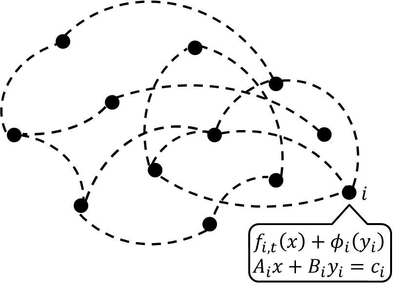
Figure 1: Distributed ADMM problem over a network; each agent operates based of the local objective $f_{i,t}(x)+\phi_{i}(y_{i})$ and the local linear constraint $A_{i}x+B_{i}y_{i}=c_{i}$.

The local decisions made by agent $i$ is represented by the optimization variables $x_{i}\in\mathcal{X}$ and $y_{i}\in Y$; note that we allow the agents to have a local (not necessary exact) version of the global variable $x$, namely $x_{i}$. In addition, we assume that subgradients $\partial f_{i,t}(x)$ can be computed for every $x\in\chi$. In the online setting, based on the available local information, each decision maker $i$ selects a global variable $x_{i,t}\in\chi$ and local variable $y_{i,t}\in Y$, at time $t$. The cost $f_{i,t}(x_{i,t})$ is then revealed to this agent after its local decision $x_{i,t}$ has been committed to at time $t$.

III-A Regret for Constrained Optimization

We now examine a measure for evaluating the performance of OD-ADMM based on variational inequalities. measure is inspired by the convergence analysis of Douglas-Rachford ADMM presented in [24].

Consider the Lagrangian for the constrained optimization problem (9) as

$$\mathcal{L}_{T}(x,y,\lambda)=\sum_{t=1}^{T}\left\{f_{t}(x)+\frac{1}{n}\sum_{i=1}^{n}(\phi_{i}(y_{i})+\left\langle\lambda_{i},r_{i}(x,y_{i})\right\rangle)\right\},$$ (11)

where $x\in\mathcal{X}$ and $y_{i}\in Y$, as well as assuming $\lambda_{i}\in\mathbb{\mathbb{R}}^{m_{i}}$, for all $i\in\left[n\right]$. Then, the Lagrange dual function is defined as

$$\mathcal{D}(\lambda)=\inf_{x\in\chi,y_{i}\in Y}\mathcal{L}_{T}(x,y,\lambda),$$ (12)

implying that $\mathcal{D}(\lambda)$ is concave and yields a lower bound on the optimal value of (9) [9]. Hence, the dual function $D(\lambda)$ is maximized with respect to the variable $\lambda\in\mathbb{\mathbb{R}}^{m_{i}\times n}$,

$$\mathcal{D}^{*}=\max_{\lambda\in\mathcal{Z}^{n}}\mathcal{D}(\lambda)=\max_{\lambda\in\mathcal{Z}^{n}}\mathcal{L}_{T}(x^{*},y^{*},\lambda);$$ (13)

we note that $\mathcal{Z}^{n}\subseteq\mathbb{\mathbb{R}}^{m_{i}\times n}$. Slater condition guarantees zero duality gap and the existence of a dual optimal solution $\lambda^{*}\in\mathcal{Z}^{n}$. When $(x^{*},y_{1}^{*},\cdots,y_{n}^{*})\in\chi\times Y^{n}$ solves the primal problem (9)-(10), the primal and dual optimal vectors form a saddle-point for the Lagrangian $\mathcal{L}_{T}$ [25]. Thus, based on the saddle point theorem, if $w^{*}=(x^{*},y_{1}^{*},\cdots,y_{n}^{*},\lambda_{1}^{*},\cdots,\lambda_{n}^{*})\in\Omega$ is a saddle point for $\mathcal{L}_{T}$, then for all $w=(x,y_{1},\cdots,y_{n},\lambda_{1},\cdots,\lambda_{n})\in\chi\times Y^{n}\times\mathbb{\mathbb{R}}^{m_{i}\times n}=\Omega$, we have

$$\mathcal{L}_{T}(x^{*},y^{*},\lambda)\leq\mathcal{L}_{T}(x^{*},y^{*},\lambda^{*})\leq\mathcal{L}_{T}(x,y,\lambda^{*}).$$ (14)

Moreover, the Slater condition implies that the dual optimal set is bounded; hence $\left\|\lambda_{i}^{*}\right\|\leq D_{\lambda}$ for all $i\in[n]$ for some finite $D_{\lambda}$ (see Lemma 3 in [26]). A consequence of inequality (14) is that $\widetilde{w}=\left(\widetilde{x},\widetilde{y},\widetilde{\lambda}\right)\in\Omega$ approximately solves the primal problem with accuracy $\epsilon_{T}^{\mathcal{P}}\geq 0$ if it satisfies,

$$0\leq\mathcal{L}_{T}(\widetilde{x},\widetilde{y},\lambda^{*})-\mathcal{L}_{T}(x^{*},y^{*},\lambda^{*})\leq\epsilon_{T}^{\mathcal{P}},$$

that is,

$$0\leq\mathcal{L}_{T}(\widetilde{x},\widetilde{y},\lambda^{*})-\mathcal{P}^{*}\leq\epsilon_{T}^{\mathcal{P}}.$$ (15)

Based on (12), the inequality (15) can also be referred as dual feasibility. In addition, $\widetilde{w}=\left(\widetilde{x},\widetilde{y},\widetilde{\lambda}\right)\in\Omega$ approximately solves the dual problem with accuracy $\epsilon_{T}^{\mathcal{D}}\geq 0$ if

$$0\leq\mathcal{L}_{T}(x^{*},y^{*},\lambda^{*})-\mathcal{L}_{T}(x^{*},y^{*},\widetilde{\lambda})\leq\epsilon_{T}^{\mathcal{D}},$$

that is,

$$0\leq\mathcal{D}^{*}-\mathcal{D}(\widetilde{\lambda})\leq\epsilon_{T}^{\mathcal{D}},$$ (16)

which represents the dual sub-optimality. The conditions in (15)-(16) can be combined to represent the duality gap as

$$\sum_{t=1}^{T}f_{t}^{\Delta}(\widetilde{w},w^{*})+\frac{1}{n}(\sum_{i=1}^{n}\phi_{i}^{\Delta}(\widetilde{w},w^{*})+H_{i}^{\Delta}(\widetilde{w},w^{*}))\leq\epsilon_{T}.$$

where

$$f_{t}^{\Delta}(w,w^{*}) =f_{t}(x)-f_{t}(x^{*})$$

$$\phi_{i}^{\Delta}(w,w^{*}) =\phi_{i}(y_{i})-\phi_{i}(y_{i}^{*})$$

$$H_{i}^{\Delta}(w,w^{*}) =h_{1i}^{\Delta}(w,w^{*})+h_{2i}^{\Delta}(w,w^{*})$$

$$h_{1i}^{\Delta}(w,w^{*}) =\left\langle x-x^{*},A_{i}^{T}\lambda_{i}^{*}\right\rangle+\left\langle\lambda_{i}-\lambda_{i}^{*},-r_{i}(x^{*},y_{i}^{*})\right\rangle$$

$$h_{2i}^{\Delta}(w,w^{*}) =\left\langle y_{i}-y_{i}^{*},B_{i}^{T}\lambda_{i}^{*}\right\rangle,$$

and $\epsilon_{T}=\epsilon_{T}^{\mathcal{P}}+\epsilon_{T}^{\mathcal{D}}\geq 0$. This gap is illustrated in Figure 2.

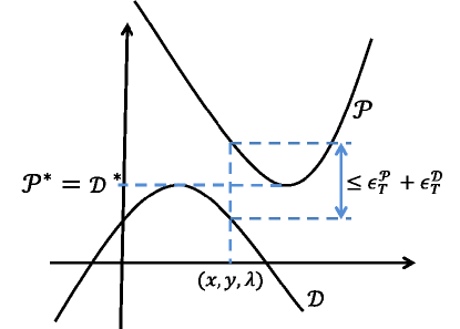
Figure 2: This figure illustrates the duality gap at $w=\left(x,y,\lambda\right)\in\Omega$.

Analogous to the regret definition for O-ADMM algorithm [27], we can consider a sequence of decisions $w_{t}$, where $w_{t}\in\Omega$ for each $t$, instead of a fixed decision $\widetilde{w}$. Consequently, the sequence $w_{t}$ approximately solves (9) and (10) with accuracy $\epsilon_{T}$ if

$$\sum_{t=1}^{T}f_{t}^{\Delta}(w_{t},w^{*})+\frac{1}{n}\left\{\sum_{i=1}^{n}\phi_{i}^{\Delta}(w_{t},w^{*})+H_{i}^{\Delta}(w_{t},w^{*})\right\}\leq\epsilon_{T},$$ (17)

for the optimal solution $w^{*}\in\Omega$, referred to as fixed case solutions to distinguish them from the time-varying online solution sequence $w_{t}$. Moreover, the mapping $H_{i}^{\Delta}(w,w^{*})$ can be expressed as

$$H_{i}^{\Delta}(w,w^{*})=\left\langle w_{i}(x)-w_{i}^{*}(x),H_{i}(w^{*})\right\rangle,$$

where $w_{i}(x)=\left[\begin{array}[]{ccc}x&y_{i}&\lambda_{i}\end{array}\right]^{T}$, $w_{i}^{*}(x)=\left[\begin{array}[]{ccc}x&y_{i}^{*}&\lambda_{i}^{*}\end{array}\right]^{T}$, and

$$H_{i}(w)=\left[\begin{array}[]{ccc}0&0&A_{i}^{T}\\ 0&0&B_{i}^{T}\\ -A_{i}&-B_{i}&0\end{array}\right]w_{i}(x)+\left[\begin{array}[]{c}0\\ 0\\ c_{i}\end{array}\right].$$

Since, the mapping $H_{i}(w)$ is affine in $w_{i}(x)$ and is defined through a skew symmetric matrix, it is monotone, and consequently [28]

$$\left\langle w_{i}(x)-w_{i}^{*}(x),H_{i}(w)-H_{i}(w^{*})\right\rangle\geq 0$$

$$\left\langle w_{i}(x)-w_{i}^{*}(x),H_{i}(w)\right\rangle\geq\left\langle w_{i}(x)-w_{i}^{*}(x),H_{i}(w^{*})\right\rangle.$$ (18)

Therefore, the inequality

$$\sum_{t=1}^{T}f_{t}^{\Delta}(w_{t},w^{*})+\frac{1}{n}\sum_{i=1}^{n}\left(\phi_{i}^{\Delta}(w_{t},w^{*})+\left\langle w_{i,t}(x)-w_{i}^{*}(x),H_{i}(w_{t})\right\rangle\right) \leq\epsilon_{T}$$ (19)

is a sufficient condition for (17).

Finally, motivated by the inclusion of regularization terms in the augmented Lagrangian method [25], the term on the left hand side of (19) is supplemented with terms of the form $\frac{\rho}{2}||r_{i}(x_{i,t},y_{i,t})||^{2}$, where $\rho>0$, to promote agents satisfy the local primal feasibility constraints. In our setting, the sequence $w_{i,t}$ is constructed from the distributed algorithm adopted by each agent $i$, specifically $w_{t}(x_{i,t})=(x_{j,t},y_{t},\lambda_{t+1})\in\Omega$ at time $t$, where $y_{t}=\left(y_{1,t},\cdots,y_{n,t}\right)$ and $\lambda_{t+1}=\left(\lambda_{1,t+1},\cdots,\lambda_{n,t+1}\right)$. The social regret is thus defined as,

$$R_{T}=\max_{j\in[n]}R_{j,T},$$

where

$$R_{j,T} =\sum_{t=1}^{T}f_{t}^{\Delta}(w_{t}(x_{j,t}),w^{*})+\frac{1}{n}\sum_{i=1}^{n}\left\{\phi_{i}^{\Delta}(w_{t}(x_{j,t}),w^{*})+\left\langle w_{i,t}(x_{j,t})-w_{i}^{*}(x_{j,t}),H_{i}(w_{t}(x_{j,t}))\right\rangle+\frac{\rho}{2}||r_{i}(x_{i,t},y_{i,t})||^{2}\right\}.$$ (20)

Based on (19) we say that the sequence $w_{i,t}$ approximately solves (9) and (10) with accuracy $\epsilon_{T}$ if it satisfies $R_{T}\leq\epsilon_{T}$. Therefore, if the social regret is sub-linear with time, the online algorithm performs as well as the best fixed case decision provided with the complete sequence of cost functions a priori. In addition, the sub-linearity of the social regret ensures that the local linear constraints will be satisfied asymptotically.

IV Main Result

The main contribution of this paper is extending O-ADMM [8] via Nesterov’s Dual Averaging (DA) algorithm [29] and distributed subgradients (descent) method discussed in [13, 30, 31, 32], to provide a distributed decision-making process for the optimization problem discussed in §III with a sub-linear social regret; we refer to this procedure as online distributed ADMM (OD-ADMM). The main challenge for the seamless integration of ADMM with dual averaging and distributed gradient descent for OD-ADMM is deriving and utilizing bounds on the network effect and the sub-optimality of the local decisions on the quality of the agent’s decisions on the social regret. This objective is achieved by building on the existing results reported in [13, 14, 15] regarding the network contribution in distributed optimization, as well as extensions of results discussed in [7, 8, 1]. basic idea behind our convergence analysis is as follows. First, in Lemmas 6 and 7, we derive the gap between the local decisions and the average decision over the network. Then, we provide the sub-optimality gap in Lemmas 8 and 9. Finally, building on previous results, bounds on the social regret are presented in Theorems 1 and 2.

The proposed algorithm updates the vector $(x_{i},y_{i},z_{i},\lambda_{i})$ for each agent $i\in[n]$ by alternately minimizing the Lagrangian and augmented Lagrangian. In addition, the Lagrangian is linearized based on network-level update, leading to a subgradient descent method followed by a projection step onto the constraint set $\chi$. Specifically, in the DA method, we let

$$z_{t+1}=z_{t}+\tilde{g}_{t},$$

where $\tilde{g}_{t}=\nabla\mathcal{L}_{t}(x_{t})$, followed by

$$x_{t+1}=\prod_{\chi}^{\psi}\left(z_{t+1},\alpha_{t}\right);$$ (21)

in this case, the parameter $\alpha_{t}$ is a non-increasing sequence of positive functions and $\prod_{\chi}^{\psi}(\cdot)$ is the projection operator onto $\chi$ defined as

$$\prod_{\chi}^{\psi}(z_{t+1},\alpha_{t})\equiv\arg\min_{x\in\chi}\left\{\left\langle z_{t+1},x\right\rangle+\frac{1}{\alpha_{t}}\psi(x)\right\};$$ (22)

the proximal function $\psi(x):\chi\rightarrow\mathbb{R}$ is continuously differentiable and strongly convex . The inclusion of the proximal function in the DA method as a regularizer prevents oscillations in the projection step. to be strongly convex with respect to $\|.\|$, $\psi\geq 0$, and $\psi(0)=0$.

On the other hand, in the subgradient descent (GD) method, the aforementioned steps in DA are replaced by

$$h_{t+1}=x_{t}-\alpha_{t}\tilde{g}_{t},$$

followed by

$$x_{t+1}=\prod_{\chi}h_{t+1}\equiv\arg\min_{x\in\chi}||x-h_{t+1}||.$$ (23)

Finally, the proposed online algorithm minimizes the augmented Lagrangian over $y$ as

$$y_{t+1}=\arg\min_{y\in Y}\left\{\mathcal{L}_{t}(x_{t+1},y,\lambda_{t+1})+\frac{\rho}{2}||r(x_{t+1},y)||^{2}\right\},$$

and update the dual variable $\lambda$ as

$$\lambda_{t+2}=\lambda_{t+1}+\rho(Ax_{t+1}+By_{t+1}-c).$$

The distributed algorithm can be considered as an approximate ADMM by an agent $i$ via a convex combination of information provided by its neighbors $N(i)$. Specifically, the global update step (21) and (23) can be reformulated with a distributed method. The underlying communication network can be represented compactly as a doubly stochastic matrix $P\in\mathbb{R}^{n\times n}$ which preserves the zero structure of the Laplacian matrix $L(\mathcal{G})$. For agents to have access to information contained in the subgradients $\tilde{g}_{i,t}=\nabla\mathcal{L}_{i,t}(x_{i,t})$ there must be information flow amongst the agents; as such, in our subsequent analysis it will be assumed that the graph $\mathcal{G}$ is strongly connected. A method to construct a doubly stochastic matrix $P$ of the required form from the Laplacian of the network is provided in Proposition 3.

The online distributed ADMM (OD-ADMM) is presented in Algorithm 1.

1Initialize $x_{i,1}=0$ and $y_{i,1}=0$ for all $i=1,...,n$

2 for $t=1$ to $T$ do

3       Adversary reveals $f_{t}(t)=\{f_{i,t}(t);\;\mbox{for}\;\forall i=1,...,n\}$

4       Compute subgradient $g_{i}(t)\in\partial f_{i,t}(x_{i,t})$

5       foreach Agent $i$ do

6             $\lambda_{i,t+1}=\lambda_{i,t}+\rho(A_{i}x_{i,t}+B_{i}y_{i,t}-c_{i})$ 

7            $x_{i,t+1}=H_{\alpha_{t}}(\lambda_{i,t+1},g_{i,t})$ 

8            $r_{i}(x_{i,t+1},y)=A_{i}x_{i,t+1}+B_{i}y-c_{i}$ 

9            $y_{i,t+1}=\mbox{argmin}_{y\in Y}\left\{\phi_{i}(y)+\lambda_{i,t+1}^{T}r_{i}(x_{i,t+1},y)+\frac{\rho}{2}||r_{i}(x_{i,t+1},y)||^{2}\right\}$ 

10      end

11end

Algorithm 1 Online Distributed ADMM (OD-ADMM)

The function $H_{\alpha_{t}}(\lambda_{i,t+1},g_{i,t})$ referred to on line 8 of the algorithm represents a distributed update on the primal variable. this paper, we consider two alternatives for this update.

IV-A OD-ADMM via Distributed Dual Averaging

In this method, the dual sub-gradient at each node is updated as a convex combination of its neighbor’s dual subgradients and itself, namely,

$$z_{i,t+1}=\sum_{j=1}^{n}P_{ji}z_{j,t}+g_{i,t}+A_{i}^{T}\lambda_{i,t+1},$$ (24)

and

$$x_{i,t+1}=\prod_{\chi}^{\psi}(z_{i,t+1},\alpha_{t}),$$ (25)

where the projection operator $\prod_{\chi}^{\psi}(\cdot)$ is defined in (22). Before presenting the convergence rate of the proposed OD-ADMM algorithm we provide a few preliminary remarks and definitions. Let us define the sequences of (network) average dual subgradients $z_{t}$’s and average subgradients $g_{t}$’s as

$$z_{t} =\frac{1}{n}\sum_{i=1}^{n}z_{i,t},\;\;\;g_{t}=\frac{1}{n}\sum_{i=1}^{n}g_{i,t}.$$ (26)

Thus, in the distributed DA method, the following update rule is introduced similar to the standard DA algorithm,

$$z_{t+1}=z_{t}+g_{t}+\frac{1}{n}\sum_{i=1}^{n}A_{i}^{T}\lambda_{i,t+1},$$ (27)

where the primal update is

$$\theta_{t+1}=\Pi_{\chi}^{\psi}(z_{t+1},\alpha_{t}).$$ (28)

The regret analysis can now be presented as follows, where the intermediate results required for its proof are relegated to the Appendix, namely Lemmas 5, 6, and 8. In particular, we show that with a proper choice of learning rate in Lemmas 6 and 8, the network effect and the sub-optimality of average decisions are sub-linear over time. Subsequently, building on these results, a sub-linear regret bound for OD-ADMM using distributed DA method can be established as formalized by the following result.

Theorem 1.

Given the sequence $w_{i,t}$ generated by Algorithm 1 where line 1 applies distributed dual-averaging method with $\psi(x^{*})\leq\Psi^{2}$ and $\alpha(t)=k/\sqrt{t}$, we have

$$R_{T}\leq J_{1}+J_{2}k\sqrt{T},$$ (29)

where

$$J_{1}=\frac{D_{\lambda}}{\rho n}\sum_{i=1}^{n}\frac{\mathcal{\zeta}_{i}}{\sigma_{1}(A_{i})},$$

$$J_{2} =2\mathcal{Q}(L_{f}+\zeta^{\max})(\frac{2}{n}\sum_{i}(D_{\lambda}\sigma_{1}(A_{i})+2\zeta_{i})),$$

with

$$\overline{\mathcal{\zeta}}=\frac{1}{n}\sum_{i=1}^{n}\mathcal{\zeta}_{i},\,\zeta^{\max}=\max_{i}\mathcal{\zeta}_{i},$$

$$\mathcal{\zeta}_{i}=\sqrt{m_{i}}L_{\phi}\frac{\sigma_{1}(A_{i})}{\sigma_{m_{i}}(B_{i}^{T})},\mbox{ and }\mathcal{Q}=\frac{\sqrt{n}}{1-\sigma_{2}(P)}.$$

Proof:

Based on the definition of $f_{t}$ we have

$$f_{t}^{\Delta}(w_{t}(x_{j,t}),w^{*})=\frac{1}{n}\sum_{i=1}^{n}f_{i,t}^{\Delta}(w_{t}(x_{j,t}),w^{*}),$$

where $w_{t}(x_{j,t})=(x_{j,t},y_{t},\lambda_{t+1})\in\Omega$ and thus

$$R_{j,T}=\frac{1}{n}\sum_{i,t}f_{i,t}^{\Delta}(w_{t}(x_{j,t}),w^{*})+\phi_{i}^{\Delta}(w_{t}(x_{j,t}),w^{*})+H_{i}^{\Delta}(w_{t}(x_{j,t}),w^{*})+\frac{\rho}{2}||r_{i}(x_{i,t},y_{i,t})||^{2}.$$

In the meantime as $f_{t}$ is $L$-Lipschitz and convex, we have

$$f_{t}^{\Delta}(w_{t}(x_{j,t}),w^{*}) =f_{t}(x_{j,t})-f_{t}(\theta_{t})+f_{t}(\theta_{t})-f_{t}(x^{*})$$

$$\leq L_{f}\left\|x_{j,t}-\theta_{t}\right\|+\left\langle g_{t},\theta_{t}-x^{*}\right\rangle.$$ (30)

The first term in (30) represents the network effect in the regret bound, i.e., the deviation of local primal variable at each node from the average primal variable. Lemma 6 in the Appendix on the other hand, provides a bound on the network effect using the DA method. Therefore, replacing line 1 of Algorithm 1 with the distributed DA method implies that

$$\|\theta_{t}-x_{j,t}\|\leq\alpha_{t-1}\frac{\sqrt{n}\,(L_{f}+\zeta^{\max})}{1-\sigma_{2}(P)}.$$ (31)

Moreover, from the integral test with $\alpha_{t}=k/\sqrt{t}$ it follows that

$$\sum_{t=1}^{T}\alpha_{t-1}\leq 2k\sqrt{T}.$$ (32)

Hence, from (31) and (32) it follows that

$$\sum_{t=1}^{T}\|x_{j,t}-\theta_{t}\|\leq 2k\sqrt{T}\mathcal{Q}(L_{f}+\zeta^{\max}).$$ (33)

The second term in (30) represents the sub-optimality of the procedure due to using the subgradient method. Applying Lemma 8 (Appendix) with (27) and (28) implies that

$$\sum_{t=1}^{T}\left\langle g_{t},\theta_{t}-x^{*}\right\rangle\leq\sum_{t=1}^{T}[\frac{\alpha_{t}}{2}\left\|\vphantom{g_{t+1}}\right.g_{t+1}+\frac{1}{n}\sum_{i=1}^{n}A_{i}^{T}\lambda_{i,t+2}\left.\vphantom{g_{t+1}}\right\|_{*}^{2}$$

$$\hphantom{\leq}\;\;\;\;\;\;\;\;\;\;\;\;\;\;\;\;\;\;\;\;\;\;+\frac{1}{n}\sum_{i=1}^{n}\left\langle\lambda_{i,t+1},A_{i}(x^{*}-\theta_{t})\right\rangle]+\frac{1}{\alpha_{T}}\psi\left(x^{*}\right).$$ (34)

The first term on the the right hand side of (34) represents the sub-optimality of Lagrangian function, defined in (11), with respect to the global variable $x$ and is bounded as

$$\sum_{t=1}^{T}\frac{\alpha_{t}}{2}\left\|\vphantom{g_{t+1}}\right.g_{t+1}+\frac{1}{n}\sum_{i=1}^{n}A_{i}^{T}\lambda_{i,t+2}\left.\vphantom{g_{t+1}}\right\|_{*}^{2}\leq(\max_{t}\left\|g_{t+1}\right\|_{*}+\frac{1}{n}\sum_{i=1}^{n}\sigma_{1}(A_{i})\max_{t}\left\|\lambda_{i,t}\right\|_{*})^{2}\sum_{t=1}^{T}\frac{\alpha_{t}}{2}.$$ (35)

We now proceed to bound the individual terms in (35). By optimality of line 1 in Algorithm 1 and applying line 1, we have

$$\nabla_{y}\phi_{i}(y_{i,t})=-B_{i}^{T}\left(\lambda_{i,t}+\rho r_{i}(x_{i,t},y_{i,t})\right)=-B_{i}^{T}\lambda_{i,t+1},$$

for all $i\in[n]$ and $t\in[T]$. Moreover, since $||\nabla_{y}\phi_{i}(y_{i,t})||\leq L_{\phi}$, we have $||B_{i}^{T}\lambda_{i,t+1}||\leq L_{\phi}$. Thus, $\lambda_{i,t}$ is bounded as

$$||\lambda_{i,t}|| \leq||(B_{i}B_{i}^{T})^{-1}B_{i}||_{F\;}||B_{i}^{T}\lambda_{i}||\leq L_{\phi}(\sum_{j=1}^{m_{i}}\frac{1}{\sigma_{j}^{2}(B_{i}^{T})})^{1/2}\leq\frac{\sqrt{m_{i}}L_{\phi}}{\sigma_{m_{i}}(B_{i}^{T})},$$ (36)

which implies that $||A_{i}^{T}\lambda_{i,t}||\leq\sqrt{m_{i}}L_{\phi}\sigma_{1}(A_{i})/\sigma_{m_{i}}(B_{i}^{T}).$ Based on Lipschitz continuity of $f_{t}$, we have that $\left\|g_{t+1}\right\|_{*}\leq L_{f},$ and subsequently (35) is bounded as

$$\sum_{t=1}^{T}\frac{\alpha_{t}}{2}\left\|\vphantom{g_{t+1}}\right.g_{t+1}+\frac{1}{n}\sum_{i=1}^{n}A_{i}^{T}\lambda_{i,t+2}\left.\vphantom{g_{t+1}}\right\|_{*}^{2}\leq(L_{f}+\overline{\mathcal{\zeta}})^{2}k\sqrt{T}.$$ (37)

The second term in the inequality (34) represents the sub-optimality of centralized decision $\theta$ with respect to the linear constraints. In order to analyze this term, it is first expanded into two terms representing the sub-optimality of local decision $x_{i,t}$ and the network effect, respectively, i.e.,

$$\left\langle\lambda_{i,t+1},A_{i}(x^{*}-\theta_{t})\right\rangle$$

$$=\left\langle\lambda_{i,t+1},A_{i}(x^{*}-x_{j,t})\right\rangle+\left\langle\lambda_{i,t+1},A_{i}(x_{j,t}-\theta_{t})\right\rangle$$

$$=\left\langle\lambda_{i,t+1},A_{i}(x^{*}-x_{j,t})\right\rangle+\left\langle\lambda_{i}^{*}-\lambda_{i,t+1},-r_{i}(x_{j,t},y_{i,t})\right\rangle$$

$$\;\;\;\;+\left\langle\lambda_{i,t+1},A_{i}(x_{j,t}-\theta_{t})\right\rangle+\left\langle\lambda_{i}^{*}-\lambda_{i,t+1},r_{i}(x_{j,t},y_{i,t})\right\rangle$$

$$=-h_{1i}^{\Delta}(w_{t}(x_{j,t}),w^{*})+\left\langle\lambda_{i,t+1},A_{i}(x_{j,t}-\theta_{t})\right\rangle+\left\langle\lambda_{i}^{*}-\lambda_{i,t+1},r_{i}(x_{j,t},y_{i,t})\right\rangle.$$ (38)

Based on the network effect introduced in (31), we have

$$\left\langle\lambda_{i,t+1},A_{i}(x_{j,t}-\theta_{t})\right\rangle\leq\sigma_{1}(A_{i})||\lambda_{i,t+1}||\;\|x_{j,t}-\theta_{t}\|.$$ (39)

Moreover, applying (33) and (36) to (39), it follows that

$$\sum_{t=1}^{T}\left\langle\lambda_{i,t+1},A_{i}(x_{j,t}-\theta_{t})\right\rangle\leq 2k\sqrt{T}\mathcal{\zeta}_{i}\mathcal{Q}(L_{f}+\zeta^{\max}).$$ (40)

The final term in (38) represents the first order necessary condition for optimality of the dual problem at $\lambda_{i,t+1}$. By applying line 7 of the algorithm and an inner product equality, we obtain

$$\left\langle\lambda_{i}^{*}-\lambda_{i,t+1},r_{i}(x_{j,t},y_{i,t})\right\rangle =\frac{1}{\rho}\left\langle\lambda_{i}^{*}-\lambda_{i,t+1},\lambda_{i,t+1}-\lambda_{i,t}\right\rangle+\left\langle\lambda_{i}^{*}-\lambda_{i,t+1},A_{i}(x_{j,t}-x_{i,t})\right\rangle$$

$$=\frac{1}{2\rho}(-\left\|\lambda_{i,t+1}-\lambda_{i,t}\right\|^{2}+\left\|\lambda_{i}^{*}-\lambda_{i,t}\right\|^{2}-\left\|\lambda_{i}^{*}-\lambda_{i,t+1}\right\|^{2})$$

$$\;\;\;\;+\left\langle\lambda_{i}^{*}-\lambda_{i,t+1},A_{i}(x_{j,t}-x_{i,t})\right\rangle$$

$$=\frac{1}{2\rho}(\left\|\lambda_{i}^{*}-\lambda_{i,t}\right\|^{2}-\left\|\lambda_{i}^{*}-\lambda_{i,t+1}\right\|^{2})-\frac{\rho}{2}\left\|r_{i}(x_{i,t},y_{i,t})\right\|^{2}$$

$$\;\;\;\;+\left\langle\lambda_{i}^{*}-\lambda_{i,t+1},A_{i}(x_{j,t}-x_{i,t})\right\rangle.$$ (41)

Resolving the telescoping sum

$$\sum_{t=1}^{T}\left\|\lambda_{i}^{*}-\lambda_{i,t}\right\|^{2}-\left\|\lambda_{i}^{*}-\lambda_{i,t+1}\right\|^{2},$$

using the fact $\lambda_{i,1}=0$, it now follows that

$$\sum_{t=1}^{T}\left\langle\lambda_{i}^{*}-\lambda_{i,t+1},r_{i}(x_{i,t},y_{i,t})\right\rangle \leq\frac{1}{2\rho}(\left\|\lambda_{i}^{*}\right\|^{2}-\left\|\lambda_{i}^{*}-\lambda_{i,T+1}\right\|^{2})-\frac{\rho}{2}\sum_{t=1}^{T}\left\|r_{i}(x_{i,t},y_{i,t})\right\|^{2}$$

$$\leq\frac{1}{2\rho}(2\left\|\lambda_{i}^{*}\right\|\left\|\lambda_{i,T+1}\right\|)-\frac{\rho}{2}\sum_{t=1}^{T}\left\|r_{i}(x_{i,t},y_{i,t})\right\|^{2}.$$

Applying (36) in conjunction with the assumption $\left\|\lambda_{i}^{*}\right\|\leq D_{\lambda}$,

$$\sum_{t=1}^{T}\left\langle\lambda_{i}^{*}-\lambda_{i,t+1},r_{i}(x_{i,t},y_{i,t})\right\rangle\leq\frac{D_{\lambda}\mathcal{\zeta}_{i}}{\rho\sigma_{1}(A_{i})}-\frac{\rho}{2}\sum_{t=1}^{T}\left\|r_{i}(x_{i,t},y_{i,t})\right\|^{2}.$$ (42)

The last term in (41) can also be bounded as

$$\left\langle\lambda_{i}^{*}-\lambda_{i,t+1},A_{i}(x_{j,t}-x_{i,t})\right\rangle \leq(D_{\lambda}\sigma_{1}(A_{i})+\zeta_{i})\|x_{j,t}-\theta_{t}\|\|x_{i,t}-\theta_{t}\|$$

$$\leq 2\alpha_{t-1}\mathcal{Q}(L_{f}+\zeta^{\max})(D_{\lambda}\sigma_{1}(A_{i})+\zeta_{i})$$ (43)

Substituting (40), (42), and (43) into (38),

$$\frac{1}{n}\sum_{i=1}^{n}\sum_{t=1}^{T}\left\langle\lambda_{i,t+1},A_{i}\left(x^{*}-\theta_{t}\right)\right\rangle\leq J_{1}-\frac{1}{n}\sum_{i,t}\left\{h_{1i}^{\Delta}(w_{t}(x_{j,t}),w^{*})+\frac{\rho}{2}||r_{i}(x_{i,t},y_{i,t})||^{2}\right\}$$

$$+4k\sqrt{T}\mathcal{Q}(L_{f}+\zeta^{\max})(\frac{1}{n}\sum_{i=1}^{n}D_{\lambda}\sigma_{1}(A_{i})+\overline{\mathcal{\mathcal{\zeta}}}).$$ (44)

Applying $\psi\left(x^{*}\right)\leq\Psi^{2}$, $\alpha_{T}=k/\sqrt{T}$, and substituting (37), (44) into (34) and simplifying, the sub-optimality of the primal problem at the global decision $\theta_{t}$ can now be represented as

$$\sum_{t=1}^{T}\left\langle g_{t},\theta_{t}-x^{*}\right\rangle\leq J_{1}-\frac{1}{n}\sum_{i,t}\left\{h_{1i}^{\Delta}(w_{t}(x_{j,t}),w^{*})+\frac{\rho}{2}||r_{i}(x_{i,t},y_{i,t})||^{2}\right\}$$

$$+k\sqrt{T}\times(2\mathcal{Q}(L_{f}+\zeta^{\max})(\frac{2}{n}\sum_{i}(D_{\lambda}\sigma_{1}(A_{i})+2\zeta_{i})).$$ (45)

Based on our assumption of convexity of $\phi_{i}(\cdot)$, we have

$$\phi_{i}^{\Delta}(w_{i,t},w^{*}) \leq\left\langle\nabla_{y}\phi_{i}(y_{i,t}),y_{i,t}-y_{i}^{*}\right\rangle$$

$$\leq-\left\langle B_{i}^{T}\lambda_{i,t+1},y_{i,t}-y_{i}^{*}\right\rangle$$

$$=-h_{2i}^{\Delta}(w_{t}(x_{j,t}),w^{*}).$$ (46)

Combining (45) and (33) into (30) and adding (46), the regret can thereby be bounded as

$$R_{j,T}\leq J_{1}+J_{2}k\sqrt{T}$$

for all $j\in[n]$ and thus the social regret is bounded as $R_{T}\leq J_{1}+J_{2}k\sqrt{T}$. Note that the social regret represents the worst case regret amongst the agents in the network. ∎

The above theorem validates the “good” performance of OD-ADMM via dual averaging by demonstrating a sub-linear social regret. In addition, this social regret highlights the importance of the underlying interaction topology through $\sigma_{2}(P)$ and certain condition measure of local linear constraints through $\sigma_{1}(A_{i})$ and $\sigma_{m_{i}}(B_{i})$. A well known measure of network connectivity is the second smallest eigenvalue of the graph Laplacian $L(\mathcal{G})$ denoted by $\Lambda_{2}(\mathcal{G})$. Since the communication matrix $P$ is formed as proposed in Proposition 3, $1-\sigma_{2}(P)$ is proportional to $\Lambda_{2}(\mathcal{G})$ implying that high network connectivity promotes good performance of the proposed OD-ADMM algorithm with the embedded distributed implementation of dual averaging.

IV-B OD-ADMM via Distributed Gradient Descent

In this section, the local primal variable is updated using distributed GD method. In this method $x_{i,t}$ is updated as a convex combination of its neighbor’s local primal variables and itself, moving in the direction of decreasing the Lagrangian function,

$$h_{i,t+1}=\sum_{j=1}^{n}P_{ji}x_{j,t}-\alpha_{t}(g_{i,t}+A_{i}^{T}\lambda_{i,t+1}),$$ (47)

followed by the projection onto the convex set $\chi$,

$$x_{i,t+1}=\prod_{\chi}h_{i,t+1}.$$ (48)

In the distributed GD method, we first define the (network) average primal variable as

$$\theta_{t}=\frac{1}{n}\sum_{i=1}^{n}x_{i,t}.$$ (49)

The regret analysis for the OD-ADMM via the GD method can now be presented as follows, where the intermediate results required for its proof are relegated to the Appendix, namely Proposition 4, and Lemmas 7 and 9. In particular, with a proper choice of the learning rate in Lemmas 7 and 9, we can show that the network effect and sub-optimality of the average decision are sub-linear over time. Then, building on these results, a sub-linear social regret bound for OD-ADMM using distributed GD method can be obtained; this is formalized in the following theorem.

Theorem 2.

Given the sequence $w_{i,t}$ generated by Algorithm 1, where line 1 applies the distributed GD method with $\alpha(t)=k/\sqrt{t}$, we have

$$R_{T}\leq J_{1}+J_{2}k\sqrt{T},$$ (50)

where

$$J_{1}=\frac{D_{\lambda}}{\rho n}\sum_{i=1}^{n}\frac{\mathcal{\zeta}_{i}}{\sigma_{1}(A_{i})}+\frac{D_{\chi}^{2}}{2k},$$

$$J_{2} =4\mathcal{Q}(L_{f}+\zeta^{\max})(\frac{1}{n}\sum_{i=1}^{n}D_{\lambda}\sigma_{1}(A_{i})+2\overline{\mathcal{\zeta}})+2(L_{f}+\overline{\mathcal{\zeta}})^{2}+8L_{f}\mathcal{Q}(L_{f}+\overline{\mathcal{\zeta}}),$$

with

$$\overline{\mathcal{\zeta}}=\frac{1}{n}\sum_{i=1}^{n}\mathcal{\zeta}_{i},\,\zeta^{\max}=\max_{i}\mathcal{\zeta}_{i},$$

$$\mathcal{\zeta}_{i}=\sqrt{m_{i}}L_{\phi}\frac{\sigma_{1}(A_{i})}{\sigma_{m_{i}}(B_{i}^{T})},\mbox{ and }\mathcal{Q}=\frac{\sqrt{n}}{1-\sigma_{2}(P)}.$$

Proof:

Based on the definition of $f_{t}$ we have

$$f_{t}^{\Delta}(w_{t}(x_{j,t}),w^{*})=\frac{1}{n}\sum_{i=1}^{n}f_{i,t}^{\Delta}(w_{t}(x_{j,t}),w^{*}),$$

where $w_{t}(x_{j,t})=(x_{j,t},y_{t},\lambda_{t+1})\in\Omega$ and thus

$$R_{j,T}=\frac{1}{n}\sum_{i,t}f_{i,t}^{\Delta}(w_{t}(x_{j,t}),w^{*})+\phi_{i}^{\Delta}(w_{t}(x_{j,t}),w^{*})+H_{i}^{\Delta}(w_{t}(x_{j,t}),w^{*})+\frac{\rho}{2}||r_{i}(x_{i,t},y_{i,t})||^{2}.$$

As $f_{t}$ is $L$-Lipschitz and convex, we have

$$f_{t}^{\Delta}(w_{t}(x_{j,t}),w^{*}) =f_{t}(x_{j,t})-f_{t}(\theta_{t})+f_{t}(\theta_{t})-f_{t}(x^{*})$$

$$\leq L_{f}\left\|x_{j,t}-\theta_{t}\right\|+\left\langle g_{t},\theta_{t}-x^{*}\right\rangle.$$ (51)

The first term in (51) represents the network effect in the regret bound, i.e., the deviation of local primal variable at each node from the average primal variable. In the meantime, Lemmas 6 and 7 in the Appendix provide bounds on the network effect when the DA and GD methods are used in line 1 of Algorithm 1, respectively. Therefore, replacing line 1 of Algorithm 1 with the distributed DA method implies

$$\|\theta_{t}-x_{j,t}\|\leq\alpha_{t-1}\frac{\sqrt{n}(L_{f}+\zeta^{\max})}{1-\sigma_{2}(P)},$$ (52)

and with the distributed GD,

$$\|\theta_{t}-x_{j,t}\|\leq 2\sqrt{n}(L_{f}+\zeta^{\max})\sum_{k=1}^{t-1}\alpha_{t-k}\sigma_{2}(P)^{k-1}.$$ (53)

Moreover, from (52) (and (32)) it follows that

$$\sum_{t=1}^{T}\|x_{j,t}-\theta_{t}\|\leq 4k\sqrt{T}(\mathcal{Q}(L_{f}+\zeta^{\max}).$$ (54)

Note that the upper bound in (54) is more conservative than the distributed DA method by a factor of $2$.

The second term in (51) represents the sub-optimality due to using sub-gradient method. Applying Lemma 9 with (47)- (49) then leads to

$$\sum_{t=1}^{T}\left\langle g_{t},\theta_{t}-x^{*}\right\rangle \leq\frac{2}{n^{2}}\sum_{t=1}^{T}\alpha_{t}(\sum_{i=1}^{n}||g_{i,t}+A_{j}^{T}\lambda_{i,t+1}||)^{2}+\sum_{t=1}^{T}(4L_{f}\sum_{k=0}^{t-1}\alpha_{t-k}\sigma_{2}(P)^{k})\frac{1}{n}\sum_{i=1}^{n}||(g_{i,t}+A_{i}^{T}\lambda_{i,t+1}||$$

$$+\frac{1}{n}\sum_{t=1}^{T}\sum_{i=1}^{n}\left\langle A_{i}^{T}\lambda_{i,t+1},x^{*}-\theta_{t}\right\rangle+\frac{1}{2\alpha_{1}}D_{\chi}^{2}.$$ (55)

The first term on the right hand side of (55) is bounded as

$$\frac{2}{n^{2}}\sum_{t=1}^{T}\alpha_{t}(\sum_{i=1}^{n}||g_{i,t}+A_{i}^{T}\lambda_{i,t+1}||)^{2}$$

$$\leq 2(\frac{1}{n}\sum_{i=1}^{n}\max_{t}\left\|g_{t+1}\right\|+\frac{1}{n}\sum_{i=1}^{n}\sigma_{1}(A_{i})\max_{t}\left\|\lambda_{i,t}\right\|)^{2}\sum_{t=1}^{T}\sum_{t=1}^{T}\alpha_{t}$$

$$\leq 2(L_{f}+\overline{\mathcal{\zeta}})^{2}k\sqrt{T}.$$ (56)

Similarly, the second term on the right hand side of (55) is bounded as

$$\sum_{t=1}^{T}(4L_{f}\sum_{k=0}^{t-1}\alpha_{t-k}\sigma_{2}(P)^{k})\frac{1}{n}\sum_{i=1}^{n}||(g_{i,t}+A_{i}^{T}\lambda_{i,t+1}||$$

$$\leq 8L_{f}k\sqrt{T}\mathcal{Q}(L_{f}+\overline{\mathcal{\zeta}}).$$ (57)

We now proceed to bound the third term in (55) and from (38) we have

$$\left\langle\lambda_{i,t+1},A_{i}(x^{*}-\theta_{t})\right\rangle =-h_{1i}^{\Delta}(w_{t}(x_{j,t}),w^{*})+\left\langle\lambda_{i,t+1},A_{i}(x_{j,t}-\theta_{t})\right\rangle+\left\langle\lambda_{i}^{*}-\lambda_{i,t+1},r_{i}(x_{j,t},y_{i,t})\right\rangle.$$ (58)

Analogous to the proof of Theorem 1, the second term of (58) is bounded as

$$\sum_{t=1}^{T}\left\langle\lambda_{i,t+1},A_{i}(x_{j,t}-\theta_{t})\right\rangle\leq 4k\sqrt{T}\mathcal{\zeta}_{i}\mathcal{Q}(L_{f}+\zeta^{\max}).$$ (59)

Based on (42) and (43), we have

$$\sum_{t=1}^{T}\left\langle\lambda_{i}^{*}-\lambda_{i,t+1},r_{i}(x_{j,t},y_{i,t})\right\rangle\leq\frac{D_{\lambda}\mathcal{\zeta}_{i}}{\rho\sigma_{1}(A_{i})}-\frac{\rho}{2}\sum_{t=1}^{T}\left\|r_{i}(x_{i,t},y_{i,t})\right\|^{2}+4k\sqrt{T}\mathcal{Q}(L_{f}+\zeta^{\max})(D_{\lambda}\sigma_{1}(A_{i})+\zeta_{i}).$$ (60)

Substituting (59) and (60) into (58),

$$\frac{1}{n}\sum_{i=1}^{n}\sum_{t=1}^{T}\left\langle\lambda_{i,t+1},A_{i}\left(x^{*}-\theta_{t}\right)\right\rangle\leq -\frac{1}{n}\sum_{i,t}[h_{1i}^{\Delta}(w_{t}(x_{j,t}),w^{*})+\frac{\rho}{2}||r_{i}(x_{i,t},y_{i,t})||^{2}]$$

$$+4k\sqrt{T}\mathcal{Q}(L_{f}+\zeta^{\max})(\frac{1}{n}\sum_{i=1}^{n}D_{\lambda}\sigma_{1}(A_{i})+2\overline{\mathcal{\zeta}})+\frac{D_{\lambda}}{\rho n}\sum_{i=1}^{n}\frac{\mathcal{\zeta}_{i}}{\sigma_{1}(A_{i})}.$$ (61)

From (56), (57), and (61), the bound on (55) for $\alpha_{t}=k/\sqrt{t}$ is simplified to

$$\sum_{t=1}^{T}\sum_{t=1}^{T}\left\langle g_{t},\theta_{t}-x^{*}\right\rangle\leq J_{1}-\frac{1}{n}\sum_{i,t}[h_{1i}^{\Delta}(w_{t}(x_{j,t}),w^{*})+\frac{\rho}{2}||r_{i}(x_{i,t},y_{i,t})||^{2}]$$

$$+2k\sqrt{T}(\mathcal{Q}(L_{f}+\zeta^{\max})(\frac{2}{n}\sum_{i=1}^{n}D_{\lambda}\sigma_{1}(A_{i})+4\overline{\mathcal{\zeta}})+(L_{f}+\overline{\mathcal{\zeta}})^{2}+4L_{f}\mathcal{Q}(L_{f}+\overline{\mathcal{\zeta}})).$$ (62)

In the meantime, based on the convexity of $\phi_{i}$,

$$\phi_{i}^{\Delta}(w_{t},w^{*}) \leq-h_{2i}^{\Delta}(w_{t}(x_{j,t}),w^{*}).$$ (63)

Combining (62) and (54) into (51) and adding (63) we obtain,

$$R_{j,T}\leq J_{1}+J_{2}k\sqrt{T}.$$

for all $j\in[n]$ and thus $R_{T}\leq J_{1}+J_{2}k\sqrt{T}$. ∎

Theorems 1 and 2 and their proofs provide a basis for comparing two effective methods for evaluating OD-ADMM. The bounds provided in (33) and (54) for the distributed DA and GD, respectively, although conservative, hint at the fact that in the distributed DA, the local copies of the global variable $x\in\chi$ might converge faster to consensus in the worst case scenario. Moreover, as discussed in the introduction, the distributed DA approach does not require sharing the primal variables $x_{i,t}$ amongst the agents, preserving their privacy during the distributed decision making process; this feature of the DA approach however is not shared by embedding the distributed GD in OD-ADMM.

V Example - Formation Acquisition with Points of Interest and Boundary Constraints

In order to demonstrate the applicability of the developed OD-ADMM, we consider the following problem from the area of distributed robotics. This so-called formation acquisition problem is as follows. Consider $n$ planar robots (agents) where the position of agent $i$, denoted as $y_{i}$, is restricted to the convex set $Y=\left[-1,1\right]^{2}$. The centroid of the formation is denoted by $x\in\mathbb{R}^{2}$ and similarly constrained to $\mathcal{X}=Y$. The formation shape is defined for each agent by its offset $c_{i}$ from the centroid, namely $x-y_{i}=c_{i}$. There is a known boundary $S$ which agents are required to avoid by increasing the distance to the boundary $\mbox{dist}(y_{i},S)=\inf_{x\in S}\left\|x-y_{i}\right\|$. This is achieved with a penalty function $\phi_{i}(y_{i})=\left(\mbox{dist}(y_{i},S)+1\right)^{-1}$ associated with agent $y_{i}$’s proximity to $S$. We note that when $\mbox{int}\left(S\bigcap\mathcal{X}\right)$ is the empty set, $\phi_{i}(y_{i})$ is convex.

At each time step $t$, agent $i$ obtains a location of interest $q_{i,t}$ and the centroid is ideally located close to these locations of interest promoted through the minimization of the function $f_{i,t}(x)=\frac{1}{2}\left\|x-q_{i,t}\right\|_{2}^{2}$. The example illustrated in Figure 3 takes the form of problem (9), namely

$$\min_{x\in\mathcal{X},y_{1},\dots y_{n}\in Y} \sum_{t=1}^{T}\sum_{i=1}^{n}(f_{i,t}(x)+\phi_{i}(y_{i}))$$

s.t. $$A_{i}x+B_{i}y_{i}=c_{i}\,\mbox{for all }i\in\left[n\right],$$

where $A_{i}=-B_{i}=I_{2}$ for all $i\in\left[n\right]$.

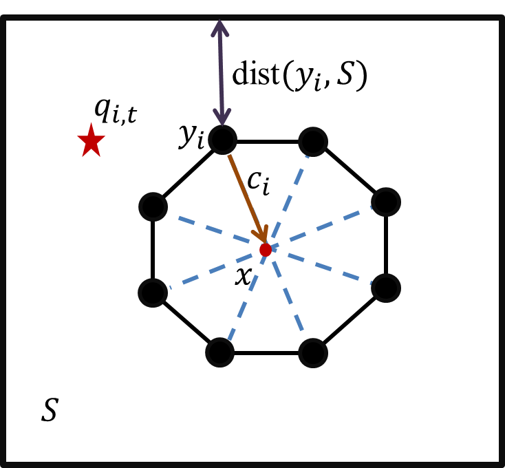
Figure 3: Formation acquisition problem amongst six planar robots or agents.

Consider $S=\left\{\left(x,y\right)\in\mathbb{R}|\left|x\right|=1.5,\left|y\right|=1.5\right\}$ and so $\phi_{i}(y_{i})=\left(2.5-\left\|y_{i}\right\|_{\infty}\right)^{-1}$. The relevant parameters of the ADMM algorithm are $g_{i}(t)=\nabla f_{i,t}(x_{i})=x_{i}-q_{i,t}$, $k=2,$ $\rho=0.5$, and $\psi(x)=\left\|x\right\|_{2}^{2}$. The remaining terms of the regret bound are $L_{\phi}=4/9$, $L_{f}=\sqrt{2}$, $\sigma_{1}(A_{i})=\sigma_{m_{i}}(B_{i})=1$, $D_{\lambda}=2$, and $K=1$.

The algorithm was applied to $n=8$ agents connected over a random graph (see Figure 5) with $\sigma_{2}(P)=0.78$ with $c_{i}$’s selected to acquire a formation with $n$ agents equidistant apart on the circumference of a circle of radius 0.4. Locations of interest switch at each time step between a uniform distribution over the area of a length 0.5 square centered at $\left(-0.75,0\right)$ and a Gaussian distribution with mean $\left(0,-0.75\right)$ and standard deviation $0.01I_{2}$, with bounds outside of $\mathcal{X}$ ignored. The convergence of the global variables $x_{i,t}$ to agreement as well as the reduction of the residue over time are displayed in Figure 4. Note that the local copies of the global variable converge faster to consensus using the distributed DA as compared with embedding the distributed GD for OD-ADMM.

The performance of the algorithm was compared for different graph topologies, namely path, star, cycle, random, cube and complete graphs. These graph topologies are displayed in Figure 5. The matrix $P$ was formed as proposed in Proposition 3, with $\epsilon=d_{\max}+1$, as such $\sigma_{2}(P)=1-\frac{1}{\epsilon}\Lambda_{2}(L(\mathcal{G})).$ Under the same locations of interest as described previously, the performance of the regret per time $R_{T}/T$ for each graph topology is compared in Figure 6. The performance strongly correlates with $\sigma_{2}(P)$, as predicted in Theorem 2, with smaller $\sigma_{2}(P)$ exhibiting improved performance.

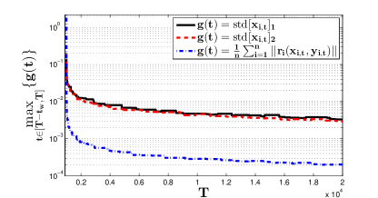
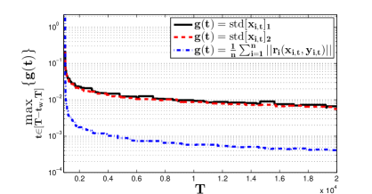
(a) Distributed Dual Averaging

(b) Distributed Gradient Descent

Figure 4: The standard deviation of the global variable $x_{i}$ and the average residue for each agent over times smoothed by taking the maximum over a $t_{w}=1000$ sliding window.

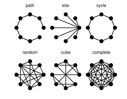
Figure 5: Topologies of the six different graph types considered for the formation acquisition problem.

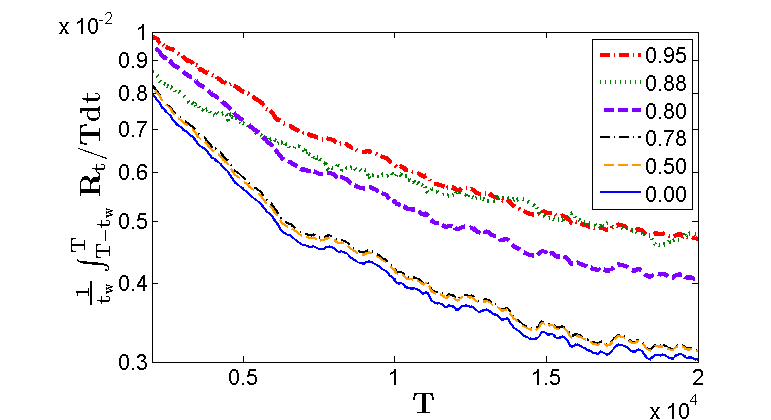
Figure 6: The social regret per time $R_{T}/T$ performance of six different graph types, specifically a path, star, cycle, random, cube and complete graph with $\sigma_{2}(P)$ of $0.95,0.88,0.80,0.78,0.50,0.00$, respectively. The trajectories are smoothed by taking the average over a $t_{w}=1000$ sliding window.

VI Conclusion

In this work, online distributed ADMM has been introduced and analyzed, where a network of decision-makers or agents cooperatively optimize an objective that decomposes to global and local objectives, and is partially online. Moreover, the local variables and the global variable are linearly constraint (specific to each agent). This problem setup has a wide range of applications in networked systems, such as in distributed robotics and computer networks. A distributed algorithm allows us to make decisions across the network based on local data and information exchange with neighboring agents.

The online distributed algorithm developed in this paper, achieves a sub-linear social regret of $O(\sqrt{T})$, that simultaneously captures sub-optimality of the objective function and the violations in the linear local constraints. In particular, this algorithm is competitive with respect to the best fixed decision performance in hindsight. Moreover, we have highlighted the role of the underlying network topology in achieving a “good” social regret, i.e., the regret bound improves with increased connectivity in the network. The proposed algorithm was then applied to a formation acquisition problem.

Future work of particular interest includes exploring social regret over a time varying network, and investigating favorable network characteristics for the proposed online distributed ADMM algorithm.

VII Appendix

The following results can be found in [14, 15, 33]; as such they are presented here with no or abridged proofs.

Proposition 3.

If graph $\mathcal{G}$ is strongly connected then the matrix $P=I-\frac{1}{\epsilon}\mbox{diag}\left(v\right)L(\mathcal{G})$ is doubly stochastic, where $v^{T}L\left(\mathcal{G}\right)=0$ with positive vector $v=\left[v_{1},v_{2},\dots,v_{n}\right]^{T}$ and $\epsilon\in(\max_{i\in V}(v_{i}d_{i}),\infty)$. If graph $\mathcal{G}$ is balanced then the matrix $P=I-\frac{1}{\epsilon}L(\mathcal{G})$ is doubly stochastic, where $\epsilon\in(d_{\max},\mbox{$\infty$})$.

Proposition 4.

For any $u\in\mathbb{R}^{m}$, $v\in\chi$, and orthogonal projection operator $\prod_{\chi}$ onto $\chi$ we have

$$\left\langle u-\prod_{\chi}(u),u-v\right\rangle\geq 0.$$

Lemma 5.

For any $u,v\in\mathbb{R}^{m}$, and under the conditions stated for the proximal function $\psi$ and step size $\alpha,$ we have

$$\|\prod_{\chi}^{\psi}(u,\alpha)-\prod_{\chi}^{\psi}(v,\alpha)\|\leq\alpha\|u-v\|_{*}.$$

Lemma 6.

For sequences $z_{i,t}$ and $x_{i,t}$ generated by Algorithm 1, using the distributed DA method where,

$$z_{i,t+1}=\sum_{j=1}^{n}P_{ji}z_{j,t}+g_{i,t}+A_{i}^{T}\lambda_{i,t+1}$$

and $x_{i,t+1}=\prod_{\chi}^{\psi}(z_{i,t+1},\alpha_{t})$, we have

$$\|\theta_{t}-x_{i,t}\|_{*} \leq\alpha_{t-1}\frac{\sqrt{n}(L_{f}+\zeta^{\max})}{1-\sigma_{2}(P)}$$

for all $i\in[n]$ and $t\in[T]$, where the sequence $\theta_{t}$ is generated by (28), $\mathcal{\zeta}_{i}=L_{\phi}{\sigma_{1}(A_{i})/\sigma_{1}(B_{i})}$, and $\zeta^{\max}=\max_{i}\mathcal{\mathcal{\zeta}}_{i}$.

Proof:

Based on the definition of $z_{i,t}$ we have

$$z_{i,t} =\sum_{j=1}^{n}\left[P^{t-1}\right]_{ji}z_{j,1}+\sum_{k=1}^{t-1}\sum_{j=1}^{n}\left[P^{k-1}\right]_{ji}\left(g_{j,t-k}+A_{j}^{T}\lambda_{j,t-k+1}\right).$$

In addition, $z_{t}$ evolves as

$$z_{t} =z_{1}+\sum_{k=1}^{t-1}\sum_{j=1}^{n}\frac{1}{n}(g_{j,t-k}+A_{j}^{T}\lambda_{j,t-k+1}).$$ (64)

Assuming $z_{i,1}=0$ for all $i\in[n]$ and based on (64) we have

$$z_{t}-z_{i,t} =\sum_{k=1}^{t-1}\sum_{j=1}^{n}(\frac{1}{n}-\left[P^{k-1}\right]_{ji})(g_{j,t-k}+A_{j}^{T}\lambda_{j,t-k+1})$$ (65)

Thus, the dual norm of $z_{t}-z_{i,t}$ can be bounded as

$$\|z_{t}-z_{i,t}\|_{*} \leq\sum_{k=1}^{t-1}\sum_{j=1}^{n}\left\|g_{j,t-k}+A_{j}^{T}\lambda_{j,t-k+1}\right\|_{*}|\frac{1}{n}-\left[P^{k-1}\right]_{ji}|$$

$$\leq\sum_{k=1}^{t-1}\max_{j}\left\|g_{j,t-k}+A_{j}^{T}\lambda_{j,t-k+1}\right\|_{*}\|P^{k-1}e_{i}-\frac{\mathbf{1}}{n}\|_{1}.$$ (66)

Since $\left\|g_{i,t}\right\|_{*}\leq L_{f}$ and $||A_{i}^{T}\lambda_{i,t}||_{*}\leq\mathcal{\mathcal{\zeta}}_{i}\leq\zeta^{\max}$, the dual norm of $z_{t}-z_{i,t}$ is further bounded as

$$\|z_{t}-z_{i,t}\|_{*}\leq\sqrt{n}(L_{f}+\zeta^{\max})\sum_{k=1}^{t-1}\sigma_{2}(P)^{k-1}.$$ (67)

In addition, as $P$ is a doubly stochastic matrix, $\sigma_{2}(P)\leq 1$ [34]. Thus, the inequality (67) is bounded as

$$\|z_{t}-z_{i,t}\|_{*} \leq\frac{\sqrt{n}(L_{f}+\zeta^{\max})}{1-\sigma_{2}(P)},$$

Since $\theta_{t}=\prod_{\chi}^{\psi}(z_{t},\alpha_{t-1})$ and $x_{i,t}=\prod_{\chi}^{\psi}(z_{i,t},\alpha_{t-1})$, the statement of the lemma follows from Lemma 5.∎

Lemma 7.

For sequences $x_{i,t}$ and $h{}_{i,t}$ generated by Algorithm 1 using distributed GD method, where

$$h_{i,t}=\sum_{j=1}^{n}P_{ji}x_{j,t-1}-\alpha_{t-1}(g_{i,t-1}+A_{i}^{T}\lambda_{i,t})$$

and $x_{i,t}=\prod_{\chi}h_{i,t}$, we have

$$\|\theta_{t}-x_{i,t}\|\leq 2\sqrt{n}(L_{f}+\zeta^{\max})\sum_{k=1}^{t-1}\alpha_{t-k}\sigma_{2}(P)^{k-1}$$

for all $i\in[n]$ and $t\in[T]$, where the sequence $\theta_{t}$ is generated by

$$\theta_{t}=\frac{1}{n}\sum_{i=1}^{n}x_{i,t},$$

$\mathcal{\zeta}_{i}=L_{\phi}{\sigma_{1}(A_{i})}/{\sigma_{1}(B_{i})}$, and $\zeta^{\max}=\max_{i}\mathcal{\mathcal{\zeta}}_{i}$.

Proof:

Denote $r_{i,t}=x_{i,t}-h_{i,t}$; thus based on the definition of $h_{i,t}$ we have

$$x_{i,t}=h_{i,t}+r_{i,t}=\sum_{j=1}^{n}P_{ji}x_{j,t-1}-\alpha_{t-1}(g_{i,t-1}+A_{i}^{T}\lambda_{i,t})+r_{i,t}$$ (68)

Subsequently, we can represent $x_{i,t}$ as

$$x_{i,t} =\sum_{j=1}^{n}\left[P^{t-1}\right]_{ji}x_{j,1}-\sum_{k=1}^{t-1}\sum_{j=1}^{n}\left[P^{k-1}\right]_{ji}(\alpha_{t-k}\left(g_{j,t-k}+A_{j}^{T}\lambda_{j,t-k+1}\right)-r_{j,t-k+1}).$$

In addition, based on (68), the average primal variable $\theta_{t}$ evolves as

$$\theta_{t} =\theta_{1}-\sum_{k=1}^{t-1}\sum_{j=1}^{n}\frac{1}{n}(\alpha_{t-k}(g_{j,t-k}+A_{j}^{T}\lambda_{j,t-k+1})-r_{j,t-k+1}).$$ (69)

Assuming $x_{i,1}=0$ for all $i\in[n]$ and based on (69), we can represent the network effect, that is the difference between the average primal variable over the network and individual primal variables, as

$$\theta_{t}-x_{i,t}= \sum_{k=1}^{t-1}\sum_{j=1}^{n}(\frac{1}{n}-\left[P^{k-1}\right]_{ji})(r_{j,t-k+1}-\alpha_{t-k}(g_{j,t-k}+A_{j}^{T}\lambda_{j,t-k+1})).$$ (70)

Thus, the network effect (70) can be bounded as

$$\|\theta_{t}-x_{i,t}\|\leq \sum_{k=1}^{t-1}\sum_{j=1}^{n}\left\|r_{j,t-k+1}-\alpha_{t-k}(g_{j,t-k}+A_{j}^{T}\lambda_{j,t-k+1})\right\||\frac{1}{n}-\left[P^{k-1}\right]_{ji}|$$

$$\leq \sum_{k=1}^{t-2}\max_{j}\left\|r_{j,t-k+1}-\alpha_{t-k}(g_{j,t-k}+A_{j}^{T}\lambda_{j,t-k+1})\right\|\|P^{k-1}e_{i}-\frac{1}{n}\mathbf{1}\|_{1}$$ (71)

Moreover, the difference between $h_{i,t}$ and its projection onto $\chi$ is bounded as

$$||r_{i,t}|| =||\prod_{\chi}h_{i,t}-h_{i,t}||\leq||\sum_{j=1}^{n}P_{ji}x_{j,t-1}-h_{i,t}||$$

$$\leq\alpha_{t-1}||g_{i,t-1}+A_{i}^{T}\lambda_{i,t}||.$$

Since $\left\|g_{i,t}\right\|_{*}\leq L_{f}$ and $||A_{i}^{T}\lambda_{i,t}||\leq\mathcal{\mathcal{\zeta}}_{i}\leq\zeta^{\max}$, the network effect is further bounded as

$$\|\theta_{t}-x_{i,t}\|\leq 2\sqrt{n}(L_{f}+\zeta^{\max})\sum_{k=1}^{t-1}\alpha_{t-k}\sigma_{2}(P)^{k-1}.$$ (72)

∎

Lemma 8.

For any positive and non-increasing sequence $\alpha(t)$ and $x^{*}\in\chi$

$$\sum_{t=1}^{T}\left\langle g_{t},\theta_{t}-x^{*}\right\rangle \leq\sum_{t=1}^{T}\frac{1}{n}\sum_{i=1}^{n}\left\langle A_{i}^{T}\lambda_{i,t+1},x^{*}-\theta_{t}\right\rangle+\frac{1}{\alpha_{T}}\psi(x^{*})+\sum_{t=2}^{T}\frac{\alpha_{t-1}}{2}\,||g_{t}+\frac{1}{n}\sum_{i=1}^{n}A_{i}^{T}\lambda_{i,t+1}||_{*}^{2},$$

where the sequence $\theta_{t}$ is generated by (27)-(28).

Proof:

Based on Lemma 3 in [14], we have

$$\sum_{t=1}^{T}\left\langle g_{t}+\frac{1}{n}\sum_{i=1}^{n}A_{i}^{T}\lambda_{i,t+1},\theta_{t}-x^{*}\right\rangle \leq\frac{1}{\alpha_{T}}\psi(x^{*})+\sum_{t=2}^{T}\frac{\alpha_{t-1}}{2}\,||g_{t}+\frac{1}{n}\sum_{i=1}^{n}A_{i}^{T}\lambda_{i,t+1}||_{*}^{2},$$

and the statement of the lemma follows. ∎

Lemma 9.

For any positive and non-increasing sequence $\alpha(t)$ and $x^{*}\in\chi$

$$\sum_{t=1}^{T}\left\langle g_{t},\theta_{t}-x^{*}\right\rangle \leq\frac{1}{n}\sum_{t=1}^{T}\sum_{j=1}^{n}\left\langle A_{j}^{T}\lambda_{j,t+1},x^{*}-\theta_{t}\right\rangle+\frac{2}{n^{2}}\sum_{t=1}^{T}\alpha_{t}(\sum_{j=1}^{n}||g_{j,t}+A_{j}^{T}\lambda_{j,t+1}||)^{2}$$

$$+\frac{1}{2\alpha_{1}}D_{\chi}^{2}+\sum_{t=1}^{T}(4L_{f}\sum_{k=0}^{t-1}\alpha_{t-k}\sigma_{2}(P)^{k})\frac{1}{n}\sum_{j=1}^{n}||(g_{j,t}+A_{j}^{T}\lambda_{j,t+1}||,$$

where the sequence of $\theta_{t}$ is generated by (47), (48), and (49).

Proof:

Denote $r_{i,t}=x_{i,t}-h_{i,t}$; thus based on the definition of $h_{i,t}$, we have

$$x_{i,t+1} =h_{i,t+1}+r_{i,t+1}$$

$$=\sum_{j=1}^{n}P_{ji}x_{j,t}-\alpha_{t}(g_{i,t}+A_{i}^{T}\lambda_{i,t+1})+r_{i,t+1}.$$ (73)

Subsequently, based on (49), the average primal variable $\theta_{t}$ evolves as

$$\theta_{t+1} =\theta_{t}-\frac{1}{n}\sum_{j=1}^{n}(\alpha_{t}(g_{j,t}+A_{j}^{T}\lambda_{j,t+1})-r_{j,t+1}).$$ (74)

Now, we can represent the deviation of average primal variable $\theta_{t}$ from $x^{*}$ as

$$||\theta_{t+1}-x^{*}||^{2}= ||\theta_{t}-x^{*}||^{2}+\frac{1}{n^{2}}||\sum_{j=1}^{n}(\alpha_{t}(g_{j,t}+A_{j}^{T}\lambda_{j,t+1})-r_{j,t+1})||^{2}$$

$$-\frac{2\alpha_{t}}{n}\sum_{j=1}^{n}\left\langle(g_{j,t}+A_{j}^{T}\lambda_{j,t+1}),\theta_{t}-x^{*}\right\rangle+\frac{2}{n}\sum_{j=1}^{n}\left\langle r_{j,t+1},\theta_{t}-x^{*}\right\rangle.$$ (75)

Note that

$$||\sum_{j=1}^{n}(\alpha_{t}(g_{j,t}+A_{j}^{T}\lambda_{j,t+1})-r_{j,t+1})||^{2} \leq\left\{\sum_{j=1}^{n}||\alpha_{t}(g_{j,t}+A_{j}^{T}\lambda_{j,t+1}||+||r_{j,t+1}||\right\}^{2}$$

$$\leq 4\alpha_{t}^{2}(\sum_{j=1}^{n}||g_{j,t}+A_{j}^{T}\lambda_{j,t+1}||)^{2},$$

and from Proposition 4 we have

$$\left\langle r_{j,t+1},\theta_{t}-x^{*}\right\rangle \leq\left\langle r_{j,t+1},\theta_{t}-h_{j,t+1}\right\rangle+\left\langle\prod_{\chi}h_{j,t+1}-h_{j,t+1},h_{j,t+1}-x^{*}\right\rangle$$

$$\leq\left\langle r_{j,t+1},\theta_{t}-h_{j,t+1}\right\rangle\leq\alpha_{t}||(g_{j,t}+A_{j}^{T}\lambda_{j,t+1}||||\theta_{t}-h_{j,t+1}||.$$

Based on Lemma 8 in [13], we have

$$\left\langle r_{j,t+1},\theta_{t}-x^{*}\right\rangle \leq 4L_{f}\alpha_{t}||(g_{j,t}+A_{j}^{T}\lambda_{j,t+1}||\sum_{k=0}^{t-1}\alpha_{t-k}\sigma_{2}(P)^{k}.$$

Thus, by rearranging the terms in (75), we have

$$\sum_{t=1}^{T}\left\langle g_{t},\theta_{t}-x^{*}\right\rangle\leq \frac{1}{2\alpha_{1}}||\theta_{1}-x^{*}||^{2}-\frac{1}{2\alpha_{T+1}}||\theta_{T+1}-x^{*}||^{2}+\frac{2}{n^{2}}\sum_{t=1}^{T}\alpha_{t}(\sum_{j=1}^{n}||g_{j,t}+A_{j}^{T}\lambda_{j,t+1}||)^{2}$$

$$+\frac{1}{n}\sum_{t=1}^{T}\sum_{j=1}^{n}\left\langle A_{j}^{T}\lambda_{j,t+1},x^{*}-\theta_{t}\right\rangle+\sum_{t=1}^{T}(4L_{f}\sum_{k=0}^{t-1}\alpha_{t-k}\sigma_{2}(P)^{k})\frac{1}{n}\sum_{j=1}^{n}||(g_{j,t}+A_{j}^{T}\lambda_{j,t+1}||.$$ (76)

Since the diameter of $\chi$ is bounded by $D_{\chi}$, we have $||\theta_{1}-x^{*}||^{2}\leq D_{\chi}^{2}$ and the statement of the lemma follows. ∎

References

- [1] S. Hosseini, A. Chapman, and M. Mesbahi, “Online distributed ADMM via dual averaging,” in IEEE Conference on Decision and Control, 2014, pp. 904–909.
- [2] I. Necoara, V. Nedelcu, and I. Dumitrache, “Parallel and distributed optimization methods for estimation and control in networks,” Journal of Process Control, vol. 21, no. 5, pp. 756 – 766, 2011.
- [3] A. Dominguez Garcia, S. Cady, and C. Hadjicostis, “Decentralized optimal dispatch of distributed energy resources,” in IEEE Conference on Decision and Control, 2012, pp. 3688–3693.
- [4] P. Lions and B. Mercier, “Splitting algorithms for the sum of two nonlinear operators,” SIAM Journal on Numerical Analysis, vol. 16, no. 6, pp. 964–979, 1979.
- [5] M. Zinkevich, “Online convex programming and generalized infinitesimal gradient ascent,” in International Conference on Machine Learning, 2003, pp. 421–422.
- [6] H. Ouyang, N. He, and A. Gray, “Stochastic ADMM for nonsmooth optimization,” arXiv preprint arXiv:1211.0632, pp. 1–11, 2012.
- [7] H. Wang and A. Banerjee, “Online alternating direction method,” in International Conference on Machine Learning, no. 1, 2012, pp. 1119–1126.
- [8] T. Suzuki, “Dual averaging and proximal gradient descent for online alternating direction multiplier method,” in International Conference on Machine Learning, vol. 28, 2013, pp. 392–400.
- [9] S. Boyd, “Distributed optimization and statistical learning via the alternating direction method of multipliers,” Foundations and Trends in Machine Learning, vol. 3, no. 1, pp. 1–122, 2010.
- [10] E. Wei and A. Ozdaglar, “Distributed alternating direction method of multipliers,” in IEEE Conference on Decision and Control, 2012, pp. 5445–5450.
- [11] F. Iutzeler and P. Bianchi, “Asynchronous distributed optimization using a randomized alternating direction method of multipliers,” in IEEE Conference on Decision and Control, 2013, pp. 3671–3676.
- [12] E. Wei and A. Ozdaglar, “On the convergence of asynchronous distributed alternating direction method of multipliers,” in IEEE Global Conference on Signal and Information Processing, 2013, pp. 551–554.
- [13] F. Yan, S. Sundaram, S. V. N. Vishwanathan, and Y. Qi, “Distributed autonomous online learning: Regrets and intrinsic privacy-preserving properties,” IEEE Transactions on Knowledge and Data Engineering, vol. 25, pp. 1041–4347, 2013.
- [14] J. C. Duchi, A. Agarwal, and M. J. Wainwright, “Dual averaging for distributed optimization: convergence analysis and network scaling,” IEEE Transactions on Automatic Control, vol. 57, no. 3, pp. 592–606, 2012.
- [15] S. Hosseini, A. Chapman, and M. Mesbahi, “Online distributed optimization via dual averaging,” in IEEE Conference on Decision and Control, 2013, pp. 1484–1489.
- [16] A. Koppel, F. Jakubiec, and A. Ribeiro, “A saddle point algorithm for networked online convex optimization,” in IEEE International Conference on Acoustics, Speech and Signal Processing, 2014, pp. 8292–8296.
- [17] A. G. G. B. Schizas, Ioannis D. Ribeiro, “Consensus in ad hoc WSNs with noisy links - Part I: Distributed estimation of deterministic signals,” IEEE Transactions on Signal Processing, vol. 56, pp. 350–364, 2008.
- [18] J. Mota, J. Xavier, P. Aguiar, and M. Puschel, “D-ADMM: A communication-efficient distributed algorithm for separable optimization,” IEEE Transactions on Signal Processing, vol. 61, no. 10, pp. 2718–2723, 2013.
- [19] W. Deng, M. Lai, and W. Yin, “On the convergence and parallelization of the alternating direction method of multipliers,” arXiv preprint arXiv:1312.3040, pp. 1–23, 2013.
- [20] S. Shalev-Shwartz, “Online learning and online convex optimization,” Foundations and Trends in Machine Learning, vol. 4, pp. 107–194, 2012.
- [21] S. Bubeck, “Introduction to online optimization,” Lecture Notes, 2011.
- [22] E. Hazan, The Convex Optimization Approach to Regret Minimization. MIT Press, 2012, ch. 10, pp. 287–294.
- [23] E. Hazan, A. Agarwal, and S. Kale, “Logarithmic regret algorithms for online convex optimization,” Machine Learning, vol. 69, pp. 169–192, 2007.
- [24] B. He and X. Yuan, “On the Convergence Rate of the Douglas-Rachford Alternating Direction Method,” SIAM Journal on Numerical Analysis, vol. 50, no. 2, pp. 700–709, 2012.
- [25] D. Bertsekas, Nonlinear programming. Athena Scientific, 1999.
- [26] A. Nedic and A. Ozdaglar, “Subgradient methods for saddle-point problems,” Journal of Optimization Theory and Applications, vol. 142, no. 1, pp. 205–228, 2009.
- [27] T. Suzuki, “Stochastic dual coordinate ascent with alternating direction multiplier method,” in International Conference on Machine Learning, 2014, pp. 736–744.
- [28] F. Facchinei and J.-S. Pang, Finite-dimensional variational inequalities and complementarity problems. Springer New York, 2003, vol. 1.
- [29] Y. Nesterov, “Primal-dual subgradient methods for convex problems,” Mathematical Programming, vol. 120, no. 1, pp. 221–259, 2007.
- [30] A. Nedic and A. Ozdaglar, “Distributed subgradient methods for multi-agent optimization,” IEEE Transactions on Automatic Control, vol. 54, pp. 48–61, 2009.
- [31] S. Sundhar Ram, A. Nedić, and V. V. Veeravalli, “Distributed stochastic subgradient projection algorithms for convex optimization,” Journal of Optimization Theory and Applications, vol. 147, no. 3, pp. 516–545, 2010.
- [32] I. Lobel and A. Ozdaglar, “Distributed subgradient methods for convex optimization over random networks,” IEEE Transactions on Automatic Control, pp. 1291–1306, 2011.
- [33] D. Bertsekas, “Incremental proximal methods for large scale convex optimization,” Mathematical Programming, vol. 129, no. 2, pp. 163–195, 2011.
- [34] A. Berman and R. J. Plemmons, Nonnegative Matrices in the Mathematical Sciences. Academic Press, 1979.