Holographic Thermalization in Gauss-Bonnet Gravity with de Sitter Boundary

Abstract

We introduce higher-derivative Gauss-Bonnet correction terms in the gravity sector and we relate the modified gravity theory in the bulk to the strongly coupled quantum field theory on a de Sitter boundary. We study the process of holographic thermalization by examining three nonlocal observables, the two-point function, the Wilson loop and the holographic entanglement entropy. We study the time evolution of these three observables and we find that as the strength of the Gauss-Bonnet coupling is increased, the saturation time of the thermalization process to reach thermal equilibrium becomes shorter with the dominant effect given by the holographic entanglement entropy.

I Introduction

The AdS/CFT correspondence has been proven to be a powerful tool in describing strongly coupled processes in quantum field theories in regimes where perturbation theory breaks down. This is achieved by mapping these processes, using the holographic principle, to processes in gravitational theories where the coupling is weak Maldacena:1997re ; Gubser:1998bc ; Witten:1998qj . This duality has been applied to different areas of modern theoretical physics, including areas of condensed matter physics like superconductivity Horowitz:2010gk and superfluity Hartnoll:2009sz .

One noticeable application of this equivalence principle is to describe quark-gluon plasma (QGP) which is formed in heavy ion collisions at the Relativistic Heavy Ion Collider (RHIC)  Gelis:2011xw ; Iancu:2012xa ; Muller:2011ra ; CasalderreySolana:2011us . The QGP behaves as an ideal fluid and it can be described by finite-temperature quantum field theory QGP . Using the holographic principle, the hydrodynamic behavior of the thermal field theory is identified with the hydrodynamic behavior of the dual gravity theory. This conjecture was tested against a wide range of thermal field theories having gravity duals son1 ; son2 ; conductivity ; fluidgravity ; qnm . Then it was found for these field theories, the ratio of the shear viscosity to the volume density of entropy has a universal value $n/s=1/(4\pi)$. However, in conformal field theories dual to Einstein gravity with curvature square corrections Brigante:2007nu ; Brigante:2008gz ; Kats:2007mq or in quantum field theories at finite temperature having gravity duals with hyperbolic horizons Koutsoumbas:2008wy it was found that the bound is violated. This deviation from the bound may indicate that we have to go beyond the hydrodynamic description.

In the heavy ion collisions the formation of QGP after a characteristic time reaches a thermal equilibrium and a hydrodynamic description can be used to understand the near-equilibrium physics of the QGP. However, the process to reach thermal equilibrium, termed as the thermalization process, can not be described by hydrodynamics. Results from RHIC show that the time scale for equilibration of matter is considerably shorter than expected from the use of perturbative hydrodynamic description to thermalization Baier:2000sb ; Mueller:2005un . This indicates that the formation of QGP is a strongly coupled process and this motivates the use of the AdS/CFT correspondence to study the thermalization of strongly coupled plasmas.

According to the holographic principle the gravitational dual of the process of equilibration has to be specified. This gravitational process will be dual to the dynamical passage of a system from a pure state in its low-temperature phase to an approximated thermalized state in its high temperature phase. The proposed gravitational dual process was the black hole formation via gravitational collapse of a scalar field in AdS space danielsson ; janik1 ; chesler ; garfinkle ; Garfinkle:2011tc , or of a collapsing thin shell of matter described by an AdS-Vaidya metric bhattacharya ; lin ; Balasubramanian:2010ce ; Balasubramanian:2011ur .

To study the detailed process of the thermalization, local observables in quantum field theories on the boundary, such as the energy-momentum tensor and its derivative, are not sufficient. We need to use some nonlocal observables to probe the process Balasubramanian:2010ce ; Balasubramanian:2011ur . According to the holographic principle, in the dual gravity description, the expectation value of local gauge-invariant operators is determined by the asymptotical behavior of the metric close to the AdS boundary. However, in a holographic thermalization process, the metric out of the collapsing matter is fixed during the collapse, so that the expectation value of local gauge-invariant operators cannot track the process. While nonlocal observables are dual to geometric quantities which can reach deeper into the bulk spacetime and thus provide detailed information about the process. Three nonlocal observables were used, the two-point function, the Wilson loop and the entanglement entropy which can probe different regions of the field system and reflect different aspects of the thermalization process. These three observables can all be evaluated by calculating some geometric quantities in the gravity side.

An interesting extension is to study thermalization process in boundary quantum field theories leaving on a curved spacetime (QFTCS). The holographic understanding of the strongly coupled QFTCS were proposed in de Sitter (dS) spacetime  Hirayama:2006jn ; Ghoroku:2006af ; Marolf:2010tg ; Buchel:2013dla ; Fischler:2013fba ; Fischler:2014tka . In Marolf:2010tg an interesting holographic Einstein gravity model was built to relate the strongly coupled quantum field theories on the dS boundary to the bulk Einstein gravity. Employing this model, the authors of  Fischler:2013fba examined the thermalization process of the dual quantum field theories in dS background by using the holographic entanglement entropy as a probe. They argued that similar to flat boundary case Liu:2013iza ; Liu:2013qca , the whole thermalization process can be divided into a sequence of processes: pre-local-equilibration quadratic growth, post-local-equilibration linear growth, memory loss and saturation. Moreover, they found that the saturation time depends on the entanglement sphere radius. When the radius is small, the saturation time increases linearly as the radius increases. This is expected as the behavior should reduce to coincide with the result of the flat boundary case at this time Balasubramanian:2010ce ; Balasubramanian:2011ur . However, when the radius is large, due to the existence of the cosmological constant, the saturation time blows up logarithmically as the radius approaches to the cosmological horizon.

Further investigations of the thermalization process were discussed. A model was proposed in galante ; kundu to include the effect of a nonvanishing chemical potential $\mu$, which is usually the case in real heavy ion collision processes. The effect on thermalization of the chemical potential in the framework of Einstein gravity coupled to Born-Infeld nonlinear electrodynamics was investigated in Camilo:2014npa . Also higher curvature corrections chinesesGB ; Li:2013cja were introduced, angular momentum arefeva1 , noncommutative and hyperscaling violating geometries chinesesNC ; Alishahiha:2014cwa ; lifshitz .

In most of the studies of the thermalization process with a collapsing thin shell of matter some universal features emerge. First of all the thermal limit is reached after a finite time which is a function of the geometric size of the probe in the boundary field theory. All probes used show a slight delay in the onset of thermalization, an apparent nonanalyticity at the endpoint of thermalization, the transition to full thermal equilibrium is instantaneous and these features are independent of dimensionality. For homogeneous initial conditions the entanglement entropy thermalizes slowest, and sets a timescale for equilibration that saturates a causality bound Balasubramanian:2010ce ; Balasubramanian:2011ur .

It is interesting to investigate what is the influence on the description of the holographic thermalization process of the dual strongly coupled of quantum field theories living on a curved boundary, if we go beyond Einstein gravity introducing higher-derivative terms such as the Gauss-Bonnet correction in the gravity bulk. Also to investigate whether the universal properties of the thermalization process of the dual field system observed in Einstein gravity still persist in the case of the presence of the higher-derivative terms in the bulk. These are the main motivations of the present work. We will use all of the three nonlocal observables, including the two-point function, the Wilson loop and the entanglement entropy to probe the thermalization process and expect to disclose richer properties which resulted because of the presence of the higher-derivative terms in the bulk.

From the three observables used to probe the thermalization process in the boundary theory the one which is giving more information is the entanglement entropy. The reason is that entanglement entropy is related more to the degrees of freedom of the system so that it is more sensitive to the thermalization process. The inclusion of a Gauss-Bonnet correction term in the bulk will modify the formulas to compute the holographic entanglement entropy deBoer:2011wk ; Hung:2011xb ; Myers:2013lva ; Dong:2013qoa ; Camps:2013zua . In Ryu:2006bv , the formula for calculating the holographic entanglement entropy in Einstein gravity was proposed and it was stated that the entanglement entropy of the boundary quantum field theory is equivalent to the area of a minimal surface in the bulk. However, when higher-derivative terms are included the area law has to be modified including additional contributions coming from the intrinsic curvature of the minimal surface. We will show that the entanglement entropy is giving district features on the thermalization process compared to the other two probes.

The paper is organized as follows. In Sec. II, in the Gauss-Bonnet gravity, we will derive bulk gravity solutions with a foliation such that the boundary metric corresponds to dS space in a given coordinate system. We will give a vacuum AdS solution, a black hole solution and its Vaidya-like version in the bulk. In Sec. III, we will apply three nonlocal observables (two-point function, Wilson loop and entanglement entropy) to study the process of holographic thermalization in the Vaidya-like background. The last section is devoted to a summary and discussions.

II Gravity solutions with de Sitter slices

In this section, we will discuss the bulk gravity solutions with a Gauss-Bonnet correction term and a foliation such that the boundary metric corresponds to a de Sitter space. We are going to present three bulk solutions, including a vacuum AdS solution, a static AdS black hole solution and its Vaidya-like solution.

II.1 The action

We consider the Gauss-Bonnet gravity theory in $(d+1)$ dimensions ($d\geq 4$) with the action

$$S=\frac{1}{16\pi G_{N}^{(d+1)}}\int d^{d+1}x\ \sqrt{-g}\bigg{[}\frac{d(d-1)}{L^{2}}+R+\frac{L^{2}\lambda}{(d-2)(d-3)}\left(R_{\mu\nu\rho\sigma}R^{\mu\nu\rho\sigma}-4R_{\mu\nu}R^{\mu\nu}+R^{2}\right)\bigg{]}~{},$$

where the first term $\frac{d(d-1)}{L^{2}}$ corresponds to the cosmological constant. $\lambda$ is the Gauss-Bonnet factor, which is usually constrained within the range Buchel:2009tt ; Camanho:2009vw ; Buchel:2009sk

$$-\frac{(d-2)(3d+2)}{4(d+2)^{2}}\leq\lambda\leq\frac{(d-2)(d-3)(d^{2}-d+6)}{4(d^{2}-3d+6)^{2}}~{},$$ (2)

by respecting the causality of the dual field theory on the boundary and preserving the positivity of the energy flux in CFT analysis. In our discussion below, we will allow $\lambda$ to go beyond this constraint to examine how the violation of causality can influence the thermalization and further to study if the holographic thermalization process can put some constraints on $\lambda$.

From the above action, we can derive the equations of motion

$$R_{\mu\nu}-\frac{1}{2}Rg_{\mu\nu}-\frac{d(d-1)}{2L^{2}}g_{\mu\nu}+\frac{L^{2}\lambda}{(d-2)(d-3)}H_{\mu\nu}=0~{},$$ (3)

where

$$H_{\mu\nu}=2\left(R_{\mu\rho\sigma\xi}R_{\nu}^{~{}\rho\sigma\xi}-2R_{\mu\rho\nu\sigma}R^{\rho\sigma}-2R_{\mu\rho}R^{\rho}_{~{}\nu}+RR_{\mu\nu}\right)-\frac{1}{2}\left(R_{\alpha\beta\rho\sigma}R^{\alpha\beta\rho\sigma}-4R_{\alpha\beta}R^{\alpha\beta}+R^{2}\right)g_{\mu\nu}~{}.$$

For asymptotically AdS spacetime, the metric can be written in the Fefferman-Graham form Fefferman:1985

$$ds^{2}=\frac{\tilde{L}^{2}}{z^{2}}\left(g_{\mu\nu}(z,x)dx^{\mu}dx^{\nu}+dz^{2}\right)~{},$$ (5)

where $\tilde{L}$ is the AdS radius which is fixed in terms of $L$ as we will see in the following. From the above form, we can read off the metric of the dual quantum field theory, which lives at the boundary $z=0$, as $ds^{2}=g_{\mu\nu}(0,x)dx^{\mu}dx^{\nu}$. In this paper, we are interested in cases in which $g_{\mu\nu}(0,x)$ corresponds to dS space in a given system.

II.2 An AdS vacuum solution

The first solution we are going to discuss in this subsection is an AdS vacuum solution. It is dual to the vacuum state of the dual quantum field theory. For free field theory, there is a well-known vacuum state, the Bunch-Davies or the Euclidean vacuum, which is dS invariant and can be reduced to the standard Minkowski vacuum in the limit $H\rightarrow 0$ Bunch:1978yq . Here we will consider the Bunch-Davies vacuum, which is well defined in the entire space.

In the static patch, the dS metric is

$$ds^{2}=-(1-H^{2}r^{2})dt^{2}+\frac{dr^{2}}{1-H^{2}r^{2}}+r^{2}d\Omega_{d-2}^{2}~{},$$ (6)

which only covers one-fourth of the entire de Sitter space. There is a cosmological horizon at $r=1/H$ associated with a geodesic observer sitting at $r=0$. For such an observer, the Bunch-Davies vacuum appears to have temperature $T_{dS}=H/2\pi$ natural for the existence of the cosmological horizon.

To obtain a bulk solution with such boundary metric, following Fischler:2013fba , we write the $(d+1)$-dimensional bulk metric in the Fefferman-Graham form,

$$ds^{2}=\frac{\tilde{L}^{2}}{z^{2}}\left(-f(r,z)dt^{2}+j(r,z)dr^{2}+h(r,z)d\Omega_{d-2}^{2}+dz^{2}\right)~{}.$$ (7)

with

$$f(r,0)=1-H^{2}r^{2},\qquad j(r,0)=\frac{1}{1-H^{2}r^{2}}~{},\qquad h(r,0)=r^{2}~{}.$$ (8)

The unknown functions can be determined using perturbation methods Fischler:2013fba , as follows

$$f(r,z) = (1-H^{2}r^{2})\left(1-\frac{H^{2}z^{2}}{4}\right)^{2},$$

$$j(r,z) = \frac{1}{(1-H^{2}r^{2})}\left(1-\frac{H^{2}z^{2}}{4}\right)^{2},$$

$$h(r,z) = r^{2}\left(1-\frac{H^{2}z^{2}}{4}\right)^{2}.$$ (9)

We note that the Eqs. (7) and (II.2) are the same as the ones derived in Fischler:2013fba for the Einstein case except with a modified AdS curvature scale $\tilde{L}$, which is related to the cosmological constant by the relation $\tilde{L}^{2}=\frac{1+\sqrt{1-4\lambda}}{2}L^{2}$. The solution has a regular Killing horizon at $z=2/H$ with constant surface gravity and this is in fact related to the de Sitter temperature $T_{dS}=H/2\pi$.

II.3 A black hole solution

Our aim is to study the holographic thermalization of the dual field theory system on the boundary starting from a nonequilibrium state at the beginning. The process can be described holographically by a Vaidya-like geometry in the bulk.

The static patch of dS_d can be written in the form as

$$ds^{2}=(1-H^{2}r^{2})\left(-dt^{2}+\frac{dr^{2}}{(1-H^{2}r^{2})^{2}}+\frac{r^{2}}{1-H^{2}r^{2}}d\Omega_{d-2}^{2}\right)~{}.$$ (10)

Defining a new coordinate $r\equiv\frac{1}{H}\tanh\xi$, the above metric becomes

$$ds^{2}=(1-H^{2}r^{2})\left(-dt^{2}+d\Sigma_{d-1}^{2}\right)~{}.$$ (11)

This static patch of dS_d is conformally related to the Lorentzian hyperbolic cylinder $\mathbb{R}\times\mathbb{H}_{d-1}$, where $\mathbb{H}_{d-1}$ is the Euclidean hyperboloid $d\Sigma_{d-1}^{2}=d\xi^{2}+\sinh^{2}\xi d\Omega_{d-2}^{2}$. A black hole solution in the bulk exist, with a boundary being the Lorentzian hyperbolic cylinder $\mathbb{R}\times\mathbb{H}_{d-1}$ and it reads,

$$ds^{2} = -f(\rho)dt^{2}+\frac{1}{f(\rho)}d\rho^{2}+\rho^{2}d\Sigma_{d-1}^{2}~{},$$ (12)

$$f(\rho) = -1+\frac{\rho^{2}}{2L^{2}\lambda}\left(1-\sqrt{1+4\lambda\left(\frac{m}{\rho^{d}}-1\right)}\right)~{}.$$

This is the well-known Gauss-Bonnet black hole with $k=-1$ Cai:2001dz where $m$ is related to the mass of the black hole. In the Einstein limit $\lambda\rightarrow 0$, the above black hole solution reduces to the topological black hole described in refs. Emparan:1998he ; Birmingham:1998nr ; Emparan:1999gf . The horizon $\rho_{+}$ is given by the largest positive root of $f(\rho)=0$. With the horizon, the mass parameter can be expressed as

$$m=\rho_{+}^{d-4}\left(\rho_{+}^{4}-L^{2}\rho_{+}^{2}+L^{4}\lambda\right)~{}.$$ (13)

The Hawking temperature is

$$T=\frac{1}{4\pi}\frac{d}{d\rho}f(\rho)\bigg{|}_{\rho_{+}}=\frac{d\rho_{+}^{4}-(d-2)L^{2}\rho_{+}^{2}+(d-4)L^{4}\lambda}{4\pi L^{2}\rho_{+}(\rho_{+}^{2}-2L^{2}\lambda)}~{}.$$ (14)

We should note that the zero temperature solution of Eq. (12) is not the solution with $m=0$ which is isometric to the AdS vacuum solution. Given a fixed $\lambda$, the smallest black hole has the horizon radius

$$\rho_{min}^{2}=\frac{(d-2)L^{2}}{2d}\left(1+\sqrt{1-\frac{4d(d-4)}{(d-2)^{2}}\lambda}\right)~{},$$ (15)

which has vanishing Hawking temperature when the black hole mass is most ”negative”, that is

$$m_{min}=-\frac{(d-2)L^{4}\rho_{min}^{d-4}}{d^{2}}\left(1-\frac{4d}{d-2}\lambda+\sqrt{1-\frac{4d(d-4)}{(d-2)^{2}}\lambda}\right)~{}.$$ (16)

This means that when the mass is negative in the range $0>m>m_{min}$, the black hole still has a regular horizon and reasonable thermodynamics with $T<T_{dS}$. This is a typical behavior of topological black holes Vanzo:1997gw . In Fig. 1, we plot the relation between the temperature $T$ and the mass parameter $m$. From the figure, we can see that the minimal mass increases as $\lambda$ increases. The three curves intersect at the point for the AdS vacuum solution when $m=0$.

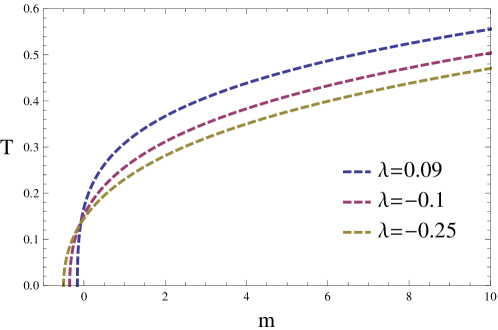
Figure 1: Hawking temperature $T$ versus the mass parameter $m$ for $d=4$. We have set $L=1$. The three curves are for $\lambda=-0.25,-0.1,0.09$, respectively, and they intersect at the AdS vacuum solution when $m=0$.

Going back to the $r$ coordinate, the metric becomes

$$ds^{2}=\frac{\rho^{2}}{1-H^{2}r^{2}}\left(-\frac{f(\rho)}{\rho^{2}}(1-H^{2}r^{2})dt^{2}+\frac{dr^{2}}{1-H^{2}r^{2}}+r^{2}d\Omega_{d-2}^{2}\right)+\frac{d\rho^{2}}{f(\rho)}~{},$$ (17)

whose boundary metric is just (or conformal to) the dS metric in static patch equation (6). Holographically, this bulk geometry is dual to the thermal quantum field theorie on the static patch of $dS_{d}$ at the temperature given by Eq.  (14). Note that this temperature does not have to be the same as the dS temperature $T_{dS}$, and this will yield a conical singularity in the manifold unless $T=T_{dS}$. We do not have to worry about this singularity since we only have interest on the physics outside the horizon, see more discussions about this point in Ref. Fischler:2013fba .

II.4 A Vaidya-like solution

To study the process of the thermalization in the boundary quantum field field theory the bulk should be holographically modelled by the process of a black hole formation. Thus, we need a Vaidya-like version of the black hole solution of Eq. (17). Defining an inverse radius $z=L^{2}/\rho$, going to Eddington-Finkstein coordinates and introducing a time-dependent mass parameter, we obtain the Vaidya-like bulk metric Fischler:2013fba

$$ds^{2}=\frac{L^{2}}{z^{2}}\left(-f(z,v)dv^{2}-2dvdz+\frac{H^{2}L^{2}}{(1-H^{2}r^{2})^{2}}dr^{2}+\frac{H^{2}L^{2}}{1-H^{2}r^{2}}r^{2}d\Omega_{d-2}^{2}\right)~{},$$ (18)

where the metric function in the presence of the Gauss-Bonnet term is

$$f(z,v)=\frac{z^{2}}{L^{2}}\bigg{[}-1+\frac{L^{2}}{2\lambda z^{2}}\left(1-\sqrt{1+4\lambda\left(m(v)z^{d}-1\right)}\right)\bigg{]}~{}.$$

To obtain (18) the equation of motion (3) has to be modified by introducing an external source,

$$R_{\mu\nu}-\frac{1}{2}Rg_{\mu\nu}-\frac{d(d-1)}{2L^{2}}g_{\mu\nu}+\frac{L^{2}\lambda}{(d-2)(d-3)}H_{\mu\nu}=8\pi GT_{\mu\nu}^{ext}~{}.$$ (19)

Substituting the Vaiya-like metric (18) into the above equation, one can obtain the energy-momentum tensor of the required external source,

$$8\pi GT_{\mu\nu}^{ext}=\frac{d-1}{2}z^{d-1}\frac{dm}{dv}\delta_{\mu v}\delta_{\nu v}~{},$$ (20)

which implies that the infalling shell is made of null dust. The mass function $m(v)$ can take two different forms as follows Fischler:2013fba :

• $m(v)=\frac{M}{2}\left(1-\tanh\frac{v}{v_{0}}\right)$ with $m_{min}<M<0$

  This choice is equivalent to preparing the field system in a state with $T<T_{dS}$ and then letting it evolve to the Bunch-Davies vacuum.

• $m(v)=\frac{M}{2}\left(1+\tanh\frac{v}{v_{0}}\right)$ with $M>0$

  This corresponds to a case that we start from the Bunch-Davies vacuum and then evolve to a state with $T>T_{dS}$.

In this paper, we will focus on the second choice with the geometric picture that a null dust shell falls from the boundary into the bulk to form a black hole. At the field theory side, it corresponds to a sudden injection of energy into the system and then let it evolves to thermal equilibrium.

III Nonlocal observables

In this section, we use three nonlocal observables–equal-time two-point function, Wilson loop and entanglement entropy–to probe the thermalization process. According to the holographic principle, these three probes in the saddle approximation correspond to some geometric quantities in the dual bulk geometry with a metric given by (18). It is expected that these observables provide insights into the thermalization process in the strongly coupled quantum field theories the boundary. We will study the time evolution behavior of these three observables after a quantum quench, and examine the influence of the Gauss-Bonnet factor and the spacetime dimensions in the thermalization process. Relying on numerical calculations and without loss of generality following Balasubramanian:2010ce ; Balasubramanian:2011ur , we will consider a thin shell with a small $v_{0}$, i.e., $v_{0}=0.01$, and we will set $L=1$ and fix the mass parameter to $M=1$.

III.1 Two-point function

Defining $\tilde{r}\equiv Hr$ and choosing two antipode points on the sphere $\tilde{r}=\tilde{R}$ on the boundary at the boundary time $\tilde{t}$, we can calculate the equal-time correlation function of some operator with large conformal dimension, which depends on $\tilde{t}$. Holographically, in the saddle approximation this two-point function corresponds to the length of the geodesic in the bulk which is anchored at the two points on the boundary. The geodesic $\gamma$ can be parametrized by two functions, $z(\tilde{r})$ and $v(\tilde{r})$, with other coordinates fixed respecting the spherical symmetry. With the Vaidya-like metric (18), we can obtain the induced metric on the geodesic, which is

$$ds_{\gamma}^{2}=\frac{L^{2}}{z^{2}}\left(\frac{L^{2}}{(1-\tilde{r}^{2})^{2}}-f(z,v)v^{\prime 2}-2v^{\prime}z^{\prime}\right)d\tilde{r}^{2}~{}.$$ (21)

Then, the length functional of the geodesic is

$${\cal L} = 2L\int_{0}^{\tilde{R}}\frac{d\tilde{r}}{z}Q~{},$$ (22)

$$Q \equiv \sqrt{\frac{L^{2}}{(1-\tilde{r}^{2})^{2}}-f(z,v)v^{\prime 2}-2v^{\prime}z^{\prime}}~{}.$$

To minimize the length of the geodesic, we need to solve the two equations of motion for $z(\tilde{r})$ and $v(\tilde{r})$, respectively, which are derived varying the length functional (22),

$$2(\tilde{r}^{2}-1)^{4}zv^{\prime 2}z^{\prime\prime}+\Bigg{\{}\left[6L^{2}(\tilde{r}^{2}-1)^{2}v^{\prime}-6(\tilde{r}^{2}-1)^{4}fv^{\prime 3}+(\tilde{r}^{2}-1)^{4}zv^{\prime}\left(3v^{\prime 2}\frac{\partial f}{\partial z}-2v^{\prime\prime}\right)\right]z^{\prime}$$

$$+(\tilde{r}^{2}-1)\left[4L^{2}\tilde{r}v^{\prime}+2L^{2}(\tilde{r}^{2}-1)v^{\prime\prime}-L^{2}(\tilde{r}^{2}-1)v^{\prime 2}\frac{\partial f}{\partial z}+(\tilde{r}^{2}-1)^{3}v^{\prime 4}\left(\frac{\partial f}{\partial v}+f\frac{\partial f}{\partial z}\right)\right]z$$

$$-2(\tilde{r}^{2}-1)^{4}f^{2}v^{\prime 4}-4(\tilde{r}^{2}-1)^{4}v^{\prime 2}z^{\prime 2}+4L^{2}(\tilde{r}^{2}-1)^{2}fv^{\prime 2}-2L^{4}\Bigg{\}}=0~{},$$ (23)

$$2(\tilde{r}^{2}-1)(L^{2}f+(\tilde{r}^{2}-1)^{2}z^{\prime 2})zv^{\prime\prime}+\Bigg{\{}(\tilde{r}^{2}-1)^{3}z^{\prime}\left[2f^{2}-z\frac{\partial f}{\partial v}-zf\frac{\partial f}{\partial z}\right]v^{\prime 3}$$

$$+\left[6(\tilde{r}^{2}-1)^{3}fz^{\prime 2}+L^{2}(\tilde{r}^{2}-1)z\frac{\partial f}{\partial v}-3(\tilde{r}^{2}-1)^{3}zz^{\prime 2}\frac{\partial f}{\partial z}\right]v^{\prime 2}$$

$$+\left[4L^{2}\tilde{r}fz-2L^{2}(\tilde{r}^{2}-1)fz^{\prime}+4(\tilde{r}^{2}-1)^{3}z^{\prime 3}-2(\tilde{r}^{2}-1)zz^{\prime}\left((\tilde{r}^{2}-1)^{2}z^{\prime\prime}-L^{2}\frac{\partial f}{\partial z}\right)\right]v^{\prime}$$

$$+2L^{2}\left[z(2\tilde{r}z^{\prime}+(r^{2}-1)z^{\prime\prime})-(\tilde{r}^{2}-1)z^{\prime 2}\right]\Bigg{\}}=0~{}.$$ (24)

Here prime denotes the derivative with respect to $\tilde{r}$, i.e., ${}^{\prime}\equiv\frac{d}{d\tilde{r}}$. To solve these equations, we need to consider the symmetry of the geodesic and impose the following boundary conditions

$$z(\epsilon)=z_{\ast}+{\cal O}(\epsilon^{2})~{},\quad z^{\prime}(\epsilon)=0+{\cal O}(\epsilon^{2})~{},$$ (25)

$$v(\epsilon)=v_{\ast}+{\cal O}(\epsilon^{2})~{},\quad v^{\prime}(\epsilon)=0+{\cal O}(\epsilon^{2})~{},$$

where $\epsilon$ is a small quantity, with order of $10^{-3}$ typically. To avoid the numerical problem at $\tilde{r}=0$ (note that $\tilde{r}=0$ is a singular point of Eq. (23) as $v^{\prime}(0)=0$ respecting the symmetry), we impose the boundary conditions at the neighborhood of the midpoint $\tilde{r}=0$, rather than exactly at the midpoint. The ${\cal O}(\epsilon^{2})$ terms above are the correction terms, and can be obtained by solving the two equations of motion around $\tilde{r}=0$ order by order. Here, we only calculate the equations to the order $\epsilon^{2}$. The two free parameters $z_{\ast}$ and $v_{\ast}$ are determined by the constraint equations

$$z(\tilde{R})=z_{0}~{},\quad v(\tilde{R})=\tilde{t}~{},$$ (26)

where $z_{0}$ is a UV cutoff and $\tilde{t}$ is the boundary time.

Using numerical methods, we can calculate the geodesic length ${\cal L}$ at any given time, which is cutoff dependent and divergent as $z_{0}\rightarrow 0$. To remove its dependence on the cutoff, one can define a relative geodesics length $\delta\bar{\cal L}\equiv\frac{{\cal L}-{\cal L}_{thermal}}{R_{rs}}$, with ${\cal L}_{thermal}$ being the length of the late time and $R_{rs}=L\ln\left(\frac{1+\tilde{R}}{1-\tilde{R}}\right)$ is the proper radial separation between the two points on the boundary. $\delta\bar{\cal L}$ is a function of the boundary time $\tilde{t}$ and $\tilde{R}$ is the boundary separation.

In Fig. 2, we plot the time evolution of $\delta\bar{\cal L}$ in five dimensions ($d=4$) for two boundary scales $\tilde{R}=0.3$ and $\tilde{R}=0.9$. We take the Gauss-Bonnet factor in a range bigger than the constraint (2) by choosing $\lambda=-0.25,-\frac{7}{36}(\text{lower bound}),-0.1,0,0.03,0.09(\text{upper bound}),0.2$, respectively. In Fig. 2 we can see the whole thermalization process. At very early time the evolution encounters a delay, especially for large $\tilde{R}$, then it follows a pre-local-equilibration stage during which the growth is quadratic in time; later, it appears in a post-local-equilibration stage of linear growth, and finally there emerges a period of memory loss prior to equilibration, after which the curves flatten out and the two-point functions reach their thermal equilibrium values.

For large $\tilde{R}$, it takes more time for the two-point function to reach thermal equilibrium value. This can be understood by the fact that the collapsing shell from the boundary passes the geodesic with larger length slower than the one with smaller length. These phenomena, disclosed in Fig. 2, are consistent with that observed in the flat boundary case Liu:2013iza ; Liu:2013qca ; Balasubramanian:2010ce ; Balasubramanian:2011ur and also in the Einstein dS boundary case Fischler:2013fba . They are universal and do not change in case that the high curvature corrections are considered in the gravity, even when the Gauss-Bonnet coupling constant $\lambda$ takes values beyond the constraint appearing in Eq.  (2).

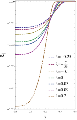
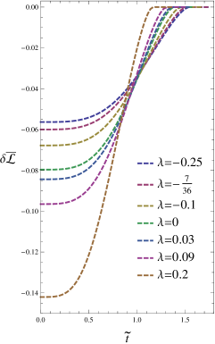
Figure 2: Time evolution of $\delta\bar{\cal L}$ in five dimensions ($d=4$) for the two boundary scale $\tilde{R}=0.3,0.9$, respectively. In each graph, on the left, from top to bottom, seven curves take Gauss-Bonnet coupling constant $\lambda=-0.25,-\frac{7}{36}(\text{lower bound}),-0.1,0,0.03,0.09(\text{upper bound}),0.2$, respectively.

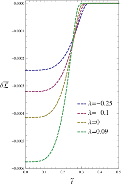
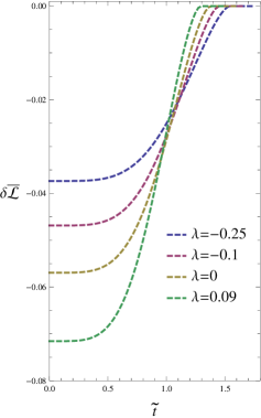
Figure 3: Time evolution of $\delta\bar{\cal L}$ in six dimensions ($d=5$) with the boundary scale $\tilde{R}=0.3,0.9$, respectively. In each graph, on the left, from top to bottom, four curves take Gauss-Bonnet coupling constant $\lambda=-0.25,-0.1,0,0.09$, respectively.

Although the Gauss-Bonnet factor does not alter qualitatively in the five successive processes of the thermalization, in Fig. 2 we do clearly see that it leaves imprints. The increase of the Gauss-Bonnet factor makes the initial absolute value of $\delta\bar{\cal L}$ to increase, which means that the dual field system is initially further away from the thermal equilibrium. However, the larger $\lambda$ makes the delay time shorter and the growth of $\delta\bar{\cal L}$ faster, so that the saturation time to reach thermal equilibrium decreases. The same phenomenon is also observed in higher dimensions, for example as shown in Fig. 3 with $d=5$. Comparing the results of the $d=4$ and $d=5$ cases, one can see that, for the fixed $\lambda$, the absolute initial value of $\delta\bar{\cal L}$ decreases as the spacetime dimension increases, while the delay time increases, which leaves the saturation time nearly unchanged. The dimensional influence can be seen more clearly in Fig. 4, where we exhibit the results of two fixed Gauss-Bonnet factors for different spacetime dimensions ($d=4$ and $d=5$).

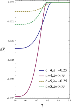
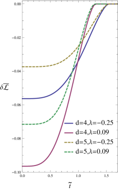
Figure 4: Time evolution of $\delta\bar{\cal L}$ in different dimensions ($d=4$ and $d=5$) with the boundary scale $\tilde{R}=0.3,0.9$, respectively.

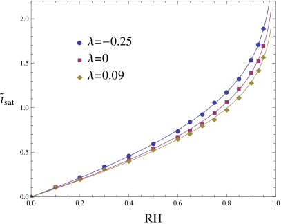
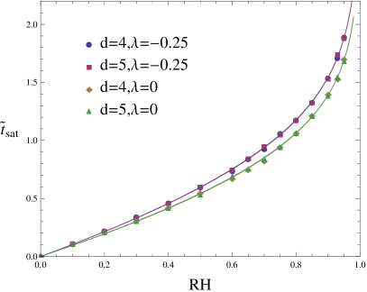
Figure 5: Saturation time $\tilde{t}_{sat}$ as a function of the boundary scale $\tilde{R}$. In the left plot we fix the spacetime dimension $d=4$. In the right panel, we compare the dimensional influence by choosing two values of the Gauss-Bonnet factor, $\lambda=-0.25$ and $\lambda=0$. Solid curves in both panels are produced by fitting the numerical points with function $a\tilde{R}+b\ln(1-\tilde{R})$.

We find that the saturation time $\tilde{t}$ is a key quantity to characterize the thermalization process: it decreases when the Gauss-Bonnet coupling constant increases, while it weakly depends on the spacetime dimensions.

From Figs. 2–4 we can further learn that the saturation time strongly depends on the boundary scale $\tilde{R}\equiv RH$. In Fig. 5, we plot the saturation time versus the boundary scale $\tilde{R}$. For small $\tilde{R}$, $\tilde{t}_{sat}$ increases linearly with $\tilde{R}$ and weakly depends on the Gauss-Bonnet constant, since the behavior should reduce to that of the flat boundary case there Balasubramanian:2010ce ; Balasubramanian:2011ur ; Zeng:2013mca ; Li:2013cja . However, as $\tilde{R}$ approaches the cosmological horizon, $\tilde{t}_{sat}$ blows up logarithmically and shows strong dependence on the Gauss-Bonnet factor. Moreover, from the right panel of Fig. 5 one can observe that there is not a clear influence on the saturation time measured by the two-point function which is due to the dimensionality of spacetime. As we will discuss in the next subsection the same behavior is observed also in the Wilson loop. To see an effect we have to study the entanglement entropy as the probe.

III.2 Wilson loop

In this subsection, we study the time evolution of the observable of the Wilson loop. On the boundary at time $\tilde{t}$, we choose an equator of a sphere with radius $\tilde{r}=\tilde{R}$, parametrized by the angular coordinate $\theta$, and calculate the expectation value of this Wilson loop, which depends on $\tilde{t}$. In the bulk, it corresponds to the area of a two-dimensional extremal surface $\Sigma$ anchored at the circle on the boundary. Considering the symmetry, the extremal surface $\Sigma$ can be parametrized by two functions, $z(\tilde{r})$ and $v(\tilde{r})$, and the induced metric on $\Sigma$ is

$$ds_{\Sigma}^{2}=\frac{L^{2}}{z^{2}}\left(\frac{L^{2}}{(1-\tilde{r}^{2})^{2}}-f(z,v)v^{\prime 2}-2v^{\prime}z^{\prime}\right)d\tilde{r}^{2}+\frac{L^{4}}{z^{2}}\frac{\tilde{r}^{2}}{1-\tilde{r}^{2}}d\theta^{2}~{}.$$ (27)

The area functional is given by

$${\cal A} = 2\pi L^{3}\int_{0}^{\tilde{R}}\frac{d\tilde{r}}{z^{2}}QP~{}.$$ (28)

$$Q \equiv \sqrt{\frac{L^{2}}{(1-\tilde{r}^{2})^{2}}-f(z,v)v^{\prime 2}-2v^{\prime}z^{\prime}}~{},\qquad P\equiv\frac{\tilde{r}}{\sqrt{1-\tilde{r}^{2}}}~{}.$$

To deduce the extreme value of this area functional, we need to solve the two equations of motion, which can be derived by varying the area functional

$$2\tilde{r}(\tilde{r}^{2}-1)^{4}zv^{\prime 2}z^{\prime\prime}+\Bigg{\{}-4\tilde{r}\left(L^{2}-(\tilde{r}^{2}-1)^{2}fv^{\prime 2}\right)^{2}-8\tilde{r}(\tilde{r}^{2}-1)^{4}v^{\prime 2}z^{\prime 2}$$

$$+\left[12\tilde{r}(\tilde{r}^{2}-1)^{2}v^{\prime}(L^{2}-(\tilde{r}^{2}-1)^{2}fv^{\prime 2})+(\tilde{r}^{2}-1)^{3}zv^{\prime}\left(4v^{\prime}-2\tilde{r}(\tilde{r}^{2}-1)v^{\prime\prime}+3\tilde{r}(\tilde{r}^{2}-1)v^{\prime 2}\frac{\partial f}{\partial z}\right)\right]z^{\prime}$$

$$+(\tilde{r}^{2}-1)\bigg{[}2L^{2}(2\tilde{r}^{2}-1)v^{\prime}+2(\tilde{r}^{2}-1)^{2}fv^{\prime 3}+2L^{2}\tilde{r}(\tilde{r}^{2}-1)v^{\prime\prime}-L^{2}\tilde{r}(\tilde{r}^{2}-1)v^{\prime 2}\frac{\partial f}{\partial z}$$

$$+\tilde{r}(\tilde{r}^{2}-1)^{3}v^{\prime 4}\left(\frac{\partial f}{\partial v}+f\frac{\partial f}{\partial z}\right)\bigg{]}z\Bigg{\}}=0~{},$$ (29)

$$2\tilde{r}(\tilde{r}^{2}-1)z\left(L^{2}f+(\tilde{r}^{2}-1)^{2}z^{\prime 2}\right)v^{\prime\prime}+\Bigg{\{}2L^{2}\left[z\left((2\tilde{r}^{2}-1)z^{\prime}+\tilde{r}(\tilde{r}^{2}-1)z^{\prime\prime}\right)-2\tilde{r}(\tilde{r}^{2}-1)z^{\prime 2}\right]$$

$$+(\tilde{r}^{2}-1)^{2}\left[2f^{2}\left(z+2\tilde{r}(\tilde{r}^{2}-1)z^{\prime}\right)-\tilde{r}(\tilde{r}^{2}-1)zz^{\prime}\left(\frac{\partial f}{\partial v}+f\frac{\partial f}{\partial z}\right)\right]v^{\prime 3}$$

$$+(\tilde{r}^{2}-1)\left[6(\tilde{r}^{2}-1)fz^{\prime}\left(z+2\tilde{r}(\tilde{r}^{2}-1)z^{\prime}\right)+\tilde{r}z\left(L^{2}\frac{\partial f}{\partial v}-3(\tilde{r}^{2}-1)^{2}z^{\prime 2}\frac{\partial f}{\partial z}\right)\right]v^{\prime 2}$$

$$+\bigg{[}2L^{2}(2r^{2}-1)fz-4L^{2}r(r^{2}-1)fz^{\prime}+4(r^{2}-1)^{2}zz^{\prime 2}+8r(r^{2}-1)^{3}z^{\prime 3}$$

$$-2\tilde{r}(\tilde{r}^{2}-1)zz^{\prime}\left((\tilde{r}^{2}-1)^{2}z^{\prime\prime}-L^{2}\frac{\partial f}{\partial z}\right)\bigg{]}v^{\prime}\Bigg{\}}=0~{}.$$ (30)

Again, to avoid the numerical problem at the midpoint $\tilde{r}=0$, we impose the boundary condition (25) at the neighborhood of the midpoint.

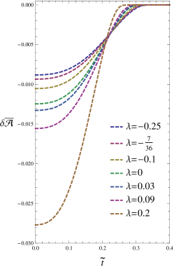
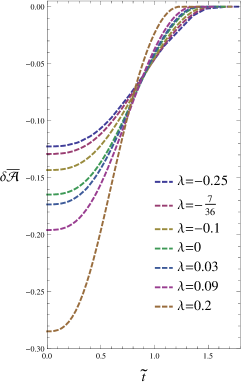
Figure 6: Time evolution of $\delta\bar{\cal A}$ in five dimensions ($d=4$) with the boundary scale $\tilde{R}=0.3,0.9$, respectively. In each graph, on the left, from top to bottom, seven curves take Gauss-Bonnet coupling constant $\lambda=-0.25,-\frac{7}{36}(\text{lower bound}),-0.1,0,0.03,0.09(\text{upper bound}),0.2$, respectively.

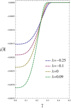
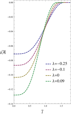
Figure 7: Time evolution of $\delta\bar{\cal A}$ in six dimensions ($d=5$) with the boundary scale $\tilde{R}=0.3,0.9$, respectively. In each graph, on the left, from top to bottom, four curves take Gauss-Bonnet coupling constant $\lambda=-0.25,-0.1,0,0.09$, respectively.

Now we study the time evolution of the related area $\delta\bar{\cal A}\equiv\frac{{\cal A}-{\cal A}_{thermal}}{A_{bny}}$, where $A_{bny}=2\pi L^{2}\left(\frac{1}{\sqrt{1-\tilde{R}^{2}}}-1\right)$ is the area of the disk bounded by the loop on the boundary. We list the results in Figs. 6-9, which present similar influences of the Gauss-Bonnet coupling and the spacetime dimensions to those observed in the two-point function. Fig. 9 shows the saturation time $\tilde{t}_{sat}$, which shows the same behavior as in Fig. 5 of the two point function. For big boundary scale, the saturation time deduced from the Wilson loop exhibits the consistent behaviors with those from the two-point function, it decreases as the Gauss-Bonnet factor increases, but it depends very mildly on the spacetime dimensions.

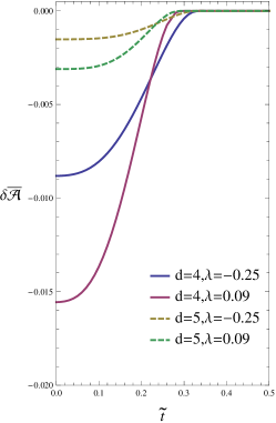
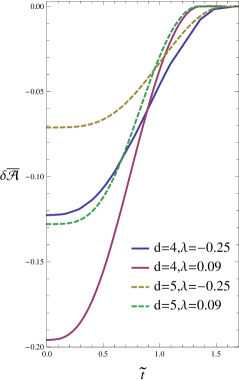
Figure 8: Time evolution of $\delta\bar{\cal A}$ in different dimensions ($d=4$ and $d=5$) and with the boundary scale $\tilde{R}=0.3,0.9$, respectively.

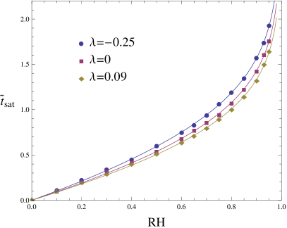
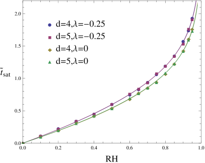
Figure 9: Saturation time $\tilde{t}_{sat}$ as a function of the boundary scale $\tilde{R}$. The left plot has fixed spacetime dimension $d=4$. In the right panel the comparison of the spacetime dimensional influence for chosen Gauss-Bonnet factors has been given. Solid curves in both panels are produced by fitting the numerical points with function $a\tilde{R}+b\ln(1-\tilde{R})$.

III.3 Entanglement Entropy

III.3.1 Holographic Entanglement Entropy Formula with Gauss-Bonnet Correction

Now we move on to study the observable of the entanglement entropy to see how it can be used to measure the thermalization process. Suppose the system of the quantum field theory in the boundary dS space is divided into two parts $A$ and $A^{c}$, where $A^{c}$ is the complement of $A$. Then we can define entanglement entropy of the region $A$ as the Von Neuman entropy,

$$S_{A}=-{\mathrm{t}r_{A}}\rho_{A}\log\rho_{A}~{},$$ (31)

where $\rho_{A}$ is the reduced density matrix of $A$.

Generally, it is hard to calculate the entanglement entropy from quantum field theory directly. However, AdS/CFT provides a powerful tool to deal with this problem. A holographic entanglement entropy has been proposed to relate this entropy to some geometric quantity of the dual bulk geometry. In Einstein gravity, the holographic entanglement entropy formula is Ryu:2006bv ; Hubeny:2007xt

$$S_{A}=\frac{1}{4G_{N}^{(d+1)}}{\rm ext}[{\rm Area}(\gamma_{A})]~{},$$ (32)

where $\gamma_{A}$ is the extremal codimensional two surface in the bulk with the boundary $\partial\gamma_{A}=\partial A$.

For higher derivative gravity theory, such as the Gauss-Bonnet gravity we are considering, the holographic entanglement formula is modified to be deBoer:2011wk ; Hung:2011xb ; Myers:2013lva ; Dong:2013qoa ; Camps:2013zua

$$S_{\rm HEE}=\frac{1}{4G_{N}^{(d+1)}}\int_{\gamma_{A}}\sqrt{\gamma}\left[1+\frac{2L^{2}\lambda}{(d-2)(d-3)}{\cal R}_{\gamma_{A}}\right]+\frac{1}{G_{N}^{(d+1)}}\frac{L^{2}\lambda}{(d-2)(d-3)}\int_{\partial\gamma_{A}}\sqrt{h}\ {\cal K}~{}.$$ (33)

The integration is done on the extremal surface ${\gamma_{A}}$. ${\cal R}_{\gamma_{A}}$ is the intrinsic curvature scalar of $\gamma_{A}$, which is the contribution due to the Gauss-Bonnet term. The last term is added to make the variation problem well defined. $h$ is the determinant of the induced metric on $\partial\gamma_{A}$, and ${\cal K}$ is the trace of the extrinsic curvature of $\partial\gamma_{A}$.

For a warped geometry with the following metric

$$ds^{2}=ds_{X}^{2}+\sum_{i}e^{2F_{i}(X)}ds_{Y_{i}}^{2}~{},$$ (34)

we have the formulae Hung:2011xb

$$R=R^{X}+\sum_{i}\left[e^{-2F_{i}}R^{Y_{i}}-2d_{i}(\nabla^{2}F_{i})-d_{i}(\partial F_{i})^{2}\right]-\sum_{i,j}d_{i}d_{j}(\partial F_{i}\cdot\partial F_{j})~{},$$ (35)

where $X$ and $Y_{i}$ are subspaces of the manifold and $d_{i}$ is the dimension of $Y_{i}$. $F_{i}(X)$ is the warped factor which depends only on the coordinates of $X$. All derivatives are evaluated in the $X$ space and $\nabla$ denotes the covariant derivative compatible with metric on $X$. In this subsection, the number of dimension of $X$ space is only $1$ and then $R^{X}=0$, and the space $Y$ is a $(d-2)$-dimensional sphere. Calculating the holographic entanglement entropy by using the formula (35), we have

$$S_{\rm HEE}=\frac{1}{4G_{N}^{(d+1)}}\Omega_{d-2}\int dX\ \sqrt{h_{XX}}e^{(d-2)F}\left[1+2L^{2}\lambda\left(e^{-2F}+h^{XX}F^{\prime 2}\right)\right]~{}.$$ (36)

III.3.2 Time Evolution of Holographic Entanglement Entropy

On the boundary at time $\tilde{t}$, we choose the entangled region $A$ to be a $(d-1)$-dimensional sphere with $\tilde{r}=0$ as the original point. Considering the symmetry, the extremal codimensional two surface $\gamma_{A}$ in the bulk can be parametrized by functions $z(\tilde{r})$ and $v(\tilde{r})$. The induced metric on $\gamma_{A}$ is

$$ds_{\Sigma}^{2}=\frac{L^{2}}{z^{2}}\left(\frac{L^{2}}{(1-\tilde{r}^{2})^{2}}-f(z,v)v^{\prime 2}-2v^{\prime}z^{\prime}\right)d\tilde{r}^{2}+\frac{L^{4}}{z^{2}}\frac{\tilde{r}^{2}}{1-\tilde{r}^{2}}d\Omega_{d-2}^{2}~{},$$ (37)

which takes a form as in (34). With the formula of Eq. (36), the holographic entanglement entropy functional becomes

$${\cal S} = \frac{L^{2d-3}}{4G_{N}^{(d+1)}}\Omega_{d-2}\int_{0}^{\tilde{R}}\frac{d\tilde{r}}{z^{d-1}}QP^{d-2}\left[1+\frac{2\lambda z^{2}}{L^{2}}\left(P^{-2}+L^{2}Q^{-2}\left(\frac{P^{\prime}}{P}-\frac{z^{\prime}}{z}\right)^{2}\right)\right]~{}.$$ (38)

$$Q \equiv \sqrt{\frac{L^{2}}{(1-\tilde{r}^{2})^{2}}-f(z,v)v^{\prime 2}-2v^{\prime}z^{\prime}}~{},\qquad P\equiv\frac{\tilde{r}}{\sqrt{1-\tilde{r}^{2}}}~{}.$$

As done in the above two subsections, we need to solve the two equations of motion to get the extreme value of the holographic entanglement entropy functional. The two equations of motion are very complicated and we do not show them explicitly here. We adopt the same boundary conditions of (25) in doing the computation.

For convenience, we define the relative holographic entanglement entropy $\delta\bar{{\cal S}}\equiv\frac{{\cal S}-{\cal S}_{thermal}}{V_{b}}$, where $V_{b}=L^{d-1}\Omega_{d-2}\int_{0}^{\tilde{R}}\frac{\tilde{r}^{d-2}}{(1-\tilde{r}^{2})^{d/2}}d\tilde{r}=L^{d-1}\Omega_{d-2}\frac{\tilde{R}^{d-1}}{d-1}~{}_{2}F_{1}\left(\frac{d-1}{2},\frac{d}{2},\frac{d+1}{2},\tilde{R}^{2}\right)$ is the volume of the entangled region $A$ on the boundary. In Fig. 10, we plot the time evolution of $\delta\bar{{\cal S}}$ with various Gauss-Bonnet coupling constant $\lambda$ for chosen size $\tilde{R}$ of the entangled sphere. The disclosed saturation time decreases as $\lambda$ increases, which is consistent with the results of the previous two observables. Comparing with the previous two observables, we observe that the delay time in the onset of thermalization becomes shorter as shown in the entanglement entropy. This can be understood, since the entanglement entropy is related more to the degrees of freedom of the system so that it is more sensitive to the thermalization process.

Looking at the initial absolute value of $\delta\bar{{\cal S}}$, we surprisingly find that with the increase of $\lambda$, it becomes smaller, instead of becoming bigger. This means that the initial state of the field system due to the higher curvature correction terms in the gravity is closer to the thermal equilibrium state, which is completely different from the results of the previous two observables. The relation of the thermalization process to the Gauss-Bonnet factor holds as well when we fix the spacetime dimension to be $d=5$ as shown in Fig. 11.

In Fig. 12, we show the spacetime dimensional influence on the thermalization process reflected by the entanglement entropy. It is clear that with the increase of the spacetime dimension, the initial absolute value of $\delta\bar{{\cal S}}$ increases, while the saturation time decreases. This is displayed more clearly in Fig. 13, where the saturation time $\tilde{t}_{sat}$ versus the size of the entangled sphere is plotted. Comparing with the other two observables, the entanglement entropy reflects more clearly the dependence of the saturation time on the spacetime dimensions, especially for large $\tilde{R}$. This is expected, since the two-point function and the Wilson loop are only related to the degrees of freedom on the two points and the loop respectively, while the entanglement entropy is related to the degrees of freedom in the volume of the bounded region $A$ which depends strongly on the spacetime dimensions. This point can also be seen by comparing definitions of these three observables in Eqs. (22),(28) and (38). From Fig. 13, it is clearly shown that the saturation time decreases as $d$ increases. Physically, we can understand this phenomenon, since quanta in higher dimensions have more degrees of freedom to collide and interact with neighboring quanta, and thus thermalize faster.

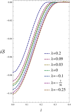
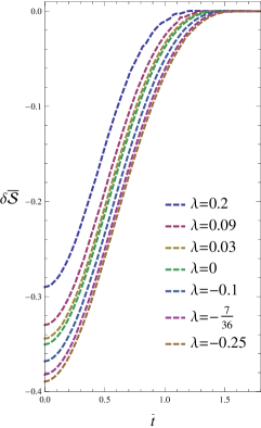
Figure 10: Time evolution of $\delta\bar{{\cal S}}$ in $d=4$ case. From left to right, the rescaled radius of the entangled sphere are $\tilde{R}=0.3,0.9$, respectively. In each figure, the Gauss-Bonnet coupling constant $\lambda$, from top to bottom, are taken to be $0.2,0.09,0.03,0,-0.1,-\frac{7}{36},-0.25$.

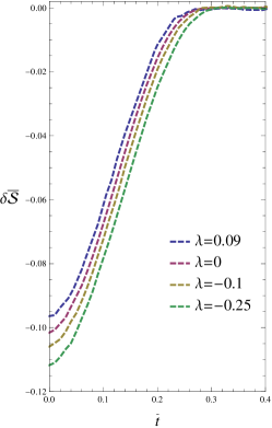
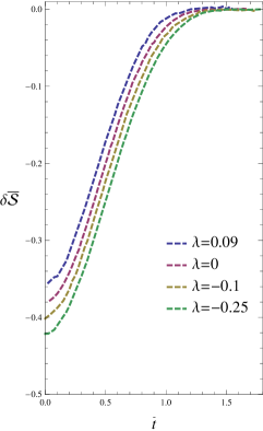
Figure 11: Time evolution of $\delta\bar{{\cal S}}$ in $d=5$ case, the rescaled radius of the entangled sphere $\tilde{R}=0.3,0.9$, respectively. In each figure, the Gauss-Bonnet coupling constant $\lambda$, from top to bottom, are taken to be $0.09,0,-0.1,-0.25$.

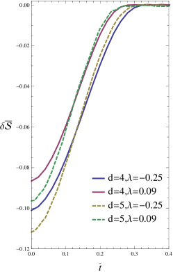
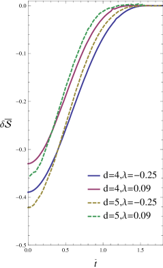
Figure 12: Time evolution of $\delta\bar{{\cal S}}$ in $d=4$ and $d=5$ cases. From left to right, The rescaled radius of the entangled sphere are $\tilde{R}=0.3,0.9$ respectively.

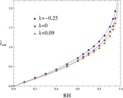
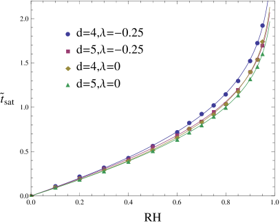
Figure 13: Saturation time $\tilde{t}_{sat}$ as a function of the boundary scale $\tilde{R}$. The left panel is for $d=4$. The right panel is the comparison of the dimensional influence by fixing the Gauss-Bonnet factor. Solid curves in both panels are produced by fitting the numerical points with function $a\tilde{R}+b\ln(1-\tilde{R})$. There is a large overlap between the curve with $(d=4,\lambda=0)$ and the one with $(d=5,\lambda=-0.25)$.

IV Conclusions and discussion

In this work we have discussed the holographic thermalization process by relating gravity theory with higher curvature corrections to the dual strongly coupled quantum field theory living on the dS boundary. We found that the whole thermalization process follows the general pattern observed in Fischler:2013fba . At very early time the evolution of the thermalization encounters a delay, then it enters the pre-local-equilibration stage during which the growth is quadratic in time. Afterwards we have the post-local-equilibration stage of linear growth, and finally there emerges a period of memory loss, after which the curves flatten out and the observables reach their thermal values.

Our findings follow some universal properties, as observed in the Einstein case with flat Liu:2013iza ; Liu:2013qca ; Balasubramanian:2010ce ; Balasubramanian:2011ur or with curved Fischler:2013fba boundary, but also they show some district features due to the presence of higher curvature correction term in the bulk. As we discussed in the Introduction, a delay in the onset of thermalization was found. In our case for large boundary scales $\tilde{R}$ we also observed a delay on the onset of thermalization for the two probes, the two-point function and the Wilson loop, while the onset of thermalization becomes much shorter for the third probe, the entanglement entropy.

In Einstein gravity the saturation time, i.e the time needed the system to reach thermal equilibrium is very fast. In our study for larger boundary scales $\tilde{R}$ it takes more time for the system to reach thermal equilibrium and this result holds for all the three probes. However, as the strength of the Gauss-Bonnet coupling $\lambda$ is increased, the saturation time of the thermalization process becomes shorter as the entanglement entropy shows. This is interesting because it relates directly the straight of gravity effects to the time that the system on the boundary needs to reach thermal equilibrium.

In Einstein gravity the thermalization process seems to be independent of dimensionality. In the presence of the higher curvature correction term in the bulk the two probes the two-point function and the Wilson loop show the same behavior. However, the entanglement entropy shows clearly a spacial dependence of the thermalization process. This can be attributed to the fact that the holographic entanglement entropy contains more bulk information and is more sensitive to the spacetime dimensions. We have found that the thermalization process as probed by the entanglement entropy is faster in the spacetime with higher dimensions. This can be understood since quanta in higher dimensions have more degrees of freedom to collide and interact with neighboring quanta, which makes the thermalization quicker.

It is interesting to investigate further the effect of a nontrivial gravity bulk on the thermalization process. A way to study this effect is to consider a scalar field collapsing in an AdS space. Following this approach it was found danielsson ; janik1 ; chesler ; garfinkle ; Garfinkle:2011tc that for a collapsing scalar field minimally coupled to gravity the thermalization process proceeds very rapidly. One can introduce a nonminimal coupling like a coupling of a scalar field to Einstein tensor and investigate the thermalization process on the boundary. Work in this direction is in progress.

References

- (1) J. M. Maldacena, The Large N limit of superconformal field theories and supergravity, Int. J. Theor. Phys. 38, 1113 (1999) [Adv. Theor. Math. Phys. 2, 231 (1998)] [hep-th/9711200].
- (2) S. S. Gubser, I. R. Klebanov and A. M. Polyakov, Gauge theory correlators from noncritical string theory, Phys. Lett. B 428, 105 (1998) [hep-th/9802109].
- (3) E. Witten, Anti-de Sitter space and holography, Adv. Theor. Math. Phys. 2, 253 (1998) [hep-th/9802150].
- (4) G. T. Horowitz, Introduction to Holographic Superconductors, Lect. Notes Phys. 828, 313 (2011) [arXiv:1002.1722 [hep-th]].
- (5) S. A. Hartnoll, Lectures on holographic methods for condensed matter physics, Class. Quant. Grav. 26, 224002 (2009) [arXiv:0903.3246 [hep-th]].
- (6) F. Gelis, The Early Stages of a High Energy Heavy Ion Collision, J. Phys. Conf. Ser. 381, 012021 (2012) [arXiv:1110.1544 [hep-ph]].
- (7) E. Iancu, QCD in heavy ion collisions, arXiv:1205.0579 [hep-ph].
- (8) B. Muller and A. Schafer, Entropy Creation in Relativistic Heavy Ion Collisions, Int. J. Mod. Phys. E 20, 2235 (2011) [arXiv:1110.2378 [hep-ph]].
- (9) J. Casalderrey-Solana, H. Liu, D. Mateos, K. Rajagopal and U. A. Wiedemann, Gauge/String Duality, Hot QCD and Heavy Ion Collisions, arXiv:1101.0618 [hep-th].
- (10) E. Shuryak, Why does the quark gluon plasma at RHIC behave as a nearly ideal fluid?, Prog. Part. Nucl. Phys. 53, 273 (2004) [hep-th/0312227].
- (11) G. Policastro, D.T. Son, A.O. Starinets, Shear viscosity of strongly coupled supersymmetric Yang-Mills plasma, Phys. Rev. Lett. 87, 081601 (2001) [hep-th/0104066].
- (12) D. T. Son, A. O. Starinets, Viscosity, Black Holes, and Quantum Field Theory, Ann. Rev. Nucl. Part. Sci. 57, 95 (2007) [arxiv:0704.0240[hep-th]].
- (13) G. Policastro, D.T. Son, A.O. Starinets, From AdS/CFT correspondence to hydrodynamics, JHEP 09, 043 (2002) [hep-th/0205052].
- (14) S. Bhattacharyya, V.E. Hubeny, S. Minwalla and M. Rangamani, Nonlinear fluid dynamics from gravity, J. High Energy Phys. 0802, 045 (2008) [arXiv:0712.2456 [hep-th]].
- (15) P. K. Kovtun and A. O. Starinets, Quasinormal modes and holography, Phys. Rev. D 72, 086009 (2005) [hep-th/0506184].
- (16) M. Brigante, H. Liu, R. C. Myers, S. Shenker and S. Yaida, Viscosity Bound Violation in Higher Derivative Gravity, Phys. Rev. D 77, 126006 (2008) [arXiv:0712.0805 [hep-th]].
- (17) M. Brigante, H. Liu, R. C. Myers, S. Shenker and S. Yaida, The Viscosity Bound and Causality Violation, Phys. Rev. Lett. 100, 191601 (2008) [arXiv:0802.3318 [hep-th]].
- (18) Y. Kats and P. Petrov, Effect of curvature squared corrections in AdS on the viscosity of the dual gauge theory, JHEP 0901, 044 (2009) [arXiv:0712.0743 [hep-th]].
- (19) G. Koutsoumbas, E. Papantonopoulos and G. Siopsis, Shear Viscosity and Chern-Simons Diffusion Rate from Hyperbolic Horizons, Phys. Lett. B 677, 74 (2009) [arXiv:0809.3388 [hep-th]].
- (20) R. Baier, A. H. Mueller, D. Schiff and D. T. Son, Bottom up’ thermalization in heavy ion collisions, Phys. Lett. B 502, 51 (2001) [hep-ph/0009237].
- (21) A. H. Mueller, A. I. Shoshi and S. M. H. Wong, A Possible modified ’bottom-up’ thermalization in heavy ion collisions, Phys. Lett. B 632, 257 (2006) [hep-ph/0505164].
- (22) U.H. Danielsson, E. Keski-Vakkuri and M. Kruczenski, Black hole formation in AdS and thermalization on the boundary, JHEP 02, 039 (2000) [hep-th/9912209].
- (23) R.A. Janik and R.B. Peschanski, Gauge/gravity duality and thermalization of a boost-invariant perfect fluid, Phys. Rev. D 74, 046007 (2006) [hep-th/0606149].
- (24) P.M. Chesler and L.G. Yaffe, Boost invariant flow, black hole formation and far-from-equilibrium dynamics in N = 4 supersymmetric Yang-Mills theory, Phys. Rev. D 82, 026006 (2010) [arXiv:0906.4426[hep-th]].
- (25) D. Garfinkle, L.A.P. Zayas, Rapid Thermalization in Field Theory from Gravitational Collapse, Phys. Rev. D 84, 066006 (2011) [arXiv:1106.2339[hep-th]].
- (26) D. Garfinkle, L. A. Pando Zayas and D. Reichmann, On Field Theory Thermalization from Gravitational Collapse, JHEP 1202, 119 (2012) [arXiv:1110.5823 [hep-th]].
- (27) S. Bhattacharyya and S. Minwalla, Weak field black hole formation in asymptotically AdS spacetimes, JHEP 09, 034 (2009) [arXiv:0904.0464 [hep-th]].
- (28) S. Lin and E. Shuryak, Toward the AdS/CFT gravity dual for high energy collisions. 3. Gravitationally collapsing shell and quasiequilibrium, Phys. Rev. D 78, 125018 (2008) [arXiv:0808.0910 [hep-th]].
- (29) V. Balasubramanian, A. Bernamonti, J. de Boer, N. Copland, B. Craps, E. Keski-Vakkuri, B. Muller and A. Schafer et al., Thermalization of Strongly Coupled Field Theories, Phys. Rev. Lett. 106, 191601 (2011) [arXiv:1012.4753 [hep-th]].
- (30) V. Balasubramanian, A. Bernamonti, J. de Boer, N. Copland, B. Craps, E. Keski-Vakkuri, B. Muller and A. Schafer et al., Holographic Thermalization, Phys. Rev. D 84, 026010 (2011) [arXiv:1103.2683 [hep-th]].
- (31) T. Hirayama, A Holographic dual of CFT with flavor on de Sitter space, JHEP 0606, 013 (2006) [hep-th/0602258].
- (32) K. Ghoroku, M. Ishihara and A. Nakamura, Gauge theory in de Sitter space-time from a holographic model, Phys. Rev. D 74, 124020 (2006) [hep-th/0609152].
- (33) D. Marolf, M. Rangamani and M. Van Raamsdonk, Holographic models of de Sitter QFTs, Class. Quant. Grav. 28, 105015 (2011) [arXiv:1007.3996 [hep-th]].
- (34) A. Buchel and D. A. Galante, Cascading gauge theory on and String Theory landscape, Nucl. Phys. B 883, 107 (2014) [arXiv:1310.1372 [hep-th]].
- (35) W. Fischler, S. Kundu and J. F. Pedraza, Entanglement and out-of-equilibrium dynamics in holographic models of de Sitter QFTs, JHEP 1407, 021 (2014) [arXiv:1311.5519 [hep-th]].
- (36) W. Fischler, P. H. Nguyen, J. F. Pedraza and W. Tangarife, Fluctuation and dissipation in de Sitter space, JHEP 1408, 028 (2014) [arXiv:1404.0347 [hep-th]].
- (37) H. Liu and S. J. Suh, Entanglement Tsunami: Universal Scaling in Holographic Thermalization, Phys. Rev. Lett. 112, 011601 (2014) [arXiv:1305.7244 [hep-th]].
- (38) H. Liu and S. J. Suh, Entanglement growth during thermalization in holographic systems, Phys. Rev. D 89, 066012 (2014) [arXiv:1311.1200 [hep-th]].
- (39) D. Galante and M. Schvellinger, Thermalization with a chemical potential from AdS spaces, JHEP 07, 096 (2012) [arXiv:1205.1548 [hep-th]].
- (40) E. Caceres and A. Kundu, Holographic Thermalization with Chemical Potential, JHEP 09, 055 (2012) [arXiv:1205.2354 [hep-th]].
- (41) G. Camilo, B. Cuadros-Melgar and E. Abdalla, Holographic thermalization with a chemical potential from Born-Infeld electrodynamics, arXiv:1412.3878 [hep-th].
- (42) X.-X. Zeng, W.-B. Liu, Holographic thermalization in Gauss-Bonnet gravity, Phys. Lett. B 726, 481 (2013) [arXiv:1305.4841 [hep-th]].
- (43) Y. Z. Li, S. F. Wu and G. H. Yang, Gauss-Bonnet correction to Holographic thermalization: two-point functions, circular Wilson loops and entanglement entropy, Phys. Rev. D 88, 086006 (2013) [arXiv:1309.3764 [hep-th]].
- (44) I. Aref’eva, A. Bagrov and A.S. Koshelev, Holographic thermalization from Kerr-AdS, JHEP 07, 170 (2013) [arXiv:1305.3267 [hep-th]].
- (45) X.-X. Zeng, X.-M. Liu, W.-B. Liu, Holographic thermalization in noncommutative geometry, [arXiv:1407.5262 [hep-th]].
- (46) M. Alishahiha, A. F. Astaneh and M. R. M. Mozaffar, Thermalization in backgrounds with hyperscaling violating factor, Phys. Rev. D 90, 046004 (2014) [arXiv:1401.2807 [hep-th]].
- (47) P. Fonda et al., Holographic thermalization with Lifshitz scaling and hyperscaling violation, JHEP 1408, 051 (2014) [arXiv:1401.6088 [hep-th]].
- (48) J. de Boer, M. Kulaxizi and A. Parnachev, Holographic Entanglement Entropy in Lovelock Gravities, JHEP 1107, 109 (2011) [arXiv:1101.5781 [hep-th]].
- (49) L. Y. Hung, R. C. Myers and M. Smolkin, On Holographic Entanglement Entropy and Higher Curvature Gravity, JHEP 1104, 025 (2011) [arXiv:1101.5813 [hep-th]].
- (50) R. C. Myers, R. Pourhasan and M. Smolkin, On Spacetime Entanglement, JHEP 1306, 013 (2013) [arXiv:1304.2030 [hep-th]].
- (51) X. Dong, Holographic Entanglement Entropy for General Higher Derivative Gravity, JHEP 1401, 044 (2014) [arXiv:1310.5713 [hep-th]].
- (52) J. Camps, Generalized entropy and higher derivative Gravity, JHEP 1403, 070 (2014) [arXiv:1310.6659 [hep-th]].
- (53) S. Ryu and T. Takayanagi, Holographic derivation of entanglement entropy from AdS/CFT, Phys. Rev. Lett. 96, 181602 (2006) [hep-th/0603001].
- (54) A. Buchel and R. C. Myers, Causality of Holographic Hydrodynamics, JHEP 0908, 016 (2009) [arXiv:0906.2922 [hep-th]].
- (55) X. O. Camanho and J. D. Edelstein, Causality constraints in AdS/CFT from conformal collider physics and Gauss-Bonnet gravity, JHEP 1004, 007 (2010) [arXiv:0911.3160 [hep-th]].
- (56) A. Buchel, J. Escobedo, R. C. Myers, M. F. Paulos, A. Sinha and M. Smolkin, Holographic GB gravity in arbitrary dimensions, JHEP 1003, 111 (2010) [arXiv:0911.4257 [hep-th]].
- (57) C. Fefferman and C. R. Graham, Conformal invariants, in lie Cartan et les Mathmatiques d’Aujourd’hui, (Astrisque, 1985), 95.
- (58) T. S. Bunch and P. C. W. Davies, Quantum Field Theory in de Sitter Space: Renormalization by Point Splitting, Proc. Roy. Soc. Lond. A 360, 117 (1978).
- (59) R. G. Cai, Gauss-Bonnet black holes in AdS spaces, Phys. Rev. D 65, 084014 (2002) [hep-th/0109133].
- (60) R. Emparan, AdS membranes wrapped on surfaces of arbitrary genus, Phys. Lett. B 432, 74 (1998) [hep-th/9804031].
- (61) D. Birmingham, Topological black holes in Anti-de Sitter space, Class. Quant. Grav. 16, 1197 (1999) [hep-th/9808032].
- (62) R. Emparan, AdS / CFT duals of topological black holes and the entropy of zero energy states, JHEP 9906, 036 (1999) [hep-th/9906040].
- (63) L. Vanzo, Black holes with unusual topology, Phys. Rev. D 56, 6475 (1997) [gr-qc/9705004].
- (64) X. Zeng and W. Liu, Holographic thermalization in Gauss-Bonnet gravity, Physics Letters B 726, 481 (2013) [arXiv:1305.4841 [hep-th]].
- (65) V. E. Hubeny, M. Rangamani and T. Takayanagi, A Covariant holographic entanglement entropy proposal, JHEP 0707, 062 (2007) [arXiv:0705.0016 [hep-th]].