Thawing quintessence from the inflationary epoch to today

Abstract

Using the latest observational data we obtain a lower bound on the initial value of the quintessence field in thawing quintessence models of dark energy. For potentials of the form $V(\phi)\sim\phi^{\pm 2}$ we find that the initial value $|\phi_{i}|>7\times 10^{18}{\rm\,Ge\kern-1.25ptV}$. We then relate $\phi_{i}$ to the duration of inflation by assuming that the initial value of the quintessence field is determined by quantum fluctuations of the quintessence field during inflation. From the lower bound on $\phi_{i}$ we obtain a lower bound on the number of e-foldings of inflation, namely, $N>2\times 10^{11}$. We obtain similar bounds for other power law potentials for which too we obtain $|\phi_{i}|>O(M_{P})$.

I Introduction

Cosmological observations Riess:1998cb ; Perlmutter:1998np ; Tonry:2003zg of the past one and a half decades indicate that the Universe is undergoing accelerated expansion. Although a non-zero cosmological constant can explain the current acceleration of the Universe, one still has to explain why it is so small and why only at recent times it has started to dominate the energy density of the Universe Zlatev:1998tr . These issues have motivated the exploration of alternative theories to explain the late time acceleration as due to a source of energy referred to as dark energy Copeland:2006wr ; Li:2011sd . A quintessence model is one amongst such theories where the dark energy arises from a scalar field $\phi$ rolling slowly down a potential.

The equation of state parameter $w$ can be defined as the ratio of the pressure to the energy density

$$w=p/\rho.$$ (1)

A cosmological constant is equivalent to $w=-1$ whereas a quintessence field generates a time dependent equation of state $w(t)>-1$. Caldwell and Linder Caldwell:2005tm showed that the quintessence models in which the scalar field rolls down its potential towards a minimum can be classified into two categories, namely $\it{freezing}$ and $\it{thawing}$ models, with quite different behavior. In thawing models at early times the field gets locked at a value away from the minimum of the potential due to large Hubble damping. At late times when Hubble damping diminishes, the field starts to roll down towards the minimum. These models have a value of $w$ which begins near $-1$ and gradually increases with time. In freezing models the field rolls towards its potential minimum initially and slows down at late times as it comes to dominate the Universe. These models have a value of $w$ which decreases with time. In both cases $w$ $\approx-1$ around the present epoch. Thawing models with a nearly flat potential provide a natural way to produce a value of $w$ that stays close to, but not exactly equal to $-1$. The field begins with $w\approx-1$ at high redshifts, and $w$ increases only slightly by low redshifts. These models depend on initial field values (in contrast with freezing models of quintessence which depend on the shape of the potential).

In the present work we evaluate the cosmological consequences of the evolving quintessence field in the context of thawing models by considering various observational datasets and obtain plausible initial values of the scalar field $\phi_{i}$ . A lower bound on the the allowed values of $\phi_{i}$ has been previously obtained in Ref. Gupta:2011ip . Our current numerical analysis provides stronger constraints on $\phi_{i}$. We further relate the initial value to quantum fluctuations of $\phi$ during inflation and thereby to the duration of inflation. The lower bound on $\phi_{i}$ then provides a lower bound on the number of e-foldings of inflation in our scenario where the initial value of the quintessence field is determined by quantum fluctuations of the field during inflation. Our work in this article is organised as follows. In section II we describe the thawing quintessence model in the standard minimal framework. In section III we provide a detailed description of the datasets used to obtain the observational constraints on the parameters of the model. In section IV we use the results obtained in our investigation to obtain a lower bound on the initial value of $\phi$. We then discuss the generation of the initial value by quantum fluctuations during inflation and use the lower bound on $\phi_{i}$ to obtain a lower bound on the number of e-foldings of inflation, $N$. We end with our conclusions in section V.

II The Thawing Quintessence Scenario

We will assume that the dark energy is provided by a minimally coupled scalar field $\phi$ with the equation of motion for the homogeneous component given by

$$\ddot{\phi}+3H\dot{\phi}+\frac{dV}{d\phi}=0\,,$$ (2)

where the Hubble parameter $H$ is given by

$$H=\left(\frac{\dot{a}}{a}\right)=\sqrt{\rho/3M^{2}_{P}}\,.$$ (3)

Here $a(t)$ is the scale factor, $\rho$ is the total density, and $M_{P}=(8\pi G)^{-1/2}=2.4\times 10^{18}{\rm\,Ge\kern-1.25ptV}$ is the reduced Planck mass. Eq. (2) indicates that while the field rolls downhill in the potential $V(\phi)$, its motion is damped by a term proportional to $H$. The pressure and density of the scalar field are given by

$$p=\frac{\dot{\phi}^{2}}{2}-V(\phi)$$ (4)

and

$$\rho=\frac{\dot{\phi}^{2}}{2}+V(\phi)$$ (5)

respectively, and the equation of state parameter $w$ is given by Eq. (1). At late times, the Universe is dominated by dark energy due to $\phi$, and non-relativistic matter. We assume a flat Universe so that $\Omega_{\phi}+\Omega_{m}+\Omega_{r}=1$. Then Eqs. (2) and (3) can be rewritten in terms of the variables $x$, $y$, and $\lambda$ defined by

$$x \equiv \phi^{\prime}/(M_{P}\sqrt{6})\,,$$ (6)

$$y \equiv \sqrt{V(\phi)/(3H^{2}M^{2}_{P})}\,,$$ (7)

$$\lambda \equiv -\frac{M_{P}}{V}\frac{dV}{d\phi}\,,$$ (8)

where the prime denotes the derivative with respect to $\ln a$; e.g., $\phi^{\prime}\equiv a(d\phi/da)$. $x^{2}$ gives the contribution of the kinetic energy of the scalar field to $\Omega_{\phi}$, and $y^{2}$ gives the contribution of the potential energy, so that

$$\Omega_{\phi}=x^{2}+y^{2}\,,$$ (9)

while the equation of state is rewritten as

$$\gamma\equiv 1+w=\frac{2x^{2}}{x^{2}+y^{2}}\,.$$ (10)

It is convenient to work in terms of $\gamma$, since we are interested in models for which $w$ is near $-1$, so $\gamma$ is near zero. Eqs. (2) and (3), in a Universe containing only matter and a scalar field, become Scherrer:2007pu

$$x^{\prime} = -3x+\lambda\sqrt{\frac{3}{2}}y^{2}+\frac{3}{2}x[1+x^{2}-y^{2}]\,,$$ (11)

$$y^{\prime} = -\lambda\sqrt{\frac{3}{2}}xy+\frac{3}{2}y[1+x^{2}-y^{2}]\,,$$ (12)

$$\lambda^{\prime} = -\sqrt{6}\lambda^{2}(\Gamma-1)x\,,$$ (13)

where

$$\Gamma\equiv V\frac{d^{2}V}{d\phi^{2}}/\left(\frac{dV}{d\phi}\right)^{2}\,.$$ (14)

We numerically solve the system of Eqs. (11) - (13), initially for $V\sim\phi^{\pm 2}$, from an initial time $t_{i}$ at decoupling till $t_{0}$ today. We choose $\gamma_{i}\sim 0$, and for different values of $\lambda_{i}$ and $\Omega_{m0}$ we obtain $x$, $y$ and $\lambda$ as functions of $a$. The information about the potential is encoded in the parameter $\Gamma$ given above. We use our solutions for $x$ and $y$, and the relation $a^{-1}=1+z$ (with $a_{0}=1$), to obtain the normalized Hubble parameter

$$\mathcal{H}^{2}(z,\lambda_{i},\Omega_{m0})\equiv\frac{H^{2}(z,\lambda_{i},\Omega_{m0})}{H_{0}^{2}}$$

$$=\frac{8\pi G}{3H_{0}^{2}}\left(\rho_{m0}(1+z)^{3}+\rho_{r0}(1+z)^{4}+\rho_{\phi}(z,\lambda_{i},\Omega_{m0})\right)$$

$$=\Omega_{m0}(1+z)^{3}+\Omega_{r0}(1+z)^{4}+\Omega_{\phi}(z,,\lambda_{i},\Omega_{m0})\mathcal{H}^{2}$$

$$=\frac{\Omega_{m0}(1+z)^{3}+\Omega_{r0}(1+z)^{4}}{(1-\Omega_{\phi}(z,\lambda_{i},\Omega_{m0}))}\,,$$ (15)

where $\Omega_{\phi}$ is given by Eq. (9).

We then utilise this expression of the Hubble parameter to calculate the luminosity distance and angular diameter distance and relate them and $\mathcal{H}$ to the observations of type Ia supernovae (SN) data Suzuki:2011hu , the baryon acoustic oscillations (BAO) data Giostri:2012ek , the cosmic microwave background (CMB) shift parameter planck and the observational Hubble parameter (HUB) data Farooq:2013hq and constrain the parameter space for each model defined by the values of $\lambda_{i}$ and $\Omega_{m0}$. The allowed values of $\lambda_{i}$ from our numerical analysis give constraints on $\phi_{i}$, the value of $\phi$ at decoupling. We then extend our analysis to study other power law potentials, $V=A\phi^{n}$. Thereafter, based on our arguments below, we set $\phi_{i}\sim\phi_{I}$, where $\phi_{I}$ is the value of $\phi$ at the end of inflation. We then study the conditions on inflation to obtain $\phi_{I}$.

III Observational datasets

We use the $\chi^{2}$ analysis to constrain the parameters of our assumed parameterization. We will use the maximum likelihood method and obtain the total likelihood function for the parameters $\lambda_{i}$ and $\Omega_{m0}$ in a model as the product of independent likelihood functions for each of the datasets being used. The total likelihood function is defined as

$${\cal L}_{tot}(\lambda_{i},\Omega_{m0})\equiv e^{-\frac{\chi_{tot}^{2}(\lambda_{i},\Omega_{m0})}{2}}\,,$$ (16)

where

$$\chi_{tot}^{2}=\chi_{SN}^{2}+\chi_{BAO}^{2}+\chi_{CMB}^{2}+\chi_{HUB}^{2}$$ (17)

is associated with the four datasets mentioned above. The best fit value of parameters is obtained by minimising $\chi^{2}$ with respect to $\lambda_{i}$ and $\Omega_{m0}$. In a two dimensional parametric space, the likelihood contours in 1$\sigma$ and 2$\sigma$ confidence region are given by $\Delta\chi^{2}=\chi^{2}-\chi_{min}^{2}=$ 2.3 and 6.17 respectively.

III.1 Type Ia Supernovae

Type Ia supernovae are very bright and can be observed at redshifts upto $z\sim 1.4$. They have nearly the same luminosity which is redshift independent and well calibrated by the light curves. Hence they are very good standard candles.

The distance modulus of each supernova is defined as

$$\mu_{th}(z)=5\log_{10}D^{th}_{L}(z)+\mu_{0}\,,$$ (18)

where the theoretical Hubble free luminosity distance $D_{L}^{th}$ in a flat universe for a model is given by

$$D_{L}^{th}(z,\lambda_{i},\Omega_{m0})=H_{0}d^{th}_{L}=(1+z)\int_{0}^{z}\dfrac{dz^{\prime}}{\mathcal{H}(z^{\prime},\lambda_{i},\Omega_{m0})}\,.$$ (19)

Above, $d_{L}^{th}$ is the luminosity distance, $\mathcal{H}$

is obtained from Eq. (15), and $\mu_{0}$ is the zero point offset.

We construct the $\chi^{2}$ for the supernovae analysis after marginalising over the nuisance parameter $\mu_{0}$ as Nesseris:2005ur

$$\chi^{2}_{SN}(\lambda_{i},\Omega_{m0})=A(\lambda_{i},\Omega_{m0})-\frac{B^{2}(\lambda_{i},\Omega_{m0})}{C}\,,$$ (20)

where

$$A(\lambda_{i},\Omega_{m0}) = \sum_{i}\frac{\left(\mu_{obs}(z_{i})-\mu_{th}(z_{i},\mu_{0}=0,\lambda_{i},\Omega_{m0})\right)^{2}}{\sigma_{\mu_{obs}}^{2}(z_{i})}$$

$$B(\lambda_{i},\Omega_{m0}) = \sum_{i}\frac{\left(\mu_{obs}(z_{i})-\mu_{th}(z_{i},\mu_{0}=0,\lambda_{i},\Omega_{m0}\right)}{\sigma_{\mu_{obs}}^{2}(z_{i})}$$

$$C = \sum_{i}\frac{1}{\sigma_{\mu_{obs}}^{2}(z_{i})}\,.$$ (21)

($A$ should not be confused with the coefficient of the $V\sim\phi^{-2}$ potential.) $\mu_{obs}(z_{i})$ is the observed distance modulus at a redshift $z_{i}$ and $\sigma_{\mu_{obs}}(z_{i})$ is the error in the measurement of $\mu_{obs}(z_{i})$. The latest Union2.1 compilation Suzuki:2011hu of supernovae Type Ia data consists of the measurement of distance modulii $\mu_{obs}(z_{i})$ at 580 redshifts $z_{i}$ over the range $0.015\leq z\leq 1.414$ with corresponding $\sigma_{\mu_{obs}}(z_{i}$). In our analysis we include the $\chi^{2}_{SN}$ given by Eq. (20) in Eq. (17).

III.2 Baryon Acoustic Oscillations

Baryon acoustic oscillations (BAO) refers to oscillations at sub-horizon length scales in the photon-baryon fluid before decoupling due to collapsing baryonic matter and counteracting radiation pressure. The acoustic oscillations freeze at decoupling, and imprint their signatures on both the CMB (the acoustic peaks in the CMB angular power spectrum) and the matter distribution (the baryon acoustic oscillations in the galaxy power spectrum).

To obtain the constraints on our models from the BAO we use the comoving angular diameter distance

$$d_{A}^{th}(z_{*},\lambda_{i},\Omega_{m0})=\frac{1}{H_{0}}\int_{0}^{z_{*}}dz^{\prime}/\mathcal{H}(z^{\prime},\lambda_{i},\Omega_{m0})\,.$$ (22)

The redshift at decoupling $z_{*}$ is obtained from the fitting formula in Ref. Hu:1995en as 1090.29. The dilation scale $D_{V}$ Eisenstein:2005su is given by

$$D_{V}^{th}(z_{BAO},\lambda_{i},\Omega_{m0}) = H_{0}\left(\frac{z_{BAO}}{\mathcal{H}(z_{BAO},\lambda_{i},\Omega_{m0})}\right)^{1/3}$$

$$\times\left(\int_{0}^{z_{BAO}}\frac{dz}{\mathcal{H}(z,\lambda_{i},\Omega_{m0})}\right)^{2/3}$$

where $\mathcal{H}(z,\lambda_{i},\Omega_{m0})$ is obtained from Eq. (15). We construct the $\chi^{2}$ for the BAO analysis as

$$\chi_{BAO}^{2}(\lambda_{i},\Omega_{m0})=\sum_{ij}(x_{i}-d_{i})(C_{ij})^{-1}(x_{j}-d_{j})\,,$$ (23)

where $x_{i}=\frac{d_{A}^{th}(z_{*},\lambda_{i},\Omega_{m0})}{D_{V}^{th}(z_{BAO},\lambda_{i},\Omega_{m0})}$ are the values predicted by a model, $d_{i}$ is the mean value of $\left(\dfrac{d_{A}^{obs}(z_{*})}{D_{V}^{obs}(z_{BAO})}\right)$ from observations given in Table 1 of Ref. Giostri:2012ek , and $(C_{ij})^{-1}$ is the inverse covariance matrix in Eq. (3.24) of Ref. Giostri:2012ek . We include $\chi_{BAO}^{2}$ in Eq. (17).

III.3 Cosmic Microwave Background

The locations of peaks and troughs of the acoustic oscillations in the CMB angular spectra are sensitive to the distance to the decoupling epoch. To obtain the constraints from CMB we utilise the shift parameter $R$ from Planck planck . The CMB shift parameter $R$ is given by

$$R^{th}(z_{*},\lambda_{i},\Omega_{m0})\equiv\sqrt{\Omega_{m0}H_{0}^{2}}\,d_{A}^{th}(z_{*},\lambda_{i},\Omega_{m0})$$ (24)

where $d_{A}^{th}(z_{*},\lambda_{i},\Omega_{m0})$ is given by Eq. (22).

The shift parameter $R(z_{*})$ from Planck observations is $1.7499\pm 0.0088$ planck . Thus we obtain $\chi^{2}_{CMB}$ as

$$\chi_{CMB}^{2}(\lambda_{i},\Omega_{m0})=\left(\frac{1.7499-R^{th}(z_{*},\lambda_{i},\Omega_{m0})}{0.0088}\right)^{2}\,.$$ (25)

III.4 The observational Hubble parameter $H(z)$

The parameter $H(z)$ describes the expansion history of the Universe and plays a central role in connecting dark energy theories and observations. An independent approach, regarding the measurement of the expansion rate is provided by ‘cosmic clocks’. The best cosmic clocks are galaxies. The observational Hubble parameter data can be obtained based on differential ages of galaxies.

Recently, Farooq et al. have compiled a set of 28 datapoints for $H(z)$ data, listed in Table 1 of Ref. Farooq:2013hq . We use the measurements from Ref. Farooq:2013hq of the Hubble parameter $H_{obs}(z_{i})$ at redshifts $z_{i}$, with corresponding one standard deviation uncertainties $\sigma_{i}$, and the current value of the Hubble parameter $H_{0}=67.3\pm 1.2$ km $s^{-1}\rm{Mpc}^{-1}$ from Planck planck . Then for ${\mathcal{H}}=H/H_{0}$

$$\chi^{2}_{HUB}(\lambda_{i},\Omega_{m0})=\sum_{i}\left(\frac{{\mathcal{H}}_{obs}(z_{i})-{\mathcal{H}}_{th}(z_{i},\lambda_{i},\Omega_{m0})}{\sigma_{{\mathcal{H}}_{obs}(z_{i})}}\right)^{2}\,$$ (26)

with ${\mathcal{H}}_{th}(z,\lambda_{i},\Omega_{m0})$ obtained from Eq. (15), and $\sigma_{{\mathcal{H}}_{obs}}$ obtained from $\sigma_{i}$ and the uncertainty in $H_{0}$.

IV Results and Discussion

In Figs. 1 and 2 we present the likelihood contours after combining all the datasets for $V\sim\phi^{\pm 2}$ . We find that for $V\sim\phi^{2}$ the values of $|\lambda_{i}|$ greater than 0.67 are excluded at 2 $\sigma$ confidence level whereas for $V\sim\phi^{-2}$ the values of $|\lambda_{i}|$ greater than 0.72 are excluded at 2 $\sigma$ confidence level. The best fit value for $\Omega_{m0}$ in both cases turns out to be 0.3003 which is within the bounds on $\Omega_{m0}$ by Planck planck . The best fit value for $\lambda_{i}$ is 0.0008 and 0.0009 respectively.

From Eq. (8),

$$\lambda_{i}=\mp\frac{2M_{P}}{\phi_{i}}$$ (27)

where $\mp$ refers to $V=\frac{1}{2}m^{2}\phi^{2},{A}{\phi^{-2}}$. For $V=\frac{1}{2}m^{2}\phi^{2}$, $|\lambda_{i}|<0.67$ implies we need $|\phi_{i}|>7.2\times 10^{18}{\rm\,Ge\kern-1.25ptV}$. For $V={A}{\phi^{-2}}$, $|\lambda_{i}|<0.72$ implies we need $|\phi_{i}|>6.7\times 10^{18}{\rm\,Ge\kern-1.25ptV}$. Hereafter we take

$$|\phi_{i}|>7\times 10^{18}{\rm\,Ge\kern-1.25ptV}$$ (28)

for both potentials. One may obtain a similar bound for the quadratic potential by equating the energy density in $\phi$ today, $\rho_{\phi 0}=(1/2)m^{2}\phi_{0}^{2}\approx(1/2)\,m^{2}\phi_{i}^{2}$, with $\Omega_{\phi 0}\,3H_{0}^{2}/(8\pi G)$, where one has assumed that the light quintessence field has not evolved much since decoupling. Then for $\Omega_{\phi 0}=0.7$ planck and $m\mbox{\raisebox{-2.58334pt}{~{}$\stackrel{{\scriptstyle<}}{{\sim}}$~{}}}H_{0}$ one gets

$$|\phi_{i}|\mbox{\raisebox{-2.58334pt}{~{}$\stackrel{{\scriptstyle>}}{{\sim}}$~{}}}5\times 10^{18}{\rm\,Ge\kern-1.25ptV}\,,$$ (29)

similar to the bound in Eq. (28). However, a priori one would not necessarily expect similar bounds. While using various observations to obtain the bound on $\phi_{i}$ in Eq. (28), we do not need to use that the mass of the quintessence field $m\leq H_{0}$.Given the current accuracy of observational data we obtain an upper bound on $\lambda_{i}$ of order 1, and hence a lower bound for $\phi_{i}$ of order $M_{P}$, which agrees with the simple estimate above. However if, for example, more precise data in the future implies a smaller upper bound on $\lambda_{i}$ then the estimate of the lower bound for $\phi_{i}$ will rise and will not match with the bound in Eq. (29). We also point out that the estimate above is only valid for a quadratic potential, while our approach is more general. Thus only an analysis as above taking into account various observations can give the relevant bounds on $\phi_{i}$.

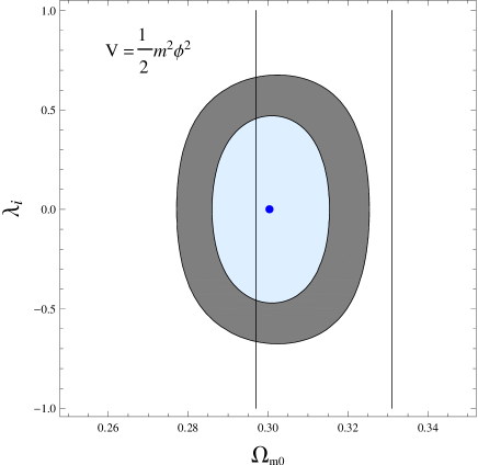
Figure 1: The 1$\sigma$ and 2$\sigma$ confidence regions in the $\lambda_{i}$ - $\Omega_{m0}$ plane for $V=m^{2}\phi^{2}/2$, or $\Gamma=0.5$, constrained by the SN+BAO+CMB+HUB data. The two vertical lines represent the Planck bounds on $\Omega_{m0}$. The thick dot represents the best fit values $\lambda_{i}=0.0008,\Omega_{m0}=0.3003$.

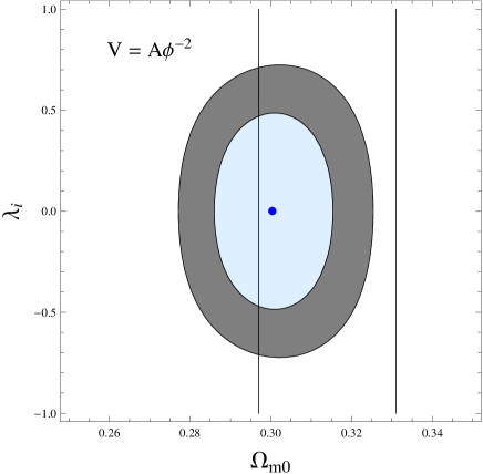
Figure 2: The 1$\sigma$ and 2$\sigma$ confidence regions in the $\lambda_{i}$ - $\Omega_{m0}$ plane for $V=A\phi^{-2}$, or $\Gamma=1.5$, constrained by the SN+BAO+CMB+HUB data. The two vertical lines represent the Planck bounds on $\Omega_{m0}$. The thick dot represents the best fit values $\lambda_{i}=0.0009,\Omega_{m0}=0.3003$.

We note that the likelihood contours for both the potentials look very similar. This indicates that the datasets that we compare with are not able to distinguish between the different potentials under consideration. We have confirmed that the plots of $x,y,\lambda$ and $\Omega_{\phi}$ as functions of $a$, for $\Omega_{m0}=0.3$ show variations between the potentials, but the key parameter that is relevant for comparison of the models with the different datasets is ${\mathcal{H}}(z)$.

In Fig. 3 we plot $\frac{\Delta{\mathcal{H}}_{V}}{{\mathcal{H}}}$ against $z$, where $\Delta{\mathcal{H}}_{V}$ is the difference in ${\mathcal{H}}(z)$ for the two potentials $V\sim\phi^{\pm 2}$ (the denominator corresponds to $V(\phi)\sim\phi^{2}$), for different values of $\lambda_{i}$ with $\Omega_{m0}=0.3$. The relative difference between the two potentials for $\lambda_{i}=1$ reaches a maximum of about $1\%$ and is even smaller for the other considered values of $\lambda_{i}$. The small relative difference is also seen in Fig. 2 of Ref. SenSenSami2010 . This is because in the thawing scenario the field does not roll much in its potential and hence is not sensitive to the form of the potential.

In the inset of Fig. 3 we plot $\frac{\Delta{\mathcal{H}}_{\lambda}}{{\mathcal{H}}}$ against $z$, where $\Delta{\mathcal{H}}_{\lambda}$ is the difference in ${\mathcal{H}}(z)$ for $\lambda_{i}=1,0.2$ for $V\sim\phi^{2}$ (the denominator corresponds to $\lambda_{i}=0.2$), with $\Omega_{m0}=0.3$. Though the relative difference in ${\mathcal{H}}(z)$ is small for different values of $\lambda_{i}$, the data does indicate a difference in the likelihoods for different points in the $\lambda_{i}-\Omega_{m0}$ plane. This is because the SN and CMB datasets disfavor large values of $\lambda_{i}$. The SN data has a large number of datapoints while the CMB shift parameter is very precisely measured and hence these datasets are more sensitive to the variations in $\lambda_{i}$.

Thus far we have presented the results for $V(\phi)\sim\phi^{\pm 2}$. In Fig. 4 we present our results for bounds on $\lambda_{i}$ for different values of $\Gamma$ as would be relevant for other potentials. Our analysis has been carried out for discrete values of $\Gamma$ from 0 to 2, in intervals of 0.25. From Eq. (14), for potentials of the form $V=A\phi^{n}$, where $A$ is taken as real and positive, $n=1/(1-\Gamma)$. Thus Fig. 4 includes potentials with $n=\pm 1,\pm 2,\pm 4$ for $\Gamma=0,2,0.5,1.5,0.75,1.25$ respectively. In addition, we have obtained the bounds for $n=\pm 3$ corresponding to $\Gamma=2/3,4/3$ respectively. For fractional $n$, the form of the potential implies $\phi$ has to be positive and so allowed values of $\lambda_{i}=-nM_{P}/\phi_{i}$ have the opposite sign of $n$. For integer values of $n$, if $n$ is odd, positivity of the dark energy potential energy implies $\phi$ takes positive values. Therefore we presume that $\phi$ takes positive values and project the corresponding values of $\lambda_{i}$ in Fig. 4. To simplify the numerical analysis we have taken $\Omega_{m0}$ to be 0.3. The $1\sigma$ and $2\sigma$ bound on the parameter $\lambda_{i}$ is not very different from what we obtain in case of $V(\phi)\sim\phi^{\pm 2}$. Thus again $|\phi_{i}|>O(M_{P})$. We mention that $\Gamma=1$ corresponds to the case of the exponential potential $V=B\exp({\pm b\,\phi/\phi_{i}})$ and the bound on $\lambda_{i}$ does not give a bound on $\phi_{i}$ due to the presence of the undetermined constant $b$.

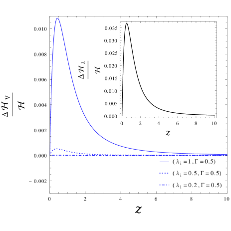
Figure 3: The relative difference in the Hubble parameter, $\frac{\Delta\mathcal{H}_{V}}{\mathcal{H}}$, as a function of redshift $z$ for $V\sim\phi^{\pm 2}$, with $\lambda_{i}$ = 0.2, 0.5 and 1 (from bottom to top) and $\Omega_{m0}=0.3$. The inset shows the relative difference in the Hubble parameter, $\frac{\Delta\mathcal{H}_{\lambda}}{\mathcal{H}}$, as a function of redshift $z$ for $\lambda_{i}$ = 1 and 0.2, for $V\sim\phi^{2}$ and $\Omega_{m0}=0.3$.

We now consider plausible values of $\phi_{i}$ that one may obtain in an inflationary universe by considering a condensate of $\phi$ being generated due to quantum fluctuations during inflation. A light scalar field of mass $m$ ($m\ll H_{I}$, where $H_{I}$ is the Hubble parameter during inflation) will undergo quantum fluctuations during inflation. The fluctuations are given by Eq. (7) of Ref. lindefluc (we presume $H_{I}$ does not vary during inflation)

$$\langle\delta\phi^{2}\rangle=\int_{a_{i}H_{I}}^{aH_{I}}\frac{d^{3}k}{2\pi^{3}}|\delta\phi_{k}|^{2}\\ =\frac{3H_{I}^{4}}{8\pi^{2}m^{2}}\left[1-\exp\left(-\frac{2m^{2}N}{3H_{I}^{2}}\right)\right]$$ (30)

where $N$ is the number of e-foldings of inflation. We consider the case where $m^{2}N\ll H_{I}^{2}$. Then

$$\langle\delta\phi^{2}\rangle=\left(\frac{H_{I}}{2\pi}\right)^{2}N\,.$$ (31)

Ignoring an initial value of $\phi$ at the beginning of inflation, and any potential driven classical evolution, the value of $\phi$ at the end of inflation is

$$\phi_{I}=\pm\sqrt{\langle\delta\phi^{2}\rangle}=\pm\frac{H_{I}}{2\pi}\sqrt{N}$$ (32)

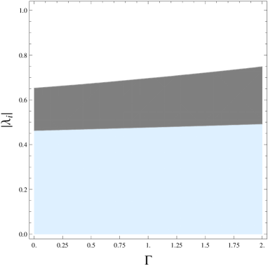
Figure 4: The shaded region shows 1$\sigma$ (blue) and 2$\sigma$(grey) confidence regions in the $|\lambda_{i}|$ - $\Gamma$ plane constrained by the SN+BAO+CMB+HUB data. Discrete values for $\Gamma$ in steps of 0.25 are considered here. $\Gamma=0,0.5,0.75,1.25,1.5,2$ corresponds to $V\sim\phi,\phi^{2},\phi^{4},\phi^{-4},\phi^{-2},\phi^{-1}$ respectively. We have taken $\Omega_{m0}=0.3$. In addition, we have also studied $\Gamma$ values of 2/3 and 4/3, corresponding to $V\sim\phi^{\pm 3}$.

The above discussion is in the context of a quadratic potential, $V=\frac{1}{2}m^{2}\phi^{2}$. For $V=A\phi^{-2}$, and $A\phi^{n}$ considered in Fig. 4, we presume that the potential is very flat during inflation, and so Eq. (31) again describes the evolution of $\phi$.

After inflation $\phi$ will evolve in two ways.

• $\phi$ will evolve classically in its potential $V(\phi)$. Our numerical analysis in Fig. 5 shows that the field does not evolve much between decoupling and the present epoch (less than 10 % for $|\lambda_{i}|<0.7$). We expect its evolution is slower at earlier times. Therefore we may ignore the evolution of $\phi$ from the end of inflation till decoupling. (For a quadratic potential, $m\ll H_{0}\ll H_{I}$ and therefore the assumption $\phi_{i}\sim\phi_{I}$ is obviously justified.)

• After inflation, modes of the $\phi$ field re-enter the horizon (during the radiation and matter dominated eras). These should no longer be considered part of the homogeneous $\phi$ condensate at late time. This can affect $\phi$ by removing $\phi$ fluctuations generated over the last 30-60 e-foldings of (electroweak to GUT scale) inflation. But our constraint on $N$ below will be many orders of magnitude larger so we can ignore this too in our use of Eq. (32).

The above discussion implies that we may take $\phi_{i}\approx\phi_{I}$, i.e., we may assume that the field $\phi$ has not evolved much from inflation till decoupling. From our analysis above we have $|\phi_{i}|>7\times 10^{18}{\rm\,Ge\kern-1.25ptV}$ for $V\sim\phi^{\pm 2}$. Then, from Eq. (32), we get a lower bound on $N$ as

$$N>\frac{2\times 10^{39}{\rm\,Ge\kern-1.25ptV}^{2}}{H_{I}^{2}}$$ (33)

From the Planck bound on the tensor-to-scalar ratio, $H_{I}<9\times 10^{13}{\rm\,Ge\kern-1.25ptV}$ planck-inflation . Therefore we finally obtain

$$N>2\times 10^{11}\,.$$ (34)

A similar bound will apply to the other power law potentials $V\sim\phi^{n}$.

Combining Eq. (33) and the Planck bound on $H_{I}$ we get $H_{I}^{2}/N<3\times 10^{16}{\rm\,Ge\kern-1.25ptV}$. For a quadratic quintessence potential with $m\mbox{\raisebox{-2.58334pt}{~{}$\stackrel{{\scriptstyle<}}{{\sim}}$~{}}}H_{0}\approx 10^{-42}{\rm\,Ge\kern-1.25ptV}$ one sees that our assumption that $m^{2}\ll H_{I}^{2}/N$ is highly feasible.

Ref. ringevaletal also considers a dark energy condensate from quantum fluctuations of the quintessence field during inflation. Their analysis is primarily in the asymptotic limit $m^{2}N\gg H_{I}^{2}$ of Eq. (30). They also consider $m^{2}N\ll H_{I}^{2}$ with an argument similar to that in the paragraph following Eq. (28).

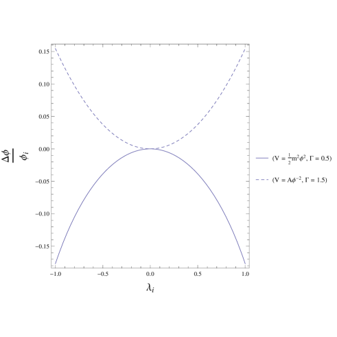
Figure 5: The fractional change in $\phi$ from decoupling to today as a function of $\lambda_{i}$ for $V=m^{2}\phi^{2}/2$ ($\Gamma=0.5$, solid line) and $V=A\phi^{-2}$ ($\Gamma=1.5$, dashed line). We have taken $\Omega_{m0}=0.3$ here. For $|\lambda_{i}|<0.7,$ the fractional change is less than $0.1$, or $10\%$

V Conclusions

In this article we have first numerically solved for the evolution of the quintessence field $\phi$ in thawing models of dark energy for potentials of the form $V\sim\phi^{\pm 2}$ and different values of $\Omega_{m0}$ and $\lambda_{i}=-(M_{P}/V)dV/d\phi=\mp M_{P}/\phi_{i}$, where $\phi_{i}$ is the field value at decoupling. From this we obtain the Hubble parameter $H(z)$, and the luminosity distance and angular diameter distance, as given in Eqs. (15, 19) and (22) respectively. We then relate them to the observations of type Ia supernovae data, the baryon acoustic oscillations data, the cosmic microwave background shift parameter and the observational Hubble parameter data to constrain the values of $\lambda_{i}$ and $\Omega_{m0}$. The likelihood contours for the two potentials looks very similar (due to similar $H(z)$ behaviour) and in both the cases we obtain $|\phi_{i}|>7\times 10^{18}{\rm\,Ge\kern-1.25ptV}$. We extend the analysis to other potentials of the form $V=A\phi^{n}$ and obtain the bound on the initial value of the quintessence field, assuming $\Omega_{m0}=0.3$. Once again, we find that $|\phi_{i}|>O(M_{P})$. We have then argued that $\phi$ does not evolve much between the end of inflation and decoupling and further considered a scenario where the field value at the end of inflation $\phi_{I}$ is due to quantum fluctuations of $\phi$ during inflation. This allows us to use the lower bound on $\phi_{i}\approx\phi_{I}$ to constrain the duration of inflation – the number of e-foldings $N$ is constrained to be greater than $2\times 10^{11}$, for $H_{I}<9\times 10^{13}{\rm\,Ge\kern-1.25ptV}$.

The inflationary paradigm does not stipulate an upper bound on $N$ and so large values of $N$ such as that required above are plausible. Large values of $N$ are more likely in large field inflation models as discussed in Ref. remmen_carroll . However very large values of $N$ can imply a large variation $(\gg M_{P})$ in the inflaton field during inflation which can be problematic if the inflationary scenario constitutes a low energy effective field theory derivable from some Planck scale theory baumannmcallister . On the other hand, one can get a large value of $N$ in eternal inflation scenarios without a large net variation in the inflaton field Guth:2007ng .

- (1) A. G. Riess et al. [Supernova Search Team Collaboration], Astron. J. 116, 1009 (1998) [astro-ph/9805201].
- (2) S. Perlmutter et al. [Supernova Cosmology Project Collaboration], Astrophys. J. 517, 565 (1999) [astro-ph/9812133].
- (3) J. L. Tonry et al. [Supernova Search Team Collaboration], Astrophys. J. 594, 1 (2003) [astro-ph/0305008].
- (4) I. Zlatev, L. M. Wang and P. J. Steinhardt, Phys. Rev. Lett. 82, 896 (1999) [astro-ph/9807002].
- (5) E. J. Copeland, M. Sami and S. Tsujikawa, Int. J. Mod. Phys. D 15, 1753 (2006) [hep-th/0603057].
- (6) M. Li, X. D. Li, S. Wang and Y. Wang, Commun. Theor. Phys. 56, 525 (2011) [arXiv:1103.5870].
- (7) R. R. Caldwell and E. V. Linder, Phys. Rev. Lett. 95, 141301 (2005) [astro-ph/0505494].
- (8) G. Gupta, S. Majumdar and A. A. Sen, Mon. Not. Roy. Astron. Soc. 420, 1309 (2012) [arXiv:1109.4112]
- (9) R. J. Scherrer and A. A. Sen, Phys. Rev. D 77, 083515 (2008) [arXiv:0712.3450].
- (10) N. Suzuki, D. Rubin, C. Lidman, G. Aldering, R. Amanullah, K. Barbary, L. F. Barrientos and J. Botyanszki et al., Astrophys. J. 746, 85 (2012) [arXiv:1105.3470].
- (11) R. Giostri, M. V. d. Santos, I. Waga, R. R. R. Reis, M. O. Calvao and B. L. Lago, JCAP 1203, 027 (2012) [arXiv:1203.3213].
- (12) P. A. R. Ade et al. [Planck Collaboration], Astron. Astrophys. (2014) [arXiv:1303.5076].
- (13) O. Farooq and B. Ratra, Astrophys. J. 766, L7 (2013) [arXiv:1301.5243].
- (14) S. Nesseris and L. Perivolaropoulos, Phys. Rev. D 72, 123519 (2005) [astro-ph/0511040].
- (15) W. Hu and N. Sugiyama, Astrophys. J. 471, 542 (1996) [astro-ph/9510117].
- (16) D. J. Eisenstein et al. [SDSS Collaboration], Astrophys. J. 633, 560 (2005) [astro-ph/0501171].
- (17) S. Sen, A. A. Sen and M. Sami, Phys. Lett. B 686, 1 (2010).
- (18) A. D. Linde, Phys. Lett. B 116, 335 (1982).
- (19) P. A. R. Ade et al. [Planck Collaboration], Astron. Astrophys. 571, A22 (2014) [arXiv:1303.5082 [astro-ph.CO]].
- (20) C. Ringeval, T. Suyama, T. Takahashi, M. Yamaguchi and S. Yokoyama, Phys. Rev. Lett. 105, 121301 (2010) [arXiv:1006.0368].
- (21) G. N. Remmen and S. M. Carroll, Phys. Rev. D 90, 063517 (2014) [arXiv:1405.5538].
- (22) D. Baumann and L. McAllister, arXiv:1404.2601 [hep-th], see Sec. 4.3.
- (23) A. H. Guth, J. Phys. A 40, 6811 (2007) [hep-th/0702178].