Symmetry reduction of turbulent pipe flows

Abstract

We propose and apply a Fourier-based symmetry reduction scheme to remove, or quotient, the streamwise translation symmetry of Laser-Induced-Fluorescence measurements of turbulent pipe flows that are viewed as dynamical systems in a high-dimensional state space. We also explain the relation between Taylor’s hypothesis and the comoving frame velocity $U_{d}$ of the turbulent orbit in state space. In particular, in physical space we observe flow structures that deform as they advect downstream at a speed that differs significantly from $U_{d}$. Indeed, the symmetry reduction analysis of planar dye concentration fields at Reynolds number $\mathfrak{\mathsf{Re}}=3200$ reveals that the speed $u$ at which high concentration peaks advect is roughly 1.43 times $U_{d}$. In a physically meaningful symmetry-reduced frame, the excess speed $u-U_{d}\approx 0.43U_{d}$ can be explained in terms of the so-called geometric phase velocity $U_{g}$ associated with the orbit in state space. The “self-propulsion velocity” $U_{g}$ is induced by the shape-changing dynamics of passive scalar structures observed in the symmetry-reduced frame, in analogy with that of a swimmer at low Reynolds numbers.

1 Introduction

In the last decade, incompressible fluid turbulence in channel flows has been studied as chaotic dynamics in the state space of a high-dimensional system at moderate Reynolds numbers (see, for example, Gibson et al. (2008); Willis et al. (2013)). Here, turbulence is viewed as an effective random walk in state space through a repertoire of invariant solutions of the Navier-Stokes equations (Cvitanović (2013) and references therein). In state space, turbulent trajectories or orbits visit the neighborhoods of equilibria, traveling waves or periodic orbits, switching from one saddle to the other through their stable and unstable manifolds (Cvitanović & Eckhardt (1991), see also Cvitanović et al. (2013)). Recent studies on the geometry of the state space of Kolmogorov flows (Chandler & Kerswell (2013)) and barotropic atmospheric models (Gritsun (2011, 2013)) give evidence that unstable periodic orbits provide the skeleton that underpins the chaotic dynamics of fluid turbulence.

In pipe flows, the intrinsic continuous streamwise translation symmetry and azimuthal symmetry make it difficult to identify invariant flow structures, such as traveling waves or relative equilibria (Faisst & Eckhardt (2003); Wedin & Kerswell (2004)) and relative periodic orbits (Viswanath (2007)), embedded in turbulence. These structures travel downstream with their own mean velocity and there is no unique comoving frame that can simultaneously reduce all relative periodic orbits to periodic orbits and all traveling waves to equilibria. Recently, this issue has been addressed by Willis et al. (2013) using the method of slices (Siminos & Cvitanović (2011); Froehlich & Cvitanović (2012), see also Rowley & Marsden (2000); Rowley et al. (2003)) to quotient group symmetries that reveal the geometry of the state space of pipe flows at moderate Reynolds numbers. Further, Budanur et al. (2015) exploits the ’first Fourier mode slice’ to reduce the $SO(2)$-symmetry in spatially extended systems. In particular, they separate the dynamics of the Kuramoto-Shivasinsky equation into shape-changing dynamics within a quotient or symmetry-reduced space (base manifold) and a one-dimensional (1-D) transverse space (fiber) associated with the group symmetry. This is the geometric structure of a fibration of the state space into a base manifold and transversal fibers attached to it. Thus, the state space is geometrically a principal fiber bundle (e.g. Husemöller (1994),Steenrod (1999),Hopf (1931)): a base or quotient manifold of the true dynamics that is not associated with a drift and has attached transverse fibers of invariant directions.

In this work, we propose a symmetry reduction for dynamical systems with translation symmetries, and apply it to symmetry-reduce the evolution of passive scalars of turbulent pipe flows. The paper is organized as follows. We first discuss the method of comoving frames for pipe flows, also referred to as the method of connections (e.g. Rowley & Marsden (2000)). In particular, we explain the relation of comoving frame velocities to Taylor’s (1938) hypothesis. This is followed by an experimental validation by means of two-dimensional (2-D) Laser-Induced-Fluorescence (LIF) measurements of planar dye concentration fields of turbulent pipe flows. The Fourier-based symmetry reduction scheme is then presented and applied to analyze the acquired experimental data.

2 Comoving frame velocities and Taylor’s hypothesis

Consider an incompressible three-dimensional (3-D) flow field $\mathbf{\mathbf{v_{\mathrm{0}}}}(x,y,z,t)=(U_{0},V_{0},W_{0})$, where $x$ and $z$ are the horizontal streamwise and spanwise directions, and $y$ the vertical axis. The flow satisfies the Navier-Stokes equations with proper no-slip boundary conditions on generic wall boundaries. Consider a 3-D passive scalar field $C_{0}(x,y,z,t)$ advected and dispersed by $\mathbf{v_{\mathrm{0}}}$ in accord with

$$\partial_{t}C_{0}+\mathbf{v_{\mathrm{0}}}\cdot\nabla C_{0}=D_{m}\nabla^{2}C_{0}+f_{0},$$ (2.1)

where $D_{m}$ is the diffusion coefficient, and $f$ accounts for sources and sinks. For the pair $(\mathbf{\mathbf{v_{\mathrm{0}}}},C_{0})$, $\mathbf{\mathbf{v_{\mathrm{0}}}}$ evolves according to the Navier-Stokes equations with no-slip at the wall boundaries and $C_{0}$ evolves according to Eq. (2.1). Assume that solutions to both equations have streamwise translation symmetry. This means that if $\mathbf{(\mathbf{v_{\mathrm{0}}}\mathrm{,\mathit{C}_{0})}}(x,y,t)$ is a solution so is $\mathbf{(\mathbf{v_{\mathrm{0}}}\mathrm{,\mathit{C}_{0})}}(x-\ell,y,t)$ for an arbitrary but fixed shift $\ell$. Hereafter, the translationally invariant Navier-Stokes velocity field $\mathbf{\mathbf{v_{\mathrm{0}}}}$ is not required to be known or given since our approach is based on concentration measurements or observables only.

The presence of translation symmetry allows constructing a symmetry-reduced system, which (depending on construction) is equivalent to observing the original system in a comoving frame $(x-\ell_{d}(t),y,z,t)$, where

$$U_{d}^{(\mathrm{3D})}=\frac{\mathrm{d}\ell_{d}}{\mathrm{d}t}$$ (2.2)

is the comoving frame velocity for 3-D flows. As a first attempt, $U_{d}^{(\mathrm{3D})}$ can be chosen to minimize, on average, the material derivative:

$$\frac{\mathrm{D}C_{0}}{\mathrm{D}t}=\partial_{t}C_{0}+U_{d}^{(\mathrm{3D})}\partial_{x}C_{0},$$ (2.3)

namely

$$\left\langle\left(\partial_{t}C_{0}+U_{d}^{(\mathrm{3D})}\partial_{x}C_{0}\right)^{2}\right\rangle_{x,y,z}$$ (2.4)

is the smallest possible if

$$U_{d}^{(\mathrm{3D})}(t)=-\frac{\left\langle\partial_{t}C_{0}\partial_{x}C_{0}\right\rangle_{x,y,z}}{\left\langle\left(\partial_{x}C_{0}\right)^{2}\right\rangle_{x,y,z}},$$ (2.5)

where the brackets $\left\langle\cdotp\right\rangle{}_{x,y,z}$ denote space average in $x$, $y$ and $z$. In the comoving frame $\left(x-\ell_{d}(t),y,z,t\right)$, with $\ell_{d}(t)=\intop_{0}^{t}U_{d}^{(\mathrm{3D})}(\tau)d\tau$, the passive scalar appears to flow calmly, while still slowly drifting downstream (see, for example, Kreilos et al. (2014) for a study of parallel shear flows). Only when $\frac{\mathrm{D}C_{0}}{\mathrm{D}t}=0$, i.e. the diffusion, source and sink terms are in balance, then the flow is steady in the comoving frame (Krogstad et al. (1998)), for example traveling waves (Faisst & Eckhardt (2003); Wedin & Kerswell (2004)). From (2.1), (2.5) can be written as

$$U_{d}^{(\mathrm{3D})}(t)=\frac{\left\langle U_{0}\left(\partial_{x}C_{0}\right)^{2}+\partial_{x}C_{0}V_{0}\partial_{y}C_{0}+W_{0}\partial_{x}C_{0}\partial_{z}C_{0}-D_{m}\partial_{x}C_{0}\nabla^{2}C_{0}-f_{0}\partial_{x}C_{0}\right\rangle_{x,y,z}}{\left\langle\left(\partial_{x}C_{0}\right)^{2}\right\rangle_{x,y,z}}.$$ (2.6)

Eq. (2.6) reveals that the comoving frame velocity is a weighted average of the local flow velocities, sources and sinks. For periodic boundary conditions the contribution of diffusion processes is null. From (2.5), averaging along the $x$ and $z$ directions only yields the comoving frame vertical velocity profile

$$U_{d}^{(\mathrm{3D})}(y,t)=-\frac{\left\langle\partial_{t}C_{0}\partial_{x}C_{0}\right\rangle_{x,z}}{\left\langle\left(\partial_{x}C_{0}\right)^{2}\right\rangle_{x,z}}.$$ (2.7)

The associated speed $\widehat{U}_{d}$ of a Fourier mode $\widehat{C_{0}}(k_{x},k_{z,},y,t)e^{i(k_{x}x+k_{z}z)}$ then follows as

$$\widehat{U}_{d}(k_{x},k_{z},y,t)=\frac{\mathrm{Re}\left[i\partial_{t}\widehat{C}_{0}(k_{x},k_{z},y,t)\overline{\widehat{C}}_{0}(k_{x},k_{z},y,t)\right]}{k_{x}\left|\widehat{C_{0}}(k_{x},k_{z},y,t)\right|^{2}},$$ (2.8)

where $\overline{\widehat{C_{0}}}$ is the complex conjugate of $\widehat{C_{0}}$, $k_{x}$ and $k_{z}$ are the streamwise and crosswise wavenumbers and $\mathrm{Re}(a)$ denotes the real part of $a$. Note that $\widehat{U}_{d}$ is the same as the convective velocity formulated by Del Álamo & Jimenez (2009) in the context of Taylor’s (1938) abstraction of turbulent flows as fields of frozen eddies advected by the flow. When turbulent fluctuations are small compared to the larger scale flow, they are advected at a speed very close to the time average, or mean flow velocity $U_{m}$ at a fixed point. And their temporal variation at frequency $\omega$ at a fixed point in space can be viewed as the result of an unchanging spatial pattern of wavelength $2\pi/k_{x}$ convecting uniformly past the point at velocity $U_{m}=\omega/k_{x}$. This is Taylor’s hypothesis that relates the spatial and temporal characteristics of turbulence. However, eddies can deform and decay as they are advected downstream and their speed may differ significantly from $U_{d}^{(\mathrm{3D})}$ and $U_{m}.$

In this regard, Del Álamo & Jimenez (2009) concluded that the comoving frame or convective velocity $U_{d}^{(\mathrm{3D})}$ of the largest-scale motion is close to the mean flow speed $U_{m}$, whereas it drops significantly for smaller-scale motions (Krogstad et al. (1998)). Hence, $U_{d}^{(3D)}$ depends on the state of evolution of the flow. For example, it is well known that turbulent motion in channel flows is organized in connected regions of the near wall flow that decelerate and then erupt away from the wall as ejections. These decelerated motions are followed by larger scale connected motions toward the wall from above as sweeps. Krogstad et al. (1998) found that the convection velocity for ejections is distinctly lower than that for sweeps.

To gain more insights into the physical meaning of comoving frame velocities, we performed experiments to trace turbulent pipe flow patterns using non-intrusive LIF techniques (Tian & Roberts (2003)) and discussed in the next section.

2.1 LIF measurements

The experiments were performed in the Environmental Fluid Mechanics Laboratory at the Georgia Institute of Technology. The LIF configuration is illustrated in Fig. (2.1) and a detailed description of the system is given in Tian & Roberts (2003). The tank has glass walls $6.10$ m long × $0.91$ m wide × $0.61$ m deep. The front wall consists of two three-meter long glass panels to enable long unobstructed views. The $5.5$ meter long pipe was located on the tank floor, and the tank was filled with filtered and dechlorinated water. The pipe was transparent Lucite tube with radius $R=2.5\mbox{ cm}$.

The pipe was completely submerged in water to avoid refraction and scattering of the emitted light that would occur at the water-Lucite-air interface along the pipe walls and downstream at the very end of the pipe when the water flows out with curvy streamlines. With this configuration, we enable unique LIF imaging of the flow structures in a round pipe at high flow rate since the pipe discharge is in ambient water instead of air.

The water was pumped into a damping chamber to calm the flow, and then, after passing a rigid polyester filter, it flowed into the pipe. Fluorescent dye solution was continuously injected into the flow through a small hole in the pipe wall upstream of the image capture zone of length $20R$. The solution, a mixture of water and fluorescent dye, is supplied from a reservoir by a rotary pump at a flowrate measured by a precision rotameter. The flow was begun and, after waiting a few minutes for the flow to establish, laser scanning started to record the experiment. To acquire high resolution data, we captured vertical centerline planar fluorescent dye concentration fields $C_{0}(x,y,z=0,t)$ which trace turbulent pipe flow patterns. The pipe Reynolds number $\mathsf{Re}=2U_{b}R/\nu=3200$, where the bulk velocity (discharge divided by the pipe cross sectional area) $U_{b}=6.42\mbox{ cm/s}$ and $\nu$ is the kinematic viscosity of water. As shown in Fig. (2.1), the vertical laser sheet passes through the pipe centerline to focus on flow properties in the central plane ($z=0$). Images of the capture zone ($2R\times 20R=5\times 50\>\mbox{c$m^{2}$}$) were acquired at $50$ Hz for $240$ seconds (see Fig. (2.2)). The vertical and horizontal image sizes are $65\times 622$ pixels for a resolution of $0.0794$ cm/pixel.

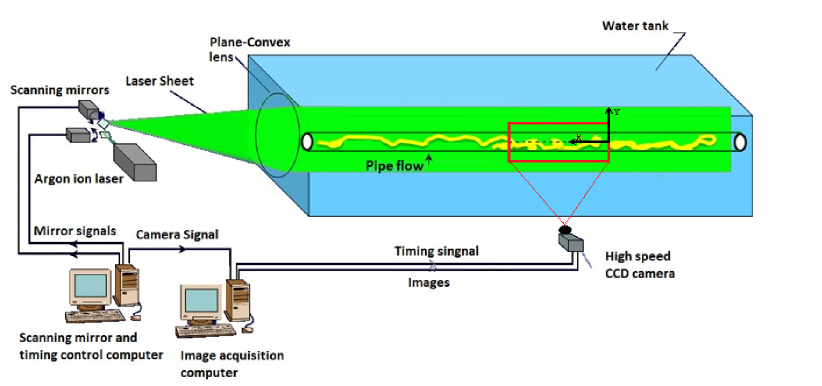
Figure 2.1: Schematic of the LIF system of the Georgia Tech Environmental Fluid Mechanics Laboratory (Tian & Roberts (2003)).

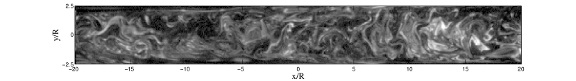
Figure 2.2: LIF experiments: snapshot of the planar fluorescent dye concentration field $C_{0}(x,y,z=0,t)$ tracing turbulent pipe flow patterns at Reynolds number $\mathsf{Re}=3200$ (bulk velocity $U_{b}=6.42\mbox{ cm/s}$, flow from right to left).

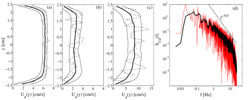
Figure 2.3: LIF experiments: estimated comoving frame, or convective velocity $U_{d}^{(\mathrm{2D})}(y,t)$ using Eq. (2.11): time average profile (solid line), instantaneous profile (dashed line) and its standard deviations about the mean (thin solid line) estimated accounting for (a) all spatial scales of the measured $C$ (max speed$=6.32$ cm/s), (b) small scales (max speed$=2.76$ cm/s), and (c) large scales (max speed$=8.52$ cm/s); (d) observed noisy (red line) and filtered (black line) frequency spectra of the large-scale comoving frame velocity $U_{d}^{(\mathrm{2D})}$ [see Eq. (2.5)]. Pipe radius $R=2.5$ cm.

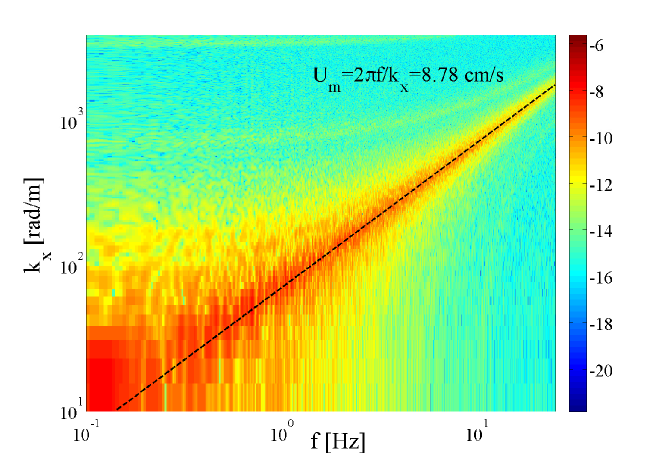
Figure 2.4: Observed log-values of the frequency-wavenumber spectrum $S(k_{x},f)$ of the fluorescent dye concentration $C(x,y=0,t)$ at the pipe centerline. Estimated mean flow velocity $U_{m}=\omega/k_{x}=2\pi f/k_{x}\sim 8.78$ cm/s (dashed line). $U_{m}/U_{b}=1.37$ and bulk velocity $U_{b}=6.42$ cm/s.

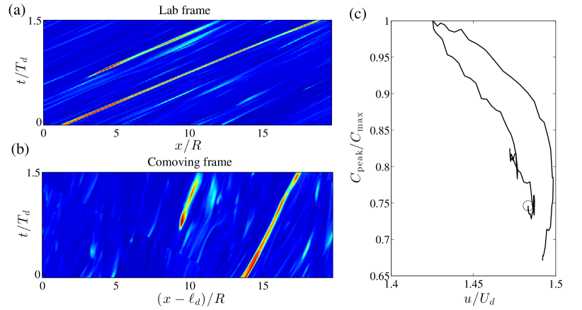
Figure 2.5: LIF experiments: space-time evolution of the dye concentration $C(x,y=0,t)$ at the pipe centerline in the (panel a) lab frame ($x,t)$ and (panel b) comoving frame $(x-x_{d}(t),t)$; (panel c) normalized instantaneous concentration peak intensity $C_{\mathrm{peak}}/C_{\mathrm{max}}$ tracked from the initial time $t/T_{d}=0$ ($\Circle$) as a function of the observed peak speed $u/U_{d}^{(2D)}$, with $C_{\mathrm{max}}$ denoting the observed maximum value of $C$ over the whole data set. $U_{d}\approx$6.34 m/s and $T_{d}=U_{d}/R$.

2.2 Data analysis

The LIF measurements are planar dye concentration fields $C(x,y,t)=C_{0}(x,y,z=0,t)$ in a vertical slice through the pipe centerline. According to Eq. (2.1), at $z=0$, the field $C$ satisfies

$$\partial_{t}C+\mathbf{v_{\mathrm{2D}}}\cdot\nabla_{xy}C=D_{m}\nabla_{xy}^{2}C+f,$$ (2.9)

where $\nabla_{xy}=\left(\partial_{x},\partial_{y}\right)$ and $\mathbf{v}_{\mathrm{2D}}=(U,V)=(U_{0}(x,y,z=0,t),V_{0}(x,y,z=0,t))$ are the in-plane gradient and flow within the 2D slice and the source

$$f(x,y,t)=-W_{0}(x,y,z=0,t)\partial_{z}C+D_{m}\left.\partial_{zz}C\right|_{z=0}+f_{0}(x,y,z=0,t)$$

accounts for the out-of-plane transport and diffusion and in-plane source/sinks. The associated in-plane comoving frame, or convective, velocity $U_{d}^{(2D)}$ can be estimated from the measured field $C(x,y,t)$ using Eq. (2.5), where the average is performed only in the $x$ and $y$ directions, that is

$$U_{d}^{(\mathrm{2D})}(t)=-\frac{\left\langle\partial_{t}C\partial_{x}C\right\rangle_{x,y}}{\left\langle\left(\partial_{x}C\right)^{2}\right\rangle_{x,y}}=\frac{\left\langle\widetilde{U}\left(\partial_{x}C\right)^{2}+\widetilde{V}\partial_{x}C\partial_{y}C-D_{m}\partial_{x}C\nabla_{xy}^{2}C-f\partial_{x}C\right\rangle_{x,y}}{\left\langle\left(\partial_{x}C\right)^{2}\right\rangle_{x,y}}.$$ (2.10)

Clearly, this depends on the in-plane flow and out-of-plane sources/sinks. Similarly, the in-plane comoving frame, or convective, velocity profile $U_{d}^{(\mathrm{2D})}(y,t)$ follows from Eq. (2.7) averaging only in the $x$ direction,

$$U_{d}^{(\mathrm{2D})}(y,t)=-\frac{\left\langle\partial_{t}C\partial_{x}C\right\rangle_{x}}{\left\langle\left(\partial_{x}C\right)^{2}\right\rangle_{x}}.$$ (2.11)

For example, Fig. (2.3) shows the comoving frame velocity profiles computed from Eq. (2.11) including (Panel $a$) all spatial scales of the measured $C$, (Panel $\mathit{b}$) the small scales (wavelengths $L_{x}<0.2R$, $L_{y}<0.2R$) and (Panel $c$) the large scales ($L_{x}>2R$, $L_{y}>0.4R$). Clearly, the small scales advect more slowly than the large scales, in agreement with Krogstad et al. (1998). Moreover, the maximum comoving frame velocity of the large scales ($=8.52\mbox{ cm/s}$) is close to the centerline mean flow speed (=$8.78$ cm/s) estimated from the frequency-wavenumber spectrum of $C(x,y=0,t)$ [see Figure (2.4)]. Further, the frequency spectrum of the comoving frame velocity $U_{d}(t)$ estimated from Eq. (2.10) accounting for large scales only is also shown in Panel $d$ of Fig. (2.3). It decays approximately as $f^{-5/3}$, indicating that Taylor’s hypothesis is approximately valid, possibly due to the non-dispersive behavior of large scale motions.

In the fixed frame $(x,t)$, the space-time evolution of the measured dye concentration $C(x,y=0,t)$ on the pipe centerline is shown in Panel $a$ of Figure (2.5). The associated evolution in the comoving frame $\left(x-\ell_{d}(t),t\right)$ is shown in Panel $b$ of the same Figure. The shift $\ell_{d}$ is computed by numerically integrating $U_{d}^{(\mathrm{2D})}$ in time, which is estimated from Eq. (2.11) accounting for all spatial scales of $C$. Note the shape-changing dynamics of the passive scalar structures, which still experience a drift in the comoving frame. Moreover, a slowdown or deceleration is observed in the dye concentration peaks, possibly related to the above mentioned turbulent flow ejections. This is clearly seen in Panel $c$ of Figure (2.5), which depicts the normalized instantaneous peak concentration $C_{\mathrm{peak}}$ (normalized to $C_{\mathrm{max}}$) as a function of the associated peak speed $u$ (normalized to $U_{d}^{(\mathrm{2D})}$), with $C_{\mathrm{max}}$ denoting the maximum value of $C$ over the whole 2-D data set. Further, the peak speed $u$ is approximately 40% larger than the comoving frame velocity, which is roughly constant during the event ($U_{d}^{(\mathrm{2D})}=6.32\pm 0.22$ cm/s). Note that in oceanic wave groups, large focusing crests tend to slow down as they evolve within the group, as a result of the natural wave dispersion of unsteady wave trains (Banner et al. (2014); Fedele (2014b, a)). Thus, we argue that the observed slowdown of the passive scalar peaks may be due to the wave-like dispersive nature of small-scale turbulent structures.

Drawing from differential geometry, the observed excess speed $u-U_{d}^{(\mathrm{2D})}$ of concentration peaks is explained in terms of geometric phases.

3 Geometric phases

A classical example in which geometric phases arise is the transport of a vector tangentially on a sphere. The change in the vector direction is equal to the solid angle of the closed path spanned by the vector and it can be described by Hannay’s angles (Hannay (1985)). The rate at which the angle, or geometric phase, changes in time is the geometric phase velocity. In physics, the rotation of Foucault’s pendulum can be also explained by means of geometric phases. Pancharatnam (1956) discovered their effects in polarized light, and later Berry (1984) for quantum-mechanical systems.

Consider another example drawn from classical mechanics. The dynamics of a spinning body in a dissipationless media admits rotational symmetry with respect to the axis of rotation. The associated angular, or geometric phase velocity $\Omega$ follows from conservation of angular momentum $I\Omega^{2}$, where $I$ is the moment of inertia. Clearly, $\Omega$ can vary in time if the body shape deforms to induce changes in $I$. Since the body shape and its deformations are usually known, the rotation speed depends only on how the shape deforms. Indeed, in the frame rotating at the speed $\Omega$, we only observe the body shape-changing dynamics and the rotational symmetry is “removed” or quotiented out. We label this special frame as symmetry-reduced since in a fixed laboratory frame we cannot distinguish between the body deformation and spinning motions.

In fluid mechanics, the motion of a swimmer at low Reynolds numbers can also be explained in terms of geometric phase velocities (Shapere & Wilczek (1989)). In this case, the comoving frame velocity is null since inertia is neglected and the swimmer’s velocity is uniquely determined by the geometry of the sequence of its body’s shapes, which lead to a net translation, i.e. the geometric phase. In a fixed laboratory frame we observe the swimmer drifting as its body’s shape varies in time, but it is hard to distinguish between the two types of motions. In the symmetry-reduced frame moving with the swimmer we only observe its body deformations and translation symmetry is quotiented out.

In wave mechanics, the recently noticed slowdown effect of crests of oceanic wave groups can be explained in terms of geometric phase velocities (Fedele (2014a); Banner et al. (2014)).

In the abovementioned cases, the associated governing equations are linear and the shape deformations are known or assumed a priori. Indeed, in quantum-mechanical systems their shape depends on the eigenfunctions of the Schrodinger operator (Berry (1984)). Shapere & Wilczek (1989) considered the eigenfunctions of the Stokes operator to describe the swimmer’s shape. Fedele (2014a) considered the special class of Gaussian envelopes to study the qualitative dynamics of realistic ocean wave groups.

In turbulent pipe flows, fluctuating coherent structures advect downstream at a speed that depends on both their intrinsic properties such as inertia, and on the way their “shape” varies or deforms in time. However, we don’t know a priori their shape as the Navier-Stokes equations are nonlinear and one cannot rely on an eigenfunction expansion to model shapes. Clearly, one can use the eigenfunctions of the linearized Navier-Stokes operator or define a special flow given by the superposition of patches of constant vorticity whose boundaries change in time according to given shape modes. However, these are just approximations or simplifications of the more complex turbulent flows.

In general, the speed of coherent structures includes not only the comoving frame velocity, which accounts primarily for their inertia, but also a geometric component. This can be interpreted as a “self-propulsion” velocity induced by the shape-changing deformations of the flow structures similar to that of a swimmer at low Reynolds numbers (Shapere & Wilczek (1989)).

To unveil the “shape of turbulence” we need to quotient out the translation symmetry. This can be achieved, for example, by means of a physically meaningful slice representation of the quotient space (Budanur et al. (2015); Cvitanović et al. (2012)). Slicing should provide a symmetry-reduced frame from which one observes the shape-changing dynamics of coherent structures without drift. The relative velocity between the comoving and symmetry-reduced frame is the geometric phase velocity.

Clearly, in the previous section we have seen that the comoving frame velocity of pipe flows has the physical meaning of a convective speed. The geometric phase velocity, on the other hand, depends on an arbitrary definition of the symmetry-reduced frame. Different slice representations yield different symmetry-reduced frames, as we will show later. Finding a physically meaningful symmetry-reduced frame from which one observes the shape of turbulence is still an open problem.

In the following, we first present a symmetry reduction scheme to quotient translation symmetry using slice representations, and then we apply it to symmetry-reduce the LIF data of turbulent pipe flows presented in the previous section.

4 Symmetry reduction via slicing

As an application, we focus on the desymmetrization of the average in-plane concentration field $c(x,t)=\left\langle C(x,y,t)\right\rangle{}_{y}$. It is convenient to express $c$ by means of the truncated Fourier series

$$\begin{array}[t]{c}c(x,t)=c_{0}(t)+\frac{1}{2}\sum_{m=1}^{N}z_{m}(t)\exp\left(imk_{x}x\right)+c.c.=\\ \\ c_{0}(t)+\sum_{m=1}^{N}\left|z_{m}(t)\right|\cos\left(mk_{0}x+\theta_{m}(t)\right),\end{array}$$ (4.1)

where $c_{0}(t)$ is the mean, $z_{m}=\left|z_{m}\right|\exp(i\theta_{m})$ is the complex Fourier amplitude with phase $\theta_{m}$, $k_{0}=2\pi/L_{0}$ is a minimum possible wavenumber for the domain length $L_{0}$ of interest, and the index $m$ runs from $1$ to $N$. The mean $c_{0}$ is invariant under the group action, but its evolution is coupled to that of the fluctuating component of $c$. This depends on the evolution of the vector $\mathbf{z}(t)=\{z_{m}\}=(z_{1},...z_{N})$ of Fourier components of $c$ and those of the translationally invariant Navier-Stokes velocity field $\mathbf{v}$, denoted by the vector $\hat{\mathbf{v}}$. The velocity field is not required to be given or known because the proposed symmetry reduction can be applied to concentration measurements only.

The coupled dynamics of $c_{0}$ and $\mathbf{z}$ can be derived by averaging the governing equation (2.9) in the $y$ direction, applying flow boundary conditions and projecting onto Fourier basis. Without losing generality, we can write

$$\left\{\begin{array}[]{c}\frac{d\mathbf{z}}{dt}=\mathcal{N_{\mathrm{1}}}(c_{0},\mathbf{z},\mathbf{\hat{\mathbf{v}}})\\ \\ \frac{dc_{0}}{dt}=\mathcal{N_{\mathrm{2}}}(c_{0},\mathbf{z},\mathbf{\hat{\mathbf{v}}})\end{array}\right.,$$ (4.2)

where $\mathcal{N_{\mathrm{1}}}$ and $\mathcal{N_{\mathrm{2}}}$ are appropriate nonlinear operators of their arguments and both are invariant under translation symmetry, viz. $\mathcal{N_{\mathrm{k}}}(c_{0},g_{\ell}(\mathbf{z}),\mathbf{\mathrm{\mathit{g_{\ell}}}\hat{\mathbf{v}}})=g_{l}\mathcal{N_{\mathrm{k}}}(c_{0},\mathbf{z},\mathbf{\hat{\mathbf{v}}})$. The orbit $\mathbf{z}$ wanders in the state space $\mathcal{P}\in\mathbb{C^{\mathrm{\mathit{N}}}}$, and the one-parameter group orbit $g_{\ell}(\mathbf{z})$ of $\mathbf{z}$ is the subspace

$$g_{\ell}(\mathbf{z})=\left\{\mathbf{w}\in\mathbb{C^{\mathit{N}}}:\mathbf{w}=\{z_{m}\exp(imk_{0}\ell)\},\>\forall\ell\in\mathbb{R}\right\},$$ (4.3)

where the length $\ell$ is the drift. For a non-vanishing Fourier mode $z_{j}$, the symmetry-reduced or desymmetrized orbit $\mathbf{Z}(t)$ is defined by the complex components

$$\mathbf{Z}=\Pi_{j}(\mathbf{z})=\{Z_{m}\}=\left\{z_{m}\left(\frac{\bar{z}_{j}}{\left|z_{j}\right|}\right)^{m/j}\right\}=\left\{\left|z_{m}\right|\exp(i\phi_{m})\right\},$$ (4.4)

where the phases

$$\phi_{m}=\theta_{m}-\frac{m\theta_{j}}{j}.$$ (4.5)

Note that $Z_{j}=\left|z_{j}\right|$ is real and $\mathbf{Z}\in\mathbb{C^{\mathrm{\mathit{\mathit{N\mathrm{-1}}}}}}$. For $j=1$, the reduction scheme yields the ’first Fourier mode slice’ proposed in Budanur et al. (2015). The scalar field $c_{D}$ in the symmetry-reduced frame follows from (4.1) as

$$c_{D}(x,t)=c_{0}(t)+\sum_{m=1}^{N}\left|z_{m}\right|\cos\left(mk_{0}x+\phi_{m}\right).$$ (4.6)

It is straightforward to check that any translated copy of $c(x+\ell,t)$ corresponds to a unique $c_{D}$. Indeed, the associated Fourier phases $\phi_{m}$ in (4.5) are invariant under the change $\theta_{m}\rightarrow\theta_{m}+m\ell.$ In mathematical terms, the map $\Pi_{j}$ projects an element $\mathbf{z}=\{z_{m}\}$ of $\mathcal{P}$ and all the elements of its group orbit $g_{\ell}\mathbf{\mathrm{(}z\mathrm{)}}$ into the same point $\mathbf{Z}=\Pi_{j}(\mathbf{z})$ of the quotient space $\mathcal{M}=\mathcal{P}/g_{\ell}\in\mathbb{C^{\mathrm{\mathit{N-1}}}}$, i.e. $\Pi_{j}(\mathbf{z})=\Pi_{j}(g_{\ell}(\mathbf{z}))$. Note that $\mathcal{M}$ has one dimension less than the original space since we have ’removed’ translation symmetry. Indeed, $\mathcal{M}$ is defined as a manifold of $\mathbb{C}^{\mathrm{\mathit{N}}}$ that satisfies $\mathrm{Im}(z_{j})=0$.

For $j>1$, the presence of complex roots of $z_{m}$ requires care in computing the components $Z_{m}$ in (4.4). In particular, we define a slice as a subregion of the original state space $\mathcal{P}$ whose elements are mapped onto the quotient space $\mathcal{M}$ via the projection map $\Pi_{j}$. Slicing a state space is in general not unique. In this work, we consider the Fourier slice $S_{j}$ of $\mathcal{P}$ defined as

$$S_{j}=\left\{\mathbf{z}\in\mathbb{C^{\mathit{N}}}:z_{j}\neq 0\right\},$$ (4.7)

which is a region of $\mathbb{C}^{\mathrm{\mathit{N}}}$ delimited by, but not including, the border of $S_{j}$, i.e. the hyperplane $z_{j}=0$. $S_{j}$ can be divided in $j$ wedge-shaped subregions based on the values of the phase $\theta_{j}$ of $z_{j}$ as

$$S_{j}=\bigcup_{k=0}^{j-1}S_{j,k},$$ (4.8)

where the subslice $S_{j,k}$ is the wedge domain defined as

$$S_{j,k}=\left\{\mathbf{z}\in\mathbb{C^{\mathit{N}}}:z_{j}\neq 0\,\,\,\mathrm{and}\,\,\,\frac{2\pi}{j}k<\theta_{j}<\frac{2\pi}{j}(k+1)\right\}.$$ (4.9)

The division into subslices is necessary because the phases $\phi_{m}$ of $Z_{m}$ in Eq. (4.5) jump by $2\pi/j$ each time the orbit $z_{j}$ winds around the origin of the complex plane crossing the branch cut $\left\{\mathrm{Re}(z_{j})\in(0,-\infty)\,\right\}$. Thus, $\Pi_{j}$ maps elements of $\mathcal{P}$ into any of the $k$ subslices $S_{j,k}$. As $z_{j}$ winds around the origin, a different $S_{j,k}$ has to be chosen to have continuity of the phases $\phi_{m}$ of $Z_{m}$. Tracking the winding number $\mathrm{Im}\ointop\frac{\mathrm{d}z_{j}}{z_{j}}$ signals when one must switch to a different subslice. In a more practical way, a jump-free symmetry-reduced orbit $\mathbf{Z}$ is obtained by first unwrapping the phase $\theta_{j}$ of $z_{j}$ and then computing $Z_{m}$ by means of Eqs. (4.4) and (4.5). As a result, $\Pi_{j}$ is defined on the slice $S_{j}$ (see Eq. (4.7)).

Within the quotient space $\mathcal{M}$, after $j$ cycles are completed relative equilibria reduce to equilibria and relative periodic orbits (RPOs) reduce to periodic orbits (POs). Indeed, after one cycle the projected orbit drifts by $2\pi/(jk_{0})$ in physical space, and we refer to it as modulo-$2\pi/j$ periodic orbit (MPO). Each RPO and its shifted copies are uniquely mapped to an MPO in the quotient space since the symmetry reduction is well defined. Clearly, an ergodic trajectory, which temporarily visits neighborhoods of RPOs in full space may experience on average no drift in the desymmetrized or quotient space if the slice $j$ is properly chosen, as will be shown later on. The practical and easy choice would be the first Fourier slice $S_{1}$. However, a good reduction requires the amplitude of $z_{j}$ to be dominant in comparison to the other Fourier components. Indeed, in general as $z_{j}$ lingers near zero, the orbit wanders near the border of the slice $S_{j}$. As a result, the map $\Pi_{j}$ becomes singular since the phase $\theta_{j}$ is undefined (see, for example, Budanur et al. (2015)). A different slice can then be chosen and the slices’ borders can be adjoined via ridges into an atlas that spans the state space region of interest (Cvitanović et al. (2012)).

The choice of the Fourier slice $S_{j}$ to quotient out the translation symmetry is entirely arbitrary. Different slices yield different symmetry-reduced frames in which the concentration field may appear distorted. As an example, consider the state space to be an infinitely long vertical cylinder with its vertical lines fibers of the principal bundle (e.g. Husemöller (1994),Steenrod (1999)). Each fiber can be associated with a single point in the quotient space. If we slice the cylinder transversally by a plane, the quotient space is an ellipse, or circle if the plane is orthogonal to the fibers. Of course, we can also slice the cylinder with a curved surface and the slice is a warped ellipse. Clearly, different slices are equivalent since slanted/warped ellipses and circles can be mapped into each other.

Thus, what is the best Fourier slice representation of turbulent pipe flows? We argue that a proper choice of the Fourier slice should provide a physically meaningful symmetry-reduced frame in which the shape-changing dynamics of coherent structures is observed without drift. In this case, the observed drift in the comoving frame is explained by means of geometric phases (see panel $b$ of Fig. (2.5)). For our LIF measurements we need to resort to higher order Fourier slices, as we will show below.

4.1 Dynamical and geometric phases

From (4.4), the action of the map $\Pi_{j}$ is to shift the orbit $\mathbf{\mathit{\mathbf{z}}}(t)=\left\{z_{m}(t)\right\}$ in $\mathcal{P}$ by an amount

$$\ell_{s}=-\frac{\theta_{j}}{k_{0}j},\qquad j\geq 1,$$ (4.10)

and the resulting desymmetrized or sliced orbit

$$\mbox{$\mathit{\mathbf{\mathrm{\mathbf{Z}}}}$}(t)=g_{-\ell_{s}}(\mathrm{\mathrm{\mbox{$\mathbf{z}$}}})=\left\{Z_{m}(t)\right\}$$

has Fourier components

$$Z_{m}=z_{m}\exp(-imk_{0}\ell_{s}),\qquad m=1,...N.$$

Note that the desymmetrized orbit $\mathbf{Z}=g_{-\ell_{s}}(\mathbf{z})$ does not satisfy the same dynamical equation (4.2) for $\mathbf{z}$, i.e. $\frac{\mathrm{d}\mathbf{z}}{\mathrm{d}t}=\mathcal{N_{\mathrm{1}}}(\mathbf{z})$. Indeed, (see appendix)

$$\frac{\mathrm{d}\mathbf{Z}}{\mathrm{d}t}+\frac{\mathrm{d}\ell_{s}}{\mathrm{d}t}T(\mathbf{Z})-\mathcal{N_{\mathrm{1}}}(\mathbf{Z})=0,$$ (4.11)

where

$$T(\mathbf{Z})=(g_{\ell}^{-1}\partial_{\ell}g)(\mathbf{Z})=\{imk_{0}Z_{m}\}$$ (4.12)

is the tangent space to the group orbit at $\mathbf{Z}$ (see, for example, Cvitanović et al. (2013)).

It is well known that the total drift $\ell_{s}$ is the sum of dynamical ($\ell_{d}$) and geometric ($\ell_{g}$) phase drifts (Simon (1983); Samuel & Bhandari (1988))

$$\ell_{s}=\ell_{d}+\ell_{g},$$ (4.13)

where

$$\ell_{d}=\int_{0}^{t}U_{d}\mathrm{d}\tau,\qquad\qquad\ell_{g}=\int_{0}^{t}U_{g}\mathrm{d}\tau.$$ (4.14)

Here, we have defined the associated dynamical ($U_{d}$) and geometric ($U_{g}$) phase velocities and the total drift speed follows as

$$U_{s}=\frac{d\ell_{s}}{dt}=U_{d}+U_{g}.$$ (4.15)

The decomposition in dynamical and geometric components of the drift $\ell_{s}$ and associated velocity follows from the condition of transversality of the symmetry-reduced trajectory $\mathbf{Z}$ to the group orbit $g_{\ell_{s}}(\mathbf{Z})$, that is $d\mathbf{Z}/dt$ is transversal to the group orbit tangent $T(\mathbf{\mathbf{Z}})$ (Viswanath (2007); Cvitanović et al. (2013)). Indeed, multiply both members of Eq. (4.11) by $\overline{T(\mathbf{Z})}$ as

$$\overline{T(\mathbf{\mathbf{Z}})}\cdot\frac{\mathrm{d}\mathbf{Z}}{\mathrm{d}t}+\frac{\mathrm{d}\ell_{s}}{\mathrm{d}t}\left|T(\mathbf{Z})\right|^{2}-\overline{T(\mathbf{Z})}\mathcal{\cdot N_{\mathrm{1}}}(\mathbf{Z})=0,$$ (4.16)

where

$$\mathbf{a}\cdot\mathbf{b}=\overline{a}_{p}W_{pq}b_{q}$$ (4.17)

is a weighted scalar product of two vectors with weights $W_{pq}=\overline{W}_{qp}$. In this work we will use the standard scalar product and the group orbit is sliced orthogonally, i.e. $W_{pq}=\delta_{pq}$ where $\delta_{pq}$ is the Kronecker symbol.

The rate of change of the total drift $\ell_{s}$ is a real number and it follows from the real part of Eq. (4.16) as

$$U_{s}=\frac{\mathrm{d}\ell_{s}}{\mathrm{d}t}=\underset{\mathrm{dynamic}}{\underbrace{\frac{\mathrm{Re}\left(\overline{T(\mathbf{Z})}\mathcal{\cdot N_{\mathrm{1}}}(\mathbf{Z})\right)}{\left|T(\mathbf{Z})\right|^{2}}}+}\underset{\mathrm{geometric}}{\underbrace{\frac{\mathrm{-Re}\left(\overline{T(\mathbf{Z})}\cdot\frac{\mathrm{d}\mathbf{Z}}{\mathrm{d}t}\right)}{\left|T(\mathbf{Z})\right|^{2}}}}.$$ (4.18)

Here,

$$U_{d}=\frac{\mathrm{d}\ell_{d}}{\mathrm{d}t}=\frac{\mathrm{Re}\left(\overline{T(\mathbf{Z})}\mathcal{\cdot N_{\mathrm{1}}}(\mathbf{Z})\right)}{\left|T(\mathbf{Z})\right|^{2}}.$$ (4.19)

is the so-called dynamical phase velocity (Simon (1983); Samuel & Bhandari (1988)). Since $\overline{T(\mathbf{Z})}\mathcal{\cdot N}_{\mathrm{1}}(\mathbf{Z})$ and $\left|T(\mathbf{Z})\right|^{2}$ are invariant under translation symmetry, $\ell_{d}$ can also be determined replacing $\mathbf{Z}$ with the orbit $\mathbf{z}$ in $\mathcal{P}$, which is usually known or observable in applications. Indeed, from (4.19) and (4.2)

$$U_{d}=\frac{\mathrm{Re}\left(\overline{T(\mathbf{z})}\mathcal{\cdot N_{\mathrm{1}}}(\mathbf{z})\right)}{\left|T(\mathbf{z})\right|^{2}}=\frac{\mathrm{Re}\left(\overline{T(\mathbf{z})}\cdot\frac{\mathrm{d}\mathbf{z}}{\mathrm{d}t}\right)}{\left|T(\mathbf{z})\right|^{2}}.$$ (4.20)

It is straightforward to show that $U_{d}$ depends on the evolution of the concentration field $c$ in the fixed laboratory frame $(x,t)$ associated with the orbit $\mathbf{z}$ in $\mathcal{P}$. Indeed, since

$$\left\langle\left(\partial_{x}c\right)^{2}\right\rangle_{x}=\sum_{m=1}^{N}m^{2}k_{0}^{2}\left|z_{m}\right|^{2}=\left|T(\mathbf{z})\right|^{2}$$ (4.21)

and

$$\mathrm{\mathit{\left\langle\partial_{t}c\partial_{x}c\right\rangle_{x}}}=\mathrm{Re}\sum_{m=1}^{N}imk_{0}\overline{z_{m}}\frac{\mathrm{d}z_{m}}{\mathrm{d}t}=\mathrm{-Re}\left(\overline{T(\mathbf{z})}\cdot\frac{\mathrm{d}\mathbf{z}}{\mathrm{d}t}\right),$$ (4.22)

it follows that

$$U_{d}=-\frac{\left\langle\partial_{t}c\partial_{x}c\right\rangle_{x}}{\left\langle\left(\partial_{x}c\right)^{2}\right\rangle_{x}}.$$ (4.23)

Thus, the dynamical phase velocity $U_{d}$ is the 1-D comoving frame, or convective, speed similar to that defined for 2-D and 3-D concentration fields (see Eqs. (2.10) and (2.5), respectively). Clearly, $U_{d}$ also follows by minimization of the spatial mean of the material derivative of $c$ as in Eq. (2.4). Further, from (4.18) we define the geometric phase velocity as

$$U_{g}=\frac{\mathrm{d}\ell_{g}}{\mathrm{d}t}=\frac{\mathrm{Re}\left(\overline{T(\mathbf{Z})}\cdot\frac{\mathrm{d}\mathbf{Z}}{\mathrm{d}t}\right)}{\left|T(\mathbf{Z})\right|^{2}}.$$ (4.24)

Note that $U_{g}$ and $U_{d}$ in (4.23) are not the same since $\frac{\mathrm{d}\mathbf{Z}}{\mathrm{d}t}\neq\frac{\mathrm{d}\mathbf{z}}{\mathrm{d}t}$ (see Eqs. (4.2) and (4.11)). Further, in contrast to the dynamical $U_{d}$, the geometric $U_{g}$ cannot be related to the evolution of the concentration field $c$ in the fixed laboratory frame $\left(x,t\right)$; it depends only on the shape-changing evolution of the desymmetrized field $c_{D}$ (see Eq. (4.6)) in the symmetry-reduced frame $\left(x-\ell_{d}-\ell_{g},t\right)$. Here, we recall that $c_{D}$ is associated with the desymmetrized orbit $\mathbf{Z}$ in the quotient space $\mathcal{M}$, or base manifold. Indeed, Eq. (4.24) can be written as

$$U_{g}=-\frac{\left\langle\partial_{t}c_{D}\partial_{x}c_{D}\right\rangle_{x}}{\left\langle\left(\partial_{x}c_{D}\right)^{2}\right\rangle_{x}},$$ (4.25)

where we have used Eqs. (4.21,4.22) replacing $\mathbf{z}$ with $\mathbf{Z}$. Clearly, the geometric phase velocity depends on the arbitrary choice of the Fourier slice $S_{j}$. Indeed, different slices yield different desymmetrized concentration fields $c_{D}$, as discussed later. Further, different scalar products in Eq. (4.17) could be used to filter out the contribution of large or small flow scales leading to different slice representations. As mentioned above, in this work we only consider the standard scalar product and all flow scales are accounted for.

The comoving orbit

$$\mathbf{Z}_{d}(t)=g_{-\ell_{d}}(\mathbf{z})$$ (4.26)

is the orbit seen from a comoving frame drifting at the speed $U_{d}$. In physical space it corresponds to an evolution of the dye concentration in the comoving frame $\left(x-\ell_{d},t\right)$. Note that in general $\ell_{d}(t)$ is time varying, and constant only for traveling waves. Clearly, the dynamical drift $\ell_{d}$ increases with the time spent by the trajectory $\mathbf{z}(t)$ to wander around $\mathcal{P}$. The geometric drift $\ell_{g}$ instead depends upon the path $\Gamma=\{Z_{n}(t)\}$ associated with the desymmetrized orbit $\mathbf{Z}(t)$ in the quotient space. Indeed,

$$\ell_{g}(t)=\int_{0}^{t}U_{g}\mathrm{d}\tau=-\int_{0}^{t}\frac{\mathrm{Re}\left(\overline{T(\mathbf{Z})}\cdot\frac{\mathrm{d}\mathbf{Z}}{\mathrm{d}\tau}\right)}{\left|T(\mathbf{Z})\right|^{2}}\mathrm{d}\tau=-\int_{\Gamma}\frac{\mathrm{Re}\left(\overline{T(\mathbf{Z})}\mathrm{\cdot d}\mathbf{Z}\right)}{\left|T(\mathbf{Z})\right|^{2}}.$$ (4.27)

The desymmetrized orbit $\mathbf{Z}$ is obtained by further shifting the comoving orbit $\mathbf{Z}_{d}$ in Eq. (4.26) by the geometric drift $\ell_{g}$ as

$$\mathbf{Z}=g_{-\ell_{g}}(\mathbf{Z}_{d})=g_{-\ell_{d}-\ell_{g}}(\mathbf{z}).$$ (4.28)

Different slice representations yield different symmetry-reduced frames $(x-\ell_{d}-\ell_{g},t)$ from which one observes distorted shape-changing dynamics of the dye concentration field. Only relative equilibria or traveling waves have null geometric phase, since their shape is not dynamically changing in the base manifold as they reduce to equilibria. The geometric drift $\ell_{g}$ and associated speed $U_{g}$ can be indirectly computed from Eqs. (4.13,4.15) as $\ell_{g}=\ell_{s}-\ell_{d}$ and $U_{g}=U_{s}-U_{d}$ respectively. The pairs $(\ell_{s}$,$U_{s}=d\ell_{s}/dt)$ and $(\ell_{d}=\int_{0}^{t}U_{d}\mathrm{d}\tau,U_{d})$ are easily estimated from concentration measurements.

The Fourier slice should be properly chosen to provide a physically meaningful symmetry-reduced frame, as discussed in the next section.

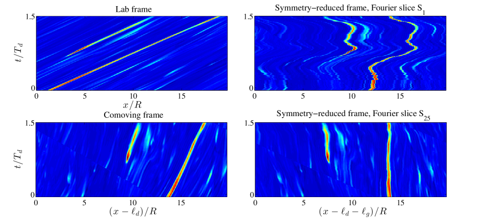
Figure 4.1: Symmetry reduction of LIF measurements: space-time evolution of a passive scalar structures; (left panels) measured concentration $C(x,y=0,t)$ at the pipe centerline in the (left-top) fixed frame, (left-bottom) comoving frame $\left(x-\ell_{d},t\right)$, (right panels) symmetry-reduced frame $\left(x-\ell_{d}-\ell_{g},t\right)$ using Fourier slices (right-top) $S_{1}$ and (right-bottom) $S_{25}$; time average $\overline{U}_{d}\approx 6.74$ cm/s, $\overline{U}_{g}\approx 0.4U_{d}$ and $T_{d}=\overline{U}_{d}/R$.

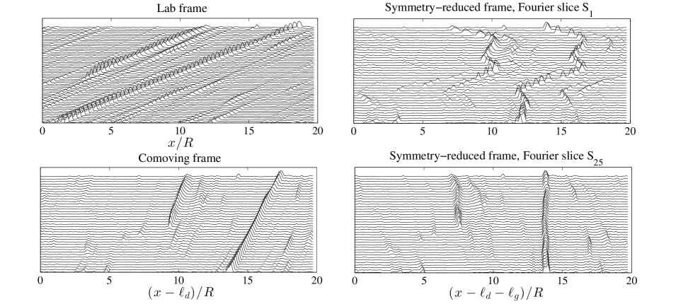
Figure 4.2: Symmetry reduction of LIF measurements: concentration profiles at increasing instants of time of the measured concentration $c(x,y=0,t)$ at the pipe centerline in the (top-left panel) fixed frame, (bottom-left panel) comoving frame $\left(x-\ell_{d},t\right)$, (right panels) symmetry-reduced frame $\left(x-\ell_{d}-\ell_{g},t\right)$ using Fourier slices (top) $S_{1}$ and (bottom) $S_{25}$. In each plot time increases from bottom to top. Associated 2-D patterns are shown in Fig. (4.1).

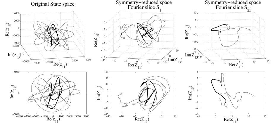
Figure 4.3: Symmetry reduction of LIF measurements: (left panels) Orbit trajectory $\mathbf{z}$ in the subspace $\left\{\mbox{Re}(z_{11}),\mbox{Im}(z_{13}),\mbox{Re}(z_{15})\right\}$ of the state space $\mathcal{P}$ associated with the passive scalar dynamics in the lab frame of Fig. (4.2) (see also Fig. (4.1)); (center panels) corresponding symmetry-reduced orbits $\mathbf{Z}$ in the subspace $\left\{\mbox{Re}(Z_{11}),\mbox{Im}(Z_{13}),\mbox{Re}(Z_{15})\right\}$ of the base manifold $\mathcal{M}$ associated with Fourier slices (center panels) $S_{1}$ and (right panels) $S_{25}$. The bold line indicates the excursion of the orbit while the concentration $c$ lingers above the threshold $0.95c_{\mathrm{max}}$ ($\Circle$ =initial time, $\times$=final time).

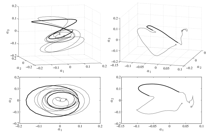
Figure 4.4: Symmetry reduction of LIF measurements: (left) Orbit trajectories $\mathbf{z}$ associated with the passive scalar dynamics in the lab frame (see panel (a) of Fig. (4.1)) projected onto the subspace ($a_{1},a_{2},a_{3}$) of the most energetic POD modes (right) corresponding desymmetrized orbit $\mathbf{Z}$ in the symmetry-reduced frame associated with the Fourier slice $S_{25}$. The bold line indicates the excursion of the orbit while the concentration $c$ lingers above the threshold $0.95c_{\mathrm{max}}$ ($\Circle$ =initial time, $\times$=final time).

4.2 Symmetry reduction of LIF measurements

In the section, we present a symmetry reduction of the acquired LIF measurements of turbulent pipe flows (see section 2.1). In particular, we study their evolution in physical space and in the associated state space $\mathcal{P}$ of dimension $N=40430$ equal to the total number of data image pixels ($65\times 622$).

As regards the choice of the Fourier slice $S_{j}$ it is in general entirely arbitrary. There is no unique way to quotient out the symmetry. The most likely choice would be $S_{1}$, but for our measurements this choice will not produce a physically meaningful symmetry reduction. Higher order slices are required.

In particular, Figs. (4.1) and (4.2) illustrate the space-time evolution of a passive scalar structure and concentration profiles. The top-left panel of Fig. (4.1) shows the dye concentration $c(x,t)$ at the pipe centerline in the fixed frame $(x,t)$ [see also Fig. (4.2)]. A drift in the streamwise direction $x$ is observed. The corresponding orbit $\mathbf{z}(t)$ in the subspace $\left\{\mbox{Re}(z_{11}),\mbox{Im}(z_{13}),\mbox{Re}(z_{15})\right\}$ of $\mathcal{P}$ is shown in the left panels of Fig. (4.3). Note that the excursion of the orbit while the concentration $c$ lingers above the threshold $0.95c_{\mathrm{max}}$ is complicated (bold line) since it wanders around its group orbit as a result of the drift induced by the translation symmetry. The bottom-left panel of Fig. (4.1) shows the space-time evolution in the comoving frame $\left(x-\ell_{d},t\right)$. Note that the dye concentration still experiences a significant drift (see also Fig. (4.2)). As a result, the associated orbit in state space still wanders around the group orbit. A proper choice of the Fourier slice can provide a physically meaningful symmetry-reduced frame. For example, if we choose the first Fourier mode slice $S_{1}$, the top-left panel of Fig. (4.1) depicts the associated evolution in the symmetry-reduced frame $\left(x-\ell_{d}-\ell_{g},t\right)$. Clearly, the symmetry is quotient out, but in the Fourier slice $S_{1}$ we observe a distorted shape-changing dynamics of the dye concentration. Instead, if we choose the Fourier slice $S_{25}$ the drift almost disappears in the corresponding symmetry-reduced frame, as shown in the bottom-left panel of Figure (4.1) [see also Fig. (4.2)]. Here, this slice is sufficient to symmetry-reduce the orbit $\mathbf{z}$ over the analyzed time span as its Fourier components $z_{k},$ with $k\sim 20-30$, never lingers near zero, whereas smaller or larger wavenumber modes can be small. The corresponding symmetry-reduced orbits $\mathbf{Z}(t)$ associated with $S_{1}$ and $S_{25}$ are computed from Eq. (4.4). Their time evolutions within the subspace $\left\{\mbox{Re}(Z_{11}),\mbox{Im}(Z_{13}),\mbox{Re}(Z_{15})\right\}$ of $\mathcal{M}$ are shown in the center and left panels of Fig. (4.3) respectively. Here, the excursion of the orbits while the concentration $c$ is high ($>0.95c_{\mathrm{max}}$) is marked as a bold line. Similar dynamics is also observed projecting the orbits onto the subspace of their respective most energetic proper orthogonal decomposition (POD) modes, as shown in Fig. (4.4). The POD projection of the symmetry-reduced orbit $\mathbf{Z}$ is performed within the corresponding symmetry-reduced space. Note that any two POD mode amplitudes are statistically uncorrelated by construction as any two components $Z_{p}$ and $Z_{q}$ chosen at random. Clearly, this does not imply that they are stochastically independent since they evolve on the quotient manifold $\mathcal{M}$, which is unknown. As an example, consider two random variables $X$ and $Y$ that satisfy $X^{2}+Y^{2}-1=0$. They are uncorrelated but not independent and POD projections will not help revealing the intrinsic manifold structure. Local linear embedding techniques may be more appropriate and appealing (Roweis & Saul (2000)), but they are beyond the scope of our work.

The top panels $a,c$ of Figure (4.5) show that geometric drifts associated with Fourier slices $S_{1}$ and $S_{25}$ are different and so the respective geometric phase velocities (see bottom panels $b,d$ of the same figure). Clearly, the dynamical component $U_{d}$ is the same since it does not depend on the symmetry-reduction scheme or slice. Note that $\ell_{g}$ is not the drift seen by an observer in the symmetry-reduced frame. If it were, the geometric phase velocity associated with the slice $S_{25}$ would be zero since the desymmetrized dye concentration field does not drift. If the same observer drifts by $\ell_{g}$ he will observe the dynamics in the comoving frame. This explains why the geometric phase velocity $U_{g}$ associated with the slice $S_{1}$ is negative between the time span $0.5<t/T_{d}<1$. With reference to Fig. (4.2), in that time interval an observer in the symmetry-reduced frame needs to decelerate in order to follow the dye concentration evolution seen in the comoving frame.

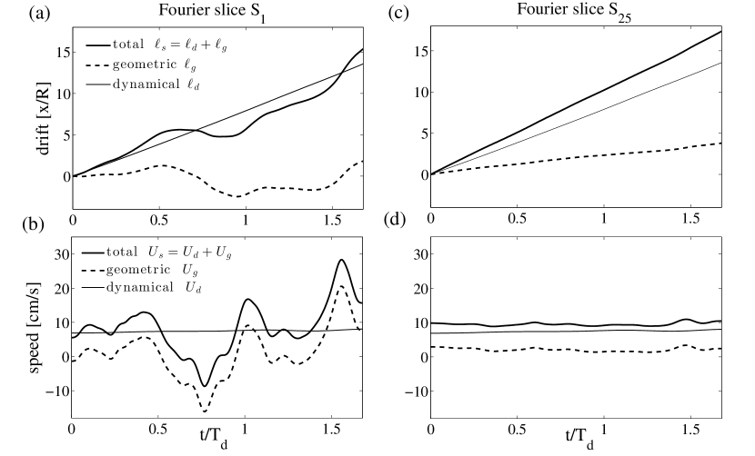
Figure 4.5: Symmetry reduction of LIF data using Fourier slice $S_{1}$ (panels a-b) and $S_{25}$ (panels $c,d$); (top panels $a,c$) total, dynamical and geometric drifts and (bottom panels $b,d$) corresponding velocities $U_{s}$, $U_{d}$ and $U_{g}$ associated with the orbit in state space of Fig. (4.3).

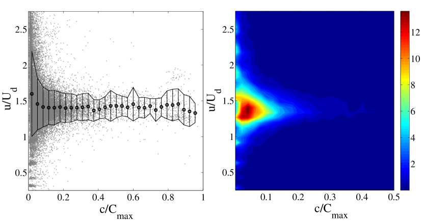
Figure 4.6: LIF experiments: (left) observed normalized dye concentration peak speed $u/U_{d}$ as a function of the amplitude peak $c/C_{\mathrm{max}}$, and (right) associated probability density function, with $C_{\mathrm{max}}$ denoting the observed maximum value of dye concentration over the whole data set.

The observed speed $u$ of dye concentration peaks is approximately 40% larger than the comoving frame velocity $U_{d}$, which changes slightly during the event. The excess speed $\delta u=u-U_{d}$ is fairly explained by the geometric phase velocity $U_{g}\approx 0.4U_{d}$ associated with slice $S_{25}$, as seen in panel $d$ of Figure (4.5). This appears to be a general trend of the flow as can be seen in Fig. (4.6), which shows the observed normalized speed $u/U_{d}$ of dye concentration peaks tracked in space as a function of their amplitude $c/C_{\mathrm{max}}$, and the associated probability density function, where $C_{\mathrm{max}}$ denotes the observed maximum value of dye concentration over the whole data set. As the peak amplitude increases, their speed $u$ tends to $1.43U_{d}$. Furthermore, in the symmetry-reduced frame, we observe the shape-changing dynamics of passive scalar structures (see bottom panel of Figure (4.2)). This induces the ’self-propulsion velocity’ $U_{g}$ of the flow structures similar to that of the motion of a swimmer at low Reynolds numbers (Shapere & Wilczek (1989)). Only when the geometric $U_{g}\ll U_{d}$, Taylor’s approximation is valid and, as a result the flow structures slightly deform as they are advected at the comoving frame or dynamical phase velocity $U_{d}$, which is close to the mean flow $U_{m}$.

5 Conclusions

We have presented a Fourier-based symmetry reduction scheme for dynamical systems with continuous translation symmetries. As an application, we have symmetry-reduced LIF measurements of fluorescent dye concentration fields tracing a turbulent pipe flow at Reynolds number $\mathsf{Re}=3200$. The symmetry reduction of LIF data on higher order Fourier slices revealed that the motion of passive scalar structures is associated with the dynamical and geometric phases of the corresponding orbits in state space. In particular, the observed speed $u\approx 1.43U_{d}$ of dye concentration peaks exceeds the comoving or convective velocity $U_{d}$. A physically meaningful representation of the quotient space by a proper choice of the Fourier slice explains the excess speed $\delta u=u-U_{d}$ as the geometric phase velocity $U_{g}\approx 0.43U_{d}$ associated with the Fourier slice $S_{25}$. Similar to the motion of a swimmer at low Reynolds number, the excess speed $\delta u$ is a ’self-propulsion’ velocity $U_{g}$ induced by the shape-changing dynamics of passive scalar structures as revealed in the symmetry-reduced frame.

Symmetry reduction is promising for the analysis of three-dimensional LIF and PIV measurements as well as simulated flows of pipe turbulence, in order to unveil the “shape of turbulence” and the hidden skeleton of its chaotic dynamics in state space. Further, the dependence of geometric phase velocities on the Reynolds number may shed some light on the nature of transition to turbulence, since the geometric phase is a measure of the curvature of the quotient manifold.

6 Acknowledgments

FF acknowledges the Georgia Tech graduate courses “Classical Mechanics II” taught by Jean Bellissard in Spring 2013 and “Nonlinear dynamics: Chaos, and what to do about it¿‘ taught by Predrag Cvitanović in Spring 2012. FF also thanks Alfred Shapere for discussions on geometric phases, and Federico Bonetto, Nazmi Burak Budanur, Bruno Eckhardt, Mohammad Farazmand, Chongchun Zeng as well as Evangelos Siminos for discussions on symmetry reduction.

7 Appendix

The time derivative of $\mathbf{z}=g_{\ell_{s}}(\mathbf{Z})$ is

$$\frac{\mathrm{d}\mathbf{z}}{\mathrm{d}t}=g_{\ell_{s}}\left(\frac{\mathrm{d}\mathbf{Z}}{\mathrm{d}t}\right)+\frac{\mathrm{d}\ell_{s}}{\mathrm{d}t}(\partial_{\ell_{s}}g)\mathbf{Z},$$

and the governing equation (4.2) for $\mathbf{z}$ yields

$$g_{\ell_{s}}\left(\frac{\mathrm{d}\mathbf{Z}}{\mathrm{d}t}\right)+\frac{\mathrm{d}\ell_{s}}{\mathrm{d}t}(\partial_{\ell_{s}}g)\mathbf{Z}-\mathcal{N_{\mathrm{1}}}(g_{\ell_{s}}\mathbf{Z})=0,$$

where the dependence of $\mathcal{N_{\mathrm{1}}}$ on $c_{0}$ and $\mathbf{\hat{\mathbf{\mathrm{\mathbf{v}}}}}$ is dropped for clarity of notation. Factoring out $g_{\ell_{s}}$ yields

$$g_{\ell_{s}}\left(\underset{T(\mathbf{Z})}{\frac{\mathrm{d}\ell}{\mathrm{d}t}\underbrace{g_{\ell_{s}}^{-1}(\partial_{\ell_{s}}g)\mathbf{Z}}}+\frac{\mathrm{d}\mathbf{Z}}{\mathrm{d}t}-\underset{\mathcal{N_{\mathrm{1}}}(\mathbf{Z})}{\underbrace{g_{\ell_{s}}^{-1}\mathcal{N_{\mathrm{1}}}(g_{\ell_{s}}\mathbf{Z})}}\right)=0.$$

This can be further simplified using (4.12) and noting that $\mathcal{N_{\mathrm{1}}}$ is invariant under translation symmetry, that is

$$g_{\ell_{s}}\left(\frac{\mathrm{d}\mathbf{Z}}{\mathrm{d}t}+\frac{\mathrm{d}\ell_{s}}{\mathrm{d}t}T(\mathbf{Z})-\mathcal{N_{\mathrm{1}}}(\mathbf{Z})\right)=0.$$

For translation symmetries, $g_{\ell_{s}}(q)=0$ if and only if $q=0$, thus the evolution of $\mathbf{Z}$ is governed by

$$\frac{\mathrm{d}\mathbf{Z}}{\mathrm{d}t}+\frac{\mathrm{d}\ell_{s}}{\mathrm{d}t}T(\mathbf{Z})-\mathcal{N_{\mathrm{1}}}(\mathbf{Z})=0.$$

References

- Banner et al. (2014) Banner, M. L., Barthelemy, X., Fedele, F., Allis, M., Benetazzo, A., Dias, F. & Peirson, W. L. 2014 Linking reduced breaking crest speeds to unsteady nonlinear water wave group behavior. Phys. Rev. Lett. 112, 114502.
- Berry (1984) Berry, M. V. 1984 Quantal phase factors accompanying adiabatic changes. Proceedings of the Royal Society of London. A. Mathematical and Physical Sciences 392 (1802), 45–57.
- Budanur et al. (2015) Budanur, N. B., Cvitanović, P., Davidchack, R. L. & Siminos, E. 2015 Reduction of so(2) symmetry for spatially extended dynamical systems. Phys. Rev. Lett. 114, 084102.
- Chandler & Kerswell (2013) Chandler, G. J. & Kerswell, R. R. 2013 Invariant recurrent solutions embedded in a turbulent two-dimensional kolmogorov flow. Journal of Fluid Mechanics 722, 554–595.
- Cvitanović (2013) Cvitanović, P. 2013 Recurrent flows: the clockwork behind turbulence. Journal of Fluid Mechanics 726, 1–4.
- Cvitanović et al. (2013) Cvitanović, P., Artuso, R., Mainieri, R., Tanner, G. & Vattay, G. 2013 Chaos: Classical and quantum.
- Cvitanović & Eckhardt (1991) Cvitanović, P. & Eckhardt, B. 1991 Periodic orbit expansions for classical smooth flows. Journal of Physics A: Mathematical and General 24 (5), L237.
- Cvitanović et al. (2012) Cvitanović, P. P., Borrero-Echeverry, D., Carroll, K. M., Robbins, B. & Siminos, E. 2012 Cartography of high-dimensional flows: a visual guide to sections and slices. Chaos 22, 047506.
- Del Álamo & Jimenez (2009) Del Álamo, J. C. & Jimenez, J. 2009 Estimation of turbulent convection velocities and corrections to taylor’s approximation. Journal of Fluid Mechanics 640, 5–26.
- Faisst & Eckhardt (2003) Faisst, H. & Eckhardt, B. 2003 Traveling waves in pipe flow. Phys. Rev. Lett. 91 (22), 224502.
- Fedele (2014a) Fedele, F. 2014a Geometric phases of water waves. Europhysics Letters 107 (69001).
- Fedele (2014b) Fedele, Francesco 2014b On certain properties of the compact zakharov equation. Journal of Fluid Mechanics 748, 692–711.
- Froehlich & Cvitanović (2012) Froehlich, S. & Cvitanović, P. 2012 Reduction of continuous symmetries of chaotic flows by the method of slices. Communications in Nonlinear Science and Numerical Simulation 17 (5), 2074 – 2084.
- Gibson et al. (2008) Gibson, J. F., Halcrow, J. & Cvitanović, P. 2008 Visualizing the geometry of state space in plane couette flow. Journal of Fluid Mechanics 611, 107–130.
- Gritsun (2011) Gritsun, A. 2011 Connection of periodic orbits and variability patterns of circulation for the barotropic model of atmospheric dynamics. Doklady Earth Sciences 438 (1), 636–640.
- Gritsun (2013) Gritsun, A. 2013 Statistical characteristics, circulation regimes and unstable periodic orbits of a barotropic atmospheric model. Philosophical Transactions of the Royal Society A: Mathematical, Physical and Engineering Sciences 371 (1991).
- Hannay (1985) Hannay, J H 1985 Angle variable holonomy in adiabatic excursion of an integrable hamiltonian. Journal of Physics A: Mathematical and General 18 (2), 221.
- Hopf (1931) Hopf, Heinz 1931 Über die abbildungen der dreidimensionalen sphäre auf die kugelfläche. Mathematische Annalen 104 (1), 637–665.
- Husemöller (1994) Husemöller, Dale 1994 Fibre Bundles, 3rd edn. Graduate Texts in Mathematics, Book 20 1. New York, Springer.
- Kreilos et al. (2014) Kreilos, T., Zammert, S. & Eckhardt, B. 2014 Comoving frames and symmetry-related motions in parallel shear flows. Journal of Fluid Mechanics 751, 685–697.
- Krogstad et al. (1998) Krogstad, P.-Å., Kaspersen, J. H. & Rimestad, S. 1998 Convection velocities in a turbulent boundary layer. Physics of Fluids 10 (4), 949–957.
- Pancharatnam (1956) Pancharatnam, S. 1956 Generalized theory of interference, and its applications. Proceedings of the Indian Academy of Sciences - Section A 44 (5), 247–262.
- Roweis & Saul (2000) Roweis, S. T. & Saul, L. K. 2000 Nonlinear dimensionality reduction by locally linear embedding. Science 290 (5500), 2323–2326.
- Rowley et al. (2003) Rowley, C. W., Kevrekidis, I. G., Marsden, J. E. & K., Lust 2003 Reduction and reconstruction for self-similar dynamical systems. Nonlinearity 16 (4), 1257.
- Rowley & Marsden (2000) Rowley, Clarence W. & Marsden, Jerrold E. 2000 Reconstruction equations and the karhunen–loève expansion for systems with symmetry. Physica D: Nonlinear Phenomena 142 (1–2), 1 – 19.
- Samuel & Bhandari (1988) Samuel, Joseph & Bhandari, Rajendra 1988 General setting for berry’s phase. Phys. Rev. Lett. 60, 2339–2342.
- Shapere & Wilczek (1989) Shapere, Alfred & Wilczek, Frank 1989 Geometry of self-propulsion at low reynolds number. Journal of Fluid Mechanics 198, 557–585.
- Siminos & Cvitanović (2011) Siminos, E. & Cvitanović, P. 2011 Continuous symmetry reduction and return maps for high-dimensional flows. Physica D: Nonlinear Phenomena 240 (2), 187 – 198.
- Simon (1983) Simon, Barry 1983 Holonomy, the quantum adiabatic theorem, and berry’s phase. Phys. Rev. Lett. 51 (24), 2167–2170.
- Steenrod (1999) Steenrod, Norman 1999 The Topology of Fibre Bundles. Princeton, University Press.
- Taylor (1938) Taylor, G. I. 1938 The spectrum of turbulence. Proceedings of the Royal Society of London. Series A - Mathematical and Physical Sciences 164 (919), 476–490.
- Tian & Roberts (2003) Tian, X. & Roberts, P. J.W. 2003 A 3d lif system for turbulent buoyant jet flows. Experiments in Fluids 35 (6), 636–647.
- Viswanath (2007) Viswanath, D. 2007 Recurrent motions within plane couette turbulence. Journal of Fluid Mechanics 580, 339–358.
- Wedin & Kerswell (2004) Wedin, H. & Kerswell, R. R. 2004 Exact coherent structures in pipe flow: travelling wave solutions. Journal of Fluid Mechanics 508, 333–371.
- Willis et al. (2013) Willis, A. P., Cvitanović, P. & Avila, M. 2013 Revealing the state space of turbulent pipe flow by symmetry reduction. Journal of Fluid Mechanics 721, 514–540.