A New Method for Indirect Mass Measurements using the Integral Charge Asymmetry at the LHC

Abstract

Processes producing a charged final state at the LHC have a positive or null integral charge asymmetry. We propose a novel method for an indirect measurement of the mass of these final states based upon the process integral charge asymmetry. We present this method in three stages. Firstly, the theoretical prediction of the integral charge asymmetry and its related uncertainties are studied through parton level cross sections calculations. Secondly, the experimental extraction of the integral charge asymmetry of a given signal, in the presence of some background, is performed using particle level simulations. Process dependent templates enable to convert the measured integral charge asymmetry into an estimated mass of the charged final state. Thirdly, a combination of the experimental and the theoretical uncertainties determines the full uncertainty of the indirect mass measurement.

This new method applies to all charged current processes at the LHC. In this article, we demonstrate its effectiveness at extracting the mass of the W boson, as a first step, and the sum of the masses of a chargino and a neutralino in case these supersymmetric particles are produced by pair, as a second step.

1 Introduction

Contrarily to most of the previous high energy particle colliders, the LHC is a charge asymmetric machine. For charged final states , denoted $FS^{\pm}$, the integral charge asymmetry, denoted $A_{C}$, is defined by

$$A_{C}=\frac{N(FS^{+})-N(FS^{-})}{N(FS^{+})+N(FS^{-})}$$ (1)

where $N(FS^{+})$ and $N(FS^{-})$ represent respectively the number of events bearing a positive and a negative charge in the FS.

For a $FS^{\pm}$ produced at the LHC in $p+p$ collisions, this quantity is positive or null, whilst it is always compatible with zero for a $FS^{\pm}$ produced at the TEVATRON in $p+\bar{p}$ collisions.

To illustrate the $A_{C}$ observable, let’s consider the Drell-Yan production of $W^{\pm}$ bosons in $p+p$ collisions. It is obvious for this simple $2\to 2$ s-channel process that more $W^{+}$ than $W^{-}$ are produced. Indeed, denoting $y_{W}$ the rapidity of the W boson, the corresponding range of the Björken x’s: $x_{1,2}=\frac{M_{W^{\pm}}}{\sqrt{s}}\times e^{\pm y_{W}}$, probes the charge asymmetric valence parton densities within the proton. This results in having more $U+\bar{D}\to W^{+}$ than $\bar{U}+D\to W^{-}$ configurations in the initial state (IS). Here U and D collectively and respectively represent the up and the down quarks.

In the latter case the dominant contribution to $A_{C}$ comes from the difference in rate between the $u+\bar{d}$ and the $d+\bar{u}$ quark currents in the IS. Using the usual notation $f(x,Q^{2})$ for the parton density functions (PDF) and within the leading order (LO) approximation, this can be expressed as:

$$A_{C}\approx\frac{u(x_{1,2},M_{W}^{2})\bar{d}(x_{2,1},M_{W}^{2})-\bar{u}(x_{1,2},M_{W}^{2})d(x_{2,1},M_{W}^{2})}{u(x_{1,2},M_{W}^{2})\bar{d}(x_{2,1},M_{W}^{2})+\bar{u}(x_{1,2},M_{W}^{2})d(x_{2,1},M_{W}^{2})}$$ (2)

where the squared four-momentum transfer $Q^{2}$ is set to $M_{W}^{2}$.

From equation 2, we can see that the $Q^{2}$ evolution of the parton density functions (PDFs) governs the $Q^{2}$ evolution of $A_{C}$. The former are known, up-to the NNLO in QCD, as solutions of the DGLAP equations Cafarella:2005zj . One could therefore think of using an analytical functional form to relate $A_{C}$ to the squared mass of the s-channel propagator, here $M_{W}^{2}$. However there are additional contributions to the $W^{\pm}$ inclusive production. At the Born level, some come from other flavour combinations in the IS of the s-channel, and some come from the u-channel and the t-channel. On top of this, there are higher order corrections. These extra contributions render the analytical expression of the $Q^{2}$ dependence of $A_{C}$ much more complicated. Therefore we choose to build process-dependent numerical mass template curves for $A_{C}$ by varying M${}_{FS^{\pm}}$. These mass templates constitute inclusive and flexible tools into which all the above-mentioned contributions to $A_{C}$ can be incorporated, they can very easily be built within restricted domain of the signal phase space imposed by kinematic cuts.

The $A_{C}$ for the $W^{\pm}\to\ell^{\pm}\nu$ production at the LHC is large enough to be measured and it has relatively small systematic uncertainties since it’s a ratio of cross sections. The differential charge asymmetry of this process in $p+p$ collisions have indeed been measured by the ATLAS Aad:2011yna , the CMS Chatrchyan:2012xt Chatrchyan:2013mza and the LHCb LHCb:2011xha experiments ATLAS:2011pha for the first times in their 2011 datasets.

In this article we exploit the $A_{C}$ to set a new type of constraint on the mass of the charged $FS^{\pm}$ as initially proposed in Djouadi:1998di Muanza:1st-note .

We’ll separate the study into two parts. The first one, in section 2, is dedicated to present in full length the method of indirect mass measurement that we propose on a known Standard Model (SM) process. We choose the $W^{\pm}\to\ell^{\pm}+\hbox to0.0pt{\kern 2.5pt/\hss}E_{T}$ inclusive production at the LHC to serve as a test bench.

In the second part, in section 3, we shall repeat the method on a "Beyond the Standard Model" (BSM) process. We choose a SUSY search process of high interest, namely

$$\tilde{\chi}^{\pm}_{1}+\tilde{\chi}^{0}_{2}\to 3\ell^{\pm}+\hbox to0.0pt{\kern 2.5pt/\hss}E_{T}.$$ (3)

For both the SM and the BSM processes, we obviously tag the sign of the FS by choosing a decay into one (or three) charged lepton(s) for which the sign is experimentally easily accessible.

It’s obvious that for these two physics cases other mass reconstruction methods exist. These standard mass reconstruction techniques are all based on the kinematics of the FS. For the $W^{\pm}\to\ell^{\pm}+\hbox to0.0pt{\kern 2.5pt/\hss}E_{T}$ process mass templates based upon the transverse mass allow to extract $M_{W^{\pm}}$ with an excellent precision that the new technique proposed here cannot match. In constrast, for the $\tilde{\chi}^{\pm}_{1}+\tilde{\chi}^{0}_{2}\to 3\ell^{\pm}+\hbox to0.0pt{\kern 2.5pt/\hss}E_{T}$ process, even if astute extensions of the transverse mass enable to acurrately measure some mass differences, no standard techniques is able to measure accurately the mass of the charged FS: $M_{FS^{\pm}}=M_{\tilde{\chi}^{\pm}_{1}}+M_{\tilde{\chi}^{0}_{2}}$.

Therefore this new mass reconstruction technique should not be viewed as an alternative to the standard techniques but rather as an unmined complement to them. In a few cases, especially where many FS particles escape detection, this new technique can be more accurate than the standard ones. It also has the advantage of being almost model independent.

For each signal process we sub-divide the method into four steps that are described in four sub-sections. In the first sub-sections 2.1 and 3.1, we start by deriving the theoretical $A_{C}$ template curves at the parton level.

In the second sub-sections 2.2 and 3.2, we place ourselves in the situation of an experimental measurement of the $A_{C}$ of the signal in the presence of some background. For that we generate samples of Monte Carlo (MC) events that we reconstruct using a fast simulation of the response of the ATLAS detector. This enables to account for the bias of the signal $A_{C}$ induced by the event selection. In addition we can quantify the bias of $A_{C}$ due to the residual contribution of some background processes passing this event selection.

Then, in the third sub-sections 2.3 and 3.3, we convert the measured $A_{C}$ into an estimated $M_{FS}$ using fitted experimental $A_{C}$ template curves that account for all the experimental uncertainties.

In the fourth sub-sections 2.4 and 3.4, we combine the theoretical and the experimental uncertainties on the signal $A_{C}$ to derive the full uncertainty of the indirect mass measurement. The conclusions are presented in section 4 and the prospects in section 5.

Note that we’ll always express the integral charge asymmetry in $\%$ and the mass of the charged final state in $GeV$ throughout this article. The uncertainty on the integral charge asymmetry $\delta A_{C}$ will also be expressed in $\%$ but will always represent an absolute uncertainty as opposed to a relative uncertainty with respect to $A_{C}$.

2 Inclusive Production of $W^{\pm}\to\ell^{\pm}\nu$

2.1 Theoretical Prediction of $A_{C}(W^{\pm}\to\ell^{\pm}\nu)$

In this section we calculate separately the cross sections of the "signed processes", i.e. the cross sections of the positive and negative FS: $\sigma^{+}=\sigma(p+p\to W^{+}\to\ell^{+}\nu)$ and $\sigma^{-}=\sigma(p+p\to W^{-}\to\ell^{-}\bar{\nu})$. The process integral charge asymmetry therefore writes:

$$A_{C}=\frac{\sigma^{+}-\sigma^{-}}{\sigma^{+}+\sigma^{-}}$$ (4)

2.1.1 Sources of Theoretical Uncertainties on $A_{C}$

Since these cross sections integration are numerical rather than analytical, they each have an associated statistical uncertainty $\delta\sigma^{\pm}_{Stat}$ due to the finite sampling of the process phase space. Even though these are relatively small we explicitely include them and we calculate the resulting statistical uncertainty on the process integral charge asymmetry: $\delta(A_{C})_{Stat}$ for which we treat $\delta\sigma^{+}_{Stat}$ and $\delta\sigma^{-}_{Stat}$ as uncorrelated uncertainties. Hence:

$$\delta(A_{C})_{Stat}=\frac{2}{(\sigma^{+}+\sigma^{-})^{2}}\sqrt{(\sigma^{-}\cdot\delta\sigma^{+}_{Stat})^{2}+(\sigma^{+}\cdot\delta\sigma^{-}_{Stat})^{2}}$$ (5)

For each cross section calculation we choose the central Parton Density Function (PDF) from a PDF set (or just the single PDF when there’s no associated uncertainty set). Whenever we use a PDF set, it contains $2N_{PDF}$ uncertainty PDFs on top of the central PDF fit, the PDF uncertainty is calculated as proposed in Campbell:2006wx :

$$\begin{cases}\delta(A_{C})_{PDF}^{Up}=\sqrt{\sum_{i=1}^{N_{PDF}}(Max[A_{C}(i)^{up}-A_{C}(0),A_{C}(i)^{down}-A_{C}(0),0])^{2}}\\ \delta(A_{C})_{PDF}^{Down}=\sqrt{\sum_{i=1}^{N_{PDF}}(Max[A_{C}(0)-A_{C}(i)^{up},A_{C}(0)-A_{C}(i)^{down},0])^{2}}\end{cases}$$ (6)

where $A_{C}(0)$, $A_{C}(i)^{up}$, and $A_{C}(i)^{down}$ represent the integral charge asymmetries calculated with $\sigma_{0}$, $\sigma_{i}^{up}$, and $\sigma_{i}^{down}$, respectively. $\sigma_{0}$ represents the cross section calculated with the central PDF fit. $\sigma_{i}^{up}$ represent the $N_{PDF}$ upward uncertainty PDFs such that generally $\sigma_{i}^{up}>\sigma_{0}$, and $\sigma_{i}^{down}$ represent the $N_{PDF}$ downward uncertainty PDFs such that generally $\sigma_{i}^{down}<\sigma_{0}$.

We choose the QCD renormalization and factorization scales: $\mu_{R}=\mu_{F}=\mu_{0}$ to be equal, and we choose a process dependent dynamical option to adjust the value of $\mu_{0}$ to the actual kinematics event by event. The scale uncertainty is evaluated using the usual factors 1/2 and 2 to calculate variations with respect to the central value $\mu_{0}$:

$$\begin{cases}\delta(A_{C})_{Scale}^{Up}=A_{C}(\mu_{0}/2)-A_{C}(\mu_{0})\\ \delta(A_{C})_{Scale}^{Down}=A_{C}(2\mu_{0})-A_{C}(\mu_{0})\end{cases}$$ (7)

The total theoretical uncertainty is defined as the sum in quadrature of the 3 sources:

$$\begin{cases}\delta(A_{C})_{Total}^{Up}=\sqrt{[\delta(A_{C})_{PDF}^{Up}]^{2}+[\delta(A_{C})_{Scale}^{Up}]^{2}+[\delta(A_{C})_{Stat}]^{2}}\\ \delta(A_{C})_{Total}^{Down}=\sqrt{[\delta(A_{C})_{PDF}^{Down}]^{2}+[\delta(A_{C})_{Scale}^{Down}]^{2}+[\delta(A_{C})_{Stat}]^{2}}\end{cases}$$ (8)

2.1.2 Setup and Tools for the Computation of $A_{C}$

We calculate the $\sigma^{+}=\sigma(p+p\to W^{+}\to\ell^{+}\nu)$ and $\sigma^{-}=\sigma(p+p\to W^{-}\to\ell^{-}\bar{\nu})$ cross sections and their uncertainties at $\sqrt{s}=$7 TeV using MCFM v5.8 Campbell:1999ah Campbell:2000bg Campbell:2002tg . We include both the $W^{\pm}+0Lp$ and the $W^{\pm}+1Lp$ matrix elements (ME) in the calculation in order to have a better representation of the $W^{\pm}$ inclusive production (the notation "Lp" stands for "light parton", i.e. u/d/s quarks or gluons). We set the QCD scales as $\mu_{R}=\mu_{F}=\mu_{0}=\sqrt{M^{2}(W^{\pm})+p_{T}^{2}(W^{\pm})}$ and we run the calculation at the QCD leading order (LO) and next-to-leading order (NLO). For both the phase space pre-sampling and the actual cross section integration, we run 10 times 20,000 sweeps of VEGAS Lepage:1980dq . We impose the following parton level cuts: $M(\ell^{\pm}\nu)>10$  GeV, $|\eta(\ell^{\pm})|<2.4$ and $p_{T}(\ell^{\pm})>20$  GeV. We artificially vary the input mass of the $W^{\pm}$ boson and we repeat the computations for the 3 following couples of respective LO and NLO PDFs: MRST2007lomod Sherstnev:2007nd - MRST2004nlo Martin:2004ir , CTEQ6L1 Pumplin:2002vw - CTEQ6.6 Nadolsky:2008zw , and MSTW2008lo68cl - MSTW2008nlo68cl MSTW2008 which are interfaced to MCFM through LHAPDF v5.7.1 Whalley:2005nh . As the LO is sufficient to present the method in detail, we’ll restrict ourselves to LO MEs and LO PDFs throughout the article for the sake of simplicity. We shall however provide the theoretical $A_{C}$ mass templates up to the NLO for the W process. And we recommend to establish them using the best theoretical calculations available for any use in a real data analysis, including at the minimum the QCD NLO corrections.

The MRST2007lomod is chosen as the default PDF throughout this article. The two other LO PDFs serve for comparison of the central value and the uncertainty of $A_{C}$ with respect to MRST2007lomod. In that regard, MSTW2008lo68cl is especially useful to estimate the impact of the $\delta(A_{C})_{PDF}$.

2.1.3 Modeling of the Theoretical $A_{C}(W^{\pm}\to e^{\pm}\nu_{e})$ Template Curves

The theoretical MRST2007lomod and MRST2004nlo raw template curves are obtained by sampling $A_{C}^{Raw}$ at different values of $M_{W^{\pm}}$. The corresponding theoretical uncertainties are also calculated: $A_{C}^{Raw}\pm\delta A_{C}^{Raw}$. This discrete sampling is then transformed into a continuous template curve through a fit using a functional form $A_{C}^{Fit}=f(M_{W^{\pm}})$ which is constrained by the theoretical uncertainties.

We have considered three different types of functional forms for these fits with $f$ being either a:

1. polynomial of logarithms: $f(x)=\sum\limits_{i=0}^{N_{FP}}A_{i}\times\{Log(x)\}^{i}$

2. polynomial of logarithms of logarithms: $f(x)=\sum\limits_{i=0}^{N_{FP}}A_{i}\times\{Log[Log(x)]\}^{i}$

3. series of Laguerre polynomials: $f(x)=\sum\limits_{i=0}^{N_{FP}}A_{i}\times L_{n}(x)$ where $L_{n}(x)=\frac{e^{x}}{n!}\frac{d^{n}}{dx^{n}}(e^{-x}x^{n}).$

The types of functional forms that we’re considering are not arbitrary, they are all related to parametrizations of solutions of the DGLAP equations for the evolution of the PDFs. The polynomial of logarithms of logarithms is inspired by an expansion of the PDF in series of $Log[Log(Q^{2})]$ as suggested in Cafarella:2005zj . The polynomial of logarithms was just the simplest approximation of the aforementioned series that we first considered. And the expansion of the PDF in series of Laguerre polynomials is proposed in Schoeffel:1998tz .

In the Appendix A, we give a numerical example of the evolution of the $u(x,Q^{2})$, $\bar{u}(x,Q^{2})$, $d(x,Q^{2})$, $\bar{d}(x,Q^{2})$ proton density functions calculated with QCDNUM Botje:2010ay and the
MSTW2008nlo68cl PDF. We also provide a few toy models to justify the main properties of the functional forms used for $A_{C}^{Fit}$.

Ultimately, the model of the theoretical template curve uses the functional form $f$ for the $A_{C}^{Fit}$ central values and re-calculate their uncertainty $\delta A_{C}^{Fit}$ by accounting for the correlations between the uncertainties of the fit parameters:

$$(\delta A_{C}^{Fit})^{2}=(\delta f)^{2}=\sum\limits_{i=0}^{N_{FP}}\sum\limits_{j>i}^{N_{FP}}\left(\frac{\partial f}{\partial A_{i}}\right)^{2}\cdot VAR(A_{i})+2\cdot\frac{\partial f}{\partial A_{i}}\cdot\frac{\partial f}{\partial A_{j}}\cdot COVAR(A_{i},A_{j})$$ (9)

The diagonal and off-diagonal elements of the fit uncertainty matrix are denoted $VAR(A_{i})$ and $COVAR(A_{i},A_{j})$, they correspond to the usual variances of the parameters and the covariances amongst them, respectively.

The number of fit parameters $N_{FP}$ is taken as the minimum integer necessary to get a good $\chi^{2}/N_{dof}$ for the fit and it is adjustable for each $A_{C}$ template curve.

Comparing the three types of polynomials cited above as functional forms to fit all the $A_{C}$ template curves of sub-sections 2.1 and 3.1, we find that the polynomials of logarithms of logarithms of $Q$ give the best fits. They are henceforth chosen as the default functional form to model the $Q$ evolution of $A_{C}$ throughout this article.

2.1.4 $A_{C}(W^{\pm}\to e^{\pm}\nu_{e})$ Template Curves for MRST

$\rm M_{W^{\pm}}$	$A_{C}$	$\delta(A_{C})_{Stat}$	$\delta(A_{C})_{Scale}$	$\delta(A_{C})_{PDF}$	$\delta(A_{C})_{Total}$
( GeV)	($\%$)	($\%$)	($\%$)	($\%$)	($\%$)
20.1	LO: 2.20	$\pm 0.24$	${}^{+0.47}_{+0.10}$	0.00	${}^{+0.52}_{-0.26}$
	NLO: 2.09	$\pm 0.11$	${}^{+0.04}_{-0.14}$	0.00	${}^{+0.12}_{-0.18}$
40.2	LO: 6.77	$\pm$0.12	${}^{+0.02}_{-0.11}$	0.00	${}^{+0.12}_{-0.16}$
	NLO: 8.05	$\pm 0.07$	${}^{-0.18}_{-0.06}$	0.00	${}^{+0.19}_{-0.09}$
80.4	LO: 20.18	$\pm$0.06	${}^{+0.05}_{-0.03}$	0.00	${}^{+0.08}_{-0.07}$
	NLO: 21.49	$\pm 0.03$	${}^{-0.08}_{-0.00}$	0.00	${}^{+0.09}_{-0.03}$
160.8	LO: 29.39	$\pm$0.05	${}^{+0.00}_{+0.03}$	0.00	${}^{+0.05}_{-0.06}$
	NLO: 30.55	$\pm 0.03$	${}^{-0.02}_{-0.01}$	0.00	${}^{+0.04}_{-0.03}$
321.6	LO: 35.92	$\pm$0.05	${}^{-0.11}_{+0.10}$	0.00	${}^{+0.11}_{-0.11}$
	NLO: 36.90	$\pm 0.03$	${}^{-0.05}_{-0.04}$	0.00	${}^{+0.06}_{-0.05}$
643.2	LO: 43.99	$\pm$0.05	${}^{-0.14}_{+0.13}$	0.00	${}^{+0.15}_{-0.14}$
	NLO: 45.11	$\pm 0.03$	${}^{-0.05}_{-0.05}$	0.00	${}^{+0.06}_{-0.06}$
1286.4	LO: 52.36	$\pm$0.06	${}^{+0.03}_{-0.02}$	0.00	${}^{+0.07}_{-0.07}$
	NLO: 55.33	$\pm 0.04$	${}^{+0.01}_{-0.02}$	0.00	${}^{+0.04}_{-0.04}$

Table 1: The MRST $A_{C}$ table with the breakdown of the different sources of theoretical uncertainty. The MRST2007lomod PDF is used for the LO and the MRST2004nlo for the NLO.

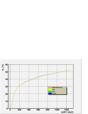
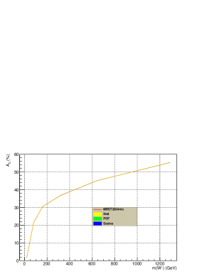
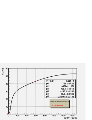
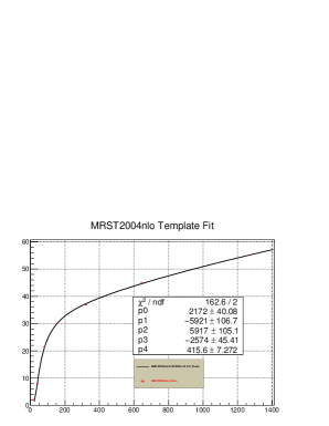
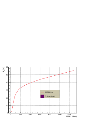
Figure 1: The theoretical MRST $A_{C}$ template curves at LO with MRST2007lomod on the left-hand side (LHS) and NLO with the MRST2004nlo on the right-hand side (RHS). The raw curve with its uncertainty bands, the corresponding fitted curve and the fitted curve with the correlations between the fit parameters uncertainties are displayed on the top, the middle and the bottom rows, respectively.

The theoretical MRST2007lomod and MRST2004nlo $A_{C}$ template curves are obtained from the signed cross sections used for table 1. Since there is no MRST2007lomod PDF uncertainty set, we simply set $\delta(A_{C})_{PDF}=0$. In this case, $\delta_{Total}^{Theory}A_{C}=\sqrt{\delta_{Stat}^{2}A_{C}+\delta_{Scale}^{2}A_{C}}$. Figure 1 displays the fit to the $A_{C}$ template curve using a polynomial of $Log\left(Log(Q)\right)$. In the case of the MRST2007lomod PDF, it is sufficient to limit the polynomial to the degree $N_{FP}=5$ to fit the $A_{C}$ template curve in the following (default) range: $M_{W^{\pm}}\in[15,1500]\rm\ GeV$.

$\rm M_{W^{\pm}}$	$A_{C}^{Fit}$	$\delta A^{Fit}_{C}$
( GeV)	($\%$)	($\%$)
20.1	LO: 1.35	$\pm 0.10$
	NLO: 2.00	$\pm 0.12$
40.2	LO: 7.27	$\pm 0.07$
	NLO: 8.31	$\pm 0.08$
80.4	LO: 19.93	$\pm 0.05$
	NLO: 21.12	$\pm 0.05$
160.8	LO: 29.46	$\pm 0.04$
	NLO: 30.49	$\pm 0.04$
321.6	LO: 36.29	$\pm 0.04$
	NLO: 37.29	$\pm 0.04$
643.2	LO: 43.07	$\pm 0.05$
	NLO: 44.61	$\pm 0.04$
1286.4	LO: 52.43	$\pm 0.06$
	NLO: 55.40	$\pm 0.04$

Table 2: The MRST $A_{C}^{Fit}$ table with $\delta A_{C}^{Fit}$ calculated using Eq. 9. The MRST2007lomod PDF is used at LO and the MRST2004nlo one is used at NLO.

2.1.5 $A_{C}(W^{\pm}\to e^{\pm}\nu_{e})$ Template Curves for CTEQ6

The theoretical CTEQ6L1 and CTEQ6.1 $A_{C}$ template curves are obtained from the signed cross sections used for table 3.

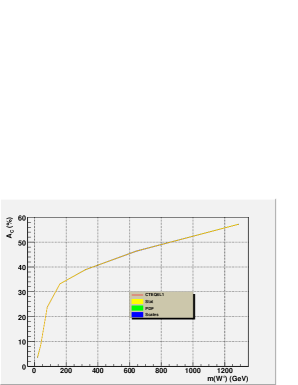
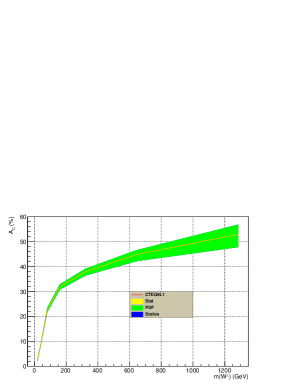
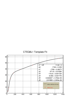
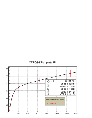
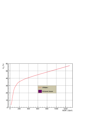
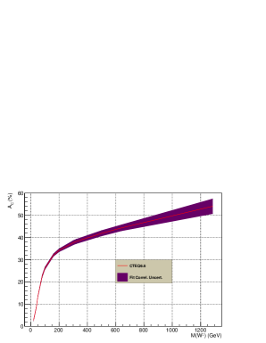
Figure 2: The theoretical CTEQ6 $A_{C}$ template curves at LO with CTEQ6L1 (LHS) and NLO with the CTEQ6.6 (RHS). The raw curve with its uncertainty bands, the corresponding fitted curve and the fitted curve with the correlations between the fit parameters uncertainties are displayed on the top, the middle and the bottom rows, respectively.

$\rm M_{W^{\pm}}$	$A_{C}$	$\delta(A_{C})_{Stat}$	$\delta(A_{C})_{Scale}$	$\delta(A_{C})_{PDF}$	$\delta(A_{C})_{Total}$
( GeV)	($\%$)	($\%$)	($\%$)	($\%$)	($\%$)
20.1	LO: 3.70	$\pm 0.24$	${}^{-0.27}_{+0.11}$	0.00	${}^{+0.36}_{-0.26}$
	NLO: 2.76	$\pm 0.11$	${}^{-0.24}_{-0.13}$	${}^{+0.37}_{-0.39}$	${}^{+0.45}_{-0.43}$
40.2	LO: 8.65	$\pm 0.12$	${}^{-0.02}_{-0.00}$	0.00	${}^{+0.12}_{-0.12}$
	NLO: 8.75	$\pm 0.07$	${}^{+0.09}_{-0.09}$	${}^{+0.38}_{-0.41}$	${}^{+0.40}_{-0.43}$
80.4	LO: 23.81	$\pm 0.06$	${}^{+0.07}_{-0.06}$	0.00	${}^{+0.09}_{-0.08}$
	NLO: 22.67	$\pm 0.03$	${}^{+0.14}_{-0.20}$	${}^{+0.74}_{-0.85}$	${}^{+0.75}_{-0.87}$
160.8	LO: 33.21	$\pm 0.05$	${}^{+0.01}_{-0.00}$	0.00	${}^{+0.05}_{-0.05}$
	NLO: 31.99	$\pm 0.02$	${}^{+0.23}_{-0.24}$	${}^{+0.86}_{-1.11}$	${}^{+0.89}_{-1.14}$
321.6	LO: 38.90	$\pm 0.05$	${}^{-0.09}_{+0.07}$	0.00	${}^{+0.10}_{-0.09}$
	NLO: 37.99	$\pm 0.03$	${}^{+0.18}_{-0.18}$	${}^{+1.11}_{-1.52}$	${}^{+1.12}_{-1.53}$
643.2	LO: 46.38	$\pm 0.05$	${}^{-0.14}_{0.13}$	0.00	${}^{+0.15}_{-0.14}$
	NLO: 44.83	$\pm 0.03$	${}^{+0.06}_{-0.09}$	${}^{+1.76}_{-2.64}$	${}^{+1.76}_{-2.64}$
1286.4	LO: 57.17	$\pm 0.06$	${}^{-0.06}_{+0.06}$	0.00	${}^{+0.08}_{-0.08}$
	NLO: 52.97	$\pm 0.04$	${}^{+0.05}_{+0.04}$	${}^{+3.90}_{-5.10}$	${}^{+3.90}_{-5.10}$

Table 3: The CTEQ6 $A_{C}$ table with the breakdown of the different sources of theoretical uncertainty. The CTEQ6L1 PDF is used at LO and the CTEQ6.6 one is used at NLO.

$\rm M_{W^{\pm}}$	$A_{C}^{Fit}$	$\delta A^{Fit}_{C}$
( GeV)	($\%$)	($\%$)
20.1	LO: 3.40	$\pm 0.09$
	NLO: 2.76	$\pm 0.44$
40.2	LO: 8.85	$\pm 0.06$
	NLO: 8.76	$\pm 0.42$
80.4	LO: 23.59	$\pm 0.04$
	NLO: 22.57	$\pm 0.64$
160.8	LO: 33.24	$\pm 0.04$
	NLO: 32.11	$\pm 0.66$
321.6	LO: 39.11	$\pm 0.04$
	NLO: 38.23	$\pm 1.08$
643.2	LO: 45.67	$\pm 0.05$
	NLO: 44.41	$\pm 1.43$
1286.4	LO: 57.24	$\pm 0.07$
	NLO: 54.11	$\pm 3.42$

Table 4: The CTEQ6 $A_{C}^{Fit}$ table with $\delta A_{C}^{Fit}$ calculated using Eq. 9. The CTEQ6L1 PDF is used at LO and the CTEQ6.6 one is used at NLO.

2.1.6 $A_{C}(W^{\pm}\to e^{\pm}\nu_{e})$ Template Curves for MSTW2008

The theoretical MSTW2008lo68cl and MSTW2008nlo68cl $A_{C}$ template curves are obtained from the signed cross sections used for table 5.

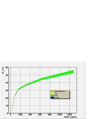
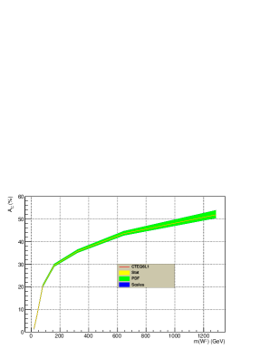
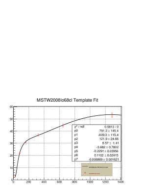
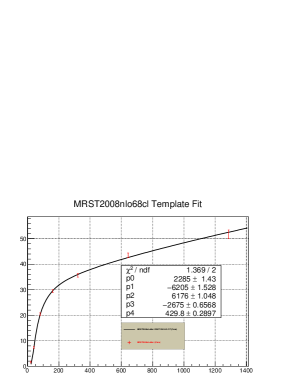
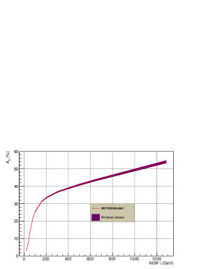
Figure 3: The theoretical MSTW2008 $A_{C}$ template curves at LO with MSTW2008lo68cl (LHS) and NLO with the MSTW2008nlo68cl (RHS). The raw curve with its uncertainty bands and the corresponding fitted curve are displayed on the LHS and on the RHS, respectively.

$\rm M_{W^{\pm}}$	$A_{C}$	$\delta(A_{C})_{Stat}$	$\delta(A_{C})_{Scale}$	$\delta(A_{C})_{PDF}$	$\delta(A_{C})_{Total}$
( GeV)	($\%$)	($\%$)	($\%$)	($\%$)	($\%$)
20.1	LO: 3.07	$\pm$0.24	${}^{-0.21}_{+0.14}$	${}^{+0.46}_{-0.40}$	${}^{+0.56}_{-0.49}$
	NLO: 1.64	$\pm 0.12$	${}^{-0.08}_{-0.17}$	${}^{+0.29}_{-0.31}$	${}^{+0.32}_{-0.37}$
40.2	LO: 7.85	$\pm$0.12	${}^{+0.10}_{+0.07}$	${}^{+0.43}_{-0.33}$	${}^{+0.46}_{-0.36}$
	NLO: 7.35	$\pm 0.07$	${}^{+0.05}_{-0.06}$	${}^{+0.30}_{-0.33}$	${}^{+0.31}_{-0.34}$
80.4	LO: 22.24	$\pm$0.06	${}^{+0.15}_{+0.13}$	${}^{+0.64}_{-0.42}$	${}^{+0.66}_{-0.44}$
	NLO: 20.47	$\pm 0.03$	${}^{-0.06}_{-0.01}$	${}^{+0.48}_{-0.46}$	${}^{+0.48}_{-0.46}$
160.8	LO: 31.19	$\pm$0.05	${}^{+0.21}_{+0.19}$	${}^{+0.78}_{-0.53}$	${}^{+0.81}_{-0.57}$
	NLO: 29.52	$\pm 0.03$	${}^{-0.10}_{+0.02}$	${}^{+0.62}_{-0.51}$	${}^{+0.63}_{-0.51}$
321.6	LO: 36.96	$\pm$0.05	${}^{+0.16}_{+0.33}$	${}^{+0.96}_{-0.70}$	${}^{+0.97}_{-0.77}$
	NLO: 35.73	$\pm 0.03$	${}^{-0.05}_{-0.05}$	${}^{+0.76}_{-0.59}$	${}^{+0.76}_{-0.59}$
643.2	LO: 44.63	$\pm$0.06	${}^{+0.17}_{+0.41}$	${}^{+1.28}_{-0.96}$	${}^{+1.29}_{-1.05}$
	NLO: 43.58	$\pm 0.03$	${}^{-0.08}_{-0.03}$	${}^{+1.05}_{-0.78}$	${}^{+1.05}_{-0.78}$
1286.4	LO: 53.66	$\pm$0.07	${}^{+0.31}_{+0.33}$	${}^{+2.39}_{-1.28}$	${}^{+2.42}_{-1.32}$
	NLO: 51.92	$\pm 0.04$	${}^{+0.03}_{+0.02}$	${}^{+1.99}_{-1.45}$	${}^{+1.99}_{-1.45}$

Table 5: The MSTW2008lo68cl $A_{C}$ table with the breakdown of the different sources of theoretical uncertainty. The MSTW2008lo68cl PDF is used at LO and the MSTW2008nlo68cl one is used at NLO.

In this case, the PDF uncertainty is provided and it turns out to be the dominant source of theoretical uncertainty on $A_{C}$.

$\rm M_{W^{\pm}}$	$A_{C}^{Fit}$	$\delta A^{Fit}_{C}$
( GeV)	($\%$)	($\%$)
20.1	LO: 3.05	$\pm 0.38$
	NLO: 1.63	$\pm 0.26$
40.2	LO: 7.90	$\pm 0.26$
	NLO: 7.39	$\pm 0.21$
80.4	LO: 21.89	$\pm 0.27$
	NLO: 20.30	$\pm 0.22$
160.8	LO: 31.35	$\pm 0.31$
	NLO: 29.59	$\pm 0.26$
321.6	LO: 37.22	$\pm 0.40$
	NLO: 35.99	$\pm 0.34$
643.2	LO: 43.49	$\pm 0.57$
	NLO: 42.61	$\pm 0.51$
1286.4	LO: 54.08	$\pm 0.83$
	NLO: 52.53	$\pm 0.74$

Table 6: The MSTW2008lo68cl $A_{C}^{Fit}$ table with $\delta A_{C}^{Fit}$ calculated using equation 9. The MSTW2008lo68cl PDF is used at LO and the MSTW2008nlo68cl one is used at NLO.

2.1.7 Comparing the Different $A_{C}$ Template Curves

At this stage, it’s interesting to compare the $A_{C}$ template curves produced with different PDFs using MCFM. From figure 4 we can see that the $A_{C}$ of the different PDF used at LO and at NLO are in agreement at the $\pm 2\sigma$ level, provided that we switch the reference to a PDF set containing uncertainty PDFs. This figure also displays the $\frac{A_{C}^{NLO}}{A_{C}^{LO}}$ ratios for the three families of PDFs used. These ratios are almost flat with respect to $M_{W^{\pm}}$ over the largest part of our range of interest. However at the low mass ends they vary rapidly. As we illustrate in the Appendix A, these integral charge asymmetry ratios can be fitted by the same functional forms as the $A_{C}^{LO}$ and $A_{C}^{NLO}$.

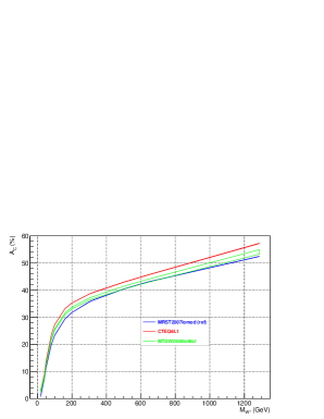
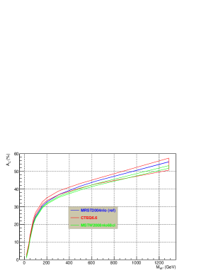
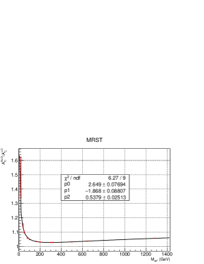
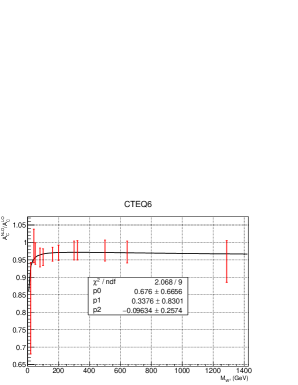
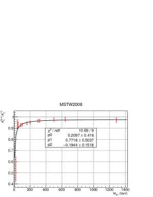
Figure 4: Comparison between the $A_{C}$ template curves. The top LHS plot compares the LO PDFs: MRST2007lomod (blue, ref. curve), CTEQ6L1 (red), MSTW2008lo68cl (green). The top RHS plot compares the NLO PDFs: MRST2004nlo (blue, ref. curve), CTEQ6.6 (red), MSTW2008nlo68cl (green). The middle and the bottom rows display the $\frac{A_{C}^{NLO}}{A_{C}^{LO}}$ fitted by the same functional forms as the $A_{C}^{LO}$ template curves.

2.2 Experimental Measurement of $A_{C}(W^{\pm}\to\ell^{\pm}\nu)$

The aim of this sub-section is to study the biases on $A_{C}$ due to two different sources: the event selection and the residual background remaining after the latter cuts are applied.

2.2.1 Monte Carlo Generation

To quantify these biases we generate Monte Carlo (MC) event samples using the following LO generator: Herwig++ v2.5.0 Gieseke:2011na . We adopt a tune of the underlying event derived by the ATLAS collaboration Aad:2011qe and we use accordingly the MRST2007lomod Sherstnev:2007nd PDF.

Herwig++ mainly uses $2\to 2$ LO ME that we denote in the standard way: $1+2\to 3+4$. For all the non-resonant processes, the production is splitted into bins of $M$, where $M=M(3,4)$ is the invariant mass of the two outgoing particles.

For the single vector boson ("V+jets") production, where V stands for $W^{\pm}$ and $\gamma^{*}/Z$, we mix in the same MC samples the contributions from the pure Drell-Yan process V+0Lp ME and the V+1Lp ME. For all the SM processes a common cut of $M>10\rm\ GeV$ is applied.

All the samples are normalized using the Herwig++ cross section multiplied by a K-factor that includes at least the NLO QCD corrections. We’ll denote NLO (respectively NNLO) K-factor the ratio: $\frac{\sigma_{NLO}}{\sigma_{LO}}$ (respectively $\frac{\sigma_{NNLO}}{\sigma_{LO}}$). We choose not the apply such higher order corrections to the normalization of the following non-resonant inclusive processes:

• light flavour QCD (denoted QCD LF): $2\to 2$ MEs involving $u/d/s/g$ partons

• heavy flavour QCD (denoted QCD HF): $c+\bar{c}$ and $b+\bar{b}$

• prompt photon productions: $\gamma+jets$ and $\gamma+\gamma$

Despite their large cross sections these non-resonant processes will turn out to have very low efficiencies and to represent a small fraction of the remaining background in the event selection used in the analyses we perform.

The NNLO K-factors for the $\gamma^{*}/Z(\to\ell^{\pm}\ell^{\mp})$ process are derived from PHOZR Hamberg:1990np with $\mu_{R}=\mu_{F}=M(\ell^{\pm}\ell^{\mp})$ and using the MSTW2008nnlo68cl PDF for $\sigma_{NNLO}$ and the MRST2007lomod one for $\sigma_{LO}$.

The top pairs and single top Campbell:2004ch Campbell:2009ss NLO K-factors are obtained by running MCFM v5.8 using the MSTW2008nlo68cl and the MSTW2008lo68cl PDFs for the numerator and the denominator respectively, with the QCD scales set as follows: $\mu_{R}=\mu_{F}=\hat{s}$.

2.2.2 Fast Simulation of the Detector Response

We use the following setup of Delphes v1.9 Ovyn:2009tx to get a fast simulation of the ATLAS detector response as well as a crude emulation of its trigger. The generated MC samples are written in the HepMC v2.04.02 format Dobbs:2001ck and passed through Delphes.

For the object reconstruction we also use Delphes defaults, with the exception of utilizing the "anti-kT" jet finder Cacciari:2008gp with a cone radius of $\Delta R=\sqrt{(\Delta\eta)^{2}+(\Delta\phi)^{2}}=0.4$.

2.2.3 Analyses of the $W^{\pm}\to\ell^{\pm}\nu$ Process

We consider only the electron and the muon channels. For these analyses we set the integrated luminosity to $\int{\cal L}dt=1\ fb^{-1}$.

Instead of trying to derive unreliable systematic uncertainties for these analyses using Delphes, we choose to use realistic values as quoted in actual LHC data analysis publications. We choose the analyses with the largest data samples so as to reduce as much as possible the statistical uncertainties in their measurements but also to benefit from the largest statistics for the data samples utilized to derive their systematic uncertainties. This choice leads us to quote systematic uncertainties from analyses performed by the CMS collaboration. Namely we use:

$$\delta_{Syst}A_{C}(W^{\pm}\to e^{\pm}\nu_{e})=1.0\%$$ (10)

$$\delta_{Syst}A_{C}(W^{\pm}\to\mu^{\pm}\nu_{\mu})=0.4\%$$ (11)

The values quoted in equations 10 and 11 come from references Chatrchyan:2012xt and Chatrchyan:2013mza , respectively.

And to get an estimate of the uncertainty on a ratio of number of expected events we use the systematics related to the measurement of the following cross sections ratio

$$\sigma(pp\to W^{\pm}\to\ell^{\pm}\nu_{\ell})/\sigma(pp\to\gamma^{*}/Z\to\ell^{\pm}\ell^{\mp})$$ (12)

which amounts to $1.0\%$ CMS:2011aa .

2.2.4. a. The Electron Channel

2.2.4. a.1. Event Selection in the Electron Channel

The following cuts are applied:

• $p_{T}(e^{\pm})>25\rm\ GeV$

• $|\eta(e^{\pm})|<1.37\rm\ or\ 1.53<|\eta(e^{\pm})|<2.4$

• Tracker Isolation: reject events with additional tracks of $p_{T}>2$ GeV within a cone of $\Delta R=0.5$ around the direction of the $e^{\pm}$ track

• Calorimeter Isolation: the ratio of, the scalar sum of $E_{T}$ deposits in the calorimeter within a cone of $\Delta R=0.5$ around the direction of the $e^{\pm}$, to the $p_{T}(e^{\pm})$, must be less than 1.2

• $\hbox to0.0pt{\kern 2.5pt/\hss}E_{T}>25\rm\ GeV$

• $M_{T}=\sqrt{2p_{T}(\ell^{\pm})\hbox to0.0pt{\kern 2.5pt/\hss}E_{T}[1-cos\Delta\phi(\ell^{\pm},\hbox to0.0pt{\kern 2.5pt/\hss}E_{T})]}>40\rm\ GeV$

• Reject events with an additional leading isolated muon: $\mu^{\pm}_{1}$

• Reject events with an additional trailing isolated electron: $e^{\pm}_{2}$

• Reject events with an additional second track ($Track_{2}$) such that:

  $$\begin{cases}Q(e^{\pm}_{1})=-Q(Track_{2})\\ 3<p_{T}(Track_{2})<10\rm\ GeV\\ M[e_{1}^{\pm},Track_{2}]>50\rm\ GeV\end{cases}$$

The corresponding selection efficiencies and event yields (expressed in thousanths of events) are reported in table 7. Figure 5 displays the $\hbox to0.0pt{\kern 2.5pt/\hss}E_{T}$ distribution after the event selection in the electron channel (LHS) and in the muon channel (RHS).

$Process$	$\epsilon$	$N_{exp}$	$A_{C}\pm\delta A_{C}^{Stat}$
	($\%$)	(k evts)	($\%$)
Signal: $W^{\pm}\to e^{\pm}\nu_{e}$
$M(W^{\pm})=40.2\rm\ GeV$	$0.81\pm 0.01$	290.367	$9.66\pm 1.57$
$M(W^{\pm})=60.3\rm\ GeV$	$13.69\pm 0.05$	2561.508	$11.22\pm 0.38$
$M(W^{\pm})=\underline{80.4}\rm\ GeV$	$29.59\pm 0.04$	3343.195	$16.70\pm 0.18$
$M(W^{\pm})=100.5\rm\ GeV$	$39.19\pm 0.07$	2926.093	$20.77\pm 0.22$
$M(W^{\pm})=120.6\rm\ GeV$	$44.84\pm 0.07$	2357.557	$23.19\pm 0.21$
$M(W^{\pm})=140.7\rm\ GeV$	$48.66\pm 0.07$	1899.820	$25.29\pm 0.20$
$M(W^{\pm})=160.8\rm\ GeV$	$51.28\pm 0.07$	1527.360	$26.87\pm 0.19$
$M(W^{\pm})=201.0\rm\ GeV$	$54.54\pm 0.07$	1.032	$29.06\pm 0.18$
Background	-	$91.614\pm 1.706$	$10.07\pm 0.15$
$W^{\pm}\to\mu^{\pm}\nu_{\mu}/\tau^{\pm}\nu_{\tau}/q\bar{q\prime}$	$0.211\pm 0.003$	$71.350$	$12.92\pm 1.25$
$t\bar{t}$	$5.76\pm 0.02$	6.600	$1.00\pm 0.37$
$t+b,\ t+q(+b)$	$3.59\pm 0.01$	1.926	$28.97\pm 0.35$
$W+W,\ W+\gamma^{*}/Z,\ \gamma^{*}/Z+\gamma^{*}/Z$	$2.94\pm 0.01$	2.331	$10.65\pm 0.35$
$\gamma+\gamma,\ \gamma+jets,\ \gamma+W^{\pm},\ \gamma+Z$	$0.201\pm 0.001$	0.759	$17.25\pm 0.53$
$\gamma^{*}/Z$	$0.535\pm 0.001$	5.746	$4.43\pm 0.23$
QCD HF	$(0.44\pm 0.17)\times 10^{-4}$	1.347	$14.29\pm 37.41$
QCD LF	$(0.87\pm 0.33)\times 10^{-4}$	1.555	$71.43\pm 26.45$

Table 7: Selection efficiencies, event yields and integral charge asymmetries for the $W^{\pm}\to e^{\pm}\nu_{e}$ analysis.

The non-resonant background processes represent just $\sim 4\%$ of the total background after the event selection, this justifies the approximation of not to include the NLO QCD corrections to their normalizations.

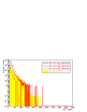
Figure 5: $\hbox to0.0pt{\kern 2.5pt/\hss}E_{T}$ distribution after the event selection is applied for the $W^{\pm}\to e^{\pm}\nu_{e}$ (LHS) and for the $W^{\pm}\to\mu^{\pm}\nu_{\mu}$ (RHS) analysis.

2.2.4. a.2. Common Procedure for the Background Subtraction and the Propagation of the Experimental Uncertainty

If we were to apply such an analysis on real collider data, we would get in the end the measured integral charge asymmetry $A_{C}^{Meas}$ of the data sample passing the selection cuts. And obviously we wouldn’t know which event come from which sub-process. Since the MC enables to separate the different contributing sub-processes, it’s possible to extract the integral charge asymmetry of the signal (S), knowing that of the total background (B). If we denote $\alpha^{Exp}=\frac{N_{B}^{Exp}}{N_{S}^{Exp}}$ the ratio of the expected number of background events to the expected number of signal events, we can express $A_{C}^{Exp}(S+B)$, the integral charge asymmetry of all remaining events either from signal or from background, with respect to that quantity for signal only events $A_{C}^{Exp}(S)$, and for background only events $A_{C}^{Exp}(B)$. This writes:

$$A_{C}^{Exp}(S+B)=\frac{A_{C}^{Exp}(S)+\alpha^{Exp}\cdot A_{C}^{Exp}(B)}{1+\alpha^{Exp}}$$ (13)

where the upper script "Exp" stands for "Expected".

This formula can easily be inverted to extract $A_{C}^{Exp}(S)$ in what we’ll refer to as the "background subtraction equation":

$$A_{C}^{Exp}(S)=(1+\alpha^{Exp})\cdot A_{C}^{Exp}(S+B)-\alpha^{Exp}\cdot A_{C}^{Exp}(B)$$ (14)

Note that these expressions involve only ratios hence their experimental systematic uncertainty remains relatively small. The uncertainty on $A_{C}^{Exp}(S)$ is calculated by taking account the correlation between the uncertainties of $\alpha^{Exp}$, $A_{C}^{Exp}(B)$, and $A_{C}^{Exp}(S+B)$.

$$\begin{split}[\delta A_{C}(S)]^{2}=[A_{C}(S+B)-A_{C}(B)]^{2}\cdot[\delta\alpha]^{2}+(1+\alpha)^{2}\cdot[\delta A_{C}(S+B)]^{2}+\alpha^{2}\cdot[\delta A_{C}(B)]^{2}\\ +2\cdot[A_{C}(S+B)-A_{C}(B)]\cdot(1+\alpha)\cdot COV[\alpha,A_{C}(S+B)]\\ -2\cdot[A_{C}(S+B)-A_{C}(B)]\cdot\alpha\cdot COV[\alpha,A_{C}(B)]\\ -2\cdot\alpha\cdot(1+\alpha)\cdot COV[A_{C}(B),A_{C}(S+B)]\end{split}$$ (15)

In order to propagate the experimental uncertainties from equations 10, 11, and 12 to $\delta A_{C}(S)$, we perform pseudo-experiments running 10,000,000 trials for each. In these trials all quantities involved in the background subtraction equation 14 is allowed to fluctuate according to a gaussian smearing that has its central value as a mean and its total uncertainty as an RMS. In each of these pseudo-experiments, the signal S and the backrgound B float separately. For each of the events categories (S or B) separately, the numbers of positively and negatively charged events also fluctuate but in full anti-correlation. This procedure enables to estimate numerically the values of the variances and covariances appearing in equation 15.

In a realistic analysis context, $A_{C}^{Exp}(S)$ can be obtained from a full simulation of the signal, $A_{C}^{Exp}(B)$ and $\alpha^{Exp}$ can also be obtained this way or through data-driven techniques. The experimental systematic uncertainties can be propagated as usually done to each of these quantities. And one can extract $A_{C}^{Obs}(S)$ from a data sample using the following form of equation 14:

$$A_{C}^{Obs}(S)=(1+\alpha^{Meas})\cdot A_{C}(Data)-\alpha^{Meas}\cdot A_{C}^{Meas}(B)$$ (16)

provided a good estimate of the number of remaining signal and background events after the event selection as well as the integral charge asymmetries of the signal and of the background are established. The upper script "Obs" stands for observed.

2.2.4. a.3. The Measured $A_{C}$ in the Electron Channel

For the nominal W mass, we calculate $A_{C}^{Meas}(S)$ using the inputs from the analysis in the electron channel only with their statistical uncertainties:

• $A_{C}^{Exp}(S)=(16.70\pm 0.18)\%$

• $A_{C}^{Exp}(B)=(10.07\pm 0.15)\%$

• $A_{C}^{Exp}(S+B)=(16.52\pm 0.11)\%$

• $\alpha^{Exp}=(2.74\pm 0.05)\times 10^{-2}$

After the background subtraction and the propagation of the experimental systematic uncertainties, we get:

$$A_{C}^{Meas}(S)=(16.70\pm 0.76)\%$$ (17)

2.2.4. a.4. The $A_{C}$ Template Curve in the Electron Channel

In order to establish the experimental $A_{C}$ template curve, we apply a "multitag and probe method". We consider all the $W^{\pm}\to e^{\pm}\nu_{e}$ MC samples with a non-nominal W mass as the multitag and the one with the nominal W mass as the probe. We apply equation 14 to each of the multitag samples and plot their $A_{C}^{Meas}(S)$ as a function of $M_{W^{\pm}}$. A second degree polynomial of logarithms of logarithms is well suited to fit the template curve as shown in the LHS of figure 6, for the electron channel. The fit to this template curve can expressed by equation 18. Note that we do not include the probe sample in the template curve since we want to estimate the accuracy of its indirect mass measurement.

$$A_{C}^{Meas}(W^{\pm}\to e^{\pm}+\nu_{e})=-107.1-183.5\times Log(Log(M_{W^{\pm}}))+82.69\times Log(Log(M_{W^{\pm}}))^{2}$$ (18)

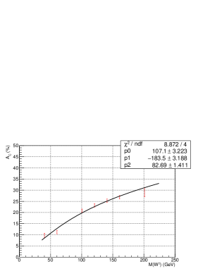
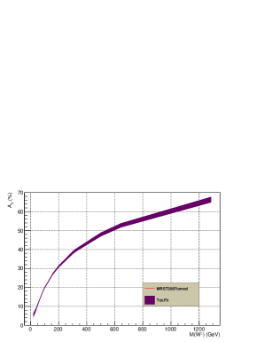
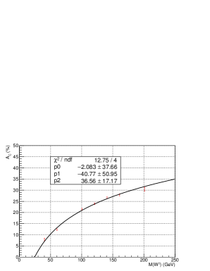
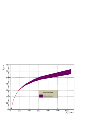
Figure 6: The $A_{C}^{Meas}$ template curves for the electron channel (top) and the muon channel (bottom). The fits to the $A^{Meas}_{C}(S)$ are presented on the LHS. These fits with uncertainty bands accounting for the correlation between the uncertainties of the fit parameters are shown on the RHS.

$Process$	$\alpha^{Exp}\pm\delta\alpha^{Stat}$	$Z_{N}$	$A_{C}^{Meas.}$	$\delta A_{C}^{Meas.}$	$\delta A_{C}^{Meas.Fit}$
		($\sigma$)	($\%$)	($\%$)	($\%$)
Signal: $W^{\pm}\to e^{\pm}\nu_{e}$
$M(W^{\pm})=40.2\rm\ GeV$	$(31.55\pm 0.77)\times 10^{-2}$	37.25	$9.66$	1.05	0.60
$M(W^{\pm})=60.3\rm\ GeV$	$(3.58\pm 0.07)\times 10^{-2}$	$>>5.00$	$11.22$	0.78	0.52
$M(W^{\pm})=\underline{80.4}\rm\ GeV$	$(2.74\pm 0.05)\times 10^{-2}$	$>>5.00$	$16.70$	0.76	0.35
$M(W^{\pm})=100.5\rm\ GeV$	$(3.13\pm 0.06)\times 10^{-2}$	$>>5.00$	$20.77$	0.77	0.33
$M(W^{\pm})=120.6\rm\ GeV$	$(3.89\pm 0.07)\times 10^{-2}$	$>>5.00$	$23.19$	0.78	0.35
$M(W^{\pm})=140.7\rm\ GeV$	$(4.82\pm 0.09)\times 10^{-2}$	$>>5.00$	$25.29$	0.78	0.39
$M(W^{\pm})=160.8\rm\ GeV$	$(6.00\pm 0.11)\times 10^{-2}$	$>>5.00$	$26.86$	0.79	0.42
$M(W^{\pm})=201.0\rm\ GeV$	$(88.77\pm 1.66)\times 10^{0}$	0.19	$29.07$	2.03	0.48

Table 8: Noise to signal ratio, signal statistical significance, and expected and measured integral charge asymmetries for the signal after the event selection in the electron channel.

The values of the noise to signal ratio ($\alpha^{Exp}$), the signal statistical significance ($Z_{N}$, defined in the next paragraph), the expected ($A_{C}^{Exp}$), and the measured ($A_{C}^{Meas}$) integral charge asymmetries for the signal after the event selection in the electron channel are reported in table 8.

The signal significances reported are calculated using a conversion of the confidence level of the signal plus background hypothesis $CL_{S+B}$ into an equivalent number of one-sided gaussian standard deviations $Z_{N}$ as proposed in 2006sppp.conf..112C and implemented in RooStats RooStats:Zn . For these calculations the systematic uncertainty of the background was set to $5\%$, which completely covers the total uncertainty for the measurement of the inclusive cross section $\sigma(p+p\to W^{\pm}\to\ell^{\pm}\nu)$ as reported in CMS:2011aa .

We recalculate the uncertainty on $A_{C}^{Meas}(S)$ accounting for the correlation between the parameters when fitting the $A_{C}^{Meas}(S)$ template curve by applying equation 15. This results in a slightly reduced uncertainty as shown in equation 19.

$$A_{C}^{Meas.Fit}(S)=(16.70\pm 0.35)\%$$ (19)

2.2.4. b. The Muon Channel

2.2.4. b.1. Event Selection in the Muon Channel

The following cuts are applied:

• $p_{T}(\mu)>20\rm\ GeV$

• $|\eta(\mu)|<2.4$

• Tracker Isolation: reject events with additional tracks of $p_{T}>2$ GeV within a cone of $\Delta R=0.5$ around the direction of the $\mu^{\pm}$ track

• Calorimeter Isolation: the ratio of, the scalar sum of $E_{T}$ deposits in the calorimeter within a cone of $\Delta R=0.5$ around the direction of the $\mu^{\pm}$, to the $p_{T}(\mu^{\pm})$ must be less than 0.25

• $\hbox to0.0pt{\kern 2.5pt/\hss}E_{T}>25\rm\ GeV$

• $M_{T}>40\rm\ GeV$

• Reject events with an additional trailing isolated muon: $\mu^{\pm}_{2}$

• Reject events with an additional leading isolated electron: $e^{\pm}_{1}$

• Reject events with an additional second track ($Track_{2}$) such that :

  $$\begin{cases}Q(\mu^{\pm}_{1})=-Q(Track_{2})\\ 3<p_{T}(Track_{2})<10\rm\ GeV\\ M[\mu_{1}^{\pm},Track_{2}]>50\rm\ GeV\end{cases}$$

The corresponding selection efficiencies and event yields are reported in table 9. The RHS of figure 5 displays the $\hbox to0.0pt{\kern 2.5pt/\hss}E_{T}$ distribution after the event selection. The non-resonant background processes represent $\sim 3\%$ of the total background after the event selection.

$Process$	$\epsilon$	$N_{exp}$	$A_{C}(S)\pm\delta A_{C}^{Stat}(S)$
	($\%$)	(k evts)	($\%$)
Signal: $W^{\pm}\to\mu^{\pm}\nu_{\mu}$
$M(W^{\pm})=40.2\rm\ GeV$	$1.22\pm 0.02$	439.192	$7.86\pm 1.28$
$M(W^{\pm})=60.3\rm\ GeV$	$12.27\pm 0.05$	2295.224	$12.30\pm 0.40$
$M(W^{\pm})=\underline{80.4}\rm\ GeV$	$29.32\pm 0.04$	3313.642	$17.42\pm 0.18$
$M(W^{\pm})=100.5\rm\ GeV$	$54.03\pm 0.07$	4034.779	$21.48\pm 0.19$
$M(W^{\pm})=120.6\rm\ GeV$	$31.30\pm 0.07$	1645.675	$23.93\pm 0.25$
$M(W^{\pm})=140.7\rm\ GeV$	$33.71\pm 0.07$	1316.121	$26.56\pm 0.23$
$M(W^{\pm})=160.8\rm\ GeV$	$35.37\pm 0.07$	1053.514	$27.90\pm 0.23$
$M(W^{\pm})=201.0\rm\ GeV$	$82.84\pm 0.05$	1.568	$30.44\pm 0.15$
Background	-	$277.787\pm 21.555$	$7.36\pm 0.15$
$W^{\pm}\to e^{\pm}\nu_{e}/\tau^{\pm}\nu_{\tau}/q\bar{q\prime}$	$0.291\pm 0.003$	177.500	$8.70\pm 1.07$
$t\bar{t}$	$4.27\pm 0.02$	4.895	$-0.14\pm 0.43$
$t+b,\ t+q(+b)$	$0.485\pm 0.005$	0.264	$27.14\pm 0.96$
$W+W,\ W+\gamma^{*}/Z,\ \gamma^{*}/Z+\gamma^{*}/Z$	$3.25\pm 0.01$	2.478	$11.39\pm 0.33$
$\gamma+\gamma,\ \gamma+jets,\ \gamma+W^{\pm},\ \gamma+Z$	$0.135\pm 0.001$	0.497	$17.48\pm 0.65$
$\gamma^{*}/Z$	$0.727\pm 0.001$	43.382	$5.79\pm 0.20$
QCD HF	$(2.13\pm 0.37)\times 10^{-4}$	17.983	$-17.65\pm 16.88$
QCD LF	$(1.38\pm 0.41)\times 10^{-4}$	30.788	$9.09\pm 30.03$

Table 9: Event selection efficiencies, event yields and integral charge asymmetries for the $W^{\pm}\to\mu^{\pm}\nu_{\mu}$ analysis.

2.2.4. b.2. The Measured $A_{C}$ in the Muon Channel

The $A_{C}^{Meas}(S)$ treatment described in paragraph 2.2.4. a.2. is applied to the probe sample in the muon channel, starting from the following inputs:

• $A_{C}^{Exp}(S)=(17.42\pm 0.18)\%$

• $A_{C}^{Exp}(B)=(7.36\pm 0.15)\%$

• $A_{C}^{Exp}(S+B)=(16.64\pm 0.12)\%$

• $\alpha^{Exp}=(8.38\pm 0.65)\times 10^{-2}$

For the nominal W mass, this leads to a measured integral charge asymmetry of:

$$A_{C}^{Meas}(S)=(17.42\pm 0.34)\%$$ (20)

where the uncertainty is also dominated by the value in equation 11.

2.2.4. b.3. The Template Curve in the Muon Channel

After applying the $A_{C}^{Meas}(S)$ treatment to the tag samples in the muon channel, we get the $A_{C}^{Meas}(S)$ template curve shown in the RHS of figure 6. The fit to this template curve is reported in equation 21.

$$A_{C}^{Meas}(W^{\pm}\to\mu^{\pm}\nu_{\mu})=-2.08-40.77\times Log(Log(M_{W^{\pm}}))+36.56\times Log(Log(M_{W^{\pm}}))^{2}$$ (21)

The values of the noise to signal ratio ($\alpha^{Exp}$), the signal statistical significance ($Z_{N}$), and the expected ($A_{C}^{Exp}$) and the measured ($A_{C}^{Meas}$) integral charge asymmetries for the signal after the event selection in the muon channel are reported in table 10.

$Process$	$\alpha^{Exp}\pm\delta\alpha^{Stat}$	$Z_{N}$	$A_{C}^{Meas.}$	$\delta A_{C}^{Meas.}$	$\delta A_{C}^{Meas.Fit}$
		($\sigma$)	($\%$)	($\%$)	($\%$)
Signal: $W^{\pm}\to\mu^{\pm}\nu_{\mu}$
$M(W^{\pm})=40.2\rm\ GeV$	$(63.25\pm 4.97)\times 10^{-2}$	11.19	7.86	0.59	0.45
$M(W^{\pm})=60.3\rm\ GeV$	$(12.10\pm 0.94)\times 10^{-2}$	2295.22	12.30	0.37	0.27
$M(W^{\pm})=\underline{80.4}\rm\ GeV$	$(8.38\pm 0.65)\times 10^{-2}$	3313.64	17.42	0.34	0.27
$M(W^{\pm})=100.5\rm\ GeV$	$(6.88\pm 0.53)\times 10^{-2}$	4034.78	21.48	0.35	0.22
$M(W^{\pm})=120.6\rm\ GeV$	$(16.88\pm 1.31)\times 10^{-2}$	1645.68	23.93	0.40	0.19
$M(W^{\pm})=140.7\rm\ GeV$	$(21.11\pm 1.64)\times 10^{-2}$	1316.12	26.56	0.42	0.22
$M(W^{\pm})=160.8\rm\ GeV$	$(26.37\pm 2.05)\times 10^{-2}$	1053.51	27.90	0.45	0.27
$M(W^{\pm})=201.0\rm\ GeV$	$(17.72\pm 1.37)\times 10^{1}$	1.57	30.44	0.87	0.40

Table 10: Noise to signal ratio, signal statistical significance, and expected and measured integral charge asymmetries for the signal after the event selection in the muon channel.

Again, accounting for the correlation between the parameters when fitting the $A_{C}^{Meas}(S)$ template curve enables to reduce the uncertainty as shown in equation 22.

$$A_{C}^{Meas.Fit}(S)=(17.42\pm 0.27)\%$$ (22)

2.3 Indirect Determination of $M_{W^{\pm}}$

2.3.1 Results in the Individual Channels

The $A_{C}^{Meas}(S)\pm\delta A_{C}^{Meas.Fit}(S)$ in the electron and in the muon channels translate into indirect $M^{Meas.Fit}_{W^{\pm}}\pm\delta M_{W^{\pm}}$ measurements using the experimental $A_{C}$ template curves from the RHS of figure 6 in each of these channels:

$$A_{C}^{Meas.Fit}(S)=(16.70\pm 0.35)\%\Rightarrow M^{Meas.Fit}(W^{\pm}\to e^{\pm}\nu_{e})=81.07^{+2.06}_{-2.01}\rm\ GeV,$$ (23)

$$A_{C}^{Meas.Fit}(S)=(17.42\pm 0.27)\%\Rightarrow M^{Meas.Fit}(W^{\pm}\to\mu^{\pm}\nu_{\mu})=79.67^{+3.56}_{-1.39}\rm\ GeV.$$ (24)

2.3.2 Combination of the Electron and the Muon Channels

We combine the electron and muon channels using a weighted mean for the measured $W^{\pm}$ mass, the weight is the inverse of the uncertainty on the measured mass. In order to account for the asymmetric uncertainties, we slightly modify the expressions for the weighted mean and the weighted RMS of a quantity $x$ as follows:

$$<x>=\frac{\sum_{i=1}^{N}\frac{x_{i}}{\delta^{2}_{i}}}{\sum_{i=1}^{N}\frac{1}{\delta^{2}_{i}}}\rm\ \ \ \to\rm\ \ \ <x>=\frac{\sum_{i=1}^{N}[\frac{x_{i}}{(\delta^{Up}_{i})^{2}}+\frac{x_{i}}{(\delta^{Down}_{i})^{2}}]}{\sum_{i=1}^{N}[\frac{1}{(\delta^{Up}_{i})^{2}}+\frac{1}{(\delta^{Down}_{i})^{2}}]}$$ (25)

$$\delta^{2}(<x>)=\frac{1}{\sum_{i=1}^{N}\frac{x_{i}}{\delta^{2}_{i}}}\rm\ \ \ \to\rm\ \ \ \delta^{2}(<x>)=\frac{1}{\sum_{i=1}^{N}[\frac{x_{i}}{(\delta^{Up}_{i})^{2}}+\frac{x_{i}}{(\delta^{Down}_{i})^{2}}]}$$ (26)

where $x_{i}$, $\delta^{Up}_{i}$ and $\delta^{Down}_{i}$ are respectively the central value, the upward uncertainty and the downward uncertainty of the mass derived in the channel $i$.

The result of the combination is:

$$M^{Comb.Meas.}(W^{\pm})=80.30\pm 0.96\rm\ GeV\rm\ [Expt.\ Comb.].$$ (27)

2.4 Final Result for MRST2007lomod

The next step is to estimate the theoretical uncertainty corresponding to the measured mass and to combine it with the experimental uncertainty. We simply use the central value of the measured $W^{\pm}$ mass and we read-off the theoretical template curve the intervals, defined by the intercepts with upper and lower fit curves.

$$M_{Theory}(W^{\pm})=80.30^{+0.19}_{-0.21}\rm\ GeV\rm\ [MRST2007lomod]$$ (28)

Finally we just sum in quadrature the theoretical and experimental upward and downward uncertainties:

$$\delta_{Tot.}M(W^{\pm})=80.30\begin{cases}+\sqrt{(0.96)^{2}+(0.19)^{2}}=&+0.98\\ -\sqrt{(0.96)^{2}+(0.21)^{2}}=&-0.98\end{cases}\rm\ GeV$$ (29)

Therefore the final result for the MRST2007lomod PDF reads:

$$M_{W^{\pm}}=80.30^{+0.98}_{-0.98}\rm\ GeV\ [Total\ MRST2007lomod].$$ (30)

This constitutes an indirect $M_{W^{\pm}}$ mesurement with a relative accuracy of $1.2\%$, where the experimental uncertainty largely dominates over the (underestimated) theoretical uncertainty.

2.5 Final Results for the Other Parton Density Functions

Since Delphes v1.9 does not store the set of variables $(x_{1},x_{2},flav_{1},flav_{2},Q^{2})$ necessary to access the PDF information from the generator, we slightly modify it so as to retrieve the
"HepMC::PdfInfo" object from the HepMC event record and to store it within the Delphes GEN branch as described in PDF-Info-Fix .

Based upon these variables we can apply PDF re-weightings so as to make experimental $A_{C}$ predictions for the CTEQ6L1 and the MSTW2008lo68cl PDFs. The new event weight is calculated in the standard way:

$$\rm PDFweight(New\ PDF)=\frac{f^{New\ PDF}_{Flav_{1}}(x_{1},Q^{2})}{f^{Old\ PDF}_{Flav_{1}}(x_{1},Q^{2})}\times\frac{f^{New\ PDF}_{Flav_{2}}(x_{2},Q^{2})}{f^{Old\ PDF}_{Flav_{2}}(x_{2},Q^{2})}$$ (31)

where the "Old PDF" is the default one, MRST2007lomod, and the "New PDF" is either CTEQ6L1 or MSTW2008lo68cl.

We re-run the electron and muon channel analyses and just change the weights of all the selected events. This results in signal event yields, and $A_{C}^{Exp}(S)$, $A_{C}^{Exp}(B)$ as reported in tables 11 and 12 for the CTEQ6L1 PDF and in tables 13 and 14 for the MSTW2008lo68cl one.

$\rm M_{W^{\pm}}$	$N_{Exp}(S)$	$A_{C}^{Exp}(S)$
(GeV)	(k Evts)	($\%$)
$40.2\ ^{e^{\pm}}_{\mu^{\pm}}$	${}^{288.688\pm 5.866}_{947.643\pm 11.535}$	${}^{11.26\pm 2.06}_{7.86\pm 1.28}$
$60.3\ ^{e^{\pm}}_{\mu^{\pm}}$	${}^{2491.955\pm 10.746}_{5285.294\pm 16.847}$	${}^{10.65\pm 0.49}_{12.30\pm 0.40}$
$80.4\ ^{e^{\pm}}_{\mu^{\pm}}$	${}^{3766.569\pm 8.423}_{5551.710\pm 6.752}$	${}^{15.78\pm 0.29}_{17.42\pm 0.18}$
$100.5\ ^{e^{\pm}}_{\mu^{\pm}}$	${}^{4106.984\pm 5.009}_{4188.292\pm 4.997}$	${}^{20.64\pm 0.19}_{21.48\pm 0.19}$
$120.6\ ^{e^{\pm}}_{\mu^{\pm}}$	${}^{2739.825\pm 4.796}_{3777.497\pm 4.730}$	${}^{23.54\pm 0.26}_{23.93\pm 0.25}$
$140.7\ ^{e^{\pm}}_{\mu^{\pm}}$	${}^{2284.590\pm 3.512}_{3020.544\pm 3.268}$	${}^{25.52\pm 0.25}_{26.56\pm 0.23}$
$160.8\ ^{e^{\pm}}_{\mu^{\pm}}$	${}^{1584.146\pm 2.512}_{2461.819\pm 2.255}$	${}^{27.07\pm 0.24}_{27.90\pm 0.23}$
$201.0\ ^{e^{\pm}}_{\mu^{\pm}}$	${}^{1.259\pm 0.002}_{1.628\pm 0.001}$	${}^{29.57\pm 0.23}_{30.64\pm 0.15}$

Table 11: Number of expected signal events and expected signal $A_{C}$ as a function of $M(W^{\pm})$ for the electron and muon analyses reweighted to the CTEQ6L1 PDF predictions.

$W^{\pm}$ Decay Channel	$N_{Exp}(B)$	$A_{C}^{Exp}(B)$
	(k Evts)	($\%$)
$e^{\pm}$	$352.660\pm 7.996$	$9.74\pm 0.23$
$\mu^{\pm}$	$707.617\pm 29.944$	$7.45\pm 0.15$

Table 12: Number of expected background events and expected background $A_{C}$ for the electron (upper line) and the muon (lower line) analyses reweighted to the CTEQ6L1 PDF predictions.

Then we produce the experimental $A_{C}$ template curves for CTEQ6L1 and MSTW2008lo68cl and both analysis channels as displayed in figures 7 and 8.

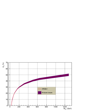
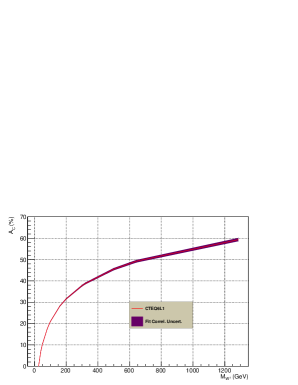
Figure 7: The CTEQ6L1 $A_{C}$ template curves for the $W^{\pm}\to e^{\pm}\nu_{e}$ (top) and the $W^{\pm}\to\mu^{\pm}\nu_{\mu}$ (bottom) analyses. The fits to the $A^{Exp}_{C}(S)$ are presented on the LHS. These fits with uncertainty bands accounting for the correlation between the uncertainties of the fit parameters are shown on the RHS.

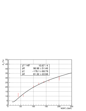
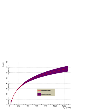
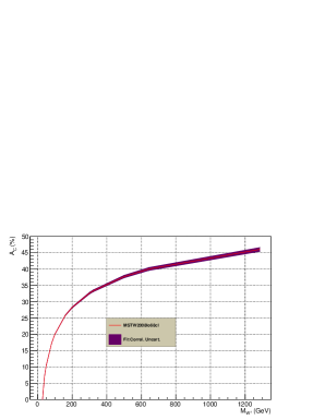
Figure 8: The MSTW2008lo68cl $A_{C}$ template curves for the $W^{\pm}\to e^{\pm}\nu_{e}$ (top) and the $W^{\pm}\to\mu^{\pm}\nu_{\mu}$ (bottom) analyses. The fits to the $A^{Exp}_{C}(S)$ are presented on the LHS. These fits with uncertainty bands accounting for the correlation between the uncertainties of the fit parameters are shown on the RHS.

For the CTEQ6L1 PDF, we find:

$$A_{C}^{Meas.Fit}(S)=(15.78\pm 0.50)\%\Rightarrow M^{Meas}(W^{\pm}\to e^{\pm}\nu_{e})=73.39^{+2.40}_{-2.30}\rm\ GeV,$$ (32)

$$A_{C}^{Meas.Fit}(S)=(17.42\pm 0.18)\%\Rightarrow M^{Meas}(W^{\pm}\to\mu^{\pm}\nu_{\mu})=79.82^{+0.94}_{-0.92}\rm\ GeV$$ (33)

which leads to the following combined value:

$$M^{Comb.Meas.}(W^{\pm}\to\ell^{\pm}\nu_{\ell})=(78.95\pm 0.61)\rm\ GeV\ [Expt.\ CTEQ6L1]$$ (34)

To this measured central value of the mass correspond the following theoretical uncertainties:

$$M(W^{\pm})=78.95^{+0.11}_{-0.13}\rm\ GeV\rm\ [Theory\ CTEQ6L1],$$ (35)

Therefore the final result for the CTEQ6L1 PDF reads:

$$M(W^{\pm})=78.95^{+0.62}_{-0.62}\rm\ GeV\rm\ [Total\ CTEQ6L1]$$ (36)

and it’s dominant uncertainty is also experimental, since its theoretical uncertainty is underestimated. This represents an indirect measurement of the $W^{\pm}$ mass with a relative accuracy of $0.8\%$.

$\rm M_{W^{\pm}}$	$N_{Exp}(S)$	$A_{C}^{Exp}(S)$
(GeV)	(k Evts)	($\%$)
$40.2\ ^{e^{\pm}}_{\mu^{\pm}}$	${}^{280.257\pm 5.781}_{913.868\pm 11.334}$	${}^{11.26\pm 2.06}_{7.86\pm 1.28}$
$60.3\ ^{e^{\pm}}_{\mu^{\pm}}$	${}^{2469.515\pm 10.705}_{5219.408\pm 16.783}$	${}^{10.65\pm 0.49}_{12.30\pm 0.40}$
$80.4\ ^{e^{\pm}}_{\mu^{\pm}}$	${}^{3663.615\pm 8.363}_{5711.468\pm 6.753}$	${}^{15.78\pm 0.29}_{17.42\pm 0.18}$
$100.5\ ^{e^{\pm}}_{\mu^{\pm}}$	${}^{4053.288\pm 5.016}_{4165.175\pm 5.000}$	${}^{20.64\pm 0.19}_{21.48\pm 0.19}$
$120.6\ ^{e^{\pm}}_{\mu^{\pm}}$	${}^{2665.994\pm 4.800}_{3811.380\pm 4.697}$	${}^{23.54\pm 0.26}_{23.93\pm 0.25}$
$140.7\ ^{e^{\pm}}_{\mu^{\pm}}$	${}^{2221.101\pm 3.530}_{3033.091\pm 3.252}$	${}^{25.52\pm 0.25}_{26.56\pm 0.23}$
$160.8\ ^{e^{\pm}}_{\mu^{\pm}}$	${}^{1539.501\pm 2.516}_{2446.996\pm 2.280}$	${}^{27.07\pm 0.24}_{27.90\pm 0.23}$
$201.0\ ^{e^{\pm}}_{\mu^{\pm}}$	${}^{1.230\pm 0.002}_{1.645\pm 0.001}$	${}^{29.57\pm 0.23}_{30.64\pm 0.15}$

Table 13: Number of expected signal events and expected signal $A_{C}$ as a function of $M(W^{\pm})$ for the electron and muon analyses reweighted to the MSTW2008lo68cl PDF predictions.

For the MSTW2008lo68cl PDF:

$W^{\pm}$ Decay Channel	$N_{Exp}(B)$	$A_{C}^{Exp}(B)$
	(k Evts)	($\%$)
$e^{\pm}$	$371.956\pm 8.081$	$9.74\pm 0.23$
$\mu^{\pm}$	$721.196\pm 29.968$	$7.45\pm 0.15$

Table 14: Number of expected background events and expected background $A_{C}$ for the electron (upper line) and muon (lower line) analyses reweighted to the MSTW2008lo68cl PDF predictions.

$$A_{C}^{Meas.Fit}(S)=(15.78\pm 0.52)\%\Rightarrow M^{Meas}(W^{\pm}\to e^{\pm}\nu_{e})=76.91^{+2.80}_{-2.74}\rm\ GeV,$$ (37)

$$A_{C}^{Meas.Fit}(S)=(17.42\pm 0.18)\%\Rightarrow M^{Meas}(W^{\pm}\to\mu^{\pm}\nu_{\mu})=82.07^{+1.11}_{-1.10}\rm\ GeV$$ (38)

which leads to the following combined value:

$$M^{Comb.Meas.}(W^{\pm}\to\ell^{\pm}\nu_{\ell})=(81.36\pm 0.73)\rm\ GeV$$ (39)

The corresponding theoretical uncertainties are:

$$M(W^{\pm})=81.36^{+1.50}_{-1.32}\rm\ GeV\rm\ [Theory\ MSTW2008lo68cl],$$ (40)

Therefore the final result for the MSTW2008lo68cl PDF reads:

$$M(W^{\pm})=81.36^{+1.67}_{-1.51}\rm\ GeV\rm\ [Total\ MSTW2008lo68cl]$$ (41)

and it’s dominant uncertainty comes from $\delta^{Theory}_{PDF}A_{C}$ . In this case, this represents an indirect measurement of the $W^{\pm}$ mass with a relative accuracy of $2.1\%$.

2.6 Summary of the $M_{W^{\pm}}$ Measurements and their Accuracy

We sum up the indirect mass measurements of $M_{W^{\pm}}$ extracted from the integral charge asymmetry of the $W^{\pm}\to\ell^{\pm}\nu$ inclusive process within table 15. Therein we also present a few figures of merit of the accuracy of these measurements:

1. $\frac{\delta M^{Fit}_{W^{\pm}}}{M^{Fit}_{W^{\pm}}}$

2. $\frac{(M^{Fit}_{W^{\pm}}-M^{True}_{W^{\pm}})}{M^{True}_{W^{\pm}}}$

3. $\frac{(M^{Fit}_{W^{\pm}}-M^{True}_{W^{\pm}})}{\delta M^{Fit}_{W^{\pm}}}$

In this notation, $M^{Fit}_{W^{\pm}}$ and $\delta M^{Fit}_{W^{\pm}}$ represent the indirectly measured $M_{W^{\pm}}$ and its uncertainty, and $M^{True}_{W^{\pm}}$ stands for the nominal $W^{\pm}$ boson mass.

The first figure of merit (1.) reflects the intrinsic resolution power of the indirect mass measurement, irrespective of its possible biases, it’s expressed in $\%$. The second and the third ones measure the accuracy with respect to the nominal $W^{\pm}$ boson mass: firstly as a relative uncertainty in $\%$ irrespective of the precision of the method (2.) and secondly as a compatibility between the nominal and the predicted masses given the precision of the method (3.), expressed in number of standard deviations ($\sigma$).

Figures of Merit	Considered LO PDFs
of the Accuracy	MRST2007lomod	CTEQ6L1	MSTW2008lo68cl
1. $\frac{\delta M^{Fit}_{W^{\pm}}}{M^{Fit}_{W^{\pm}}}$	$1.2\%$	$0.8\%$	$2.1\%$
2. $\frac{(M^{Fit}_{W^{\pm}}-M^{True}_{W^{\pm}})}{M^{True}_{W^{\pm}}}$	$-0.1\%$	$-1.8\%$	$+1.2\%$
3. $\frac{(M^{Fit}_{W^{\pm}}-M^{True}_{W^{\pm}})}{\delta M^{Fit}_{W^{\pm}}}$	$-0.1\sigma$	$-2.3\sigma$	$+0.6\sigma$

Table 15: Summary of the indirect mass measurements of $M_{W^{\pm}}$ extracted from the integral charge asymmetry of the $W^{\pm}\to\ell^{\pm}\nu$ process. Different figures of merit of the accuracy of these measurements are presented.

The values of the figures of merit in table 15 show that already at LO, this new method enables to get a good estimate of the $W^{\pm}$ boson mass.

3 Inclusive Production of $\tilde{\chi}^{\pm}_{1}+\tilde{\chi}^{0}_{2}\to 3\ell^{\pm}+\hbox to0.0pt{\kern 2.5pt/\hss}E_{T}$

3.1 Theoretical Prediction of $A_{C}(\tilde{\chi}^{\pm}_{1}+\tilde{\chi}^{0}_{2})$

In this section we repeat the types of calculations done in section 2.1 but now for a process of interest in R-parity conserving SUSY searches, namely the $p+p\to\tilde{\chi}^{\pm}_{1}+\tilde{\chi}^{0}_{2}\to 3\ell^{\pm}+\hbox to0.0pt{\kern 2.5pt/\hss}E_{T}$ inclusive production.

We use Resummino v1.0.0 Fuks:2013vua to calculate the $p+p\to\tilde{\chi}^{\pm}_{1}+\tilde{\chi}^{0}_{2}$ cross sections at different levels of theoretical accuracy. At fixed order in QCD we run these calculations at the LO and the NLO. In addition, we also run them starting from the NLO MEs and including the "Next-to-Leading Log" (NLL) analytically resummed corrections. The latter, sometimes refered to as "NLO+NLL" will simply be denoted "NLL" in the following.

We calculate these cross sections at $\sqrt{s}=8$ TeV using "Simplified Models" Alwall:2008ag for the following masses:

$$M_{\tilde{\chi}^{\pm}_{1}}=M_{\tilde{\chi}^{0}_{2}}=100,105,115,125,135,145,150,200,250,300,400,500,600,700\rm\ GeV$$

and using the PDFs reported in table 16. We set the QCD scales as $\mu_{R}=\mu_{F}=\mu_{0}=M_{\tilde{\chi}^{\pm}_{1}}+M_{\tilde{\chi}^{0}_{2}}$. Regarding the phase space sampling, a statistical precision of $0.1\%$ is requested for the numerical integration of the cross sections.

LO	NLO $\&$ NLL
MRST2007lomod	MRST2004nlo
CTEQ6L1	CTEQ6.1
MSTW2008lo68cl	MSTW2008nlo68cl

Table 16: PDFs used for the calculations of $\sigma(\tilde{\chi}^{\pm}_{1}+\tilde{\chi}^{0}_{2})$ at the LO in QCD and the NLO and the NLL.

The integral charge asymmetries as functions of $M_{\tilde{\chi}^{\pm}_{1}}+M_{\tilde{\chi}^{0}_{2}}$ for this process are presented in tables 17, 19, and 21 for the MRST2007lomod/MRST2004nlo, the CTEQ6L1/CTEQ61, and the MSTW2008lo68cl/MSTW2008nlo68cl PDFs, respectively.

3.1.1 $A_{C}(\tilde{\chi}^{\pm}_{1}+\tilde{\chi}^{0}_{2})$ Template Curves for MRST

The theoretical MRST $A_{C}$ template curves are obtained by computing the $A_{C}$ based upon the cross sections of the signed processes used for table 17. They are displayed in figure 9.

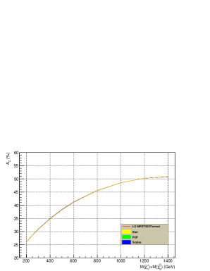
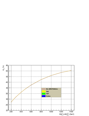
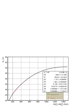
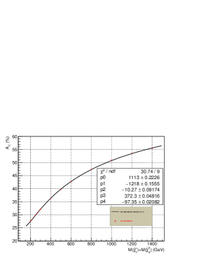
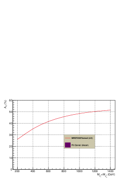
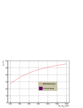
Figure 9: The theoretical MRST $A_{C}$ template curves. The raw curve with its uncertainty bands and the corresponding fitted curve wtih uncorrelated and with correlated uncertainties are displayed on the top, the middle and the bottom rows, respectively. The LHS concerns the LO calculations based upon the MRST2007lomod PDF and the RHS concerns the NLL calculations using the MRST2004nlo PDF.

$\rm M_{\chi^{\pm}_{1}}+M_{\chi^{0}_{2}}$	$A_{C}$	$\delta(A_{C})_{Stat}$	$\delta(A_{C})_{Scale}$	$\delta(A_{C})_{PDF}$	$\delta(A_{C})_{Total}$
(GeV)	($\%$)	($\%$)	($\%$)	($\%$)	($\%$)
200.	LO: 25.991	$\pm 0.004$	${}^{-0.037}_{+0.056}$	0.000	${}^{+0.037}_{-0.056}$
	NLL: 27.363	$\pm 0.011$	${}^{+0.092}_{-0.074}$	not quoted	${}^{+0.093}_{-0.075}$
210.	LO: 26.52	$\pm 0.003$	${}^{-0.046}_{+0.063}$	0.000	${}^{+0.046}_{-0.063}$
	NLL: 27.904	$\pm 0.009$	${}^{+0.100}_{-0.066}$	not quoted	${}^{+0.101}_{-0.067}$
230.	LO: 27.562	$\pm 0.002$	${}^{-0.061}_{+0.074}$	0.000	${}^{+0.061}_{-0.074}$
	NLL: 28.938	$\pm 0.006$	${}^{+0.098}_{-0.056}$	not quoted	${}^{+0.099}_{-0.057}$
250.	LO: 28.549	$\pm 0.002$	${}^{-0.073}_{+0.085}$	0.000	${}^{+0.074}_{-0.085}$
	NLL: 29.934	$\pm 0.004$	${}^{+0.084}_{-0.072}$	not quoted	${}^{+0.084}_{-0.073}$
270.	LO: 29.495	$\pm 0.001$	${}^{-0.084}_{+0.094}$	0.000	${}^{+0.084}_{-0.094}$
	NLL: 30.877	$\pm 0.003$	${}^{+0.085}_{-0.088}$	not quoted	${}^{+0.085}_{-0.088}$
290.	LO: 30.403	$\pm 0.001$	${}^{-0.094}_{+0.102}$	0.000	${}^{+0.094}_{-0.102}$
	NLL: 31.786	$\pm 0.002$	${}^{+0.079}_{-0.091}$	not quoted	${}^{+0.079}_{-0.091}$
300.	LO: 30.844	$\pm 0.001$	${}^{-0.098}_{+0.106}$	0.000	${}^{+0.098}_{-0.106}$
	NLL: 32.229	$\pm 0.002$	${}^{+0.076}_{-0.093}$	not quoted	${}^{+0.076}_{-0.093}$
400.	LO: 34.847	$\pm 0.000$	${}^{-0.125}_{+0.126}$	0.000	${}^{+0.125}_{-0.126}$
	NLL: 36.213	$\pm 0.001$	${}^{+0.086}_{-0.069}$	not quoted	${}^{+0.086}_{-0.069}$
500.	LO: 38.230	$\pm 0.000$	${}^{-0.132}_{+0.131}$	0.000	${}^{+0.132}_{-0.131}$
	NLL: 39.648	$\pm 0.000$	${}^{+0.101}_{-0.100}$	not quoted	${}^{+0.101}_{-0.100}$
600.	LO: 41.101	$\pm 0.000$	${}^{-0.127}_{+0.124}$	0.000	${}^{+0.127}_{-0.124}$
	NLL: 42.600	$\pm 0.000$	${}^{+0.104}_{-0.129}$	not quoted	${}^{+0.104}_{-0.129}$
800.	LO: 45.548	$\pm 0.000$	${}^{-0.091}_{+0.086}$	0.000	${}^{+0.091}_{-0.086}$
	NLL: 47.420	$\pm 0.000$	${}^{+0.118}_{-0.073}$	not quoted	${}^{+0.118}_{-0.073}$
1000.	LO: 48.528	$\pm 0.000$	${}^{-0.038}_{+0.033}$	0.000	${}^{+0.038}_{-0.033}$
	NLL: 51.035	$\pm 0.000$	${}^{+0.116}_{-0.063}$	not quoted	${}^{+0.116}_{-0.063}$
1200.	LO: 50.264	$\pm 0.000$	${}^{+0.024}_{-0.025}$	0.000	${}^{+0.024}_{-0.025}$
	NLL: 53.658	$\pm 0.000$	${}^{+0.101}_{+0.021}$	not quoted	${}^{+0.101}_{-0.021}$
1400.	LO: 50.924	$\pm 0.000$	${}^{+0.088}_{-0.081}$	0.000	${}^{+0.088}_{-0.081}$
	NLL: 55.404	$\pm 0.000$	${}^{+0.008}_{-0.083}$	not quoted	${}^{+0.008}_{-0.083}$

Table 17: The MRST $A_{C}(\tilde{\chi}^{\pm}_{1}\tilde{\chi}^{0}_{2})$ table with the breakdown of the different sources of theoretical uncertainty.

$\rm M_{\chi^{\pm}_{1}}+M_{\chi^{0}_{2}}\ (GeV)$	$A_{C}^{Fit}$	$\delta A^{Fit}_{C}$
(GeV)	($\%$)	($\%$)
200.	LO: 25.984	$\pm 0.025$
	NLL: 27.435	$\pm 0.031$
210.	LO: 26.530	$\pm 0.024$
	NLL: 27.927	$\pm 0.030$
230.	LO: 27.571	$\pm 0.024$
	NLL: 28.904	$\pm 0.028$
250.	LO: 28.557	$\pm 0.023$
	NLL: 29.866	$\pm 0.027$
270.	LO: 29.498	$\pm 0.023$
	NLL: 30.807	$\pm 0.027$
290.	LO: 30.400	$\pm 0.022$
	NLL: 31.724	$\pm 0.026$
300.	LO: 30.838	$\pm 0.022$
	NLL: 32.172	$\pm 0.026$
400.	LO: 34.824	$\pm 0.021$
	NLL: 36.286	$\pm 0.025$
500.	LO: 38.215	$\pm 0.020$
	NLL: 39.768	$\pm 0.027$
600.	LO: 41.102	$\pm 0.019$
	NLL: 42.720	$\pm 0.029$
800.	LO: 45.562	$\pm 0.016$
	NLL: 47.400	$\pm 0.034$
1000.	LO: 48.532	$\pm 0.015$
	NLL: 50.881	$\pm 0.041$
1200.	LO: 50.261	$\pm 0.017$
	NLL: 53.508	$\pm 0.049$
1400.	LO: 50.945	$\pm 0.022$
	NLL: 55.501	$\pm 0.057$

Table 18: The MRST $A_{C}^{Fit}(\tilde{\chi}^{\pm}_{1}\tilde{\chi}^{0}_{2})$ table with its theoretical uncertainty accounting for the correlations between the parameters fitting the $A_{C}^{Raw}$ template curves.

3.1.2 $A_{C}(\tilde{\chi}^{\pm}_{1}+\tilde{\chi}^{0}_{2})$ Template Curves for CTEQ6

The theoretical CTEQ6 $A_{C}$ template curves are obtained by computing the $A_{C}$ based upon the cross sections of the signed processes used for table 19. They are displayed in figure 10.

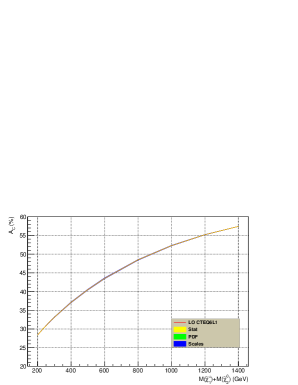
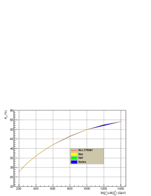
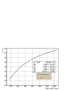
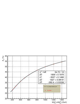
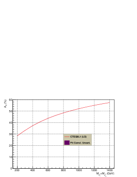
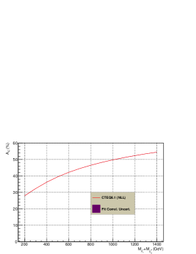
Figure 10: The theoretical CTEQ6 $A_{C}$ template curves. The raw curve with its uncertainty bands and the corresponding fitted curve wtih uncorrelated and with correlated uncertainties are displayed on the top, the middle and the bottom rows, respectively. The LHS concerns the LO calculations based upon the CTEQ6L1 PDF and the RHS concerns the NLL calculations using the CTEQ6.1 PDF.

$\rm M_{\chi^{\pm}_{1}}+M_{\chi^{0}_{2}}$	$A_{C}$	$\delta(A_{C})_{Stat}$	$\delta(A_{C})_{Scale}$	$\delta(A_{C})_{PDF}$	$\delta(A_{C})_{Total}$
(GeV)	($\%$)	($\%$)	($\%$)	($\%$)	($\%$)
200.	LO: 28.367	$\pm 0.003$	${}^{-0.030}_{+0.045}$	0.000	${}^{+0.030}_{-0.045}$
	NLL: 27.822	$\pm 0.010$	${}^{+0.076}_{-0.074}$	not quoted	${}^{+0.077}_{-0.075}$
210.	LO: 28.896	$\pm 0.003$	${}^{-0.038}_{+0.051}$	0.000	${}^{+0.038}_{-0.051}$
	NLL: 28.345	$\pm 0.008$	${}^{+0.084}_{-0.069}$	not quoted	${}^{+0.084}_{-0.069}$
230.	LO: 29.911	$\pm 0.002$	${}^{-0.053}_{+0.064}$	0.000	${}^{+0.053}_{-0.064}$
	NLL: 29.333	$\pm 0.006$	${}^{+0.102}_{-0.054}$	not quoted	${}^{+0.102}_{-0.054}$
250.	LO: 30.880	$\pm 0.001$	${}^{-0.066}_{+0.074}$	0.000	${}^{+0.066}_{+0.074}$
	NLL: 30.273	$\pm 0.004$	${}^{+0.093}_{-0.064}$	not quoted	${}^{+0.093}_{-0.064}$
270.	LO: 31.808	$\pm 0.001$	${}^{-0.077}_{+0.084}$	0.000	${}^{+0.077}_{-0.084}$
	NLL: 31.169	$\pm 0.003$	${}^{+0.078}_{-0.070}$	not quoted	${}^{+0.078}_{-0.070}$
290.	LO: 32.701	$\pm 0.001$	${}^{-0.087}_{+0.092}$	0.000	${}^{+0.087}_{-0.092}$
	NLL: 32.026	$\pm 0.002$	${}^{+0.065}_{-0.090}$	not quoted	${}^{+0.065}_{-0.090}$
300.	LO: 33.135	$\pm 0.001$	${}^{-0.091}_{+0.096}$	0.000	${}^{+0.091}_{-0.096}$
	NLL: 32.434	$\pm 0.002$	${}^{+0.065}_{-0.089}$	not quoted	${}^{+0.065}_{-0.089}$
400.	LO: 37.104	$\pm 0.000$	${}^{-0.121}_{+0.121}$	0.000	${}^{+0.121}_{-0.121}$
	NLL: 36.136	$\pm 0.001$	${}^{+0.080}_{-0.055}$	not quoted	${}^{+0.080}_{-0.055}$
500.	LO: 40.531	$\pm 0.000$	${}^{-0.134}_{+0.131}$	0.000	${}^{+0.134}_{-0.131}$
	NLL: 39.285	$\pm 0.000$	${}^{+0.088}_{-0.057}$	not quoted	${}^{+0.088}_{-0.057}$
600.	LO: 43.527	$\pm 0.000$	${}^{-0.137}_{+0.132}$	0.000	${}^{+0.137}_{-0.132}$
	NLL: 42.023	$\pm 0.000$	${}^{+0.056}_{-0.119}$	not quoted	${}^{+0.056}_{-0.119}$
800.	LO: 48.473	$\pm 0.000$	${}^{-0.121}_{+0.116}$	0.000	${}^{+0.121}_{-0.116}$
	NLL: 46.514	$\pm 0.000$	${}^{+0.094}_{-0.194}$	not quoted	${}^{+0.094}_{-0.194}$
1000.	LO: 52.293	$\pm 0.000$	${}^{-0.094}_{+0.090}$	0.000	${}^{+0.094}_{-0.090}$
	NLL: 49.985	$\pm 0.000$	${}^{+0.054}_{-0.053}$	not quoted	${}^{+0.054}_{-0.053}$
1200.	LO: 55.219	$\pm 0.000$	${}^{-0.063}_{+0.061}$	0.000	${}^{+0.063}_{-0.061}$
	NLL: 52.447	$\pm 0.000$	${}^{+0.528}_{+0.147}$	not quoted	${}^{+0.528}_{-0.147}$
1400.	LO: 57.428	$\pm 0.000$	${}^{-0.034}_{+0.033}$	0.000	${}^{+0.034}_{-0.033}$
	NLL: 54.190	$\pm 0.000$	${}^{+0.069}_{-0.081}$	not quoted	${}^{+0.069}_{-0.081}$

Table 19: The CTEQ6 $A_{C}(\tilde{\chi}^{\pm}_{1}\tilde{\chi}^{0}_{2})$ table with the breakdown of the different sources of theoretical uncertainty.

$\rm M_{\chi^{\pm}_{1}}+M_{\chi^{0}_{2}}\ (GeV)$	$A_{C}^{Fit}$	$\delta A^{Fit}_{C}$
(GeV)	($\%$)	($\%$)
200.	LO: 28.407	$\pm 0.034$
	NLL: 27.811	$\pm 0.027$
210.	LO: 28.900	$\pm 0.027$
	NLL: 28.340	$\pm 0.026$
230.	LO: 29.876	$\pm 0.023$
	NLL: 29.342	$\pm 0.024$
250.	LO: 30.832	$\pm 0.027$
	NLL: 30.282	$\pm 0.023$
270.	LO: 31.766	$\pm 0.032$
	NLL: 31.172	$\pm 0.022$
290.	LO: 32.674	$\pm 0.037$
	NLL: 32.018	$\pm 0.022$
300.	LO: 33.119	$\pm 0.038$
	NLL: 32.428	$\pm 0.022$
400.	LO: 37.203	$\pm 0.046$
	NLL: 36.126	$\pm 0.023$
500.	LO: 40.687	$\pm 0.048$
	NLL: 39.287	$\pm 0.026$
600.	LO: 43.675	$\pm 0.052$
	NLL: 42.041	$\pm 0.027$
800.	LO: 48.507	$\pm 0.058$
	NLL: 46.558	$\pm 0.030$
1000.	LO: 52.220	$\pm 0.052$
	NLL: 49.977	$\pm 0.033$
1200.	LO: 55.133	$\pm 0.034$
	NLL: 52.477	$\pm 0.041$
1400.	LO: 57.447	$\pm 0.032$
	NLL: 54.189	$\pm 0.052$

Table 20: The CTEQ $A_{C}^{Fit}(\tilde{\chi}^{\pm}_{1}\tilde{\chi}^{0}_{2})$ table with its theoretical uncertainty accounting for the correlations between the parameters fitting the $A_{C}^{Raw}$ template curves.

3.1.3 $A_{C}(\tilde{\chi}^{\pm}_{1}+\tilde{\chi}^{0}_{2})$ Template Curves for MSTW2008

The theoretical MSTW2008lo68cl $A_{C}$ template curves are obtained by computing the $A_{C}$ based upon the cross sections of the signed processes used for table 21. They are displayed in figure 11.

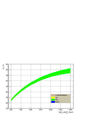
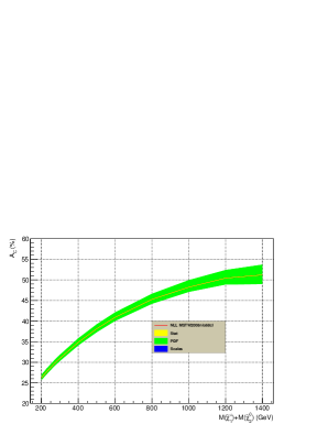
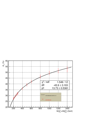
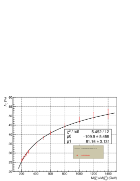
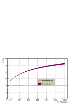
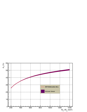
Figure 11: The theoretical MSTW2008 $A_{C}$ template curves. The raw curve with its uncertainty bands and the corresponding fitted curve wtih uncorrelated and with correlated uncertainties are displayed on the top, the middle and the bottom rows, respectively. The LHS concerns the LO calculations based upon the MSTW2008lo68cl PDF and the RHS concerns the NLL calculations using the MSTW2008nlo68cl PDF.

$\rm M_{\chi^{\pm}_{1}}+M_{\chi^{0}_{2}}$	$A_{C}$	$\delta(A_{C})_{Stat}$	$\delta(A_{C})_{Scale}$	$\delta(A_{C})_{PDF}$	$\delta(A_{C})_{Total}$
(GeV)	($\%$)	($\%$)	($\%$)	($\%$)	($\%$)
200.	LO: 27.330	$\pm 0.003$	${}^{-0.034}_{+0.049}$	${}^{+0.827}_{-0.649}$	${}^{+0.828}_{-0.651}$
	NLL: 26.215	$\pm 0.011$	${}^{+0.091}_{-0.067}$	${}^{+0.682}_{-0.518}$	${}^{+0.688}_{-0.522}$
210.	LO: 27.857	$\pm 0.003$	${}^{-0.042}_{+0.056}$	${}^{+0.845}_{-0.663}$	${}^{+0.846}_{-0.665}$
	NLL: 26.744	$\pm 0.009$	${}^{+0.080}_{-0.056}$	${}^{+0.694}_{-0.530}$	${}^{+0.698}_{-0.533}$
230.	LO: 28.872	$\pm 0.002$	${}^{-0.056}_{-0.068}$	${}^{+0.878}_{-0.690}$	${}^{+0.880}_{-0.693}$
	NLL: 27.757	$\pm 0.006$	${}^{+0.085}_{-0.040}$	${}^{+0.722}_{-0.549}$	${}^{+0.727}_{-0.550}$
250.	LO: 29.842	$\pm 0.001$	${}^{-0.069}_{+0.078}$	${}^{+0.911}_{-0.716}$	${}^{+0.913}_{-0.720}$
	NLL: 28.730	$\pm 0.004$	${}^{+0.073}_{-0.053}$	${}^{+0.747}_{-0.573}$	${}^{+0.751}_{-0.575}$
270.	LO: 30.770	$\pm 0.001$	${}^{-0.080}_{+0.087}$	${}^{+0.942}_{-0.742}$	${}^{+0.945}_{-0.747}$
	NLL: 29.658	$\pm 0.003$	${}^{+0.063}_{-0.069}$	${}^{+0.773}_{-0.595}$	${}^{+0.775}_{-0.599}$
290.	LO: 31.662	$\pm 0.001$	${}^{-0.088}_{+0.094}$	${}^{+0.972}_{-0.766}$	${}^{+0.976}_{-0.772}$
	NLL: 30.540	$\pm 0.002$	${}^{+0.058}_{-0.080}$	${}^{+0.802}_{-0.608}$	${}^{+0.804}_{-0.613}$
300.	LO: 32.096	$\pm 0.001$	${}^{-0.092}_{+0.097}$	${}^{+0.987}_{-0.778}$	${}^{+0.991}_{-0.784}$
	NLL: 30.969	$\pm 0.002$	${}^{+0.068}_{-0.089}$	${}^{+0.802}_{-0.625}$	${}^{+0.805}_{-0.632}$
400.	LO: 36.028	$\pm 0.000$	${}^{-0.117}_{+0.117}$	${}^{+1.123}_{-0.885}$	${}^{+1.129}_{-0.893}$
	NLL: 34.846	$\pm 0.001$	${}^{+0.105}_{-0.043}$	${}^{+0.929}_{-0.713}$	${}^{+0.935}_{-0.714}$
500.	LO: 39.351	$\pm 0.000$	${}^{-0.123}_{+0.122}$	${}^{+1.250}_{-0.971}$	${}^{+1.256}_{-0.979}$
	NLL: 38.145	$\pm 0.000$	${}^{+0.097}_{-0.093}$	${}^{+1.042}_{-0.803}$	${}^{+1.047}_{-0.808}$
600.	LO: 42.179	$\pm 0.000$	${}^{-0.118}_{+0.116}$	${}^{+1.372}_{-1.043}$	${}^{+1.377}_{-1.050}$
	NLL: 40.906	$\pm 0.000$	${}^{+0.121}_{-0.103}$	${}^{+1.171}_{-0.841}$	${}^{+1.177}_{-0.847}$
800.	LO: 46.628	$\pm 0.000$	${}^{-0.088}_{+0.085}$	${}^{+1.627}_{-1.161}$	${}^{+1.629}_{-1.164}$
	NLL: 45.265	$\pm 0.000$	${}^{+0.101}_{-0.080}$	${}^{+1.352}_{-1.027}$	${}^{+1.356}_{-1.030}$
1000.	LO: 49.793	$\pm 0.000$	${}^{-0.051}_{+0.046}$	${}^{+1.953}_{-1.242}$	${}^{+1.953}_{-1.243}$
	NLL: 48.243	$\pm 0.000$	${}^{+0.112}_{-0.019}$	${}^{+1.674}_{-1.124}$	${}^{+1.678}_{-1.125}$
1200.	LO: 51.956	$\pm 0.000$	${}^{-0.014}_{+0.013}$	${}^{+2.407}_{-1.301}$	${}^{+2.408}_{-1.301}$
	NLL: 50.430	$\pm 0.000$	${}^{+0.031}_{-0.000}$	${}^{+1.966}_{-1.534}$	${}^{+1.966}_{-1.534}$
1400.	LO: 53.328	$\pm 0.000$	${}^{+0.018}_{-0.013}$	${}^{+3.019}_{-1.375}$	${}^{+3.019}_{-1.375}$
	NLL: 51.216	$\pm 0.000$	${}^{-0.082}_{+0.060}$	${}^{+2.470}_{-2.216}$	${}^{+2.472}_{-2.217}$

Table 21: The MSTW2008 $A_{C}(\tilde{\chi}^{\pm}_{1}\tilde{\chi}^{0}_{2})$ table with the breakdown of the different sources of theoretical uncertainty.

$\rm M_{\chi^{\pm}_{1}}+M_{\chi^{0}_{2}}\ (GeV)$	$A_{C}^{Fit}$	$\delta A^{Fit}_{C}$
(GeV)	($\%$)	($\%$)
200.	LO: 26.841746	$\pm 0.358$
	NLL: 25.767	$\pm 0.304$
210.	LO: 27.512	$\pm 0.341$
	NLL: 26.426	$\pm 0.286$
230.	LO: 28.761	$\pm 0.310$
	NLL: 27.656	$\pm 0.257$
250.	LO: 29.905	$\pm 0.287$
	NLL: 28.783	$\pm 0.235$
270.	LO: 30.962	$\pm 0.271$
	NLL: 29.824	$\pm 0.220$
290.	LO: 31.943	$\pm 0.261$
	NLL: 30.790	$\pm 0.212$
300.	LO: 32.409	$\pm 0.258$
	NLL: 31.248	$\pm 0.211$
400.	LO: 36.358	$\pm 0.282$
	NLL: 35.138	$\pm 0.251$
500.	LO: 39.422	$\pm 0.350$
	NLL: 38.1545	$\pm 0.328$
600.	LO: 41.925	$\pm 0.423$
	NLL: 40.619	$\pm 0.405$
800.	LO: 45.875	$\pm 0.554$
	NLL: 44.509	$\pm 0.537$
1000.	LO: 48.939	$\pm 0.663$
	NLL: 47.526	$\pm 0.644$
1200.	LO: 51.442	$\pm 0.754$
	NLL: 49.991	$\pm 0.733$
1400.	LO: 53.559	$\pm 0.832$
	NLL: 52.075	$\pm 0.810$

Table 22: The MSTW $A_{C}^{Fit}(\tilde{\chi}^{\pm}_{1}\tilde{\chi}^{0}_{2})$ table with its theoretical uncertainty accounting for the correlations between the parameters fitting the $A_{C}^{Raw}$ template curve.

3.1.4 Comparing the different $A_{C}$ Template Curves

Here again we compare the $A_{C}$ template curves produced with different PDFs using Resummino this time. From figure 12 we can see that the $A_{C}$ of the different PDF used at LO and at NLO are in agreement only at the $\pm 3\sigma$ level. This figure also displays the $\frac{A_{C}^{NLL}}{A_{C}^{LO}}$ ratios for the three families of PDFs used.

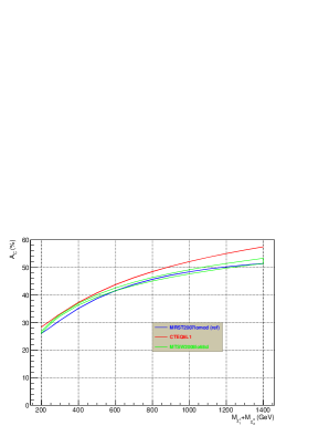
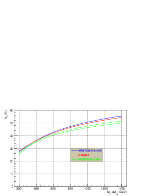
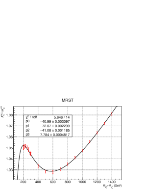
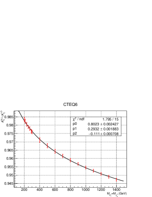
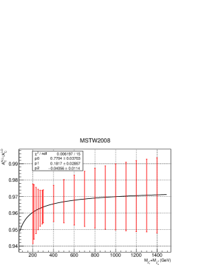
Figure 12: Comparison between the $A_{C}$ template curves. The top LHS plot compares the LO PDFs: MRST2007lomod (blue, ref. curve), CTEQ6L1 (red), MSTW2008lo68cl (green). The top RHS plot compares the NLO PDFs: MRST2004nlo (blue, ref. curve), CTEQ6.1 (red), MSTW2008nlo68cl (green). The middle and the bottom rows display the $\frac{A_{C}^{NLL}}{A_{C}^{LO}}$ fitted by the same functional forms as the $A_{C}^{LO}$ template curves.

3.2 Experimental Measurement of $A_{C}(\tilde{\chi}^{\pm}_{1}+\tilde{\chi}^{0}_{2}\to 3\ell^{\pm}+\hbox to0.0pt{\kern 2.5pt/\hss}E_{T})$

The aim of this sub-section is to repeat, in the context of the considered SUSY signal, a study similar to that of section 2.2.

We use Simplified Models to generate our signal in the two configurations shown in figure 13.

The first signal configuration, denoted S1, supposes that the lightest part of the SUSY mass spectrum is made of $\tilde{\chi}^{\pm}_{1}$, $\tilde{\chi}^{0}_{2}$, $\tilde{\ell}^{\pm}$ (i.e. $\tilde{e}^{\pm}$ or $\tilde{\mu}^{\pm}$), and $\tilde{\chi}^{0}_{1}$, in order of decreasing mass. In addition, the following decays (and their charge conjugate) are all supposed to have a braching ratio of $100\%$: $\tilde{\chi}^{\pm}_{1}\to\tilde{\ell}^{\pm}(\to\ell^{\pm}\tilde{\chi}^{0}_{1})+\nu$, $\tilde{\chi}^{0}_{2}\to\tilde{\ell}^{\pm}(\to\ell^{\pm}\tilde{\chi}^{0}_{1})+\ell^{\mp}$. In practice, within the MSSM, very large braching ratios for these decays are guaranteed by the envisaged mass hierarchy.

The second signal configuration, denoted S2, supposes that the lightest part of the SUSY mass spectrum is made of $\tilde{\chi}^{\pm}_{1}$, $\tilde{\chi}^{0}_{2}$, and $\tilde{\chi}^{0}_{1}$, in order of decreasing mass. The charged sleptons are supposed to be much heavier. In addition, the following SUSY decays are all supposed to have a braching ratio of $100\%$: $\tilde{\chi}^{\pm}_{1}\to W^{\pm}(\to\ell^{\pm}\nu)+\tilde{\chi}^{0}_{1}$, $\tilde{\chi}^{0}_{2}\to Z^{0}(\to\ell^{\pm}\ell^{\mp})+\tilde{\chi}^{0}_{1}$. In practice, within the MSSM, these braching ratios not only depend on the envisaged mass hierarchy, but also on the fields composition of the $\tilde{\chi}^{0}_{2}$, the $\tilde{\chi}^{\pm}_{1}$, and the $\tilde{\chi}^{0}_{1}$. Regarding the SM leptonic decays of the $W^{\pm}$ and the $Z^{0}$ gauge bosons, we used their actual SM branching ratios. This will have the obvious consequence of a much smaller event yield for the S2 signals compared to the S1 signals of same mass.

The hypotheses common to configurations S1 and S2 are that the lightest SUSY particle (LSP) is the $\tilde{\chi}^{0}_{1}$, and that the $\tilde{\chi}^{0}_{2}$ and the $\tilde{\chi}^{\pm}_{1}$ are mass degenerate.

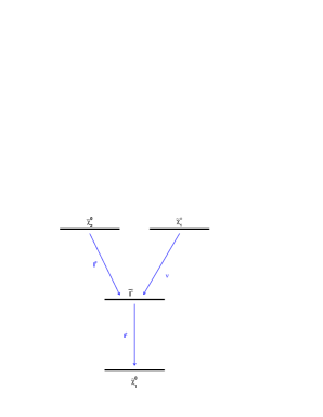
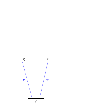
Figure 13: The sketch of the Simplified Models used to generate the signal samples: the S1 signal (LHS) has a $\tilde{\ell}^{\pm}$ NLSP whereas for the S2 signal (RHS) the mass degenerate $\tilde{\chi}^{\pm}_{1}$ and $\tilde{\chi}^{0}_{2}$ are the NLSPs. Both signals share the $\tilde{\chi}^{0}_{1}$ as the LSP.

3.2.1 Monte Carlo Generation

We generate a new set of MC samples. We report here only the MC parameters that are different from those used in sub-section 2.2.1. We use the following LO generator: Herwig++ v2.5.2 for the SUSY signal and for most of the background processes.

The other background processes: $W^{+}+W^{-}+W^{\pm}$, $W^{+}+W^{-}+\gamma^{*}/Z$, $W^{\pm}+\gamma^{*}/Z+\gamma^{*}/Z$ $\gamma^{*}/Z+\gamma^{*}/Z+\gamma^{*}/Z$, $W^{\pm}+1c+0Lp$, $W^{\pm}+1c+1Lp$, $W^{\pm}+c\bar{c}+0Lp$, $W^{\pm}+b\bar{b}+0Lp$, $W^{\pm}+t\bar{t}+0Lp$ are generated using Alpgen v2.14 at the parton level. Those samples are passed on to Pythia v8.170 for the parton showering, the fragmentation of the colored particles, the modelling of the underlying event and the decay of the unstable particles.

For the $W^{\pm}+HF$ process, and the VVV processes in Alpgen the only decay mode generated is $\gamma^{*}/Z(\to f\bar{f})$ where $f=\ell^{\pm},\tau^{\pm},\nu,q$ and $75<M(f\bar{f})<125$ GeV, whereas for the $W^{\pm}(\to e^{\pm}\nu_{e}/\mu^{\pm}\nu_{\mu}/\tau^{\pm}\nu_{\tau})$ process no mass cuts are applied.

For the $W+HF$ processes, the renormalization scale is set to

$$\mu_{R}=\mu_{F}=\sqrt{M^{2}(W)+\sum^{N^{FS}_{p}}_{i=1}M^{2}_{T}(i)}$$

where the i index runs over the number of FS partons $N^{FS}_{p}$, and where $M^{2}_{T}=M^{2}+p^{2}_{T}$.

In particular for the signal samples, we test distinct mass hypotheses in different configurations.

For the S1 signal, we vary $M_{\tilde{\chi}^{0}_{2}}$ in the range [100,700] GeV by steps of 100 GeV, and we set $M_{\tilde{\chi}^{0}_{1}}=M_{\tilde{\chi}^{0}_{2}}/2$ and $M_{\tilde{\ell}^{\pm}}=[M_{\tilde{\chi}^{0}_{2}}+M_{\tilde{\chi}^{\pm}_{1}}]/2$.

For the S2 signal, we produce a single "S2a" sample, i.e. with $M_{\tilde{\chi}^{0}_{2}}-M_{\tilde{\chi}^{0}_{1}}<M_{Z}$, for which we set $M_{\tilde{\chi}^{0}_{2}}=100$ GeV, $M_{\tilde{\chi}^{0}_{1}}=50$ GeV. This enables to explore the case where the $\tilde{\chi}^{\pm}_{1}$ and the $\tilde{\chi}^{0}_{2}$ decay through a $W^{\pm}$ and through a $Z$ that are both off-shell. For the other S2 samples, denoted "S2b" and described in the following paragraph, both the $W^{\pm}$ and the $Z$ bosons are on-shell. In addition, we vary $M_{\tilde{\chi}^{0}_{2}}$ in the range [200,700] GeV by steps of 100 GeV, setting $M_{\tilde{\chi}^{0}_{1}}=M_{\tilde{\chi}^{0}_{2}}/2$. We also vary $M_{\tilde{\chi}^{0}_{2}}$ in the range [105,145] GeV by steps of 10 GeV with a fixed value of $M_{\tilde{\chi}^{0}_{1}}=13.8$ GeV. And finally, we added two samples: $[M_{\tilde{\chi}^{0}_{2}},M_{\tilde{\chi}^{0}_{1}}]=$ [150,50] GeV and [250,125] GeV.

3.2.2 Analysis of the $\tilde{\chi}^{\pm}_{1}\tilde{\chi}^{0}_{2}\to 3\ell^{\pm}+\hbox to0.0pt{\kern 2.5pt/\hss}E_{T}$ Process

We considered only the electron and the muon channels. For these analyses we set the integrated luminosity to $\int{\cal L}dt=20\ \ fb^{-1}$.

1). Event Selection in the Trilepton Channel

A first set of requirements related to the leptons are applied for the event selection as mentioned hereafter:

1. $N(\ell^{\pm})\geq 3$

2. Electron candidates:

   1. $|\eta(e^{\pm})|<1.37\ or\ 1.53<|\eta(e^{\pm})|<2.47$

   2. $p_{T}(e^{\pm})>10$ GeV

3. Muon candidates:

   1. $|\eta(\mu^{\pm})|<2.4$

   2. $p_{T}(\mu^{\pm})>10$ GeV

4. $p_{T}(\ell^{\pm}_{1})>20$ GeV

5. $p_{T}(\ell^{\pm}_{2})>10$ GeV

6. $p_{T}(\ell^{\pm}_{3})>10$ GeV

7. Tracker Isolation: reject events with additional tracks of $p_{T}>2$ GeV within a cone of $\Delta R=0.5$ around the direction of the $\ell^{\pm}$ track

8. Calorimeter Isolation: ratio of the scalar sum of $E_{T}$ deposits in the calorimeter within a cone of $\Delta R=0.5$ around the direction of the $\ell^{\pm}$, to the $p_{T}(\ell^{\pm})$ must be less than 1.2 for $e^{\pm}$ and less than 0.25 for $\mu^{\pm}$

9. $\hbox to0.0pt{\kern 2.5pt/\hss}E_{T}>35\rm\ GeV$

10. $M_{T2}>75$ GeV

The latter cut is applied on the so-called "stransverse mass": $M_{T2}$. We used a boost-corrected calculation of this variable as described in Polesello:2009rn and implemented in MCTLib Tovey:MCTLib .

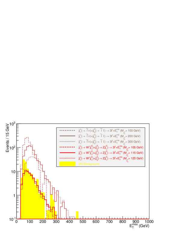
Figure 14: Distribution of the $\hbox to0.0pt{\kern 2.5pt/\hss}E_{T}$ after the event selection. The background, the S1, and the S2 signals are the filled yellow, the hollow brown, and the hollow red histograms, respectively.

$Process$	$\epsilon$	$N_{exp}$	$Z_{N}$	$A_{C}^{Exp}\pm\delta A_{C}^{Stat}$
	($\%$)	(Evts)		($\%$)
S1 Signal
$[M_{\tilde{\chi}^{0}_{2}},M_{\tilde{\ell}^{\pm}},M_{\tilde{\chi}^{0}_{1}}]$  GeV
$[100,75,50]$	$0.45\pm 0.01$	1097.43	31.70	$(7.70\pm 0.27)$
$[200,150,100]$	$4.39\pm 0.02$	702.98	23.86	$(16.06\pm 0.20)$
$[300,225,150]$	$11.41\pm 0.03$	319.48	13.79	$(21.30\pm 0.17)$
$[400,300,200]$	$16.15\pm 0.04$	113.02	6.04	$(24.40\pm 0.18)$
$[500,375,250]$	$18.98\pm 0.04$	37.96	2.25	$(27.21\pm 0.16)$
$[600,450,300]$	$21.01\pm 0.04$	12.60	0.74	$(27.20\pm 0.14)$
$[700,525,350]$	$22.66\pm 0.04$	4.53	0.23	$(29.06\pm 0.15)$
S2 Signal
$[M_{\tilde{\chi}^{0}_{2}},M_{\tilde{\chi}^{0}_{1}}]$  GeV
$[100,50]$	$9.33\pm 0.18$	0.14	-0.06	$(7.62\pm 0.38)$
$[105,13.8]$	$2.10\pm 0.01$	61.75	3.55	$(7.84\pm 0.23)$
$[115,13.8]$	$3.17\pm 0.02$	65.46	3.74	$(7.73\pm 0.21)$
$[125,13.8]$	$3.85\pm 0.02$	57.49	3.32	$(9.34\pm 0.21)$
$[135,13.8]$	$4.95\pm 0.02$	54.84	3.18	$(10.43\pm 0.17)$
$[145,13.8]$	$5.85\pm 0.02$	49.05	2.87	$(11.50\pm 0.19)$
$[150,50]$	$3.90\pm 0.02$	28.65	1.71	$(12.06\pm 0.19)$
$[200,100]$	$4.59\pm 0.02$	10.70	0.62	$(16.66\pm 0.20)$
$[250,125]$	$8.53\pm 0.03$	7.79	0.44	$(18.28\pm 0.18)$
$[300,150]$	$12.42\pm 0.03$	5.06	0.26	$(20.98\pm 0.18)$
$[400,200]$	$17.67\pm 0.04$	1.80	0.05	$(24.11\pm 0.17)$
$[500,250]$	$20.09\pm 0.04$	0.58	-0.03	$(27.51\pm 0.16)$
$[600,300]$	$21.70\pm 0.04$	0.19	-0.06	$(27.25\pm 0.18)$
$[700,350]$	$22.17\pm 0.04$	0.06	-0.07	$(27.91\pm 0.17)$
Background	-	109.51	-	$(28.04\pm 0.20)$
$W^{\pm}(\to e^{\pm}\nu_{e}/\mu^{\pm}\nu_{\mu}/\tau^{\pm}\nu_{\tau}/q\bar{q^{{}^{\prime}}})+LF$	$0.00\pm 0.00$	0.00	-	-
$W^{\pm}(\to e^{\pm}\nu_{e}/\mu^{\pm}\nu_{\mu}/\tau^{\pm}\nu_{\tau})+HF$	$0.082\pm 0.004$	0.96	-	$(36.93\pm 1.76)$
$t\bar{t}$	$0.00\pm 0.00$	0.00	-	-
$t+b,\ t+q(+b)$	$0.00\pm 0.00$	0.00	-	-
$W+W,\ W+\gamma^{*}/Z,\ \gamma^{*}/Z+\gamma^{*}/Z$	$0.283\pm 0.002$	106.78	-	$(26.95\pm 0.25)$
$W^{+}+W^{-}+W^{\pm},\ W^{+}+W^{-}+\gamma^{*}/Z,$	$0.576\pm 0.004$	1.77	-	$(29.84\pm 0.34)$
$W^{\pm}+\gamma^{*}/Z+\gamma^{*}/Z,\ \gamma^{*}/Z+\gamma^{*}/Z+\gamma^{*}/Z$			-
$\gamma+\gamma,\ \gamma+jets,\ \gamma+W^{\pm},\ \gamma+Z$	$0.00\pm 0.00$	0.00	-	-
$\gamma^{*}/Z+LF$	$0.00\pm 0.00$	0.00	-	-
$\gamma^{*}/Z+HF$	$0.00\pm 0.00$	0.00	-	-
QCD HF	$0.00\pm 0.00$	0.00	-	-
QCD LF	$0.00\pm 0.00$	0.00	-	-

Table 23: Event selection efficiencies, event yields, signal significances and charge asymmetries for the $p+p\to\tilde{\chi}^{\pm}_{1}\tilde{\chi}^{0}_{2}\to 3\ell^{\pm}+\hbox to0.0pt{\kern 2.5pt/\hss}E_{T}$ analysis.

$Process$	$\alpha^{Exp}\pm\delta\alpha^{Stat}$	$Z_{N}$	$A_{C}^{Meas.}$	$\delta A_{C}^{Tot.}$	$\delta A_{C}^{Meas.Fit}$
		($\sigma$)	($\%$)	($\%$)	($\%$)
S1 Signal
$[M_{\tilde{\chi}^{0}_{2}},M_{\tilde{\ell}^{\pm}},M_{\tilde{\chi}^{0}_{1}}]$  GeV
$[100,75,50]$	$(9.98\pm 0.26)\times 10^{-2}$	31.70	7.70	0.83	0.74
$[200,150,100]$	$(15.58\pm 0.36)\times 10^{-2}$	23.86	16.06	0.85	0.44
$[300,225,150]$	$(34.28\pm 0.79)\times 10^{-2}$	13.79	21.30	0.96	0.48
$[400,300,200]$	$(96.89\pm 2.22)\times 10^{-2}$	6.04	24.40	1.29	0.58
$[500,375,250]$	$(288.49\pm 6.61)\times 10^{-2}$	2.25	27.21	1.75	0.69
$[600,450,300]$	$(869.13\pm 19.89)\times 10^{-2}$	0.74	27.20	1.97	0.77
$[700,525,350]$	$(241.74\pm 5.55)\times 10^{-1}$	0.23	29.06	2.02	0.85
S2 Signal
$[M_{\tilde{\chi}^{0}_{2}},M_{\tilde{\chi}^{0}_{1}}]$  GeV
$[100,50]$	$(78.22\pm 6989.64)\times 10^{1}$	-0.06	7.62	0.88	0.59
$[105,13.8]$	$(177.34\pm 4.21)\times 10^{-2}$	3.55	7.85	1.58	0.56
$[115,13.8]$	$(167.29\pm 3.91)\times 10^{-2}$	3.74	7.73	1.55	0.52
$[125,13.8]$	$(190.49\pm 4.44)\times 10^{-2}$	3.32	9.34	1.60	0.49
$[135,13.8]$	$(199.69\pm 4.61)\times 10^{-2}$	3.18	10.43	1.62	0.46
$[145,13.8]$	$(223.26\pm 5.16)\times 10^{-2}$	2.87	11.50	1.67	0.45
$[150,50]$	$(382.23\pm 8.90)\times 10^{-2}$	1.71	12.06	1.85	0.44
$[200,100]$	$(102.35\pm 2.34)\times 10^{-1}$	0.62	16.66	2.00	0.46
$[250,125]$	$(140.58\pm 3.23)\times 10^{-1}$	0.44	18.28	2.01	0.52
$[300,150]$	$(216.42\pm 4.96)\times 10^{-1}$	0.26	20.98	2.02	0.60
$[400,200]$	$(608.39\pm 13.89)\times 10^{-1}$	0.05	24.11	2.03	0.74
$[500,250]$	$(18.88\pm 0.43)\times 10^{-5}$	-0.03	27.51	2.03	0.86
$[600,300]$	$(57.64\pm 1.32)\times 10^{-5}$	-0.06	27.25	2.03	0.96
$[700,350]$	$(182.52\pm 4.17)\times 10^{-5}$	-0.07	27.91	2.03	1.04

Table 24: Noise to signal ratio, signal statistical significance, and expected and measured integral charge asymmetries for the S1 and S2 signal samples for the $p+p\to\tilde{\chi}^{\pm}_{1}\tilde{\chi}^{0}_{2}\to 3\ell^{\pm}+\hbox to0.0pt{\kern 2.5pt/\hss}E_{T}$ analysis.

The event selection efficiencies, event yields, signal significances and the expected integral charge asymmetries are reported in table 23. Figure 14 displays the $\hbox to0.0pt{\kern 2.5pt/\hss}E_{T}$ distribution after the event selection.

We note that the S1 signal significance exceeds $5\sigma$ for $M_{\tilde{\chi}^{0}_{2}}=M_{\tilde{\chi}^{\pm}_{1}}$ in the [100,400] GeV interval, whereas the S2 signal significance reaches only the $3\sigma$ for 100 $<M_{\tilde{\chi}^{0}_{2}}=M_{\tilde{\chi}^{\pm}_{1}}<$ 150 GeV.

In this simple version of the analysis, we keep the same event selection for both teh S1 and the S2 signals. Therefore these signals samples share the same residual background as well as the same bias from the event selection. In these conditions, we could use a common $A_{C}$ template curve for both of them. However, because we choose many overlapping masses between these two signal samples, we split them into two seperate sets of experimental $A_{C}$ template curves. The S1 $A_{C}$ template curve, that include the propagation of the realistic experimental uncertainties into each term of equation 14, are displayed in figure 15, the S2 ones are displayed in figure 16. And the final signal template curves for which the uncertainties account for the correlations between the parameters used to fit the $A_{C}^{Meas}$ template curves are shown in figure 17, on the LHS for S1 and on the RHS for S2.

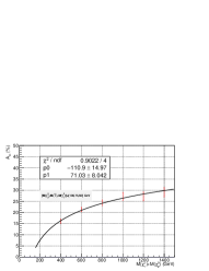
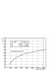
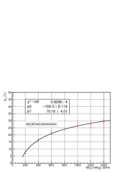
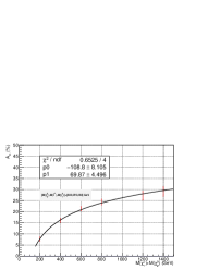
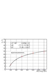
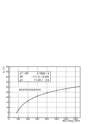
Figure 15: Experimental $A_{C}$ template curves for the S1 signal samples, as they are listed, in table 23 from the top to the bottom rows. Here, they appear ordered by increasing $\tilde{\chi}^{0}_{2}$ mass, from the top to the bottom row and from left to right.

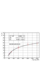
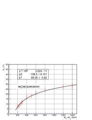
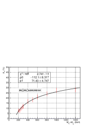
Figure 16: Experimental $A_{C}$ template curves for the S2 signal samples, as they are listed, in table 23 from the top to the bottom rows. Here, they appear ordered by increasing $\tilde{\chi}^{0}_{2}$ mass, from the top to the bottom row and from left to right.

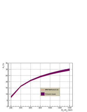
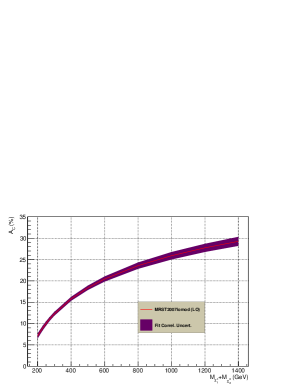
Figure 17: Fitted $A_{C}$ template curves for the S1 (LHS) and the S2 (RHS) signal samples. The uncertainty accounts for the correlations between the parameters used to fit the $A_{C}^{Meas}$ template curves.

3.3 Indirect Determination of $M_{\tilde{\chi}^{\pm}_{1}}+M_{\tilde{\chi}^{0}_{2}}$

3.3.1 Experimental Result for the S1 Signal

Using the S1 signal experimental $A_{C}$ template curves of figure 15, we can get the central values and the uncertainties of the indirectly measured $M_{\tilde{\chi}^{\pm}_{1}}+M_{\tilde{\chi}^{0}_{2}}$ for each input mass as reported in table 25.

$M_{\tilde{\chi}^{\pm}_{1}}+M_{\tilde{\chi}^{0}_{2}}$	$A_{C}^{Meas.}\pm\delta A_{C}^{Meas.Fit}$	$M_{\tilde{\chi}^{\pm}_{1}}+M_{\tilde{\chi}^{0}_{2}}$
Input Mass (GeV)	($\%$)	Measured Mass (GeV)
200.	$7.70\pm 0.74$	$200.37^{+11.51}_{-10.78}$
400.	$16.06\pm 0.44$	$390.18^{+14.83}_{-14.21}$
600.	$21.30\pm 0.48$	$617.94^{+27.70}_{-26.34}$
800.	$24.40\pm 0.58$	$824.61^{+46.98}_{-44.09}$
1000.	$27.21\pm 0.69$	$1083.15^{+76.95}_{-71.18}$
1200.	$27.20\pm 0.77$	$1082.08^{+86.18}_{-78.99}$
1400.	$29.06\pm 0.85$	$1304.01^{+118.38}_{-107.31}$

Table 25: Measured $A_{C}(S)$ of the S1 signal samples with their full experimental uncertainty. Indirect mass measurement and their full experimental uncertainty as a function of the signal sample.

This enables us to perform a closure test of our method on the S1 signal sample as displayed at the top of figure 18, where we can fit of the input versus the measured $M_{\tilde{\chi}^{\pm}_{1}}+M_{\tilde{\chi}^{0}_{2}}$ by a linear function.

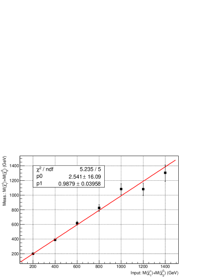
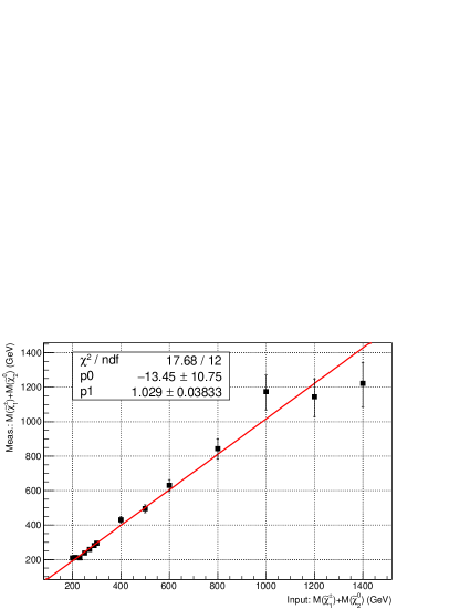
Figure 18: Closure test of the indirect measurement of $M_{\tilde{\chi}^{\pm}_{1}}+M_{\tilde{\chi}^{0}_{2}}$ for the S1 (top) and S2 (bottom) signal samples with only experimental uncertainties.

This fit indicates, given the uncertainties, that the indirect measurement is:

$$\begin{cases}\rm linear:\ the\ slope\ of\ the\ fit\ function\ is\ compatible\ with\ 1\\ \rm unbiased:\ the\ y-intercept\ of\ the\ fit\ function\ is\ compatible\ with\ 0\end{cases}$$ (42)

Further elementary checks, forcing the parameters of the fit functions, tend to confirm these indications, as presented in table 26.

Forced Parameter	Fit	Fit	Fit
	$\chi^{2}/Ndof$	Y-Intercept	Slope
Slope	5.328/6	$-1.67\pm 8.26$	$1.0\pm 0.0$
Y-Intercept	5.260/6	$0.0\pm 0.0$	$0.9933\pm 0.0203$

Table 26: Closure tests with a forced fit parameter for the S1 signal samples.

3.3.2 Experimental Result for the S2 Signal

As in the previous sub-section, using the S2 signal $A_{C}$ template curves 16, we can get the results reported in table 27. The closure test on the S2 signal samples is displayed at the bottom of figure 18.

$M_{\tilde{\chi}^{\pm}_{1}}+M_{\tilde{\chi}^{0}_{2}}$	$A_{C}^{Meas.}\pm\delta A_{C}^{Meas.Fit}$	$M_{\tilde{\chi}^{\pm}_{1}}+M_{\tilde{\chi}^{0}_{2}}$
Input Mass (GeV)	($\%$)	Measured Mass (GeV)
200.	$7.62\pm 0.59$	$208.34^{+9.51}_{-9.01}$
210.	$7.85\pm 0.56$	$211.99^{+9.20}_{-8.75}$
230.	$7.73\pm 0.52$	$210.08^{+8.43}_{-8.05}$
250.	$9.34\pm 0.49$	$237.72^{+9.01}_{-8.97}$
270.	$10.43\pm 0.46$	$258.55^{+9.52}_{-9.13}$
290.	$11.50\pm 0.45$	$281.34^{+10.29}_{-9.86}$
300.	$12.06\pm 0.44$	$294.21^{+10.60}_{-10.17}$
400.	$16.66\pm 0.46$	$430.69^{+17.35}_{-16.57}$
500.	$18.28\pm 0.52$	$495.51^{+23.17}_{-21.97}$
600.	$20.98\pm 0.60$	$630.50^{+35.51}_{-33.34}$
800.	$24.11\pm 0.74$	$843.48^{+61.79}_{-57.00}$
1000.	$27.51\pm 0.86$	$1174.45^{+105.82}_{-95.96}$
1200.	$27.25\pm 0.96$	$1144.45^{+115.34}_{-103.44}$
1400.	$27.91\pm 1.04$	$1222.38^{+135.40}_{-120.22}$

Table 27: Measured $A_{C}(S)$ of the S2 signal samples with their full experimental uncertainty. Indirect mass measurement and their full experimental uncertainty as a function of the signal sample.

Here again the fit indicates, within the uncertainties, that the indirect mass measurement is linear and unbiased. The checks, forcing the parameters of the fit functions, tend to confirm these indications, as presented in table 28.

Forced Parameter	Fit	Fit	Fit
	$\chi^{2}/Ndof$	Y-Intercept	Slope
Slope	18.27/13	$-5.601\pm 3.349$	$1.0\pm 0.0$
Y-Intercept	19.25/13	$0.0\pm 0.0$	$0.9838\pm 0.0120$

Table 28: Closure tests with a forced fit parameter for the S2 signal samples.

3.4 Final Result for MRST2007lomod

3.4.1 Final Result for the S1 Signal

Meas. $M_{\tilde{\chi}^{\pm}_{1}}+M_{\tilde{\chi}^{0}_{2}}$	Expt. Uncert.	Theor. Uncert.	Total Uncert.
(GeV)	(GeV)	(GeV)	(GeV)
200.37	${}^{+11.51}_{-10.78}$	${}^{+0.90}_{-0.90}$	${}^{+11.55}_{-10.82}$
390.18	${}^{+14.83}_{-14.21}$	${}^{+1.07}_{-1.12}$	${}^{+14.87}_{-14.25}$
617.94	${}^{+27.70}_{-26.34}$	${}^{+2.15}_{-2.24}$	${}^{+27.78}_{-26.44}$
824.61	${}^{+46.98}_{-44.09}$	${}^{+2.69}_{-2.70}$	${}^{+47.06}_{-44.17}$
1083.15	${}^{+76.95}_{-71.18}$	${}^{+2.13}_{-2.24}$	${}^{+76.98}_{-71.22}$
1082.08	${}^{+86.18}_{-78.99}$	${}^{+2.16}_{-2.24}$	${}^{+86.21}_{-79.02}$
1304.01	${}^{+118.38}_{-107.31}$	${}^{+5.76}_{-5.38}$	${}^{+118.52}_{-107.44}$

Table 29: Final results for the S1 samples with experimental and theoretical uncertainties.

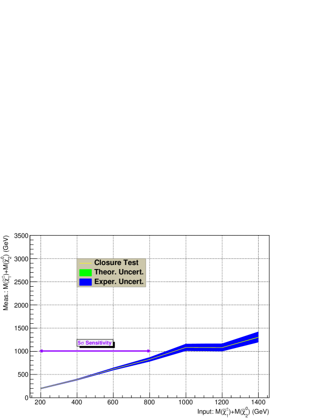
Figure 19: Closure test of the indirect measurement of $M_{\tilde{\chi}^{\pm}_{1}}+M_{\tilde{\chi}^{0}_{2}}$ for the S1 signal samples with both theoretical and experimental uncertainties. The sub-range with a signal sensitivity of $5\sigma$ is highlighted.

For the S1 sub-samples with a signal significance in excess of $5\sigma$, the indirect measurements of $M_{\tilde{\chi}^{\pm}_{1}}+M_{\tilde{\chi}^{0}_{2}}$ are performed with an overall accuracy better than $6\%$ for input masses $M_{\tilde{\chi}^{0}_{2}}=M_{\tilde{\chi}^{\pm}_{1}}$ in the [100,300] GeV interval, and better than $10\%$ for $M_{\tilde{\chi}^{0}_{2}}=M_{\tilde{\chi}^{\pm}_{1}}\geq 400$ GeV. This is reported in table 29 and displayed in figure 19.

3.4.2 Final Result for the S2 Signal

Meas. $M_{\tilde{\chi}^{\pm}_{1}}+M_{\tilde{\chi}^{0}_{2}}$	Expt. Uncert.	Theor. Uncert.	Total Uncert.
(GeV)	(GeV)	(GeV)	(GeV)
208.34	${}^{+9.51}_{-9.01}$	${}^{+0.70}_{-0.76}$	${}^{+9.54}_{-9.04}$
211.99	${}^{+9.20}_{-8.75}$	${}^{+0.66}_{-0.69}$	${}^{+9.22}_{-8.78}$
210.08	${}^{+8.43}_{-8.05}$	${}^{+0.55}_{-0.76}$	${}^{+8.45}_{-8.09}$
237.72	${}^{+9.01}_{-8.97}$	${}^{+0.61}_{-0.64}$	${}^{+9.03}_{-8.99}$
258.55	${}^{+9.52}_{-9.13}$	${}^{+0.65}_{-0.76}$	${}^{+9.54}_{-9.16}$
281.34	${}^{+10.29}_{-9.86}$	${}^{+0.77}_{-0.86}$	${}^{+10.32}_{-9.90}$
294.21	${}^{+10.60}_{-10.17}$	${}^{+0.86}_{-0.87}$	${}^{+10.63}_{-10.21}$
430.69	${}^{+17.35}_{-16.57}$	${}^{+1.34}_{-1.44}$	${}^{+17.40}_{-16.63}$
495.51	${}^{+23.17}_{-21.97}$	${}^{+1.37}_{-1.46}$	${}^{+23.21}_{-22.02}$
630.50	${}^{+35.51}_{-33.34}$	${}^{+2.12}_{-2.24}$	${}^{+35.57}_{-33.42}$
843.48	${}^{+61.79}_{-57.00}$	${}^{+2.57}_{-2.74}$	${}^{+61.84}_{-57.07}$
1174.45	${}^{+105.82}_{-95.96}$	${}^{+2.44}_{-2.47}$	${}^{+105.85}_{-95.99}$
1144.45	${}^{+115.34}_{-103.44}$	${}^{+2.40}_{-2.53}$	${}^{+115.36}_{-103.47}$
1222.38	${}^{+135.40}_{-120.22}$	${}^{+3.38}_{-3.34}$	${}^{+135.44}_{-120.27}$

Table 30: Final results for the S2 samples with experimental and theoretical uncertainties.

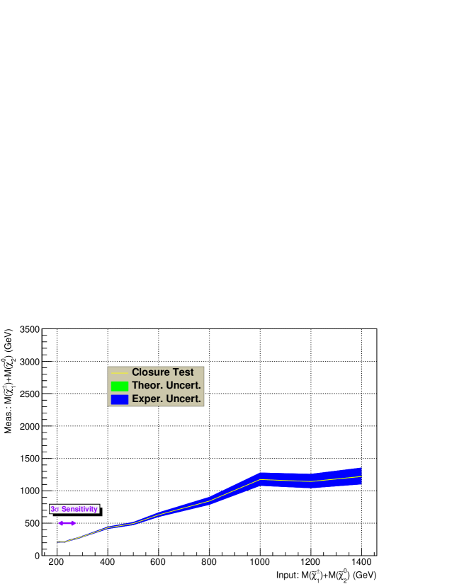
Figure 20: Closure test of the indirect measurement of $M_{\tilde{\chi}^{\pm}_{1}}+M_{\tilde{\chi}^{0}_{2}}$ for the S2 signal samples with both theoretical and experimental uncertainties. The sub-range with a signal sensitivity of $3\sigma$ is highlighted.

For the S2 sub-samples with a signal significance in excess of $3\sigma$, the indirect measurements of $M_{\tilde{\chi}^{\pm}_{1}}+M_{\tilde{\chi}^{0}_{2}}$ are performed with an overall accuracy better than $4.5\%$ for respective input masses $M_{\tilde{\chi}^{0}_{2}}=M_{\tilde{\chi}^{\pm}_{1}}$ in the [105,145] GeV interval and better than $11.1\%$ for considered masses outside this interval. This is reported in table 30 and displayed in figure 20.

3.5 Summary of the $M_{\tilde{\chi}^{\pm}_{1}}+M_{\tilde{\chi}^{0}_{2}}$ Measurements and their Accuracy

We sum up the indirect mass measurements of $M_{\tilde{\chi}^{\pm}_{1}}+M_{\tilde{\chi}^{0}_{2}}$ extracted from the integral charge asymmetry of the $\tilde{\chi}^{\pm}_{1}+\tilde{\chi}^{0}_{2}\to 3\ell^{\pm}+\hbox to0.0pt{\kern 2.5pt/\hss}E_{T}$ inclusive process within tables 31 (S1 signal) and 32 (S2 signal).

S1 Signal	Figures of Merit
Input $M_{\tilde{\chi}^{\pm}_{1}}+M_{\tilde{\chi}^{0}_{2}}$	1.	2.	3.
(GeV)	$\frac{\delta M^{Fit}_{\tiny\tilde{\chi}^{\pm}_{1}\tilde{\chi}^{0}_{2}}}{M^{Fit}_{\tiny\tilde{\chi}^{\pm}_{1}\tilde{\chi}^{0}_{2}}}$	$\frac{(M^{Fit}_{\tiny\tilde{\chi}^{\pm}_{1}\tilde{\chi}^{0}_{2}}-M^{True}_{\tiny\tilde{\chi}^{\pm}_{1}\tilde{\chi}^{0}_{2}})}{M^{True}_{\tiny\tilde{\chi}^{\pm}_{1}\tilde{\chi}^{0}_{2}}}$	$\frac{(M^{Fit}_{\tiny\tilde{\chi}^{\pm}_{1}\tilde{\chi}^{0}_{2}}-M^{True}_{\tiny\tilde{\chi}^{\pm}_{1}\tilde{\chi}^{0}_{2}})}{\delta M^{Fit}_{\tiny\tilde{\chi}^{\pm}_{1}\tilde{\chi}^{0}_{2}}}$
200.	$5.8\%$	$+0.2\%$	$+0.03\sigma$
400.	$3.8\%$	$-2.5\%$	$-0.7\sigma$
600.	$4.5\%$	$+3.0\%$	$+0.7\sigma$
800.	$5.7\%$	$+3.1\%$	$+0.5\sigma$
1000.	$7.1\%$	$+8.3\%$	$+1.1\sigma$
1200.	$8.0\%$	$-9.8\%$	$-1.4\sigma$
1400.	$9.1\%$	$-6.9\%$	$-0.8\sigma$

Table 31: Summary of the indirect mass measurements of $M_{\tilde{\chi}^{\pm}_{1}}+M_{\tilde{\chi}^{0}_{2}}$ extracted from the integral charge asymmetry of the S1 signal samples. Different figures of merit of the accuracy of these measurements are presented.

S2 Signal	Figures of Merit
Input $M_{\tilde{\chi}^{\pm}_{1}}+M_{\tilde{\chi}^{0}_{2}}$	1.	2.	3.
(GeV)	$\frac{\delta M^{Fit}_{\tiny\tilde{\chi}^{\pm}_{1}\tilde{\chi}^{0}_{2}}}{M^{Fit}_{\tiny\tilde{\chi}^{\pm}_{1}\tilde{\chi}^{0}_{2}}}$	$\frac{(M^{Fit}_{\tiny\tilde{\chi}^{\pm}_{1}\tilde{\chi}^{0}_{2}}-M^{True}_{\tiny\tilde{\chi}^{\pm}_{1}\tilde{\chi}^{0}_{2}})}{M^{True}_{\tiny\tilde{\chi}^{\pm}_{1}\tilde{\chi}^{0}_{2}}}$	$\frac{(M^{Fit}_{\tiny\tilde{\chi}^{\pm}_{1}\tilde{\chi}^{0}_{2}}-M^{True}_{\tiny\tilde{\chi}^{\pm}_{1}\tilde{\chi}^{0}_{2}})}{\delta M^{Fit}_{\tiny\tilde{\chi}^{\pm}_{1}\tilde{\chi}^{0}_{2}}}$
200.	$4.6\%$	$+4.2\%$	$+0.9\sigma$
210.	$4.4\%$	$+1.0\%$	$+0.2\sigma$
230.	$4.0\%$	$-8.7\%$	$-2.4\sigma$
250.	$3.8\%$	$-4.9\%$	$-1.4\sigma$
270.	$3.7\%$	$-4.2\%$	$-1.2\sigma$
290.	$3.7\%$	$-3.0\%$	$-0.8\sigma$
300.	$3.6\%$	$-1.9\%$	$-0.5\sigma$
400.	$4.0\%$	$+7.7\%$	$+1.8\sigma$
500.	$4.7\%$	$-0.9\%$	$-0.2\sigma$
600.	$5.6\%$	$+5.1\%$	$+0.9\sigma$
800.	$7.3\%$	$+5.4\%$	$+0.7\sigma$
1000.	$9.0\%$	$+17.5\%$	$+1.7\sigma$
1200.	$10.1\%$	$-4.6\%$	$-0.5\sigma$
1400.	$11.1\%$	$-12.7\%$	$-1.3\sigma$

Table 32: Summary of the indirect mass measurements of $M_{\tilde{\chi}^{\pm}_{1}}+M_{\tilde{\chi}^{0}_{2}}$ extracted from the integral charge asymmetry of the S2 signal samples. Different figures of merit of the accuracy of these measurements are presented.

For the S1 signal at LO, this new method enables to get an accuracy better than $6\%$ for the range with $5\sigma$ sensitivity to the signal and better than $10\%$ elsewhere. Whereas for the S2 signal at LO, we get an accuracy better than $4.5\%$ for the range with $3\sigma$ sensitivity to the signal and better than $11.2\%$ elsewhere. All these indirect measurements are statistically compatible with the total uncertainty of the method.

One should bear in mind however that these results do not account for the dominant theoretical uncertainty ($\delta(A_{C})_{PDF}$).

3.6 Comparison with Other Mass Measurement Methods

3.6.1 Dilepton Mass Edge

In this sub-section, we’ll compare the ICA (Integral Charge Asymmetry) indirect mass measurement technique with two other direct mass measurement techniques.

But before entering this topic, let us mention the issue of the combinatorics within the trilepton search topology we’ve chosen. For our signal, resolving this combinatorics consists in matching the correct dilepton to its parent $\tilde{\chi}^{0}_{2}$ whilst associating the third lepton to its parent $\tilde{\chi}^{\pm}_{1}$. The $\tilde{\chi}^{0}_{2}$ leptonic decay yields two leptons with opposite-signs (OS) and same flavours (SF). In events with mixed flavours ($e^{+}e^{-}\mu^{\pm}$ or $\mu^{+}\mu^{-}e^{\pm}$), the correct assignment is obvious: the dilepton of SF comes from the $\tilde{\chi}^{0}_{2}$ and the single lepton with the other flavour comes from the $\tilde{\chi}^{\pm}_{1}$. However in order to exploit the full signal statistics, one also needs to resolve this combinatorics in tri-electron and tri-muon events. For each of these event topology involving a single flavour, there are always two combinations of OS dileptons and one combination of same-sign (SS) dilepton. Therefore we adopt a statistical solution to lift the combinatorics. In the calculation of any physical observable, for each $3e^{\pm}$ or $3\mu^{\pm}$ event, we fill the corresponding histogram with two entries from the two OS dileptons with a weight of +1 and with one entry from the single SS dilepton with a weight of -1. This systematically subtracts from the observable histogram the wrong combination which associates a lepton from the $\tilde{\chi}^{\pm}_{1}$ decay with one of the $\tilde{\chi}^{0}_{2}$ decay.

3.6.1. a. Experimental Observable

The fact that the OS-SF dilepton coming from the second neutralino decay has an edge in its invariant mass was noted long ago in Baer:1994nr . It has been used extensively in the litterature Muanza:1996fu Muanza:1996rk Muanza:1996gha Bachacou:1999zb , including in a few reviews like Barr:2010zj and in references therein.

For the S1 signal, we have the following mass hierarchy $M_{\tilde{\chi}^{0}_{2}}=M_{\tilde{\chi}^{\pm}_{1}}>M_{\tilde{\ell}^{\pm}}>M_{\tilde{\chi}^{0}_{1}}$ and we consider $\tilde{\chi}^{0}_{2}$ and $\tilde{\chi}^{\pm}_{1}$ two-body decays proceeding through an intermediate slepton. In this case, the edge is given by:

$$M^{Max}_{\ell^{\pm}\ell^{\mp}}=M_{\tilde{\chi}^{0}_{2}}\times\sqrt{\left(1-\frac{M^{2}_{\tilde{\ell}^{\pm}}}{M^{2}_{\tilde{\chi}^{0}_{2}}}\right)\left(1-\frac{M^{2}_{\tilde{\chi}^{0}_{1}}}{M^{2}_{\tilde{\ell}^{\pm}}}\right)}$$ (43)

For the S2 signal, we have the following mass hierarchy $M_{\tilde{\chi}^{0}_{2}}=M_{\tilde{\chi}^{\pm}_{1}}>M_{\tilde{\chi}^{0}_{1}}$ and we consider $\tilde{\chi}^{0}_{2}$ and $\tilde{\chi}^{\pm}_{1}$ decays proceeding through $W^{\pm}$ and $Z$ bosons. In these cases, the edge is given by:

$$M^{Max}_{\ell^{\pm}\ell^{\mp}}=(M_{\tilde{\chi}^{0}_{2}}-M_{\tilde{\chi}^{0}_{1}})<M_{Z}$$ (44)

for a $\tilde{\chi}^{0}_{2}$ three-body decay proceeding through an off-shell $Z^{*}$ (S2a), and by

$$M^{Max}_{\ell^{\pm}\ell^{\mp}}=(M_{\tilde{\chi}^{0}_{2}}-M_{\tilde{\chi}^{0}_{1}})\geq M_{Z}$$ (45)

for a $\tilde{\chi}^{0}_{2}$ two-body decay proceeding through an on-shell $Z$ (S2b).

In light of these formulae, we see that the mass reconstruction capabilities of this method that we’ll call DileME, for "Dilepton Mass Edge", regard exclusively the reconsctruction of mass differences.

The main systematic uncertainties of the DileME method come from the lepton energy scales. These are known to a $0.05\%$ accuracy in the ATLAS experiment at the LHC Run1, both for the electrons Aad:2014nim and the muons Aad:2014rra . Since the dilepton invariant mass is:

$$M^{2}_{\ell^{\pm}_{1}\ell^{\mp}_{2}}=2E_{\ell^{\pm}_{1}}E_{\ell^{\mp}_{2}}(1-cos\alpha_{1,2})$$ (46)

The index with values 1 or 2 refers to either of the two OS-SF leptons from the $\tilde{\chi}^{0}_{2}$ decay, and $\alpha_{1,2}$ is the angle in space between their flight directions. Neglecting the uncertainty on the angle, the relative uncertainty on $M_{\ell^{\pm}\ell^{\mp}}$ writes:

$$\frac{\delta M_{\ell^{\pm}\ell^{\mp}}}{M_{\ell^{\pm}\ell^{\mp}}}=\frac{\delta E_{\ell^{\pm}}}{E_{\ell^{\pm}}}$$ (47)

3.6.1. b. Theoretical Shape

For unpolarized $\tilde{\chi}^{0}_{2}$ and for their two-body decays, the theoretical shape of the dilepton invariant mass is known Barr:2004ze to be:

$$\frac{1}{\Gamma}\frac{d\Gamma}{dM_{\ell^{\pm}\ell^{\mp}}}=2M_{\ell^{\pm}\ell^{\mp}}$$ (48)

As seen in subsection 3.2.2, the main background process in the $\tilde{\chi}^{\pm}_{1}+\tilde{\chi}^{0}_{2}\to 3\ell^{\pm}+\hbox to0.0pt{\kern 2.5pt/\hss}E_{T}$ analysis is the $W^{\pm}+\gamma^{*}/Z^{0}\to 3\ell^{\pm}+\hbox to0.0pt{\kern 2.5pt/\hss}E_{T}$ process, which constitutes an irreducible background. The OS-SF dilepton coming from the $\gamma^{*}/Z^{0}$ decay forms a peak centered around $M_{Z}$. Therefore, we model the invariant mass distribution of events surviving our selection using the following 6-parameters functional form:

$$M^{Fit}(x)=\frac{C_{3}}{2\pi}\times\frac{C_{5}}{(x-C_{4})^{2}+\frac{C_{5}^{2}}{4}}+\begin{cases}2C_{1}\times\frac{x}{C^{2}_{0}},&\ for\ x<C_{0};\ and\\ 0,&\ for\ x>C_{0}\end{cases}$$ (49)

In order to account for the detector finite resolution, we convoluted the previous functional form with a gaussian distribution centered on zero and with an RMS set to $C_{2}$. The other parameters represent:

• $C_{0}$: $M^{Max}_{\ell^{\pm}\ell^{\mp}}$, i.e. the position of the dilepton edge;

• $C_{1}$: $N^{Exp}_{S}$, i.e. the number of expected signal events under the triangle;

• $C_{3}$: $N^{Exp}_{B}$, i.e. the number of expected background events under the Z peak;

• $C_{4}$: $M_{Z}$, i.e. the position of the Z peak; and,

• $C_{5}$: $\Gamma_{Z}$, i.e. the width of the Z peak.

For the S2b signal samples, we expect $N^{Exp}_{S}+N^{Exp}_{B}$ events under the Z peak.

After a few trials we find it is sufficient to use the same triangle distribution to describe both the two-body and the three-body $\tilde{\chi}^{0}_{2}$ decay in these fits.

The results of these fits are presented in tables 33 and 34. The plots 21 and 22 illustrate a few of these fits. Obviously the highest $M_{\tilde{\chi}^{0}_{2}}$ mass hypotheses unable any measurement of the dilepton invariant mass edge because of their unsufficient signal-to-noise ratio. This situation is met for $M_{\tilde{\chi}^{0}_{2}}\geq$ 700 GeV for the S1 samples and $M_{\tilde{\chi}^{0}_{2}}\geq$ 400 GeV for the S2 samples.

Process	Theor. $M_{\ell^{+}\ell^{-}}^{Edge}$	Meas. $M_{\ell^{+}\ell^{-}}^{Edge}$	Fit $\chi^{2}/N_{dof}$
	(GeV)	(GeV)
Signal S1
$[M_{\tilde{\chi}^{0}_{2}},M_{\tilde{\ell}^{\pm}},M_{\tilde{\chi}^{0}_{1}}]$  GeV
$[100,75,50]$	49.301	$49.000\pm 0.000(stat)\pm 0.025(syst)$	1.010
$[200,150,100]$	98.601	$97.000\pm 0.000(stat)\pm 0.049(syst)$	0.263
$[300,225,150]$	147.902	$147.8\pm 4.8(stat)\pm 0.074(syst)$	0.120
$[400,300,200]$	197.203	$196.500\pm 0.000(stat)\pm 0.098(syst)$	0.067
$[500,375,250]$	246.503	$246.93\pm 0.08(stat)\pm 0.123(syst)$	0.093
$[600,450,300]$	295.804	$300.8\pm 0.7(stat)\pm 0.150(syst)$	0.097
$[700,525,350]$	345.105	–	–

Table 33: Dilepton mass edge measurements for the S1 samples.

Process	Theor. $M_{\ell^{+}\ell^{-}}^{Edge}$	Meas. $M_{\ell^{+}\ell^{-}}^{Edge}$	Fit $\chi^{2}/N_{dof}$
	(GeV)	(GeV)
Signal S2
$[M_{\tilde{\chi}^{0}_{2}},M_{\tilde{\chi}^{0}_{1}}]$  GeV
$[100,50]$	50.0	$52.35\pm 0.22(stat)\pm 0.026(syst)$	0.274
$[105,13.8]$	91.2	$91.16\pm 7.52(stat)\pm 0.046(syst)$	0.172
$[115,13.8]$	101.2	$90.28\pm 6.62(stat)\pm 0.045(syst)$	0.154
$[125,13.8]$	111.2	$88.16\pm 3.33(stat)\pm 0.040(syst)$	0.132
$[135,13.8]$	121.2	$90.13\pm 6.54(stat)\pm 0.045(syst)$	0.116
$[145,13.8]$	131.2	$88.29\pm 6.03(stat)\pm 0.044(syst)$	0.125
$[150,50]$	100.0	$99.54\pm 4.16(stat)\pm 0.050(syst)$	0.230
$[200,100]$	100.0	$91.92\pm 1.99(stat)\pm 0.046(syst)$	0.125
$[250,125]$	125.0	$91.27\pm 1.97(stat)\pm 0.046(syst)$	0.154
$[300,150]$	150.0	$91.17\pm 0.94(stat)\pm 0.046(syst)$	0.126
$[400,200]$	200.0	–	–
$[500,250]$	250.0	–	–
$[600,300]$	300.0	–	–
$[700,350]$	350.0	–	–

Table 34: Dilepton mass edge measurements for the S2 samples.

First of all we notice, that ICA and DileME methods do not give access to the same informations: $M_{\tilde{\chi}^{0}_{2}}+M_{\tilde{\chi}^{\pm}_{1}}$, versus $M_{\tilde{\chi}^{0}_{2}}-M_{\tilde{\chi}^{0}_{1}}$ or $M_{\tilde{\chi}^{0}_{2}}\times\sqrt{\left(1-\frac{M^{2}_{\tilde{\ell}^{\pm}}}{M^{2}_{\tilde{\chi}^{0}_{2}}}\right)\left(1-\frac{M^{2}_{\tilde{\chi}^{0}_{1}}}{M^{2}_{\tilde{\ell}^{\pm}}}\right)}$, respectively. We notice that the DileME method is very accurate: better than $3.5\%$ (and most often better than $1\%$) for the S1 samples, and better than $0.5\%$ for the S2a sample. However, for the S2b signal samples, it fails to extract any sensible informations about the mass difference because of the resonant mode of the $\tilde{\chi}^{0}_{2}$ decay. For the sample $(105,13.8)$ S2b sample, the correct mass difference is found by chance, whereas for the other S2b samples, the DileME method systematically provides a wrong answer: $M_{\tilde{\chi}^{0}_{2}}-M_{\tilde{\chi}^{0}_{1}}=M_{Z}$.

In regard of these observations, we conclude that the ICA and DileME methods complement very well each other.

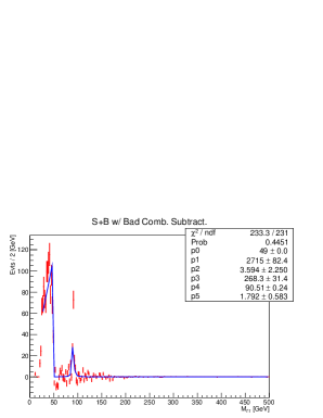
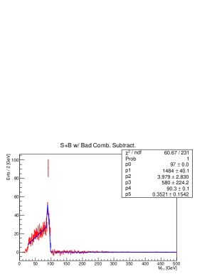
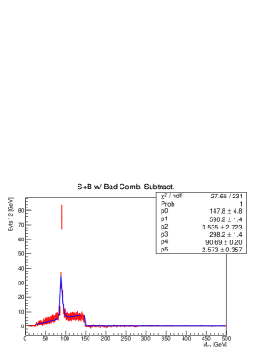
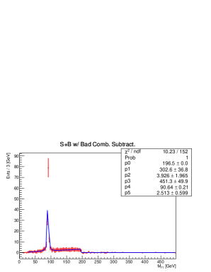
Figure 21: A few examples of DileME measurements on the S1 samples for 100 $\leq M_{\tilde{\chi}^{0}_{2}}\leq$ 400 GeV

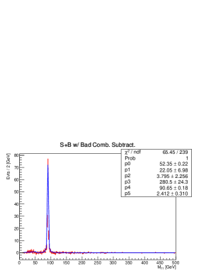
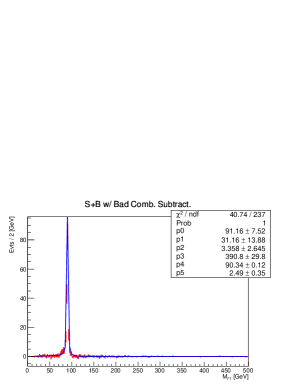
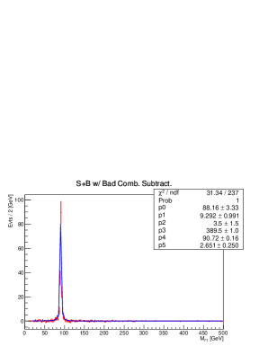
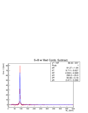
Figure 22: A few examples of DileME measurements on the S2 samples for 100 $\leq M_{\tilde{\chi}^{0}_{2}}\leq$ 250 GeV

3.6.2 Stransverse Mass End-Point

3.6.2. a. Experimental Observable

Let’s consider an event where two particles (X) and (Y) are produced. Let’s consider they both undergo decay chains, both ending up by the same invisible particle, denoted $\chi$, while emitting some visible energy in each hemispheres (A) and (B): $E^{vis_{(A)}}$ and $E^{vis_{(B)}}$. For an hypothesized mass of $\chi$, $M^{trial}_{\chi}$, the event stranverse mass $M_{T2}$ is defined as:

$$M_{T2}(vis^{(A)},vis^{(B)}|M^{trial}_{\chi})=\underset{\hbox to0.0pt{\kern 2.5pt/\hss}\vec{E}^{(A)}_{T}+\hbox to0.0pt{\kern 2.5pt/\hss}\vec{E}^{(B)}_{T}=\hbox to0.0pt{\kern 2.5pt/\hss}\vec{E}_{T}}{Min}\left\{Max[M_{T}(\vec{p}^{vis_{(A)}}_{T},\hbox to0.0pt{\kern 2.5pt/\hss}\vec{E}^{(A)}_{T});M_{T}(\vec{p}^{vis_{(B)}}_{T},\hbox to0.0pt{\kern 2.5pt/\hss}\vec{E}^{(B)}_{T})]\right\}$$ (50)

where

$$M^{2(A)}_{T}=M^{2(A)}+M^{2(\chi_{{}_{A}})}+2[E^{(A)}_{T}\cdot E^{(\chi_{{}_{A}})}_{T}-\vec{p}^{(A)}_{T}\cdot\vec{p}^{(\chi_{{}_{A}})}_{T}]$$ (51)

, and

$$E^{2}_{T}=M^{2}+p^{2}_{T}$$ (52)

The stranverse mass has two important properties. On the one hand, it’s very effective to discriminitate R-parity conserved SUSY signals from their SM background processes. On the other hand it enables to measure the mass of the parent particles (X) and (Y) and of children particle ($\chi$) and for this second purpose, we’ll denote this method MT2 in the rest of this article.

Regarding the signal and background discrimination described in section 3.2, we arbitrarily chose the following assignment:

• $\ell^{\pm}_{1}\leftrightarrow$ visible energy (A),

• $\ell^{\pm}_{2}\leftrightarrow$ visible energy (B),

• $\ell^{\pm}_{3}\leftrightarrow$ downstream additional visible particle,

where the index $i=1,2,3$ refers to the decreasing $p_{T}$ of the leptons, and we set $M^{trial}_{\chi}=0$ GeV. This choice does not accurately reflect the actual kinematics of our signal samples, but it is sufficient to provide a good and simple signal to background discrimination applicable to all of them.

On the contrary, in the current section, in order to assess the mass measurement capability of the MT2 method we have to properly assign the OS-SF dilepton to the $\tilde{\chi}^{0}_{2}$ decay, say into the visible energy (A), and the additional lepton to the $\tilde{\chi}^{\pm}_{1}$ decay into the visible energy (B). This precise assignment is done via the solution we adopted to solve the trilepton combinatorics which is presented in the preamble of the current section.

The main systematic uncertainties for the MT2 method come from the reconstruction of the different objects in our search topology. As inferred from Aad:2012twa , we consider as sources of uncertainty: the trigger, the reconstruction, the identification, the energy resolution and the isolation for both the electrons and the muons. The resulting uncertainties are $4.6\%\ (e^{\pm})$ and $1.1\%\ (\mu^{\pm})$, respectively. These changes in the electrons and muons kinematics are propagated onto a corrected missing transverse energy $\hbox to0.0pt{\kern 2.5pt/\hss}E^{Corr}_{T}$. Then, the impact of the uncertainties of the calorimeter cluster energy scale, of the jet energy scale and the jet energy resolution, and of the pile-up on the $\hbox to0.0pt{\kern 2.5pt/\hss}E_{T}$, are also summed in quadrature, amounting to an uncertainty of $0.8\%$ with which the $\hbox to0.0pt{\kern 2.5pt/\hss}E^{Corr}_{T}$ is smeared. We input the smeared $\hbox to0.0pt{\kern 2.5pt/\hss}E^{Corr}_{T}$ and the smeared lepton kinematics into the calculation of a smeared $M_{T2}^{Smear}$. Finally, the systematic uncertainty on $M_{T2}$ is taken as the absolute value of the relative difference between the nominal $M_{T2}$ and $M_{T2}^{Smear}$:

$$\frac{\delta M_{T2}}{M_{T2}}=\frac{|M_{T2}-M_{T2}^{Smear}|}{M_{T2}}.$$ (53)

This procedure is re-iterated for each value of $M^{trial}_{\chi}$, as reported in table 35.

$M^{trial}_{\chi}$ (GeV)	$\frac{\delta M_{T2}}{M_{T2}}$ ($\%$)
0.	1.86
13.8	1.80
50.	1.47
100.	1.10
125.	1.02
150.	0.97
200.	0.90
250.	0.85
300.	0.83
350.	0.81

Table 35: Systematic uncertainty on $M_{T2}$ for different $M^{trial}_{\chi}$.

3.6.2. b. Theoretical End-Points

In order to measure the end-points ($M_{T2}^{Max}$) of the $M_{T2}$ distributions we use either descending step functions or continuous but not derivable linear functions, depending on the position of this end-points with respect to the remaining background.

The positions of these end-points depend on the hypothesized value of $M^{trial}_{\chi}$ and have a kink at $M^{trial}_{\chi}=M_{\tilde{\chi}^{0}_{1}}$ Cho:2007dh . Therefore, they are described by continuous functions (yet not derivable at the kink position): one, that we’ll denote $f_{down}$ for $M^{trial}_{\chi}<M_{\tilde{\chi}^{0}_{1}}$ and another one, denoted $f_{up}$ for $M^{trial}_{\chi}>M_{\tilde{\chi}^{0}_{1}}$.

For two-body decays, the $f_{down}$ and $f_{up}$ functions are:

$$\begin{split}f^{2-body}_{down}=M^{Max}_{T2}\left(\ell^{\pm}_{(A)},\ell^{\pm}\ell^{\mp}_{(B)}|M^{trial}_{\chi}<M_{\tilde{\chi}^{0}_{1}}\right)=\left(\frac{M^{2}_{\tilde{\chi}^{0}_{2}}+M^{2}_{\tilde{\ell}^{\pm}}-M^{2}_{\tilde{\chi}^{0}_{1}}}{2M_{\tilde{\chi}^{0}_{2}}}\right)+\\ \sqrt{\left(\frac{M^{2}_{\tilde{\chi}^{0}_{2}}-M^{2}_{\tilde{\ell}^{\pm}}+M^{2}_{\tilde{\chi}^{0}_{1}}}{2M_{\tilde{\chi}^{0}_{2}}}\right)^{2}+[(M^{trial}_{\chi})^{2}-M^{2}_{\tilde{\chi}^{0}_{1}}]}\end{split}$$ (54)

and,

$$\begin{split}f^{2-body}_{up}=M^{Max}_{T2}\left(\ell^{\pm}_{(A)},\ell^{\pm}\ell^{\mp}_{(B)}|M^{trial}_{\chi}>M_{\tilde{\chi}^{0}_{1}}\right)=\frac{M_{\tilde{\chi}^{0}_{2}}}{2}\left((1-\frac{M^{2}_{\tilde{\ell}^{\pm}}}{M^{2}_{\tilde{\chi}^{0}_{2}}})+(1-\frac{M^{2}_{\tilde{\chi}^{0}_{1}}}{M^{2}_{\tilde{\ell}^{\pm}}})\right)+\\ \sqrt{\left[\frac{M_{\tilde{\chi}^{0}_{2}}}{2}\left((1-\frac{M^{2}_{\tilde{\ell}^{\pm}}}{M^{2}_{\tilde{\chi}^{0}_{2}}})-(1-\frac{M^{2}_{\tilde{\chi}^{0}_{1}}}{M^{2}_{\tilde{\ell}^{\pm}}})\right)\right]^{2}+(M^{trial}_{\chi})^{2}}\end{split}$$ (55)

Whereas, for three-body decays, the $f_{down}$ and $f_{up}$ functions are:

$$\begin{split}f^{3-body}_{down}=M^{Max}_{T2}\left(\ell^{\pm}_{(A)},\ell^{\pm}\ell^{\mp}_{(B)}|M^{trial}_{\chi}<M_{\tilde{\chi}^{0}_{1}}\right)=\left(\frac{M^{2}_{\tilde{\chi}^{0}_{2}}-M^{2}_{\tilde{\chi}^{0}_{1}}}{2M_{\tilde{\chi}^{0}_{2}}}\right)+\\ \sqrt{\left(\frac{M^{2}_{\tilde{\chi}^{0}_{2}}-M^{2}_{\tilde{\chi}^{0}_{1}}}{2M_{\tilde{\chi}^{0}_{2}}}\right)^{2}+(M^{trial}_{\chi})^{2}}\end{split}$$ (56)

and,

$$f^{3-body}_{up}=M^{Max}_{T2}\left(\ell^{\pm}_{(A)},\ell^{\pm}\ell^{\mp}_{(B)}|M^{trial}_{\chi}>M_{\tilde{\chi}^{0}_{1}}\right)=(M_{\tilde{\chi}^{0}_{2}}-M_{\tilde{\chi}^{0}_{1}})+M^{trial}_{\chi}$$ (57)

It’s important to note, that for $f^{2-body}_{down}$, small values of $M^{trial}_{\chi}$ are not always permitted. In the particular for our simplified models, we have the following relations: $M_{\tilde{\chi}^{0}_{2}}=2M_{\tilde{\chi}^{0}_{1}}$, and for the S1 samples, $M_{\tilde{\ell}^{\pm}}=\frac{3}{2}M_{\tilde{\chi}^{0}_{1}}$. Therefore we need to keep $M^{trial}_{\chi}\geq\sqrt{\frac{135}{256}}\times M_{\tilde{\chi}^{0}_{1}}$ in order for $f^{2-body}_{down}$ to be defined.

For the MT2 method, we need to perform two series of fits. We start with primary fits to the $M_{T2}$ distributions for each signal sample so as to measure their $M^{Max}_{T2}$. Then we proceed with the secondary fits for each signal sample. The latter use as inputs the different $M^{Max}_{T2}$ values obtained for each $M^{trial}_{\chi}$ hypothesis and they enable simultaneoulsy to measure the mass of the parent particle, here $M_{\tilde{\chi}^{0}_{2}}=M_{\tilde{\chi}^{\pm}_{1}}$, of the end daughter particle $M_{\tilde{\chi}^{0}_{1}}$ and, for the S1 samples, the mass of the intermediate particle, $M_{\tilde{\ell}^{\pm}}$. The 2-body functional forms are utilized to fit the S1 samples and the 3-body ones are utilized to fit the S2 samples. Note that these functional forms also provide the prior knowledge of the $M^{Max}_{T2}$ for each signal hypothesis which serve as starting points in the minimization process of the primary fits.

Here are a few important observations that justify our strategy for the primary fits:

• the $M_{T2}$ distribution of the remaining background events cluster into a Z peak which is located at $M_{Z}+M^{trial}_{\chi}$,

• the $M_{T2}$ distribution of the S2b samples also cluster into a Z peak which is located at $M_{Z}+M^{trial}_{\chi}$ and which may either be truncated or exhibit an asymmetric shoulder,

• S1 samples: without an analytical description of the full $M_{T2}$ distribution, we just fit the $M_{T2}$ falling edge.

This leads us to use similar functional forms as for the dilepton mass distributions for the primary fits, but with 8 parameters:

$$M^{Fit}(x)=\frac{C_{5}}{2\pi}\times\frac{C_{7}}{(x-C_{6})^{2}+\frac{C_{7}^{2}}{4}}+\begin{cases}C_{1}\times(x-C_{0})+C_{2},&\rm\ for\ x<C_{0};\ and\\ C_{3}\times(x-C_{0})+C_{2},&\rm\ for\ x>C_{0}\end{cases}$$ (58)

In order to account for the detector finite resolution, we convoluted the previous functional form with a gaussian distribution centered on zero and with an RMS set to $C_{4}$. The other parameters represent:

• $C_{0}$: $M^{Max}_{T2}$, i.e. the position of the $M_{T2}$ end-point;

• $C_{1}$: slope of the first line;

• $C_{2}$: height of the kink between the two lines;

• $C_{3}$: slope of the second line;

• $C_{5}$: $N^{Exp}_{B}$, i.e. the number of expected background events under the Z peak;

• $C_{6}$: $M_{Z}+M^{trial}_{\chi}$, i.e. the position of the (pseudo) Z peak; and,

• $C_{7}$: the width of the pseudo Z peak.

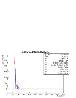
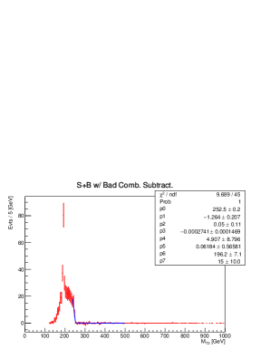
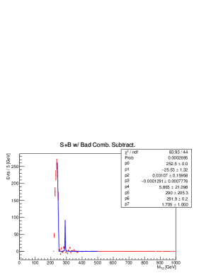
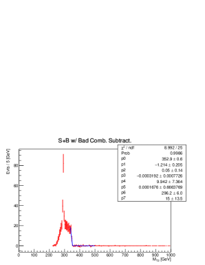
Figure 23: A few examples of $M_{T2}^{Max}$ measurements on the S1 samples. For the top and the bottom row $M_{trial}^{\chi}=$100 and 200 GeV, respectively. For the left and the right column $M_{\tilde{\chi}^{0}_{2}}=$ 100 and 300 GeV, respectively.

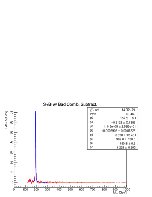
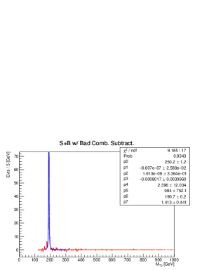
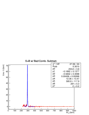
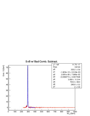
Figure 24: A few examples of $M_{T2}^{Max}$ measurements on the S2 samples. For the top and the bottom row $M_{trial}^{\chi}=$100 and 200 GeV, respectively. For the left and the right column $M_{\tilde{\chi}^{0}_{2}}=$ 100 and 300 GeV, respectively.

The results of the primary fits are presented in tables 36 to 55. Figures 23 and 24 illustrate a few of them. Again, no $M^{Max}_{T2}$ measurements on our samples are feasible when $M_{\tilde{\chi}^{0}_{2}}\geq$ 700 GeV for the S1 samples and $M_{\tilde{\chi}^{0}_{2}}\geq$ 400 GeV for the S2 samples.

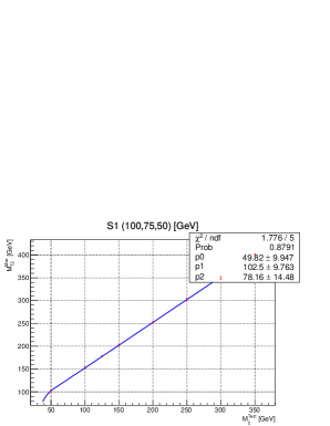
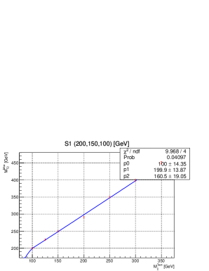
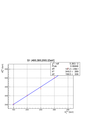
Figure 25: Examples of MT2 secondary fits to the S1 samples for $M_{\tilde{\chi}^{0}_{2}}=$100 (top left), 200 (top right), 300 (bottom left) and 400 (bottom right) GeV.

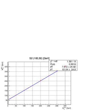
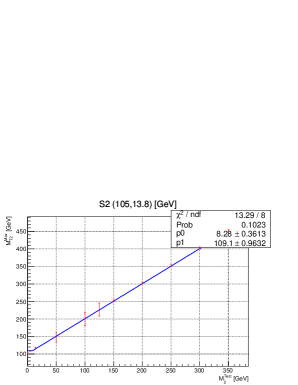
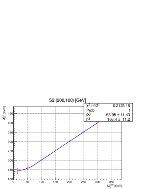
Figure 26: Examples of MT2 secondary fits to the S2 samples for $M_{\tilde{\chi}^{0}_{2}}=$100 (top left), 105 (top right), 200 (bottom left) and 300 (bottom right) GeV.

For the secondary fits, the $f_{down}$ and $f_{up}$ functional forms are directly applied onto the $(M^{Max}_{T2},M^{trial}_{\chi})$ two-dimensional plots. The results of these latter fits, that allow to extract the mass measurements, are presentend in tables 56 to 57 and a few of them are illustrated in figures 25 and 26.

Process	Theor. $M^{Max}_{T2}$	$M_{T2}$	Fit $\chi^{2}/N_{dof}$
	(GeV)	(GeV)
Signal S1
$[M_{\tilde{\chi}^{0}_{2}},M_{\tilde{\ell}^{\pm}},M_{\tilde{\chi}^{0}_{1}}]$  GeV
$[100,75,50]$	Undef.	–	–
$[200,150,100]$	Undef.	–	–
$[300,225,150]$	Undef.	–	–
$[400,300,200]$	Undef.	–	–
$[500,375,250]$	Undef.	–	–
$[600,450,300]$	Undef.	–	–
$[700,525,350]$	Undef.	–	–

Table 36: $M^{Max}_{T2}$ measurements of the S1 samples for $M^{trial}_{\chi}=0$ GeV.

Process	Theor. $M^{Max}_{T2}$	$M_{T2}$	Fit $\chi^{2}/N_{dof}$
	(GeV)	(GeV)
Signal S2
$[M_{\tilde{\chi}^{0}_{2}},M_{\tilde{\chi}^{0}_{1}}]$  GeV
$[100,50]$	75.0	$60.00\pm 18.71(stat)\pm 1.12(syst)$	1.239
$[105,13.8]$	103.2	$102.39\pm 0.42(stat)\pm 1.90(syst)$	2.637
$[115,13.8]$	113.3	$102.50\pm 0.12(stat)\pm 1.91(syst)$	0.764
$[125,13.8]$	123.5	$122.50\pm 0.03(stat)\pm 2.28(syst)$	1.006
$[135,13.8]$	133.6	$127.80\pm 2.46(stat)\pm 2.38(syst)$	0.806
$[145,13.8]$	143.7	$136.52\pm 14.31(stat)\pm 2.54(syst)$	0.719
$[150,50]$	133.3	$119.99\pm 17.12(stat)\pm 2.23(syst)$	1.205
$[200,100]$	150.0	$146.15\pm 9.99(stat)\pm 2.72(syst)$	1.210
$[250,125]$	187.5	$188.52\pm 14.57(stat)\pm 3.51(syst)$	1.245
$[300,150]$	225.0	$216.17\pm 14.50(stat)\pm 4.02(syst)$	1.007
$[400,200]$	–	–	–
$[500,250]$	–	–	–
$[600,300]$	–	–	–
$[700,350]$	–	–	–

Table 37: $M^{Max}_{T2}$ measurements of the S2 samples for $M^{trial}_{\chi}=0$ GeV.

Process	Theor. $M^{Max}_{T2}$	$M_{T2}$	Fit $\chi^{2}/N_{dof}$
	(GeV)	(GeV)
Signal S1
$[M_{\tilde{\chi}^{0}_{2}},M_{\tilde{\ell}^{\pm}},M_{\tilde{\chi}^{0}_{1}}]$  GeV
$[100,75,50]$	Undef.	–	–
$[200,150,100]$	Undef.	–	–
$[300,225,150]$	Undef.	–	–
$[400,300,200]$	Undef.	–	–
$[500,375,250]$	Undef.	–	–
$[600,450,300]$	Undef.	–	–
$[700,525,350]$	–	–	–

Table 38: $M^{Max}_{T2}$ measurements of the S1 samples for $M^{trial}_{\chi}=13.8$ GeV.

Process	Theor. $M^{Max}_{T2}$	$M_{T2}$	Fit $\chi^{2}/N_{dof}$
	(GeV)	(GeV)
Signal S2
$[M_{\tilde{\chi}^{0}_{2}},M_{\tilde{\chi}^{0}_{1}}]$  GeV
$[100,50]$	77.5	$67.49\pm 0.05(stat)\pm 1.21(syst)$	0.976
$[105,13.8]$	105.0	$117.50\pm 0.07(stat)\pm 2.11(syst)$	1.423
$[115,13.8]$	115.0	$117.50\pm 0.24(stat)\pm 2.11(syst)$	1.993
$[125,13.8]$	125.0	$117.50\pm 0.22(stat)\pm 2.11(syst)$	0.776
$[135,13.8]$	135.0	$128.25\pm 7.48(stat)\pm 2.31(syst)$	0.687
$[145,13.8]$	145.0	$158.99\pm 1.12(stat)\pm 2.86(syst)$	0.478
$[150,50]$	134.7	$142.67\pm 9.03(stat)\pm 2.57(syst)$	0.974
$[200,100]$	151.3	$143.74\pm 14.88(stat)\pm 2.59(syst)$	0.794
$[250,125]$	188.5	$192.72\pm 4.00(stat)\pm 3.47(syst)$	0.590
$[300,150]$	225.8	$219.64\pm 3.88(stat)\pm 3.95(syst)$	0.697
$[400,200]$	–	–	–
$[500,250]$	–	–	–
$[600,300]$	–	–	–
$[700,350]$	–	–	–

Table 39: $M^{Max}_{T2}$ measurements of the S2 samples for $M^{trial}_{\chi}=13.8$ GeV.

Process	Theor. $M^{Max}_{T2}$	$M_{T2}$	Fit $\chi^{2}/N_{dof}$
	(GeV)	(GeV)
Signal S1
$[M_{\tilde{\chi}^{0}_{2}},M_{\tilde{\ell}^{\pm}},M_{\tilde{\chi}^{0}_{1}}]$  GeV
$[100,75,50]$	100.0	$102.20\pm 0.31(stat)\pm 1.50(syst)$	2.555
$[200,150,100]$	Undef.	–	–
$[300,225,150]$	Undef.	–	–
$[400,300,200]$	Undef.	–	–
$[500,375,250]$	Undef.	–	–
$[600,450,300]$	Undef.	–	–
$[700,525,350]$	–	–	–

Table 40: $M^{Max}_{T2}$ measurements of the S1 samples for $M^{trial}_{\chi}=50$ GeV.

Process	Theor. $M^{Max}_{T2}$	$M_{T2}$	Fit $\chi^{2}/N_{dof}$
	(GeV)	(GeV)
Signal S2
$[M_{\tilde{\chi}^{0}_{2}},M_{\tilde{\chi}^{0}_{1}}]$  GeV
$[100,50]$	100.0	$102.49\pm 0.18(stat)\pm 1.51(syst)$	1.096
$[105,13.8]$	141.2	$148.26\pm 14.09(stat)\pm 2.18(syst)$	1.371
$[115,13.8]$	151.2	$152.50\pm 0.01(stat)\pm 2.24(syst)$	1.366
$[125,13.8]$	161.2	$153.14\pm 3.67(stat)\pm 2.25(syst)$	0.759
$[135,13.8]$	171.2	$152.50\pm 0.05(stat)\pm 2.24(syst)$	0.493
$[145,13.8]$	181.2	$190.26\pm 9.54(stat)\pm 2.80(syst)$	0.602
$[150,50]$	150.0	$152.50\pm 0.06(stat)\pm 2.24(syst)$	1.101
$[200,100]$	165.1	$156.85\pm 3.68(stat)\pm 2.31(syst)$	1.038
$[250,125]$	200.0	$197.50\pm 2.89(stat)\pm 2.90(syst)$	0.630
$[300,150]$	235.6	$246.67\pm 1.91(stat)\pm 3.63(syst)$	0.680
$[400,200]$	–	–	–
$[500,250]$	–	–	–
$[600,300]$	–	–	–
$[700,350]$	–	–	–

Table 41: $M^{Max}_{T2}$ measurements of the S2 samples for $M^{trial}_{\chi}=50$ GeV.

Process	Theor. $M^{Max}_{T2}$	$M_{T2}$	Fit $\chi^{2}/N_{dof}$
	(GeV)	(GeV)
Signal S1
$[M_{\tilde{\chi}^{0}_{2}},M_{\tilde{\ell}^{\pm}},M_{\tilde{\chi}^{0}_{1}}]$  GeV
$[100,75,50]$	149.8	$152.98\pm 0.15(stat)\pm 1.68(syst)$	2.436
$[200,150,100]$	200.0	$199.91\pm 0.35(stat)\pm 2.20(syst)$	0.559
$[300,225,150]$	Undef.	–	–
$[400,300,200]$	Undef.	–	–
$[500,375,250]$	Undef.	–	–
$[600,450,300]$	Undef.	–	–
$[700,525,350]$	–	–	–

Table 42: $M^{Max}_{T2}$ measurements of the S1 samples for $M^{trial}_{\chi}=100$ GeV.

Process	Theor. $M^{Max}_{T2}$	$M_{T2}$	Fit $\chi^{2}/N_{dof}$
	(GeV)	(GeV)
Signal S2
$[M_{\tilde{\chi}^{0}_{2}},M_{\tilde{\chi}^{0}_{1}}]$  GeV
$[100,50]$	150.0	$152.49\pm 0.09(stat)\pm 1.68(syst)$	0.584
$[105,13.8]$	191.2	$200.44\pm 18.86(stat)\pm 2.20(syst)$	1.052
$[115,13.8]$	201.2	$202.50\pm 0.01(stat)\pm 2.23(syst)$	1.138
$[125,13.8]$	211.2	$202.50\pm 0.13(stat)\pm 2.23(syst)$	0.565
$[135,13.8]$	221.2	$210.14\pm 4.50(stat)\pm 2.31(syst)$	0.491
$[145,13.8]$	231.2	$237.70\pm 12.79(stat)\pm 2.61(syst)$	0.558
$[150,50]$	200.0	$202.50\pm 0.10(stat)\pm 2.23(syst)$	0.799
$[200,100]$	200.0	$202.49\pm 0.01(stat)\pm 2.23(syst)$	0.673
$[250,125]$	230.8	$239.16\pm 14.75(stat)\pm 2.63(syst)$	0.574
$[300,150]$	263.0	$250.15\pm 1.24(stat)\pm 2.75(syst)$	0.540
$[400,200]$	–	–	–
$[500,250]$	–	–	–
$[600,300]$	–	–	–
$[700,350]$	–	–	–

Table 43: $M^{Max}_{T2}$ measurements of the S2 samples for $M^{trial}_{\chi}=100$ GeV.

Process	Theor. $M^{Max}_{T2}$	$M_{T2}$	Fit $\chi^{2}/N_{dof}$
	(GeV)	(GeV)
Signal S1
$[M_{\tilde{\chi}^{0}_{2}},M_{\tilde{\ell}^{\pm}},M_{\tilde{\chi}^{0}_{1}}]$  GeV
$[100,75,50]$	174.8	$177.86\pm 0.13(stat)\pm 1.81(syst)$	1.814
$[200,150,100]$	224.9	$225.28\pm 0.78(stat)\pm 2.30(syst)$	1.284
$[300,225,150]$	258.2	$277.64\pm 0.32(stat)\pm 2.83(syst)$	0.526
$[400,300,200]$	Undef.	–	–
$[500,375,250]$	Undef.	–	–
$[600,450,300]$	Undef.	–	–
$[700,525,350]$	–	–	–

Table 44: $M^{Max}_{T2}$ measurements of the S1 samples for $M^{trial}_{\chi}=125$ GeV.

Process	Theor. $M^{Max}_{T2}$	$M_{T2}$	Fit $\chi^{2}/N_{dof}$
	(GeV)	(GeV)
Signal S2
$[M_{\tilde{\chi}^{0}_{2}},M_{\tilde{\chi}^{0}_{1}}]$  GeV
$[100,50]$	175.0	$177.50\pm 0.06(stat)\pm 1.81(syst)$	0.742
$[105,13.8]$	216.2	$227.01\pm 18.62(stat)\pm 2.32(syst)$	1.296
$[115,13.8]$	226.2	$227.50\pm 0.01(stat)\pm 2.32(syst)$	1.228
$[125,13.8]$	236.2	$227.49\pm 0.03(stat)\pm 2.32(syst)$	0.493
$[135,13.8]$	246.2	$227.50\pm 0.04(stat)\pm 2.32(syst)$	0.461
$[145,13.8]$	256.2	$246.11\pm 6.54(stat)\pm 2.51(syst)$	0.566
$[150,50]$	225.0	$227.50\pm 0.005(stat)\pm 2.32(syst)$	1.167
$[200,100]$	225.0	$227.50\pm 0.02(stat)\pm 2.32(syst)$	0.965
$[250,125]$	250.0	$250.99\pm 18.17(stat)\pm 2.56(syst)$	0.586
$[300,150]$	280.7	$266.70\pm 1.93(stat)\pm 2.72(syst)$	0.566
$[400,200]$	–	–	–
$[500,250]$	–	–	–
$[600,300]$	–	–	–
$[700,350]$	–	–	–

Table 45: $M^{Max}_{T2}$ measurements of the S2 samples for $M^{trial}_{\chi}=125$ GeV.

Process	Theor. $M^{Max}_{T2}$	$M_{T2}$	Fit $\chi^{2}/N_{dof}$
	(GeV)	(GeV)
Signal S1
$[M_{\tilde{\chi}^{0}_{2}},M_{\tilde{\ell}^{\pm}},M_{\tilde{\chi}^{0}_{1}}]$  GeV
$[100,75,50]$	199.8	$202.50\pm 0.0003(stat)\pm 1.96(syst)$	1.857
$[200,150,100]$	249.8	$250.29\pm 0.37(stat)\pm 2.43(syst)$	0.623
$[300,225,150]$	300.0	$302.54\pm 0.52(stat)\pm 2.93(syst)$	0.345
$[400,300,200]$	300.0	$352.50\pm 0.01(stat)\pm 3.42(syst)$	0.239
$[500,375,250]$	Undef.	–	–
$[600,450,300]$	Undef.	–	–
$[700,525,350]$	–	–	–

Table 46: $M^{Max}_{T2}$ measurements of the S1 samples for $M^{trial}_{\chi}=150$ GeV.

Process	Theor. $M^{Max}_{T2}$	$M_{T2}$	Fit $\chi^{2}/N_{dof}$
	(GeV)	(GeV)
Signal S2
$[M_{\tilde{\chi}^{0}_{2}},M_{\tilde{\chi}^{0}_{1}}]$  GeV
$[100,50]$	200.0	$202.50\pm 0.51(stat)\pm 1.96(syst)$	0.920
$[105,13.8]$	241.2	$252.50\pm 0.003(stat)\pm 2.45(syst)$	1.684
$[115,13.8]$	251.2	$252.50\pm 0.02(stat)\pm 2.45(syst)$	1.574
$[125,13.8]$	261.2	$252.50\pm 0.02(stat)\pm 2.45(syst)$	0.716
$[135,13.8]$	271.2	$252.50\pm 0.03(stat)\pm 2.45(syst)$	0.505
$[145,13.8]$	281.2	$267.16\pm 19.58(stat)\pm 2.59(syst)$	0.600
$[150,50]$	250.0	$252.50\pm 0.003(stat)\pm 2.45(syst)$	1.552
$[200,100]$	250.0	$252.50\pm 0.07(stat)\pm 2.45(syst)$	1.372
$[250,125]$	275.0	$252.48\pm 0.09(stat)\pm 2.45(syst)$	0.701
$[300,150]$	300.0	$286.68\pm 2.41(stat)\pm 2.78(syst)$	0.645
$[400,200]$	–	–	–
$[500,250]$	–	–	–
$[600,300]$	–	–	–
$[700,350]$	–	–	–

Table 47: $M^{Max}_{T2}$ measurements of the S2 samples for $M^{trial}_{\chi}=150$ GeV.

Process	Theor. $M^{Max}_{T2}$	$M_{T2}$	Fit $\chi^{2}/N_{dof}$
	(GeV)	(GeV)
Signal S1
$[M_{\tilde{\chi}^{0}_{2}},M_{\tilde{\ell}^{\pm}},M_{\tilde{\chi}^{0}_{1}}]$  GeV
$[100,75,50]$	249.7	$252.54\pm 0.04(stat)\pm 2.27(syst)$	1.908
$[200,150,100]$	299.7	$290.92\pm 0.16(stat)\pm 2.62(syst)$	2.085
$[300,225,150]$	349.7	$352.89\pm 0.55(stat)\pm 3.18(syst)$	0.360
$[400,300,200]$	400.0	$402.50\pm 0.01(stat)\pm 3.62(syst)$	0.217
$[500,375,250]$	412.0	$432.60\pm 0.01(stat)\pm 3.89(syst)$	0.008
$[600,450,300]$	Undef.	–	–
$[700,525,350]$	–	–	–

Table 48: $M^{Max}_{T2}$ measurements of the S1 samples for $M^{trial}_{\chi}=200$ GeV.

Process	Theor. $M^{Max}_{T2}$	$M_{T2}$	Fit $\chi^{2}/N_{dof}$
	(GeV)	(GeV)
Signal S2
$[M_{\tilde{\chi}^{0}_{2}},M_{\tilde{\chi}^{0}_{1}}]$  GeV
$[100,50]$	250.0	$255.83\pm 3.81(stat)\pm 2.30(syst)$	1.128
$[105,13.8]$	291.2	$302.50\pm 0.05(stat)\pm 2.72(syst)$	1.739
$[115,13.8]$	301.2	$302.49\pm 0.18(stat)\pm 2.72(syst)$	1.733
$[125,13.8]$	311.2	$302.50\pm 0.05(stat)\pm 2.72(syst)$	0.603
$[135,13.8]$	321.2	$302.49\pm 0.05(stat)\pm 2.72(syst)$	0.642
$[145,13.8]$	331.2	$302.50\pm 0.07(stat)\pm 2.72(syst)$	0.592
$[150,50]$	300.0	$302.49\pm 0.07(stat)\pm 2.72(syst)$	1.597
$[200,100]$	300.0	$302.50\pm 0.08(stat)\pm 2.72(syst)$	1.613
$[250,125]$	325.0	$313.23\pm 3.74(stat)\pm 2.82(syst)$	0.844
$[300,150]$	350.0	$333.17\pm 0.86(stat)\pm 3.00(syst)$	0.694
$[400,200]$	–	–	–
$[500,250]$	–	–	–
$[600,300]$	–	–	–
$[700,350]$	–	–	–

Table 49: $M^{Max}_{T2}$ measurements of the S2 samples for $M^{trial}_{\chi}=200$ GeV.

Process	Theor. $M^{Max}_{T2}$	$M_{T2}$	Fit $\chi^{2}/N_{dof}$
	(GeV)	(GeV)
Signal S1
$[M_{\tilde{\chi}^{0}_{2}},M_{\tilde{\ell}^{\pm}},M_{\tilde{\chi}^{0}_{1}}]$  GeV
$[100,75,50]$	299.7	$302.51\pm 0.02(stat)\pm 2.57(syst)$	2.215
$[200,150,100]$	349.6	$350.38\pm 0.38(stat)\pm 2.98(syst)$	1.160
$[300,225,150]$	399.6	$401.39\pm 3.10(stat)\pm 3.41(syst)$	0.329
$[400,300,200]$	449.7	$441.63\pm 1.70(stat)\pm 3.75(syst)$	1.042
$[500,375,250]$	500.0	$502.50\pm 0.15(stat)\pm 4.27(syst)$	0.212
$[600,450,300]$	516.4	$556.34\pm 10.55(stat)\pm 4.73(syst)$	0.102
$[700,525,350]$	–	–	–

Table 50: $M^{Max}_{T2}$ measurements of the S1 samples for $M^{trial}_{\chi}=250$ GeV.

Process	Theor. $M^{Max}_{T2}$	$M_{T2}$	Fit $\chi^{2}/N_{dof}$
	(GeV)	(GeV)
Signal S2
$[M_{\tilde{\chi}^{0}_{2}},M_{\tilde{\chi}^{0}_{1}}]$  GeV
$[100,50]$	300.0	$305.18\pm 3.40(stat)\pm 2.59(syst)$	1.084
$[105,13.8]$	341.2	$352.49\pm 0.02(stat)\pm 3.00(syst)$	1.717
$[115,13.8]$	351.2	$352.49\pm 0.21(stat)\pm 3.00(syst)$	1.898
$[125,13.8]$	361.2	$352.50\pm 0.05(stat)\pm 3.00(syst)$	0.796
$[135,13.8]$	371.2	$352.50\pm 0.06(stat)\pm 3.00(syst)$	0.614
$[145,13.8]$	381.2	$362.14\pm 2.43(stat)\pm 3.08(syst)$	0.608
$[150,50]$	350.0	$352.50\pm 0.10(stat)\pm 3.00(syst)$	1.874
$[200,100]$	350.0	$352.50\pm 0.05(stat)\pm 3.00(syst)$	1.551
$[250,125]$	375.0	$362.70\pm 4.50(stat)\pm 3.08(syst)$	0.878
$[300,150]$	400.0	$380.55\pm 1.37(stat)\pm 3.23(syst)$	0.643
$[400,200]$	–	–	–
$[500,250]$	–	–	–
$[600,300]$	–	–	–
$[700,350]$	–	–	–

Table 51: $M^{Max}_{T2}$ measurements of the S2 samples for $M^{trial}_{\chi}=250$ GeV.

Process	Theor. $M^{Max}_{T2}$	$M_{T2}$	Fit $\chi^{2}/N_{dof}$
	(GeV)	(GeV)
Signal S1
$[M_{\tilde{\chi}^{0}_{2}},M_{\tilde{\ell}^{\pm}},M_{\tilde{\chi}^{0}_{1}}]$  GeV
$[100,75,50]$	349.7	$349.56\pm 0.12(stat)\pm 2.90(syst)$	1.852
$[200,150,100]$	399.5	$399.04\pm 0.15(stat)\pm 3.31(syst)$	0.746
$[300,225,150]$	449.5	$452.50\pm 0.01(stat)\pm 3.76(syst)$	0.360
$[400,300,200]$	499.5	$503.32\pm 4.22(stat)\pm 4.18(syst)$	0.298
$[500,375,250]$	549.7	$552.50\pm 0.57(stat)\pm 4.59(syst)$	0.253
$[600,450,300]$	600.0	$599.40\pm 16.88(stat)\pm 4.97(syst)$	0.113
$[700,525,350]$	–	–	–

Table 52: $M^{Max}_{T2}$ measurements of the S1 samples for $M^{trial}_{\chi}=300$ GeV.

Process	Theor. $M^{Max}_{T2}$	$M_{T2}$	Fit $\chi^{2}/N_{dof}$
	(GeV)	(GeV)
Signal S2
$[M_{\tilde{\chi}^{0}_{2}},M_{\tilde{\chi}^{0}_{1}}]$  GeV
$[100,50]$	350.0	$355.75\pm 7.34(stat)\pm 2.95(syst)$	0.982
$[105,13.8]$	391.2	$402.50\pm 0.31(stat)\pm 3.34(syst)$	1.465
$[115,13.8]$	401.2	$402.50\pm 0.15(stat)\pm 3.34(syst)$	1.596
$[125,13.8]$	411.2	$402.50\pm 0.18(stat)\pm 3.34(syst)$	0.643
$[135,13.8]$	421.2	$402.50\pm 0.21(stat)\pm 3.34(syst)$	0.545
$[145,13.8]$	431.2	$402.50\pm 0.07(stat)\pm 3.34(syst)$	0.517
$[150,50]$	400.0	$402.50\pm 0.02(stat)\pm 3.34(syst)$	1.755
$[200,100]$	400.0	$402.50\pm 0.26(stat)\pm 3.34(syst)$	1.456
$[250,125]$	425.0	$403.75\pm 9.21(stat)\pm 3.35(syst)$	0.730
$[300,150]$	450.0	$427.50\pm 0.34(stat)\pm 3.55(syst)$	0.635
$[400,200]$	–	–	–
$[500,250]$	–	–	–
$[600,300]$	–	–	–
$[700,350]$	–	–	–

Table 53: $M^{Max}_{T2}$ measurements of the S2 samples for $M^{trial}_{\chi}=300$ GeV.

Process	Theor. $M^{Max}_{T2}$	$M_{T2}$	Fit $\chi^{2}/N_{dof}$
	(GeV)	(GeV)
Signal S1
$[M_{\tilde{\chi}^{0}_{2}},M_{\tilde{\ell}^{\pm}},M_{\tilde{\chi}^{0}_{1}}]$  GeV
$[100,75,50]$	399.7	$399.58\pm 0.12(stat)\pm 3.24(syst)$	2.513
$[200,150,100]$	449.5	$450.82\pm 0.69(stat)\pm 3.65(syst)$	1.140
$[300,225,150]$	499.4	$502.50\pm 0.04(stat)\pm 4.07(syst)$	0.429
$[400,300,200]$	549.4	$552.50\pm 0.01(stat)\pm 4.48(syst)$	0.384
$[500,375,250]$	599.5	$586.74\pm 11.04(stat)\pm 4.75(syst)$	0.130
$[600,450,300]$	649.7	$651.60\pm 2.46(stat)\pm 5.28(syst)$	0.108
$[700,525,350]$	–	–	–

Table 54: $M^{Max}_{T2}$ measurements of the S1 samples for $M^{trial}_{\chi}=350$ GeV.

Process	Theor. $M^{Max}_{T2}$	$M_{T2}$	Fit $\chi^{2}/N_{dof}$
	(GeV)	(GeV)
Signal S2
$[M_{\tilde{\chi}^{0}_{2}},M_{\tilde{\chi}^{0}_{1}}]$  GeV
$[100,50]$	400.0	$405.33\pm 5.85(stat)\pm 3.28(syst)$	1.156
$[105,13.8]$	441.2	$452.50\pm 0.01(stat)\pm 3.67(syst)$	1.391
$[115,13.8]$	451.2	$452.50\pm 0.29(stat)\pm 3.67(syst)$	1.656
$[125,13.8]$	461.2	$452.50\pm 0.07(stat)\pm 3.67(syst)$	0.748
$[135,13.8]$	471.2	$452.48\pm 0.06(stat)\pm 3.67(syst)$	0.612
$[145,13.8]$	481.2	$452.50\pm 0.19(stat)\pm 3.67(syst)$	0.593
$[150,50]$	450.0	$470.85\pm 3.14(stat)\pm 3.81(syst)$	1.471
$[200,100]$	450.0	$452.50\pm 0.06(stat)\pm 3.67(syst)$	1.147
$[250,125]$	475.0	$480.09\pm 11.87(stat)\pm 3.89(syst)$	0.846
$[300,150]$	500.0	$475.29\pm 0.63(stat)\pm 3.85(syst)$	0.709
$[400,200]$	–	–	–
$[500,250]$	–	–	–
$[600,300]$	–	–	–
$[700,350]$	–	–	–

Table 55: $M^{Max}_{T2}$ measurements of the S2 samples for $M^{trial}_{\chi}=350$ GeV.

3.6.2. c. Mass Extraction

Process	$M^{Fit}_{\tilde{\chi}^{0}_{2}}$	$M^{Fit}_{\tilde{\ell}^{\pm}}$	$M^{Fit}_{\tilde{\chi}^{0}_{1}}$	Fit $\chi^{2}/N_{dof}$
	(GeV)	(GeV)	(GeV)
Signal S1
$[M_{\tilde{\chi}^{0}_{2}},M_{\tilde{\ell}^{\pm}},M_{\tilde{\chi}^{0}_{1}}]$  GeV
$[100,75,50]$	$102.49\pm 9.76$	$78.16\pm 14.48$	$49.82\pm 9.95$	0.355
$[200,150,100]$	$199.86\pm 13.87$	$160.50\pm 19.05$	$100.00\pm 14.35$	2.492
$[300,225,150]$	$278.16\pm 37.77$	$178.15\pm 44.21$	$125.45\pm 34.60$	0.023
$[400,300,200]$	$349.20\pm 288.96$	$198.48\pm 336.04$	$147.22\pm 299.12$	2.681
$[500,375,250]$	$501.50\pm 2.96$	$339.83\pm 15.23$	$250.00\pm 0.10$	1.576
$[600,450,300]$	$555.32\pm 1059.60$	$312.33\pm 1239.21$	$249.66\pm 1125.28$	–
$[700,525,350]$	–	–	–	–

Table 56: Mass extraction from $M^{Max}_{T2}$ measurements of the S1 samples.

Process	$M^{Fit}_{\tilde{\chi}^{0}_{2}}$	$M^{Fit}_{\tilde{\chi}^{0}_{1}}$	Fit $\chi^{2}/N_{dof}$
	(GeV)	(GeV)
Signal S2
$[M_{\tilde{\chi}^{0}_{2}},M_{\tilde{\chi}^{0}_{1}}]$  GeV
$[100,50]$	$61.04\pm 24.80$	$7.97\pm 24.82$	0.195
$[105,13.8]$	$109.09\pm 0.96$	$8.28\pm 0.36$	1.661
$[115,13.8]$	$109.67\pm 0.78$	$8.28\pm 0.32$	1.788
$[125,13.8]$	$122.14\pm 2.26$	$19.61\pm 2.65$	0.561
$[135,13.8]$	$135.55\pm 5.53$	$32.76\pm 5.76$	0.276
$[145,13.8]$	$217.75\pm 14.22$	$112.56\pm 15.09$	2.706
$[150,50]$	$152.17\pm 18.13$	$49.01\pm 18.22$	1.811
$[200,100]$	$166.44\pm 11.20$	$63.95\pm 11.43$	0.027
$[250,125]$	$262.12\pm 1.55$	$150.00\pm 0.03$	4.118
$[300,150]$	$424.48\pm 45.70$	$297.99\pm 48.13$	4.131
$[400,200]$	–	–	–
$[500,250]$	–	–	–
$[600,300]$	–	–	–
$[700,350]$	–	–	–

Table 57: Mass extraction from $M^{Max}_{T2}$ measurements of the S2 samples.

Once again, we notice, that ICA and MT2 methods do not give access to the same informations: $M_{\tilde{\chi}^{0}_{2}}+M_{\tilde{\chi}^{\pm}_{1}}$, versus $M_{\tilde{\chi}^{0}_{2}}$, and $M_{\tilde{\chi}^{0}_{1}}$ (plus possibly $M_{\tilde{\ell}^{\pm}}$), respectively. The precision of the MT2 mass measurements are summarized hereafter:

• S1 signal:

  • $\delta M_{\tilde{\chi}^{0}_{2}}/M_{\tilde{\chi}^{0}_{2}}<7-14\%$ for $M_{\tilde{\chi}^{0}_{2}}<400$ GeV

  • $\delta M_{\tilde{\ell}^{\pm}}/M_{\tilde{\ell}^{\pm}}<12-25\%$ for $M_{\tilde{\chi}^{0}_{2}}<400$ GeV

  • $\delta M_{\tilde{\chi}^{0}_{1}}/M_{\tilde{\chi}^{0}_{1}}<14-28\%$ for $M_{\tilde{\chi}^{0}_{2}}<400$ GeV

• S2a signal:

  • $\delta M_{\tilde{\chi}^{0}_{2}}/M_{\tilde{\chi}^{0}_{2}}<41\%$ for $M_{\tilde{\chi}^{0}_{2}}<400$ GeV

  • bad sensitivity to $M_{\tilde{\chi}^{0}_{1}}$

• S2b signal:

  • $\delta M_{\tilde{\chi}^{0}_{2}}/M_{\tilde{\chi}^{0}_{2}}<0.6-12\%$ for $M_{\tilde{\chi}^{0}_{2}}<400$ GeV

  • $\delta M_{\tilde{\chi}^{0}_{1}}/M_{\tilde{\chi}^{0}_{1}}<4-13\%$ for $M_{\tilde{\chi}^{0}_{2}}<150$ GeV

Even though the MT2 method, appears to be slightly less accurate than ICA (itself being much less accurate than DileME), it provides much more informations on different individual particles mass than ICA, or DileME, or even a combination of ICA and DileME. However $M_{T2}$ end-points are known to be sometimes difficult to measure Curtin:2011ng , especially for small signals in the presence of some background.

The last remark, is that ICA appears to have a higher mass reach than DileME and MT2. This is mostly due to the ICA reduced systematic uncertainty in its background subtraction.

So, we see that the three methods have quite different advantages and drawbacks, they also have different systematic uncertainties. They are therefore complementary and the best SUSY mass informations can be extracted by combining them.

4 Conclusions

We propose a new method to measure the mass of charged final states using the integral charge asymmetry $A_{C}$ at the LHC.

At first we detail and test this method on the $p+p\to W^{\pm}\to\ell^{\pm}\nu$ inclusive process. Then we apply it on a SUSY search of interest, namely the $p+p\to\tilde{\chi}^{\pm}_{1}+\tilde{\chi}^{0}_{2}\to 3\ell^{\pm}+\hbox to0.0pt{\kern 2.5pt/\hss}E_{T}$ inclusive process. For each process, we start by calculating the central values of $A_{C}$ using cross section integrators with LO MEs and with three different LO PDFs. MCFM is used for the SM process and Resummino is used for the SUSY process. The same tools are also used to estimate the theoretical unceratinties on $A_{C}$. These calculations are repeated varying the mass of the charged final state. Over the studied mass ranges we find that $A_{C}$ is a monotically increasing function of $M(FS^{\pm})$. This function is well described by a polynomial of logarithms of logarithms of $M(FS^{\pm})$. The PDF uncertainty turns out to be the dominant source of the theoretical uncertainty.

The experimental extraction of $A_{C}$ requires a quantitative estimate of the biases caused by the event selection and by the residual background. To this end MC samples are generated for the considered signal and its related background processes. These samples are passed through a fast simulation of the ATLAS detector response. Realistic values for the systematic uncertainties are taken from publications of LHC data analyses. The full experimetal uncertainties as well as the effect of the residual background are consistently propagated through a central value and uncertainties of the measured $A_{C}$. This way the measured $A_{C}$ of each signal sample can be translated into a central value and uncertainties of an indirect measurement of the corresponding $M(FS^{\pm})$. The theoretical uncertainties of each measured $M(FS^{\pm})$ is summed in quadrature with the experimental uncertainties so as to provide the full uncertainty for this new method.

For the $p+p\to W^{\pm}\to\ell^{\pm}\nu$ inclusive process, $M_{W^{\pm}}$ can be indirectly measured with an overall accuracy better than $1.2\%$. We note that the dispersion of the central values of $M_{W^{\pm}}$ indirectly measured with the three PDFs are compatible with the total uncertainty of the MSTW2008lo68cl prediction.

For the $p+p\to\tilde{\chi}^{\pm}_{1}+\tilde{\chi}^{0}_{2}\to 3\ell^{\pm}+\hbox to0.0pt{\kern 2.5pt/\hss}E_{T}$ inclusive process, without accounting for $\delta(A_{C})_{PDF}$, $M_{\tilde{\chi}^{\pm}_{1}}+M_{\tilde{\chi}^{0}_{2}}$ can be measured with an overall accuracy better than $6\%$ for a sensitivity to the signal in excess of $5\sigma$ and with an accuracy better than $4.5\%$ for a sensitivity to the signal in excess of $3\sigma$. These indirect mass measurements are independent of the details of the decay chains of the signal samples. For the considered SUSY process, basic closure tests indicate the indirect mass estimate does not need any linearity nor offset corrections.

We recommend to apply this method using at least NLO $A_{C}$ templates both for the theoretical and the experimental parts. Indeed, the most precise cross sections and event generations constitute more reliable theory predictions and are in better agreement with the data than LO predictions. NLO or NLL theoretical templates reduce the theoretical uncertainty, as shown in table 21 for example. Besides, the measurements of $\frac{dA_{C}(W^{\pm}\to\ell^{\pm}\nu)}{d\eta(\ell^{\pm})}$ by the LHC experiments Aad:2011yna Chatrchyan:2012xt Chatrchyan:2013mza LHCb:2011xha ATLAS:2011pha were found to agree well with NLO theory predictions. Even if our asymmetry ratios of the $A_{C}$ theoretical templates: $\frac{A_{C}^{NLO}}{A_{C}^{LO}}$ in Fig. 4 and $\frac{A_{C}^{NLL}}{A_{C}^{LO}}$ in Fig. 12, reveal important shape difference of the higher orders with respect to LO, the size of the corrections remain nevertheless quite modest.

Finally, the comparison of the ICA (Integral Charge Asymmetry) method for SUSY mass measurements, to the DileME (Dilepton Mass Edge) and to the MT2 (stransverse mass), shows that these three methods are quite complementary.

• the DileME method is the most precise one, but it can only access a mass difference and it has a strong bias in certain situations (S2b signal);

• the MT2 method is the least precise one, it may be difficult to exploit in certain cases, but it provides constraints on individual mass (parent, possibly intermediate and end daughter particle);

• the MT2 method is slightly more precise than MT2, it has the largest mass reach, but it can only access a mass sum.

5 Prospects

In this article we have envisaged two production processes for which the mass measurement from the integral charge asymmetry is applicable. One SM inclusive process $p+p\to W^{\pm}\to 1\ell^{\pm}+\hbox to0.0pt{\kern 2.5pt/\hss}E_{T}$ and one SUSY inclusive process $p+p\to\tilde{\chi}^{\pm}_{1}+\tilde{\chi}^{0}_{2}\to 3\ell^{\pm}+\hbox to0.0pt{\kern 2.5pt/\hss}E_{T}$. Here are the typical physics cases where we think the indirect mass measurement is applicable and complementary with respect to usual mass reconstruction techniques:

• Initial state (IS): processes induced by $q+\bar{q}$, or $q+g$

• Final state (FS): situations where the clasiscal reconstruction techniques are degraded because of

  • bad energy resolution for some objects ($\tau^{\pm}_{had}$, jets, b-jets,…) combined with a limited statistical significance
    (i.e. channels with $\tau^{\pm}_{had}$ compared to channels with $e^{\pm}$ or $\mu^{\pm}$)

  • and especially where many particles are undetected

For models with an extended Higgs sector: the $H^{\pm\pm}(\to W^{\pm}W^{\pm})+H^{\mp}(\to\ell^{\mp}\nu)\to\ell^{\pm}\ell^{\pm}+\ell^{\mp}+\hbox to0.0pt{\kern 2.5pt/\hss}E_{T}$ channel could be a good physics case because there are 3 undetected neutrinos. On the contrary, for $H^{\pm\pm}+H^{\mp}\to\ell^{\pm}\ell^{\pm}+\ell^{\mp}+\hbox to0.0pt{\kern 2.5pt/\hss}E_{T}$, $M_{T}$ templates should be more accurate.

Other physics cases could be searches for $W^{\prime\pm}\to\mu^{\pm}\nu$ and for $W^{\prime\pm}\to t\bar{b}$.

In SUSY models, here’s a non-exhaustive list of processes of interest:

• For "semi-weak" processes:

  • $\tilde{\chi}^{\pm}_{1}+\tilde{q}$, for which $M_{\tilde{\chi}^{\pm}_{1}}+M_{\tilde{q}}$ could be measured

  • $\tilde{\chi}^{\pm}_{1}+\tilde{g}$, for which $M_{\tilde{\chi}^{\pm}_{1}}+M_{\tilde{g}}$ could be measured

• For "weak" processes:

  • Slepton sector: $\tilde{\ell}^{\pm}+\tilde{\nu}$, for which $M_{\tilde{\ell}^{\pm}}+M_{\tilde{\nu}}$ could be measured

  • Chargino-neutralino sector: $\tilde{\chi}^{\pm}_{1}+\tilde{\chi}^{0}_{1,2,3}$, to measure $M_{\tilde{\chi}^{\pm}_{1}}+M_{\tilde{\chi}^{0}_{1,2,3}}$

Note, that with the increasing center-of-mass energies and the increasing integrated luminosities of the LHC runs in the years to come, all the vector boson fusion production modes of the above cited processes could also become testable.

This new method only applies after a given event selection and it is indicative of the mass of the final state produced by a charged current process, only when the event selection provides a good statistical significance for that process. Further studies should determine wether a differential charge asymmetry can be used to improve the separation between a given signal and its related background processes and therefore improve the sensitivity to some of this signal properties.

Differential charge asymmetries have been extensively used in other search contexts. For example, in attempts to explain the large forward-backward asymmetries of the $t\bar{t}$ production measured at the TEVATRON by both the CDF Aaltonen:2011kc and the D0 Abazov:2011rq experiments, some studies were carried out at the LHC to constrain possible contributions from an extra $W^{\prime\pm}$ boson. See for example Knapen:2011hu Chatrchyan:2012su , using a differential charge asymmetry with respect to a three-body invariant mass, and also Craig:2011an , using an integral charge asymmetry, and the references therein. Such analyses, using charge asymmetries with respect to the $t\bar{t}$ system rapidity, invariant mass and transverse momentum, have also been performed by the ATLAS and CMS collaborations, see Aad:2013cea and Chatrchyan:2014yta , respectively. We should also mention the differential charge asymmetry with respect to a two-body invariant mass which served as a discriminant between some BSM underlying models Barr:2004ze Smillie:2005ar , namely SUSY versus Universal Extra Dimension Appelquist:2000nn models, in the study of some specific decay chains.

For what concerns the current article, a first look at the differential charge asymmetry versus the pseudo-rapidity of the charged lepton coming from the chargino decay, reveals promising shape differences between the SM background and the $p+p\to\tilde{\chi}^{\pm}_{1}+\tilde{\chi}^{0}_{2}$ SUSY signals. However detailed results are awaiting further studies.

Appendix A Appendix: Toy Models for the Evolution of $A_{C}$

This section is by no mean a formal proof of the properties of the functional forms utilized to fit the different $A_{C}$ template curves. It’s rather a numerical illsutration that render these properties plausible.

A.1 Numerical Example of Evolution of the PDFs, the Quark Currents and $A_{C}$

In this paragraph, we describe in a simplified scheme, the choice of these functional forms aimed at fitting:

1. the proton u and d quarks and anti-quarks density functions,

2. the quark currents in the initial state,

3. the dominant flavour contribution to the LO expression of $A_{C}$ which is recalled in Eq. 59.

$$A_{C}\approx\frac{u(x_{1,2},Q^{2})\bar{d}(x_{2,1},Q^{2})-\bar{u}(x_{1,2},Q^{2})d(x_{2,1},Q^{2})}{u(x_{1,2},Q^{2})\bar{d}(x_{2,1},Q^{2})+\bar{u}(x_{1,2},Q^{2})d(x_{2,1},Q^{2})}$$ (59)

In order to illustrate numerically the Q evolution of the different quantities listed above, we used QCDNUM and the MSTW2008nlo68cl PDF. We set the Björken momentum fractions to arbitray values (compatible with the $W^{\pm}$ production in p+p collisions at $\sqrt{s}=7$ TeV), $x_{1}=0.15$ and $x_{2}=8.79\times 10^{-4}$, and varied $Q$. The quark density functions $x_{1}\cdot u(x_{1},Q^{2})$, $x_{1}\cdot\bar{u}(x_{1},Q^{2})$, $x_{1}\cdot d(x_{1},Q^{2})$, $x_{1}\cdot\bar{d}(x_{1},Q^{2})$, and $x_{2}\cdot u(x_{2},Q^{2})$, $x_{2}\cdot\bar{u}(x_{2},Q^{2})$, $x_{2}\cdot d(x_{2},Q^{2})$, $x_{2}\cdot\bar{d}(x_{2},Q^{2})$ are shown in the top RHS and LHS of Fig. 27, respectively. At the bottom row of the same figure the positively and negatively charged currents $x_{1,2}\cdot x_{2,1}\cdot u(x_{1,2},Q^{2})\cdot\bar{d}(x_{2,1},Q^{2})$, and $x_{1,2}\cdot x_{2,1}\cdot\bar{u}(x_{1,2},Q^{2})\cdot d(x_{2,1},Q^{2})$ as well as $A_{C}$ are displayed on the LHS, with a zoom on the low $Q$ end on the RHS.

In sub-section 2.1.3 we consider different polynomials of functions of Q as fit functions to describe the Q evolution of the PDFs. Let’s consider here a polynomial of $Log(Log(Q))$ , in this example, the momentum fractions carried by the incoming quarks: $x_{i}\cdot f(x_{i},Q^{2})$ can be fitted by first degree polynomials of $Log(Log(Q))$ (though $x_{2}\cdot f(x_{2},Q^{2})$ fits are actually improved by using a second degree polynomial). First degree polynomials of $Log(Log(Q))$ give very good fits of the evolution of the "quark currents": $x_{1}\cdot x_{2}\cdot f_{flav1}(x_{1},Q^{2})\cdot f_{flav2}(x_{2},Q^{2})$ c, and, given the hierarchy of the coefficients of these quark currents polynomials, of the $A_{C}$ as well.

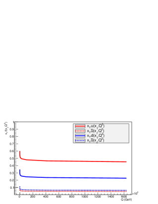
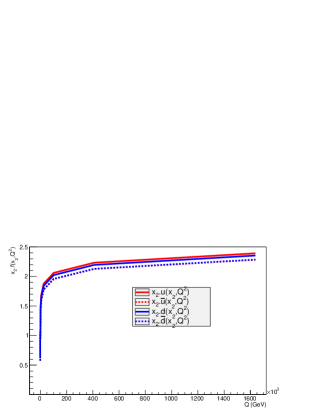
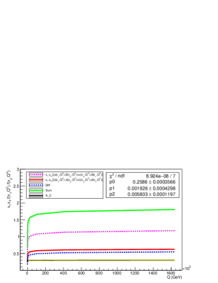
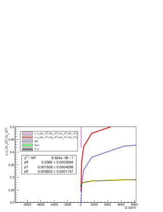
Figure 27: Evolutions of the quark PDFs (top), of the quark currents in the IS and of $A_{C}$ (bottom) calculated with QCDNUM using the MSTW2008nlo68cl parametrization.

A.2 Toy Models for the Main Properties of $A_{C}^{Fit}$

Hereafter, we make the hypothesis that quark currents and $A_{C}$ can be fitted by the different polynomials of functions of $Q$ evoked above. We want to figure out how the coefficients of such polynomials arrange so as to give the $A_{C}$ template curves presented in sub-section  2.1, i.e. monotonically increasing functions of $Q$ with a monotonically decreasing slope.

Again, let’s consider the simplest case where the first degree polynomials are sufficient. If we denote $x=Q$, and $f(x)$ the fit function, we can write the charged cross sections:

$$\begin{cases}\sigma^{+}(x)=P_{0}+P_{1}\cdot f(x)\\ \sigma^{-}(x)=M_{0}+M_{1}\cdot f(x)\\ \end{cases}$$ (60)

therefore

$$A_{C}(x)=\frac{(P_{0}-M_{0})+(P_{1}-M_{1})\cdot f(x)}{(P_{0}+M_{0})+(P_{1}+M_{1})\cdot f(x)}$$ (61)

Provided that $\lim\limits_{x\to+\infty}|f(x)|=+\infty$ (which holds for all the fit functions we considered), it appears that $A_{C}$ has an asymptote given by:

$$\lim\limits_{x\to+\infty}A_{C}(x)=\frac{(P_{1}-M_{1})}{(P_{1}+M_{1})}$$ (62)

The derivative of $A_{C}(x)$ can be expressed as:

$$\frac{dA_{C}(x)}{dx}=\frac{2\cdot(P_{1}M_{0}-P_{0}M_{1})\cdot f^{\prime}(x)}{[(P_{0}+M_{0})+(P_{1}+M_{1})\cdot f(x)]^{2}}$$ (63)

Hence the condition to get a monotonically increasing $A_{C}(x)$ writes:

$$\frac{dA_{C}(x)}{dx}\geq 0\Longleftrightarrow(P_{1}M_{0}-P_{0}M_{1})\cdot f^{\prime}(x)\geq 0$$ (64)

And finally, that fact that $A_{C}$ can be fitted with the same functional form as $\sigma^{+}(x)$ and $\sigma^{-}(x)$ relies on the (approximate) fullfilment of the following second degree functional equation:

$$(A_{1}M_{1})\cdot\left(f(x)\right)^{2}+(A_{0}M_{1}+A_{1}M_{0}-P_{1})\cdot f(x)+(A_{0}M_{0}-P_{0})=0$$ (65)

This equation has an analyitical solution if it’s determinant is positive or null:

$$\Delta=\sqrt{(A_{0}M_{1}+A_{1}M_{0}-P_{1})^{2}-4\cdot(A_{1}M_{1})\cdot(A_{0}M_{0}-P_{0})}\geq 0.$$

The fits of $\sigma^{+}(x)$, $\sigma^{-}(x)$ and $A_{C}$ with the 3 considered functional forms are performed and the corresponding values of the fit parameters are presented in table 58.

Fit Parameter	Polynomial	Polynomial	Laguerre
	of $Log(Q)$	of $Log\left(Log(Q)\right)$	Polynomials
$P_{0}$	$0.33\pm 0.03$	$0.01\pm 0.03$	$0.79\pm 0.08$
$P_{1}$	$0.064\pm 0.004$	$0.43\pm 0.02$	$(-2.9\pm 1.5)\times 10^{-7}$
$M_{0}$	$0.21\pm 0.02$	$0.04\pm 0.01$	$0.44\pm 0.04$
$M_{1}$	$0.032\pm 0.002$	$0.220\pm 0.006$	$(-1.4\pm 0.8)\times 10^{-7}$
$A_{0}$	$0.258\pm 0.002$	$0.242\pm 0.002$	$0.283\pm 0.004$
$A_{1}$	$0.0036\pm 0.0002$	$0.023\pm 0.001$	$(-1.6\pm 0.8)\times 10^{-8}$

Table 58: Values of the fits parameters.

A.2.1 Polynomials of $Log(x)$

In this case, our toy model writes:

$$A_{C}(x)=\frac{(P_{0}-M_{0})+(P_{1}-M_{1})\cdot Log(x)}{(P_{0}+M_{0})+(P_{1}+M_{1})\cdot Log(x)}$$ (66)

with

$$\frac{dA_{C}(x)}{dx}=\frac{2\cdot(P_{1}M_{0}-P_{0}M_{1})}{x\cdot[(P_{0}+M_{0})+(P_{1}+M_{1})\cdot Log(x)]^{2}}$$ (67)

and, since x > 0,

$$\frac{dA_{C}(x)}{dx}\geq 0\Longleftrightarrow(P_{1}M_{0}-P_{0}M_{1})\geq 0$$ (68)

Given the values of the fits parameters:

• the asymptoteic $A_{C}$ is $33.0\%$

• $P_{1}M_{0}-P_{0}M_{1}=2.51\times 10^{-3}\geq 0$

• $\Delta=3.12\times 10^{-3}\geq 0$

Therefore $A_{C}(x)$ can be fitted by a first order polynomial of $Log(x)$, it’s a monotonically increasing function, yet its has an asymptote.

A.2.2 Polynomials of $Log\left(Log(x)\right)$

In this case, our toy model writes:

$$A_{C}(x)=\frac{(P_{0}-M_{0})+(P_{1}-M_{1})\cdot Log\left(Log(x)\right)}{(P_{0}+M_{0})+(P_{1}+M_{1})\cdot Log\left(Log(x)\right)}$$ (69)

with

$$\frac{dA_{C}(x)}{dx}=\frac{2\cdot(P_{1}M_{0}-P_{0}M_{1})}{x\cdot Log(x)\cdot[(P_{0}+M_{0})+(P_{1}+M_{1})\cdot Log\left(Log(x)\right)]^{2}}$$ (70)

and, since x > 0 (in practice x > 10 GeV) and Log(x) > 0,

$$\frac{dA_{C}(x)}{dx}\geq 0\Longleftrightarrow(P_{1}M_{0}-P_{0}M_{1})\geq 0$$ (71)

Given the values of the fits parameters:

• the asymptotic $A_{C}$ is $32.6\%$

• $P_{1}M_{0}-P_{0}M_{1}=1.57\times 10^{-2}\geq 0$

• $\Delta=0.144\geq 0$

Therefore $A_{C}(x)$ can be fitted by a first order polynomial of $Log\left(Log(x)\right)$, it’s a monotonically increasing function, yet its has an asymptote.

A.2.3 Laguerre Polynomials $L_{n}(x)$

The toy model writes:

$$A_{C}(x)=\frac{(P_{0}-M_{0})+(P_{1}-M_{1})\cdot(1-x)}{(P_{0}+M_{0})+(P_{1}+M_{1})\cdot(1-x)}$$ (72)

with

$$\frac{dA_{C}(x)}{dx}=\frac{-2\cdot(P_{1}M_{0}-P_{0}M_{1})}{[(P_{0}+M_{0})+(P_{1}+M_{1})\cdot(1-x)]^{2}}$$ (73)

and,

$$\frac{dA_{C}(x)}{dx}\geq 0\Longleftrightarrow(P_{1}M_{0}-P_{0}M_{1})\leq 0$$ (74)

Given the values of the fits parameters:

• the asymptoteic $A_{C}$ is $34.2\%$

• $P_{1}M_{0}-P_{0}M_{1}=-1.46\times 10^{-3}\leq 0$

• $\Delta=6.3\times 10^{-14}\geq 0$

Therefore $A_{C}(x)$ can be fitted by a first order polynomial of $(1-x)$, it’s a monotonically increasing function, yet its has an asymptote.

We verified that for the case without longitudinal boost: $x_{1}=x_{2}=1.15\times 10^{-2}$, the conclusions listed above remain valid.

References

- (1) A. D. Martin, W. J. Stirling, R. S. Thorne and G. Watt, Eur. Phys. J. C 63 (2009) 189 [arXiv:0901.0002 [hep-ph]].
- (2) A. Cafarella, C. Coriano and M. Guzzi, Nucl. Phys. B 748 (2006) 253 [hep-ph/0512358].
- (3) G. Aad et al. [ATLAS Collaboration], Phys. Lett. B 701 (2011) 31 [arXiv:1103.2929 [hep-ex]].
- (4) S. Chatrchyan et al. [CMS Collaboration], Phys. Rev. Lett. 109 (2012) 111806 [arXiv:1206.2598 [hep-ex]].
- (5) S. Chatrchyan et al. [CMS Collaboration], arXiv:1312.6283 [hep-ex].
- (6) The LHCb Collaboration [LHCb Collaboration], “Updated measurements of and production at = 7 TeV with the LHCb experiment,” LHCb-CONF-2011-039.
- (7) [ATLAS Collaboration], ATLAS-CONF-2011-129.
- (8) L. Schoeffel, Nucl. Instrum. Meth. A 423 (1999) 439.
- (9) M. Botje, Comput. Phys. Commun. 182 (2011) 490 [arXiv:1005.1481 [hep-ph]].
- (10) A. Djouadi et al. [MSSM Working Group Collaboration], hep-ph/9901246.
-
(11)
S. Muanza, GDR SUSY Internal Note, May 2000. Unpublished.
http://susy.in2p3.fr/GDR-Notes/GDR_SUSY_PUBLIC/GDR-S-076.ps. - (12) G. P. Lepage, CLNS-80/447.
- (13) J. Alwall, P. Schuster and N. Toro, Phys. Rev. D 79 (2009) 075020 [arXiv:0810.3921 [hep-ph]].
- (14) B. Fuks, M. Klasen, D. R. Lamprea and M. Rothering, Eur. Phys. J. C 73 (2013) 2480 [arXiv:1304.0790 [hep-ph]].
- (15) C. Anastasiou, K. Melnikov and F. Petriello, “Fully differential Higgs boson production and the di-photon signal through next-to-next-to-leading order,” Nucl. Phys. B 724 (2005) 197 [arXiv:hep-ph/0501130].
- (16) S. Catani, L. Cieri, G. Ferrera, D. de Florian and M. Grazzini, “Vector boson production at hadron colliders: a fully exclusive QCD calculation at NNLO,” Phys. Rev. Lett. 103 (2009) 082001 [arXiv:0903.2120 [hep-ph]].
- (17) J. Pumplin, D. R. Stump, J. Huston, H. L. Lai, P. M. Nadolsky and W. K. Tung, JHEP 0207 (2002) 012 [hep-ph/0201195].
- (18) P. M. Nadolsky, H. L. Lai, Q. H. Cao, J. Huston, J. Pumplin, D. Stump, W. K. Tung and C.-P. Yuan, Phys. Rev. D 78 (2008) 013004 [arXiv:0802.0007 [hep-ph]].
- (19) A. Sherstnev and R. S. Thorne, Eur. Phys. J. C 55 (2008) 553 [arXiv:0711.2473 [hep-ph]].
- (20) A. D. Martin, R. G. Roberts, W. J. Stirling and R. S. Thorne, Phys. Lett. B 604 (2004) 61 [hep-ph/0410230].
- (21) T. Sjostrand, S. Mrenna and P. Z. Skands, “PYTHIA 6.4 Physics and Manual,” JHEP 0605 (2006) 026 [arXiv:hep-ph/0603175].
- (22) A.D. Martin, W.J. Stirling, R.S. Thorne, G. Watt, “Parton distributions for the LHC,” Eur. Phys. J. C63 (2009) 189-285.
- (23) J. M. Campbell, J. W. Huston and W. J. Stirling, “Hard Interactions of Quarks and Gluons: A Primer for LHC Physics,” Rept. Prog. Phys. 70 (2007) 89 [arXiv:hep-ph/0611148].
- (24) M. R. Whalley, D. Bourilkov and R. C. Group, hep-ph/0508110.
- (25) G. Miu and T. Sjostrand, Phys. Lett. B 449 (1999) 313 [arXiv:hep-ph/9812455].
- (26) C. Balazs, J. Huston and I. Puljak, Phys. Rev. D 63 (2001) 014021 [arXiv:hep-ph/0002032].
- (27) G. Aad et al. [ATLAS Collaboration], arXiv:1103.1816 [hep-ex].
- (28) K. Nakamura et al. [Particle Data Group], J. Phys. G 37 (2010) 075021.
- (29) S. Ovyn, X. Rouby and V. Lemaitre, arXiv:0903.2225 [hep-ph].
- (30) M. Dobbs, J. B. Hansen, Comput. Phys. Commun. 134 (2001) 41-46.
- (31) T. Schörner-Sadenius and S. Tapprogge, ATL-DAQ-2003-004.
- (32) M. Cacciari, G. P. Salam and G. Soyez, JHEP 0804 (2008) 063 [arXiv:0802.1189 [hep-ph]].
- (33) J. M. Campbell and R. K. Ellis, Phys. Rev. D 60 (1999) 113006 [arXiv:hep-ph/9905386].
- (34) J. M. Campbell and R. K. Ellis, Phys. Rev. D 62 (2000) 114012 [arXiv:hep-ph/0006304].
- (35) J. M. Campbell and R. K. Ellis, Phys. Rev. D 65 (2002) 113007 [arXiv:hep-ph/0202176].
- (36) W. Beenakker, M. Klasen, M. Kramer, T. Plehn, M. Spira and P. M. Zerwas, Phys. Rev. Lett. 83 (1999) 3780 [Erratum-ibid. 100 (2008) 029901] [arXiv:hep-ph/9906298].
- (37) W. Beenakker, M. Kramer, T. Plehn, M. Spira and P. M. Zerwas, Nucl. Phys. B 515 (1998) 3 [arXiv:hep-ph/9710451].
- (38) W. Beenakker, R. Hopker, M. Spira and P. M. Zerwas, Nucl. Phys. B 492 (1997) 51 [arXiv:hep-ph/9610490].
- (39) M. Spira, arXiv:hep-ph/0211145.
- (40) T. Plehn, Czech. J. Phys. 55 (2005) B213 [arXiv:hep-ph/0410063].
- (41) S. Gieseke et al., arXiv:1102.1672 [hep-ph].
- (42) http://cc.in2p3.fr/docenligne/13/en
- (43) J. Ohnemus, Phys. Rev. D 47, 940 (1993).
- (44) R. Hamberg, W. L. van Neerven and T. Matsuura, Nucl. Phys. B 359 (1991) 343 [Erratum-ibid. B 644 (2002) 403].
- (45) J. M. Campbell, R. Frederix, F. Maltoni and F. Tramontano, Phys. Rev. Lett. 102 (2009) 182003 [arXiv:0903.0005 [hep-ph]].
- (46) J. M. Campbell, R. K. Ellis and F. Tramontano, Phys. Rev. D 70 (2004) 094012 [arXiv:hep-ph/0408158].
- (47) R. Gavin, Y. Li, F. Petriello and S. Quackenbush, arXiv:1011.3540 [hep-ph].
- (48) S. Chatrchyan et al. [CMS Collaboration], JHEP 1110 (2011) 132 [arXiv:1107.4789 [hep-ex]].
-
(49)
Delphes ticket submitted and solved by S. Muanza,
https://cp3.irmp.ucl.ac.be/projects/delphes/ticket/44 -
(50)
M.L. Mangano,
http://mlm.web.cern.ch/mlm/talks/lund-alpgen.pdf - (51) M.L. Mangano, M. Moretti, F. Piccinini and M. Treccani, JHEP 0701 (2007) 013 [hep-ph/0611129].
- (52) K. Cranmer, Statistical Problems in Particle Physics, Astrophysics and CosmoLogy, Conf. Proc. (2006) 112
-
(53)
RooStats Tutorial, K. Cranmer (2009)
http://root.cern.ch/root/html/tutorials/roostats/rs_numbercountingutils.C.html. - (54) G. Aad et al. [ATLAS Collaboration], Eur. Phys. J. C 72 (2012) 2173 [arXiv:1208.1390 [hep-ex]].
- (55) G. Aad et al. [ATLAS Collaboration], ATLAS-CONF-2013-021.
- (56) G. Polesello and D. R. Tovey, JHEP 1003 (2010) 030 [arXiv:0910.0174 [hep-ph]].
- (57) D. R. Tovey, http://projects.hepforge.org/mctlib.
- (58) H. Baer, C. h. Chen, F. Paige and X. Tata, Phys. Rev. D 50 (1994) 4508 [hep-ph/9404212].
- (59) T. Aaltonen et al. [CDF Collaboration], Phys. Rev. D 83 (2011) 112003 [arXiv:1101.0034 [hep-ex]].
- (60) V. M. Abazov et al. [D0 Collaboration], Phys. Rev. D 84 (2011) 112005 [arXiv:1107.4995 [hep-ex]].
- (61) S. Knapen, Y. Zhao and M. J. Strassler, Phys. Rev. D 86 (2012) 014013 [arXiv:1111.5857 [hep-ph]].
- (62) S. Chatrchyan et al. [CMS Collaboration], Phys. Lett. B 717 (2012) 351 [arXiv:1206.3921 [hep-ex]].
- (63) N. Craig, C. Kilic and M. J. Strassler, Phys. Rev. D 84 (2011) 035012 [arXiv:1103.2127 [hep-ph]].
- (64) G. Aad et al. [ATLAS Collaboration], JHEP 1402 (2014) 107 [arXiv:1311.6724 [hep-ex]].
- (65) S. Chatrchyan et al. [CMS Collaboration], JHEP 1404 (2014) 191 [arXiv:1402.3803 [hep-ex]].
- (66) A. J. Barr, Phys. Lett. B 596 (2004) 205 [hep-ph/0405052].
- (67) J. M. Smillie and B. R. Webber, JHEP 0510 (2005) 069 [hep-ph/0507170].
- (68) T. Appelquist, H. C. Cheng and B. A. Dobrescu, Phys. Rev. D 64 (2001) 035002 [hep-ph/0012100].
- (69) S. Muanza [ATLAS Collaboration],
- (70) S. Muanza, In Turin 1996, Diquarks 3, 109-115
- (71) G. S. Muanza, PCCF-T-96-01.
- (72) H. Bachacou, I. Hinchliffe and F. E. Paige, Phys. Rev. D 62 (2000) 015009 doi:10.1103/PhysRevD.62.015009 [hep-ph/9907518].
- (73) G. Aad et al. [ATLAS Collaboration], Eur. Phys. J. C 74 (2014) 10, 3071 doi:10.1140/epjc/s10052-014-3071-4 [arXiv:1407.5063 [hep-ex]].
- (74) G. Aad et al. [ATLAS Collaboration], Eur. Phys. J. C 74 (2014) 11, 3130 doi:10.1140/epjc/s10052-014-3130-x [arXiv:1407.3935 [hep-ex]].
- (75) G. Aad et al. [ATLAS Collaboration], Eur. Phys. J. C 72 (2012) 2173 doi:10.1140/epjc/s10052-012-2173-0 [arXiv:1208.1390 [hep-ex]].
- (76) A. J. Barr and C. G. Lester, J. Phys. G 37 (2010) 123001 doi:10.1088/0954-3899/37/12/123001 [arXiv:1004.2732 [hep-ph]].
- (77) D. Curtin, Phys. Rev. D 85 (2012) 075004 doi:10.1103/PhysRevD.85.075004 [arXiv:1112.1095 [hep-ph]].
- (78) W. S. Cho, K. Choi, Y. G. Kim and C. B. Park, JHEP 0802 (2008) 035 doi:10.1088/1126-6708/2008/02/035 [arXiv:0711.4526 [hep-ph]].