Neural Network Regularization via Robust Weight Factorization

Abstract

Regularization is essential when training large neural networks. As deep neural networks can be mathematically interpreted as universal function approximators, they are effective at memorizing sampling noise in the training data. This results in poor generalization to unseen data. Therefore, it is no surprise that a new regularization technique, Dropout, was partially responsible for the now-ubiquitous winning entry to ImageNet 2012 by the University of Toronto. Currently, Dropout (and related methods such as DropConnect) are the most effective means of regularizing large neural networks. These amount to efficiently visiting a large number of related models at training time, while aggregating them to a single predictor at test time. The proposed FaMe model aims to apply a similar strategy, yet learns a factorization of each weight matrix such that the factors are robust to noise.

1 Introduction

Much of the recent surge in popularity in neural networks, especially in their application to classification of visual data, is due to advances in regularization. The winning entry in the 2012 ImageNet LSVRC-2012 challenge by Krizhevsky et al. (2012) used a deep convolutional neural network to surpass the competition by a margin of nearly 8% in top-5 test error rate. They partially attribute their performance to regularization technique called “Dropout” (Krizhevsky et al., 2012; Hinton et al., 2012; Srivastava et al., 2014). As large neural networks are extremely powerful, avoiding overfitting is crucial to increasing generalization performance. Dropout is an elegant and simple solution which is equivalent to training an exponential number of models. At test time, these models are ‘averaged’ into a single ‘mean’ predictor which generalizes better to unseen test data.

However, models with rectified linear activations (ReLU) are known to lead to sparse activations, with 50% percent of units with true zero activation (Glorot et al., 2011). Our experiments have shown that this number is as high as 75% when training with Dropout. Although sparse representations are desirable in general (Lee et al., 2008; Ranzato et al., 2007; 2008), they reduce the effective number and size of models that Dropout visits during training. In other words, the multiplicative noise applied by Dropout has no effect on the sparse activations. Ba et al. (2014) address this by adding an post-activation bias to the ReLU activation function, making explicit the distinction between sparse units and units masked by Dropout.

We propose a related regularization procedure which we call Factored Mean training (FaMe). From a high-level, FaMe is similar to Dropout. Both methods address the problem of overfitting by efficiently training an ensemble of models which are averaged together at test time. Where Dropout achieves this by randomly masking units, FaMe does so by learning a factorization of each weight matrix such that the factors are robust to noise. This leads to a more accurate model averaging procedure without sacrificing FaMe’s ability to make use of shared information between the models visited at training time.

2 Background

In this section, we briefly review traditional methods to improve generalization before discussing modern advances such as Dropout and Drop-connect. We also introduce the concept of gating: networks which achieve weight modulation via multiplicative interactions among variables.

2.1 Traditional approaches to improve generalization

Traditional approaches to improving generalization in neural networks can be seen as a means of limiting the capacity of the model. These include early stopping, weight decay ($L_{1}$ or $L_{2}$), weight constraints or the addition of noise to the during training. Where weight decay involves adding a proportional to the $L_{1}$ or $L_{2}$ norm of the weights to the objective, weight constraints limits the $L_{2}$ norm for the incoming weight vector of each unit (Hinton et al., 2012).

Addition of noise during training is also an effective regularizer (Bishop, 1995b; Vincent et al., 2008; Hinton & Van Camp, 1993). Adding small amounts of noise to the input vector has been shown to be equivalent to Tikhonov regularization (Bishop, 1995b). Denoising autoencoders (DAE) (Vincent et al., 2008) apply either additive or multiplicative (e.g. masking) noise to the input signal. The model then must learn to ‘denoise’ the input and reconstruct the uncorrupted input. The denoising criterion permits overcomplete models (i.e. models with more hidden units per layer than input units) to learn useful representations by way of predictive opposition between the reconstruction distribution and the regularizer (Vincent et al., 2010).

2.2 Dropout

Dropout (Hinton et al., 2012; Srivastava et al., 2014) was motivated by the idea that sexual reproduction increases the overall fitness of a species by preventing complex co-adaptations of genes. Likewise, Dropout aims to increase generalization performance by preventing complex co-adaptations of hidden units.

Formally, consider a feed forward neural network with $L$ hidden layers. Define $\mathbf{h}^{(l)}$ as the output vector from hidden layer $l$. The learning procedure learns a parameterized function $f(\mathbf{x})=\mathbf{y}$. Let $\mathbf{x}\in\mathbb{R}^{n^{x}}$ be the input vector, $\mathbf{h}^{(l)}\in\mathbb{R}^{n^{l}}$ be the hidden vector, and $\mathbf{y}\in\mathbb{R}^{n^{y}}$ the output vector where $n^{x},n^{l},n^{y}$ are the number of input, hidden (for layer $l$) and output dimensions. By convention, we define $\mathbf{h}^{(0)}=\mathbf{x}$ and $\mathbf{h}^{(L+1)}=\mathbf{y}$. Next, define $\mathbf{W}^{(l)}\in\mathbb{R}^{n^{l}\times n^{l-1}}$ as the weights and $\mathbf{b}^{(l)}\in\mathbb{R}^{n^{l}}$ as the hidden biases for layer $l$. The hidden unit and output activations can be written as

$$\mathbf{h}^{(l)}=\sigma^{(l)}\left(\mathbf{W}^{(l)}\mathbf{h}^{(l-1)}+\mathbf{b}^{(l)}\right)$$ (1)

$$f(\mathbf{x})=\mathbf{y}=\sigma^{(y)}\left(\mathbf{W}^{(L+1)}\mathbf{h}^{(L)}+\mathbf{b}^{(L+1)}\right)$$ (2)

where $\sigma^{(l)},\sigma^{(y)}$ are the hidden and output activation functions. The weight matrices and bias vectors are randomly initialized and learned via optimization of a cost function, typically via gradient descent.

Under Dropout, multiplicative noise is applied to the hidden activations during training for each presentation of an input. This is accomplished by stochastically dropping (or masking) individual hidden units in each layer (Srivastava et al., 2014). Formally, define $\mathbf{r}^{(l)}\in\mathbb{R}^{n^{l}}$ such that $r^{(l)}_{i}\sim\text{Bernoulli}(p)$, i.e. $\mathbf{r}^{(l)}$ is a vector of independent Bernoulli variables where each has probability $p$ of being 1 (Srivastava et al., 2014). During training, Equation 1 becomes

$$\hat{\mathbf{h}}^{(l)}=\sigma^{(l)}\left(\mathbf{W}^{(l)}\left(\mathbf{h}^{(l-1)}\circ\mathbf{r}^{(l-1)}\right)+\mathbf{b}^{(l)}\right)$$ (3)

where $\circ$ denotes the elementwise product. No masking is performed at test time. In order to compensate for the lack of masking, the weights are scaled by $p$ once training is complete (Srivastava et al., 2014). Recent results have shown that using Gaussian noise with $\mu=1$ (as opposed to Bernoulli) leads to improved test performance (Srivastava et al., 2014). At test time each $r_{i}=\mu=1$ and, as such, the weights of the testing model do not require scaling.

The Bernoulli Dropout procedure can be interpreted as a means of training a different sub-network for each training example, where each sub-network contains a subset of the connections in the model. There is an exponential number of such networks, and many may not be visited during training. However, the extensive amount of weight sharing between these networks allows them to make useful predictions regardless of the fact that they may have not been trained explicitly (Hinton et al., 2012). Under this interpretation, the test procedure can be seen as an approximation of the geometric average of all the sub-networks (Srivastava et al., 2014).

Dropout has inspired a variety of both theoretical and experimental research. Subsequent theoretical work has found that training with Dropout is equivalent to an adaptive version of $L_{2}$ weight decay (Wager et al., 2013). Where the traditional $L_{2}$ penalty is spherical in weight space, Dropout is akin to an axis aligned scaling of the $L_{2}$ penalty such that it takes the curvature of the likelihood function into account (Wager et al., 2013). An extension of Dropout, DropConnect, applies the mask not to the hidden units but to the connections between units and was found to outperform Dropout on certain image recognition tasks (Wan et al., 2013). Maxout networks (Goodfellow et al., 2013) are an attempt to design a new type of activation function which exploits the benefits of the Dropout training procedure.

2.3 Gated Models

Where classical neural networks contain only first order interactions among input variables and hidden variables, gated models permit a tri-partite graph that connects hidden variables to pairs of input variables. The messages sent in such networks involve multiplicative interactions among variables and permit the learning of structure in the relationship between inputs rather than the structure of inputs themselves (Memisevic & Hinton, 2007; Taylor & Hinton, 2009; Memisevic, 2013). Recent applications of such models include modeling transformations between images (Memisevic, 2013), 3D depth (Konda & Memisevic, 2013), and time-series data (Michalski et al., 2014).

The objective of a typical first order neural network is to learn a mapping function between an input $\mathbf{x}$ and an output $\mathbf{y}$. In other words, training involves updating the model weights such that the model learns the function $f(\mathbf{x})=\mathbf{y}$. Instead of learning a mapping between a single input and output vector, gated models are conditional on a second input $\mathbf{z}$ such that the learned function is $f(\mathbf{x}|\mathbf{z})=\mathbf{y}$. We refer to $\mathbf{z}$ as the “context”. Instead of a fixed weight matrix as in classical neural networks, the weights in a gated model can be interpreted as being a function of the context $\mathbf{z}$ (Memisevic, 2013).

Formally, the hidden activation in a single layered factored gated model with input vectors $\mathbf{x}\in\mathbb{R}^{n^{x}}$, context $\mathbf{z}\in\mathbb{R}^{n^{z}}$ and factor size $n^{f}$

$$\mathbf{h}=f(\mathbf{x}|\mathbf{z})=\sigma^{(h)}\left(\mathbf{W}^{T}\left(\mathbf{U}\mathbf{x}\circ\mathbf{V}\mathbf{z}\right)+\mathbf{b}^{(h)}\right)$$ (4)

where $\mathbf{U}\in\mathbb{R}^{n^{f}\times n^{x}}$, $\mathbf{V}\in\mathbb{R}^{n^{f}\times n^{z}}$, $\mathbf{W}\in\mathbb{R}^{n^{f}\times n^{h}}$ are learned weight matrices, $\mathbf{b}^{(h)}\in\mathbb{R}^{n^{h}}$ are the hidden biases, $\circ$ denotes an elementwise product, and $\sigma^{(h)}$ is the hidden activation function (typically of the sigmoidal family or piecewise linear).

Note that in the special case where $\mathbf{z}$ is constant, Equation 4 becomes

$$\mathbf{h}=\hat{f}(\mathbf{x})=\sigma^{(h)}\left(\hat{\mathbf{W}}\mathbf{x}+\mathbf{b}^{(h)}\right)$$ (5)

where $\hat{\mathbf{W}}=\left(\mathbf{W}\circ\left(\left(\mathbf{V}\mathbf{z}\right)\otimes\mathbf{e}\right)\right)\mathbf{U}$, such that $\mathbf{e}$ is a $n^{h}$ dimensional vector of ones and $\otimes$ is the Kronecker product. Thus, with constant $\mathbf{z}$ the gated model is equivalent to a feed forward model.

3 FaMe Training

The proposed Factored Mean training procedure (FaMe) aims to make use of the weight modulation property of gated networks as a means of regularization. The FaMe architecture, like a neural network trained with Dropout, aims to learn a mapping $f(\mathbf{x})=\mathbf{y}$ between input $\mathbf{x}$ and output vector $\mathbf{y}$ (e.g. for classification). Where Dropout applies multiplicative noise to the hidden activations during training, under FaMe training each weight matrix is decomposed into two matrices (or “factor loadings”) and the multiplicative noise is applied directly after the input vector is projected onto the first of these matrices.

Formally, given a feed forward neural network with $L$ layers as described in section 2.2, instead of a single weight matrix $\mathbf{W}^{(l)}$ for layer $l$ we define matrices $\mathbf{U}^{(l)}\in\mathbb{R}^{f^{l}\times n^{(l-1)}}$, $\mathbf{V}^{(l)}\in\mathbb{R}^{n^{l}\times f^{l}}$ where $f^{l}$ is a free parameter. Thus, the hidden activation becomes

$$\mathbf{h}^{(l)}=\sigma^{(l)}\left(\mathbf{V}^{(l)}\left(\mathbf{U}^{(l)}\mathbf{h}^{(l-1)}\circ\mathbf{r}^{(l)}\right)+\mathbf{b}^{(l)}\right)$$ (6)

where $\mathbf{r}^{(l)}\in\mathbb{R}^{f^{l}}$. During training, each $r_{i}^{(l)}$ is an independent sample from a fixed probability distribution (i.e. Bernoulli, Gaussian). See Figure 1 for a comparison of the FaMe architecture and a classical feed forward model.

Note the similarity between Equation 6 and the gated model Equation 4. Instead of the model weights being a function of a secondary input vector $\mathbf{z}$, the FaMe training procedure modulates the weights via a random vector $\mathbf{r}^{(l)}$. Like Dropout, the FaMe model can be viewed as training a unique model for each training example and epoch. In other words, the FaMe model represents a manifold of models where the settings of $(\mathbf{r}^{(1)},\mathbf{r}^{(2)},\ldots\mathbf{r}^{(L+1)})$ can be thought of as the coordinates of a given model on that manifold.

Where Dropout computes an average mean network by scaling the weights by $p$, at test time we can calculate the mean network learned by FaMe training by setting each $r^{(l)}_{i}$ to the expectation of its sampling distribution. This is similar to Equation 5 when we fix secondary input in the gated model. However, if we define $r_{i}^{(l)}\sim N(1,1)$ (or any other distribution with mean 1), then our hidden activations in our mean network at test time can be simplified to

$$\mathbf{h}^{(l)}=\sigma^{(l)}\left(\mathbf{W}^{(l)}\mathbf{h}^{(l-1)}+\mathbf{b}^{(l)}\right)\\$$ (7)

where $\mathbf{W}^{(l)}=\mathbf{V}^{(l)}\mathbf{U}^{(l)}$ (so, $\mathbf{W}^{(l)}\in\mathbb{R}^{n^{l}\times n^{(l-1)}}$). This is equivalent to Equation 1 of a classical feed forward network. In effect, the FaMe training procedure learns a decomposition of the weight matrix $\mathbf{W}^{(l)}$ such that it is robust to noise. Notice that in the process of learning a decomposition of $\mathbf{W}^{(l)}$, the rank of $\mathbf{W}^{(l)}$ can be bounded via the choice of $f^{l}$. In order to not restrict the rank of $\mathbf{W}^{(l)}$ and not introduce any unnecessary parameters, we can set $f^{l}=\min(n^{l},n^{(l-1)})$.

The parameters in the FaMe model can be learned using the same gradient-based optimization methods as a classical neural network.

3.1 FaMe Convolution layers

A similar technique can be applied to convolution layers, where a single convolution step can be decomposed into two linear convolution operations. Under FaMe training, multiplicative noise can be applied after the first convolution. This is similar to the Network in Network (NIN) model (Lin et al., 2014). Where each filter in NIN can be seen as a small non-linear MLP, in a FaMe convolution layer the filters are two layer linear networks with multiplicative noise added after the first layer.

Figure 1: Comparison of a classical feed forward neural network and FaMe. The figure on the right depicts the connectivity between hidden layers in a typical feed forward neural network. On the left is the connectivity between hidden layers in a FaMe model where $\mathbf{f}^{(l)}=\mathbf{U}^{(l)}\mathbf{h}^{(l-1)}$ and $\mathbf{r}^{(l)}$ is a vector in independent samples from some noise distribution. Biases are omitted for clarity.

4 Experiments

The effectiveness of the FaMe training procedure for image classification was evaluated on the MNIST (LeCun & Cortes, 1998) and CIFAR datasets (Krizhevsky & Hinton, 2009).

4.1 MNIST

The MNIST dataset consists of 60,000 training and 10,000 test examples, each of which is a 28 $\times$28 greyscale image of a handwritten digit. The training set was further randomly partitioned into a 50,000 image training set and a 10,000 image validation set.

Experiments were implemented in Python using the Theano library (Bastien et al., 2012; Bergstra et al., 2010). The model hyper-parameters were chosen based on performance on the validation set. During training, multiplicative Gaussian noise was a applied to both the input ($\sim\mathcal{N}(1,0.5)$) and linear factor layers ($\sim\mathcal{N}(1,1)$). Incoming weight vectors for each unit were constrained to a maximum $L_{2}$ norm of 2.0. Training was performed using mini-batch gradient descent on cross-entropy loss with a batch size of 250. Learning rates were annealed by a factor of 0.995 for each epoch. Nesterov accelerated gradient (Sutskever et al., 2013) was used for optimization, with initial value of 0.5 and increasing linearly for a set number of epochs. The final momentum value along with the number of epochs until reaching the final momentum value were chosen based on validation performance.

Training was performed for 500,000 weight updates (i.e. minibatches). The hyper-parameters which resulted in the lowest validation error were then used to train the final model on all 60,000 training examples. Again the test model was trained for a total of 500,000 weight updates.

Results on MNIST data are summarized in Table 1. Using the best settings of the hyper-parameters found during validation, the test model was trained from 10 random initializations and the average error of the ten models is reported. FaMe training outperforms Dropout (Srivastava et al., 2014) and Maxout (Goodfellow et al., 2013), achieving a best test error of $0.91\%(\pm 0.02)$. We found that restricting the rank of $W$ was beneficial with larger hidden layer sizes, where the two layer model restricted the size of the linear factor layer to 440. Additionally, training a model with fewer parameters achieves similar results. If we consider the size of the test model (after the $U$ and $V$ linear projections have been collapsed to as single weight matrix $W$) a FaMe model with 3 hidden layers with 512 units per layer has $\sim$93K effective parameters. The maxout model has $\sim$2.3 million free parameters and Gaussian Dropout has $\sim$1.9 million parameters.

Method	Unit Type	Architecture	Test Error %
Bernoulli Dropout NN + weight constraints	ReLU	2 layers, 8192 units	0.95
(Srivistava et al., 2014)
Bernoulli Dropout NN + weight constraints	Maxout	2 layers, (5x240) units	0.94
(Goodfellow et al., 2013)
Gaussian Dropout NN + weight constraints	ReLU	2 layers, 1024 units	0.95 +/- 0.05
(Srivistava et al., 2014)
Gaussian FaMe NN + weight constraints	ReLU	2 layers, 1024 units	0.91 +/- 0.02
Gaussian FaMe NN + weight constraints	ReLU	3 layers, 512 units	0.92 +/- 0.04

Table 1: Result of MNIST classification task. FaMe training outperforms dropout, even when training models with far fewer parameters.

4.2 CIFAR

The CIFAR datasets (Krizhevsky & Hinton, 2009) contain 60,000 $32\times 32$ color images, 50,000 of which are training examples with the remaining 10,000 used for testing. The CIFAR-10 dataset contains images from 10 classes where the CIFAR-100 contains 100 classes. Hyper-parameter selection followed a similar procedure to that used above for MNIST classification, further partitioning the training set into 40,000 training and 10,000 validation images. Our CIFAR models consist of three convolutional FaMe layers followed by two fully connected FaMe layers. The results are summarized in Table 2. For image preprocessing, we follow the same procedure as Srivastava et al. (2014) and Goodfellow et al. (2013). Global contrast normalization over each color channel is followed by ZCA whitening.

Although FaMe fails to outperform Dropout or Maxout, it is competitive with other recent results on CIFAR-10 and CIFAR-100. The discrete subset of parameters we considered for hyper-parameter cross-validation was substantially smaller than those considered for the MNIST task. We expect that with more time to optimize the parameters, potentially using tools such as Bayesian hyper-parameter optimization (Snoek et al., 2012), performance will improve.

Method	CIFAR-10 Error %	CIFAR-100 Error %
Conv Net + Spearmint (Snoek et al., 2012)	14.98	-
Conv Net + Dropout (fully connected) (Srivastava et al., 2014)	14.32	41.26
Conv Net + Dropout (all layers) (Srivastava et al., 2014)	12.61	37.20
Conv Net + Maxout (Goodfellow et al., 2013)	11.68	38.57
Conv Net + FaMe	12.85	39.79

Table 2: Comparison of FaMe training with other models on the CIFAR-10 dataset

5 Comparison with Dropout training

We conducted a separate set of experiments on MNIST to further probe the learning dynamics of FaMe vs. Dropout. All experiments described in this section were performed using a model with two non-linear (ReLU) hidden layers and multiplicative Gaussian noise from $\mathcal{N}(1,0.5)$ on the input and $\mathcal{N}(1,1)$ on the hiddens or factors. For both FaMe and Dropout training, hyper-parameters were chosen based on validation set performance.

5.1 Avoiding Overfitting

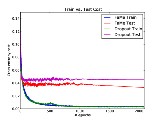
Figure 2: Training cost vs. test cost as training progresses on an example training run for both FaMe and Dropout. Notice that with FaMe training, the test cost continues to decrease for the entire duration of training.

Similar to Dropout training (Srivastava et al., 2014), FaMe training prevents overfitting and, as such, does not require early stopping. As seen in Figure 2 the test cost continues to decrease for the entirety of training. Dropout is also successful at avoiding overfitting, i.e. the test cost does not increase with continued training. However, the test cost plateaus earlier than with FaMe training.

5.2 Mean testing procedure

A full mathematical analysis of the mean test procedure given in Equation 7 is difficult due to the non-linearity of the hidden units. As such, we experimentally verify that the testing procedure is indeed approximating a geometric mean of predictions of the noisy subnetworks visited during training. Using the test data as input, we generate samples output from these noisy networks. The mean prediction can be calculated by first computing the geometric mean of the sample outputs and comparing to the output given by our deterministic testing procedure.

Figure 3 demonstrates that the FaMe testing procedure gives an accurate estimate of the true geometric mean of all subnetworks. By comparison, even though the Dropout test procedure outperforms the estimated geometric mean of the subnetworks, it does not provide a good estimate of the true mean network.

Note that both the FaMe and Dropout models contained two non-linear (ReLU) hidden layers and were trained with multiplicative Gaussian noise. Interestingly, the arithmetic mean prediction of the FaMe subnetworks appears to slightly outperform geometric mean prediction which may warrant further investigation.

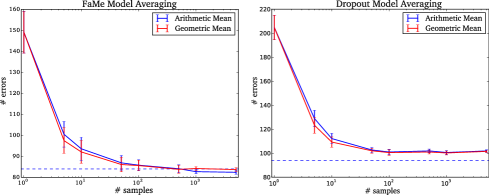
Figure 3: Comparison of the FaMe and Dropout test procedure to the true arithmetic and geometric means as estimated via sampling outputs of random subnetworks. With FaMe training (left), the prediction of the testing procedure (dashed blue line) does in fact give a good estimate of the true geometric mean prediction.

5.3 Adaptive $L_{2}$ weight decay

Wager et al. (2013) have shown Dropout to be equivalent to adaptive $L_{2}$ weight decay. To examine the link between weight decay and both FaMe and Dropout training, we monitor the $L_{2}$ norms of the weight matrices of under both training regimes. Figure 4 depicts the evolution of the $L_{2}$ norm of each $W$ weight matrix during training, relative to $L_{2}$ norm of its initial value (i.e. before training). Note that under FaMe trianing, we plot the $L_{2}$ norm of the implied weight matrix $W=VU$, where $V$ and $U$ are the factored weights that are actually learned by the model. Although no explicit $L_{2}$ penalty was used, both FaMe and Dropout training seem to impose an implicit penalty on the $L_{2}$ norm of the weight matrices. However, the effect is more pronounced under FaMe training.

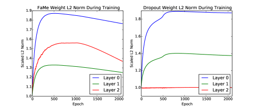
Figure 4: $L_{2}$ Norm of weight matrices during training. For visualization the $L_{2}$ norms are scaled by their value at initialization. Both training procedures exhibit behavior similar to $L_{2}$ weight decay, but the result is more pronounced in the case of FaMe training.

6 Conclusion

Regularization is essential when training large neural networks. Their power as universal function approximators allows them to memorize sampling noise in the training data, leading to poor generalization to unseen data. Traditional forms of generalization are means of limiting the model’s capacity. These include early stopping, weight decay, weight constraints, and addition of noise. Currently, Dropout (and related methods such as DropConnect) are the most effective means of regularizing large neural networks. These amount to efficiently visiting a large number of related models at training time, while aggregating them to a single mean model at test time. The proposed FaMe model aims to apply this same reasoning, but can be interpreted as a special form of weight-modulating, gated architecture.

Like Dropout, FaMe visits a family of models during training while allowing an efficient testing procedure for making predictions. Models trained with FaMe outperform Dropout training, even when such models have an order of magnitude fewer effective parameters. Additionally, restricting the rank of the factor loadings can be used as a means of controlling the number of free parameters. This is supported by recent work has looked closely at the significant redundancy in the parameterization of deep learning architectures, and proposed low-rank weight matrices as a way to massively reduce parameters while preserving predictive accuracy (Denil et al., 2013).

References

- Ba et al. (2014) Ba, Jimmy, Xiong, Hui Yuan, and Frey, Brendan. Making dropout invariant to transformations of activation functions and inputs. In NIPS 2014 Workshop on Deep Learning, 2014.
- Bastien et al. (2012) Bastien, Frédéric, Lamblin, Pascal, Pascanu, Razvan, Bergstra, James, Goodfellow, Ian J., Bergeron, Arnaud, Bouchard, Nicolas, and Bengio, Yoshua. Theano: new features and speed improvements. Deep Learning and Unsupervised Feature Learning NIPS 2012 Workshop, 2012.
- Bergstra et al. (2010) Bergstra, James, Breuleux, Olivier, Bastien, Frédéric, Lamblin, Pascal, Pascanu, Razvan, Desjardins, Guillaume, Turian, Joseph, Warde-Farley, David, and Bengio, Yoshua. Theano: a CPU and GPU math expression compiler. In SciPy, June 2010. Oral Presentation.
- Bishop (1995a) Bishop, Christopher M. Pattern recognition and machine learning, volume 1. Clarendon Press, Oxford, 1995a.
- Bishop (1995b) Bishop, Christopher M. Training with noise is equivalent to tikhonov regularization. Neural computation, 7(1):108–116, 1995b.
- Denil et al. (2013) Denil, Misha, Shakibi, Babak, Dinh, Laurent, de Freitas, Nando, et al. Predicting parameters in deep learning. In NIPS, 2013.
- Geman et al. (1992) Geman, Stuart, Bienenstock, Elie, and Doursat, René. Neural networks and the bias/variance dilemma. Neural computation, 4(1):1–58, 1992.
- Glorot et al. (2011) Glorot, Xavier, Bordes, Antoine, and Bengio, Yoshua. Deep sparse rectifier networks. In Proceedings of the 14th International Conference on Artificial Intelligence and Statistics. JMLR W&CP Volume, volume 15, pp. 315–323, 2011.
- Goodfellow et al. (2013) Goodfellow, Ian J, Warde-Farley, David, Mirza, Mehdi, Courville, Aaron, and Bengio, Yoshua. Maxout networks. arXiv preprint arXiv:1302.4389, 2013.
- Hinton (1987) Hinton, Geoffrey E. Learning translation invariant recognition in a massively parallel networks. In PARLE Parallel Architectures and Languages Europe, pp. 1–13. Springer, 1987.
- Hinton & Van Camp (1993) Hinton, Geoffrey E and Van Camp, Drew. Keeping the neural networks simple by minimizing the description length of the weights. In Proceedings of the sixth annual conference on Computational learning theory, pp. 5–13. ACM, 1993.
- Hinton et al. (2012) Hinton, Geoffrey E, Srivastava, Nitish, Krizhevsky, Alex, Sutskever, Ilya, and Salakhutdinov, Ruslan R. Improving neural networks by preventing co-adaptation of feature detectors. arXiv preprint arXiv:1207.0580, 2012.
- Hornik et al. (1989) Hornik, Kurt, Stinchcombe, Maxwell, and White, Halbert. Multilayer feedforward networks are universal approximators. Neural networks, 2(5):359–366, 1989.
- Konda & Memisevic (2013) Konda, Kishore and Memisevic, Roland. Learning to combine depth and motion. arXiv preprint arXiv:1312.3429, 2013.
- Krizhevsky & Hinton (2009) Krizhevsky, Alex and Hinton, Geoffrey. Learning multiple layers of features from tiny images. Computer Science Department, University of Toronto, Tech. Rep, 2009.
- Krizhevsky et al. (2012) Krizhevsky, Alex, Sutskever, Ilya, and Hinton, Geoffrey E. Imagenet classification with deep convolutional neural networks. In NIPS, 2012.
- LeCun & Cortes (1998) LeCun, Yann and Cortes, Corinna. The mnist database of handwritten digits, 1998.
- Lee et al. (2008) Lee, Honglak, Ekanadham, Chaitanya, and Ng, Andrew Y. Sparse deep belief net model for visual area v2. In NIPS, 2008.
- Lin et al. (2014) Lin, Min, Chen, Qiang, and Yan, Shuicheng. Network in network. In ICLR, 2014.
- Memisevic (2013) Memisevic, Roland. Learning to relate images. Pattern Analysis and Machine Intelligence, IEEE Transactions on, 35(8):1829–1846, 2013. ISSN 0162-8828. doi: 10.1109/TPAMI.2013.53.
- Memisevic & Hinton (2007) Memisevic, Roland and Hinton, Geoffrey. Unsupervised learning of image transformations. In CVPR, 2007.
- Michalski et al. (2014) Michalski, Vincent, Memisevic, Roland, and Konda, Kishore. Modeling sequential data using higher-order relational features and predictive training. arXiv preprint arXiv:1402.2333, 2014.
- Ranzato et al. (2007) Ranzato, Marc’Aurelio, Poultney, Christopher, Chopra, Sumit, and Cun, Yann L. Efficient learning of sparse representations with an energy-based model. In NIPS. 2007.
- Ranzato et al. (2008) Ranzato, Marc’Aurelio, lan Boureau, Y, and Cun, Yann L. Sparse feature learning for deep belief networks. In NIPS. 2008.
- Snoek et al. (2012) Snoek, Jasper, Larochelle, Hugo, and Adams, Ryan P. Practical bayesian optimization of machine learning algorithms. In Advances in Neural Information Processing Systems, pp. 2951–2959, 2012.
- Srivastava et al. (2014) Srivastava, Nitish, Hinton, Geoffrey, Krizhevsky, Alex, Sutskever, Ilya, and Salakhutdinov, Ruslan. Dropout: A simple way to prevent neural networks from overfitting. The Journal of Machine Learning Research, 15(1):1929–1958, 2014.
- Sutskever et al. (2013) Sutskever, Ilya, Martens, James, Dahl, George, and Hinton, Geoffrey. On the importance of initialization and momentum in deep learning. In ICML, 2013.
- Taylor & Hinton (2009) Taylor, Graham W and Hinton, Geoffrey E. Factored conditional restricted boltzmann machines for modeling motion style. In ICML, 2009.
- Tibshirani (1996) Tibshirani, Robert. Regression shrinkage and selection via the lasso. Journal of the Royal Statistical Society. Series B (Methodological), pp. 267–288, 1996.
- Vincent et al. (2008) Vincent, Pascal, Larochelle, Hugo, Bengio, Yoshua, and Manzagol, Pierre-Antoine. Extracting and composing robust features with denoising autoencoders. In ICML, 2008.
- Vincent et al. (2010) Vincent, Pascal, Larochelle, Hugo, Lajoie, Isabelle, Bengio, Yoshua, and Manzagol, Pierre-Antoine. Stacked denoising autoencoders: Learning useful representations in a deep network with a local denoising criterion. The Journal of Machine Learning Research, 9999:3371–3408, 2010.
- Wager et al. (2013) Wager, Stefan, Wang, Sida, and Liang, Percy. Dropout training as adaptive regularization. In NIPS, 2013.
- Wan et al. (2013) Wan, Li, Zeiler, Matthew, Zhang, Sixin, Cun, Yann L., and Fergus, Rob. Regularization of neural networks using dropconnect. In ICML, 2013.