Theory of temporal fluctuations in isolated quantum systems

Abstract

When an isolated quantum system is driven out of equilibrium, expectation values of general observables start oscillating in time. This article reviews the general theory of such temporal fluctuations. We first survey some results on the strength of such temporal fluctuations. For example temporal fluctuations are exponentially small in the system’s volume for generic systems whereas they fall-off algebraically in integrable systems. We then concentrate on the the so-called quench scenario where the system is driven out-of-equilibrium under the application of a sudden perturbation. For sufficiently small perturbations, temporal fluctuations of physical observables can be characterized in full generality and can be used as an effective tool to probe quantum criticality of the underlying model. In the off-critical region the distribution becomes Gaussian. Close to criticality the distribution becomes a universal function uniquely characterized by a single critical exponent, that we compute explicitly. This contrasts standard equilibrium quantum fluctuations for which the critical distribution depends on a numerable set of critical coefficients and is known only for limited examples. The possibility of using temporal fluctuations to determine pseudo-critical boundaries in optical lattice experiments is further reviewed.

1 Introduction

In the last few years we have witnessed a strong revival of interest in foundational issues of quantum statistical mechanics [1, 2, 3, 4, 5, 6, 7, 8, 9]. The central questions of this field go back to the time of Boltzmann: how do closed quantum systems out-of-equilibrium eventually equilibrate? Under which circumstances can we justify the amazing effectiveness of statistical ensembles in predicting the equilibrium properties of macroscopic observables in physical systems? Whereas understanding of thermal equilibrium is possible in the framework of quantum statistical mechanics we still do not know how thermal equilibrium is reached following the microscopic dynamical laws. What are the time-scales associated to thermalization, and what are the conditions leading to it? To date, even such simple questions lack a precise answer. Thanks to current advances in experimental techniques, isolated quantum systems are now routinely observed and the emergence of equilibrium can be experimentally put to test (see e.g. [10, 11, 12]). Motivated by such experiments there has been a tremendous effort in understanding how thermal equilibrium is reached. However, despite the sheer amount of results which have accumulated, the precise conditions which lead to thermalization remain to a large extent, unknown.

Understanding how thermalization is achieved amounts to understand two conceptually separate physical processes. On the one hand an “equilibrium” state emerges out of the dynamical evolution. This equilibration process is potentially much more general than thermalization itself. On the other hand one asks how and why this equilibrium state has the familiar thermal form expected from statistical mechanics, i.e. is a microcanonical, Gibbs, or grandcanonical thermal state depending on the appropriate ensemble. Indeed a great effort has been put in understanding the latter question. One of the central mechanisms that have been proposed is the so called Eigenstate Thermalization Hypothesis [13, 14, 15, 6] (see also [16] and the recent [17] for a comprehensive review). In this article however, we will concentrate on the equilibration process alone and will not be concerned if equilibration is of thermal type.

The first question we address is then, in which sense an equilibrium state can emerge out of a unitary dynamics? As it will be discussed in Sec. 2, equilibration in finite systems (or more generally in systems with discrete spectrum) must be formulated in a probabilistic fashion. In an out-of-equilibrium system, the expectation value of a quantum observable $A$, becomes a time-dependent quantity $\mathsf{A}(t):=\langle A(t)\rangle$ oscillating around an average value. In the spirit of the ergodic theory, one must introduce a large observation time window $[0,T]$. The time-fluctuations of $\langle A(t)\rangle$ are conveniently characterized by a temporal probability distribution function $P_{A}(a)$ where the full time statistics of $\langle A(t)\rangle$ is encoded. $P_{A}(a)da$ is the probability that $\langle A(t)\rangle\in[a,a+da]$ for $t$ in the observation window. Denoting with $\overline{f}=T^{-1}\int_{0}^{T}f(t)dt$ the time average operation, the equality $\overline{\mathsf{A}}:=\overline{\langle A(t)\rangle}=\mathrm{tr}(A\overline{\rho})$ shows that $\overline{\rho}$ plays the role of equilibrium state. Observables expectation values, $\mathsf{A}(t)$, oscillate around their averages $\overline{\mathsf{A}}$ with certain fluctuations encoded in the distributions $P_{A}(a)$. We can say that equilibration is reached if such fluctuations are small in some sense. In essence, equilibration in closed, finite, quantum systems, corresponds to concentration results (i.e the "peakedness") of these probability distributions $P_{A}(a)$. The purpose of these article is to illustrate that a wealth of physical information can be revealed from the study of the full time statistics. In well defined scenarios, the analysis of the full time statistics allows one to spot the precise location of the underlying quantum critical points [18, 19], or the integrable-non-integrable transition[20]. In general, the full temporal statistics of a given observable is an experimentally accessible quantity that encodes the physical data in a convenient way. In the sequel we will use natural units throughout in which $\hbar=k_{B}=1$.

2 Equilibration in closed quantum systems

Let us now lay down the setup of the problem in a general and formal way. The closed-system dynamics is described by the time-evolution operator $U(t)=e^{-itH}$. Let also $H=\sum_{n}E_{n}\Pi_{n}$ be the spectral resolution of the system Hamiltonian ($\Pi_{n}$’s spectral projections). Closed quantum systems evolve unitarily and therefore cannot converge in a strong sense to an equilibrium state starting out from a generic pure state. Indeed, call $\overline{\rho}$ the equilibrium state. $\overline{\rho}$ must be a fixed point of the dynamics, i.e. $U(t)\overline{\rho}U(t)^{\dagger}=\overline{\rho}$. But then, calling $\rho(t)=U(t)\rho_{0}U(t)^{\dagger}$, one has $\left\|\rho(t)-\overline{\rho}\right\|=\left\|\rho(t)-U(t)\overline{\rho}U(t)^{\dagger}\right\|=\left\|\rho_{0}-\overline{\rho}\right\|=\mathrm{const}.$ In words, the distance between the state at at time $t$ and the equilibrium state is constant. Despite of this fact, for sufficiently large system sizes one may observe temporal typicality. Namely, for the overwhelming majority of the time instants, the statistics of observables are practically indistinguishable from an effective equilibrium state. In this sense, equilibration in isolated quantum systems emerges in a probabilistic fashion.

One may then wonder whether a weaker form of convergence can be achieved for $t\to\infty$. Let us therefore consider the expectation value of an observable $\mathcal{\mathsf{A}}(t):={\rm tr[\rho(t)A]}$, using the the spectral resolution of the Hamiltonian one finds a time-independent contribution to $\mathcal{\mathsf{A}}(t)$, i.e. $\mathsf{A}_{\infty}:=\sum_{n}{\rm{tr}}(\Pi_{n}\rho_{0}\Pi_{n}A)$ plus a time-dependent one $\tilde{\mathcal{\mathsf{A}}}(t)$. The point is to understand whether this latter term admits a limit for $t\rightarrow\infty$ (see also Ref. ziraldo_relaxation_2012). In finite dimensions, it is easy to see from the discrete nature of the spectrum of $H$ that $\mathsf{\tilde{A}}(t)$ is a quasi-periodic function: the infinite time limit of $\mathsf{A}(t)$ does not exist. On the other hand in the infinite-dimensional case the spectrum of $H$ can be continuous and in this case the infinite time limit can exist (essentially thanks to the Riemann-Lebesgue lemma) in which case one has $\lim_{t\to\infty}\mathsf{A}(t)=\overline{\mathsf{A}(t)}=\mathsf{A}_{\infty}$, where $\overline{\mathsf{A}(t)}:=\lim_{T\to\infty}T^{-1}\int_{0}^{T}\mathsf{A}(t)dt$ denotes the time-average over an infinite time interval.

There is a third form of convergence that one can consider here: the convergence in probability. In the following, we consider the above defined $\mathsf{A}(t)$ as a random variable over the the interval $[0,T]$ endowed with the uniform measure $dt/T$ with $T\rightarrow\infty$. Note that $\mathsf{A}(t)$ depends on the system size $L$. A compact expression for the probability density of $\mathsf{A}$ is given by $P_{A}(a):=\overline{\delta\left(a-\langle A\left(t\right)\rangle\right)}$ and encodes the full time statistics of $\mathsf{A}$. Thus $\int_{\Omega}P_{A}(a)d\alpha$ gives the probability that $\langle A\left(t\right)\rangle$ is in $\Omega$ during the observation time $T.$ The equality $\mathsf{\overline{A}}=\overline{\mathrm{tr}\left[A\rho\left(t\right)\right]}=\mathrm{tr}\left[A\overline{\rho}\right]$ shows that the time-averaged state $\overline{\rho}$ plays the role of the equilibrium density matrix. We say that $\mathsf{A}(t)$ converges in probability to $\mathsf{A}_{\infty}$ if $\lim_{L\to\infty}P_{A}(a)=\delta(a-\mathsf{A}_{\infty})$, in which case one must have $\mathsf{A}_{\infty}=\lim_{L\to\infty}\overline{\mathsf{A}}$. At finite, fixed size, we say that an observable $A$ equilibrates towards the mean $\overline{\mathsf{A}}$ if $\mathsf{A}(t)$ stays close to $\overline{\mathsf{A}}$ for most of the times $t$ during the observation interval $\left[0,T\right]$. Hence equilibration of the observable $A$ is a concentration result of the distribution of $\langle A\left(t\right)\rangle$.

3 Temporal fluctuations

In general the time signal $\mathsf{A}(t):=\langle A\left(t\right)\rangle=\mathrm{tr}(Ae^{-itH}\rho_{0}e^{itH})$ is a complicated function containing an overabundant amount of information. For simplicity we stick here to the case where $\rho_{0}$ is a generic pure initial state, i.e. $\rho_{0}=|\psi_{0}\rangle\langle\psi_{0}|$. The distribution $P_{A}(a)$, instead, can be characterized by a much smaller number of parameters (e.g. mean, variance, some higher cumulants) as a result of the high dimensionality of the system (the measure concentration phenomenon). This allows a drastic simplification whereby physical properties are encoded in few parameters as opposed to the $O\left(d^{2}\right)$ ($d$ Hilbert’s space dimension) contained in $\mathsf{A}(t)$.

Clearly the first possibility that comes to mind is that $P_{A}\left(a\right)$ be Gaussian for sufficiently large sizes, a situation that we refer to as Gaussian equilibration. Let $\Delta\mathsf{A}^{2}$ indicate the temporal variance, i.e. $\Delta\mathsf{A}^{2}=\overline{\mathsf{A}^{2}(t)}-\overline{\mathsf{A}(t)}^{2}$. In the Gaussian equilibration scenario the relative fluctuations decay as $\Delta\mathsf{A}/\overline{\mathsf{A}}\sim 1/\sqrt{V}$ for increasing system volume $V$ implying relatively large fluctuations for small sizes. Concerning the variance $\Delta\mathsf{A}^{2}$, one can prove under some limiting assumption (the so called non-resonant condition), the following simple yet important result [5]

$$\Delta\mathsf{A}^{2}\leq\|A\|^{2}{\rm{tr}}\overline{\rho}^{2},$$ (1)

where $\|A\|=\sup_{\|\psi\|=1}\|A\psi\|$ is the norm of $A$. The non-resonant condition is a condition on the degree of independence of the energy levels. The precise statement is that from $E_{i}-E_{j}=E_{n}-E_{m}$ it follows either $i=j$ and $n=m$ or $i=n$ and $j=m$. This conditions is notably violated for quasi-free systems and we will discuss its consequences at length in the sequel. However it is believed to be satisfied for generic, realistic models. Now it is possible to show that, for generic initial states and local Hamiltonian $H$, the purity $\mathrm{tr}\left(\overline{\rho}^{2}\right)$ is exponentially small in the system size [22, 20]. The precise condition is that $|\psi_{0}\rangle$ be sufficiently clustering, meaning that, connected correlations of local observables falls off e.g. exponentially when two points are taken far apart. This is known to be the case if the model is gapped [23]. The argument goes as follows. The first point is to notice that

$$\mathrm{tr}\left(\overline{\rho}^{2}\right)=\overline{\mathcal{L}(t)}$$

where $\mathcal{L}(t)$ is the so called Loschmidt echo (LE) or survival probability,

$$\mathcal{L}(t):=\mathrm{tr}[\rho(t)\rho_{0}]=\mathrm{tr}[e^{-itH}\rho_{0}e^{itH}\rho_{0}].$$ (2)

The Loschmidt echo arises in quite a few contexts in physics such as quantum chaos [24, 25, 26], the theory of Fermi-edge singularity in the X-ray spectra of metals [27, 28] or the physics of dephasing [29, 30]. Using a cumulant expansion the LE can be cast in the following way

$$\mathcal{L}\left(t\right) = \exp 2\sum_{n=1}^{\infty}\frac{\left(-t^{2}\right)^{n}}{\left(2n\right)!}\left\langle H^{2n}\right\rangle_{c},$$ (3)

where $\left\langle\cdot\right\rangle_{c}$ stands for the connected average with respect to $\rho_{0}$. The above sum starts from $n=1$ because the zero order cumulant is zero: $\left\langle H^{0}\right\rangle_{c}=0$. Assuming that initial state is clustering (e.g. exponentially), and given the fact that the Hamiltonian is a local, extensive, operator (i.e. $H=\sum_{x}h(x)$), all the cumulants are extensive: $\langle H^{n}\rangle_{c}\propto V$, meaning that, for sufficiently large sizes $\mathcal{L}(t)\simeq\exp[g(t)V]$ (the function $g(t)$ must exist since $\mathcal{L}(t)$ is a positive almost-periodic function). Taking the infinite time average one obtains $\mathrm{tr}\left(\overline{\rho}^{2}\right)\leq e^{-\eta V}$, with $\eta$ positive constant. This in turn implies that $\Delta\mathsf{A}/\overline{\mathsf{A}}\leq O\left(e^{-\mathrm{const.}\times V}\right)$ so that Gaussian equilibration cannot be the general scenario but rather a stronger form of concentration must take place in generic situations.

Figure 1: Different behavior of temporal fluctuations illustrated by means of quantum quenches on the Ising model with next nearest neighbor interaction [Eq. (8)]. The observable is the total magnetization $\mathsf{M}^{z}(t)=\sum_{j}\langle\sigma_{j}^{z}(t)\rangle$. Left panels: “large quenches”. Top left: generic quench in a non-integrable system. Small fluctuations bounded by $\Delta\mathsf{M}^{z}=O(Le^{-\eta L})$, bottom left: generic quench in an integrable system (and quadratic observable). Gaussian distribution and fluctuations scaling as $\Delta\mathsf{M}^{z}\sim\sqrt{L}$. The system is a chain with $L=12$ sites with open boundary conditions. Parameters are $\kappa_{1}=\kappa_{2}=0.4$, $h_{1}=1.5$, $h_{2}=h_{1}+\delta h$, $\delta h=0.5$ [top left], $\kappa_{1}=\kappa_{2}=0.0$, $h_{1}=1.5$, $h_{2}=h_{1}+\delta h$, $\delta h=0.5$ [bottom left]. Right panels: “small quenches”. Top right: small quench outside criticality, Gaussian distribution, fluctuations scaling as $\Delta\mathsf{M}^{z}\sim\delta h\sqrt{L}$. Bottom right: small quench close to criticality, bimodal distribution, large fluctuations scaling as $\Delta\mathsf{M}^{z}\sim\delta\lambda L^{2\alpha}$, with critical exponent $\alpha$ defined in section 5. Parameters are, $L=12$, $\kappa_{1}=\kappa_{2}=0.4$, $h_{1}=1.5$, $h_{2}=h_{1}+\delta h$, $\delta h=0.02$ [top right] $\kappa_{1}=\kappa_{2}=0.4$, $h_{1}=0.218$, $h_{2}=h_{1}+\delta h$, $\delta h=0.02$ [bottom right]. $h_{1},\kappa_{1}$ is a quantum critical point (see [31]).

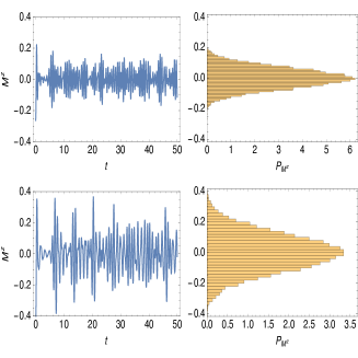
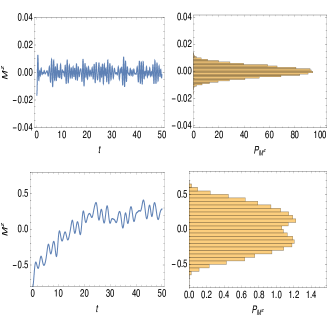
Nonetheless we have shown that indeed Gaussian equilibration is expected in two important cases: i) quasi-free Fermi systems where both the Hamiltonian and the observables are quadratic in Fermi operators, for any, non-critical, generic initial state [20] and, ii) small quench away from criticality[18, 32]. Since Gaussian equilibration is a rather weak form of equilibration, the result i) expresses in a precise and quantitative way the common folklore that integrability leads to a poorer (or no) equilibration. Likewise ii) can be explained noting that a small perturbation excites relatively few quasi-particles and therefore results in poor equilibration. In passing we note that Gaussian equilibration is not in contrast with the bound (1) in that quasi-free systems violate the non-resonant condition which leads to Eq. (1) while for a small quench, the initial state is not generic and $\mathrm{tr}\overline{\rho}^{2}\approx 1$ (in practice the constant $\alpha\to 0$ in the small quench limit).

Another class of probability distributions $P_{A}(a)$ arises for small quenches close to a quantum critical point, a scenario that will be described in more detail in Sec. 5. In this setting an even weaker form of equilibration takes place and the full time statistics $P_{A}(a)$ for a generic observable $A$, is predicted to have a universal bimodal shape.

These different forms of equilibration are illustrated by means of numerical simulations on the transverse field Ising model with next nearest neighbor interaction [see Sec. 4 and Eq. (8)] in Figure 1. In particular we performed the so called quantum quench numerical experiment: the system is initialized in the ground state of the Hamiltonian with parameters $h_{1},\,\kappa_{1}$. One then suddenly changes the parameters to $h_{2},\,\kappa_{2}$ and evolves the system with the resulting Hamiltonian. The observable considered is the total transverse magnetization $\mathsf{M}^{z}(t)=\sum_{j}\langle\sigma_{j}^{z}(t)\rangle$. In Fig. 1 we plot both the time series $\mathsf{M}^{z}(t)$ and its corresponding probability distribution $P_{\mathsf{M}^{z}}$. A large quench is a mean to initialize the system in a state which has little relation with the evolution Hamiltonian.

A large quench in a non-integrable model results in small fluctuations scaling as $\Delta\mathsf{M}^{z}\sim Le^{-\eta L}$ [from Eq. (1)]. However, if the system is quasi-free (and the observable is quadratic) the scaling becomes $\Delta\mathsf{M}^{z}\sim\sqrt{L}$, the Gaussian equilibration scenario discussed in Sec. 4. One has a Gaussian distribution also for a small quench performed in a gapped (non-critical) region of the phase diagram, with fluctuations scaling as $\Delta\mathsf{M}^{z}\sim\delta h\sqrt{L}$ ($\delta h$ quench amplitude). Finally, if the small quench is performed close to a quantum critical point, one obtains a bimodal distribution with large fluctuations scaling as $\Delta\mathsf{M}^{z}\sim\delta hL^{2\alpha}$ [$\alpha$ critical exponent, see Section 5]. For clarity these results are also summarized in Table 3.

Scaling of the (temporal) standard deviation $\Delta\mathsf{A}$ of an extensive observable for different scenarios. The asterisk refers to a quadratic observable. $V$ is the system’s volume, $L$ its linear size, $\delta\lambda$ the quench amplitude and the critical exponent $\alpha$ is defined in section 5. The corresponding theories will be developed in sections 4 and 5. Large quenches Small quenches Non-integrable       $\leq Ve^{-\eta V}$ Non-critical       $\delta\lambda\sqrt{V}$ Quasi-free^∗ $\sqrt{V}$ Quasi-critical $\delta\lambda L^{\alpha}$

4 Temporal fluctuations for quasi-free Fermi systems

We now consider a situation where both the Hamiltonian and the observable are quadratic in Fermi creation and annihilation operator. Note however that the initial state can be generic (i.e. not necessarily a Gaussian state). The Hamiltonian is $H=\sum_{x,y}c_{x}^{\dagger}M_{x,y}c_{y}=c^{\dagger}Mc$ (notation $c^{\dagger}=\left(c_{1}^{\dagger},\ldots,c_{V}^{\dagger}\right)$, $V$ number of sites), and the observable has the form $A=\sum_{x,y}c_{x}^{\dagger}a_{x,y}c_{y}=c^{\dagger}ac$. We will assume that $\left\|a\right\|=O\left(1\right)$ as this guarantees that the expectation values of $A$ scales at most extensively with the system volume . We assume here that both the Hamiltonian and the observable conserve particle number. The more general case can be obtained by performing a particle-hole transformation on some sites and considering a more general covariance matrix. Exploiting the quadratic nature of the problem and introducing the covariance matrix $R_{y,x}:=\mathrm{tr}\left(\rho_{0}c_{x}^{\dagger}c_{y}\right)$ ($0\leq R\leq\leavevmode{\rm 1\mkern-4.8muI}$) one can show that the expectation value $\mathsf{A}\left(t\right)$ reduces to a trace in the one-particle space:

$$\mathsf{A}\left(t\right)=\mathrm{tr}\left(ae^{-itM}Re^{itM}\right)\,.$$ (4)

Eq. (4) is perfectly analogous to its many-body version $\mathsf{A}\left(t\right)=\mathrm{tr}\left(Ae^{-itH}\rho_{0}e^{itH}\right)$ with $R$ playing the role of the initial state $\rho_{0}$. There is however one importance difference: while $\mathrm{tr}\rho_{0}=1$ one has $\mathrm{tr}R=N=\nu V$, i.e. is extensive (we defined $\nu=N/V$ the filling factor).

In the quasi-free setting the non-resonant condition necessary to prove Eq. (1), does not hold. Let us then seek for the analogous of the bound (1) in this quasi-free case. Let the one-particle Hamiltonian have the following diagonal form $M=\sum_{k}\Lambda_{k}|k\rangle\langle k|$. The time averaged covariance matrix is then $\overline{R}=\sum_{k}\langle k|R|k\rangle|k\rangle\langle k|$ (assuming non-degeneracy of the one-particle spectrum). We also define $F_{k,q}=\langle k|a|q\rangle\langle q|R|k\rangle$. Assuming the non-resonance condition for the one-particle spectrum, one gets $\Delta\mathsf{A}^{2}=\mathrm{tr}F^{2}-\sum_{k}\left(F_{k,k}\right)^{2}\leq\mathrm{tr}F^{2}=\sum_{k,q}\left|\langle k|a|q\rangle\right|^{2}\left|\langle q|R|k\rangle\right|^{2}$. Now $R$ is a non-negative operator and therefore it induces a (possibly degenerate) scalar product which satisfies Cauchy-Schwarz inequality: $\left|\langle q|R|k\rangle\right|^{2}=\left|\langle q|k\rangle_{R}\right|^{2}\leq\langle q|q\rangle_{R}\langle k|k\rangle_{R}=\langle q|R|q\rangle\langle k|R|k\rangle$. This leads us to

$$\Delta\mathsf{A}^{2}\leq\mathrm{tr}\left(a\overline{R}a\overline{R}\right)\leq\left\|a\right\|^{2}\mathrm{tr}\overline{R}^{2}.$$ (5)

Now, since $0\leq\overline{R}\leq\leavevmode{\rm 1\mkern-4.8muI}$, $\mathrm{tr}\overline{R}^{2}\leq\mathrm{tr}\overline{R}=\mathrm{tr}R=N$, we finally obtain $\Delta\mathsf{A}^{2}\leq\left\|a\right\|^{2}\nu V\,.$ This result seems to hint at the fact that fluctuations in the quasi-free setting are proportional to the system volume and are hence much larger than in the non-free case where they are exponentially small in $V$. For an extensive operator $A$ one has $\overline{\mathsf{A}}=O(V)$ and so the bound (5) translates into $\Delta\mathsf{A}/\overline{\mathsf{A}}\leq O(V^{-1/2})$. However Eq. (5) is just a bound and nothing prevents, in principle, to have much smaller fluctuations. In the following we will provide arguments justifying, in this quasi-free setting, extensivity for all the (temporal) cumulants.

Let us write again the generic expectation value (4) in the basis which diagonalizes $M$:

$$\mathsf{A}\left(t\right)=\overline{\mathsf{A}}+2\sum_{k<q}\left|F_{k,q}\right|\cos\left(t\left(\Lambda_{k}-\Lambda_{q}\right)+\phi_{k,q}\right)$$ (6)

with $\phi_{k,q}=\arg F_{k,q}$. Consider the moment generating function of $\mathsf{A}-\overline{\mathsf{A}}$ $\chi_{A}\left(\lambda\right):=\overline{e^{\lambda\left(\mathsf{A}\left(t\right)-\overline{\mathsf{A}}\right)}}$. The derivatives of $\chi_{A}$ at $\lambda=0$ are precisely the (centered) temporal moments of the random variable $\mathsf{A}(t)$. Now we observe that if the (one-particle) energies are rationally independent (i.e. linearly independent on the field of rationals), as a consequence of the theorem of the averages, infinite time averages are the same as uniform averages over the torus $\mathbb{T}^{V}$. In particular one has

$$\overline{e^{\lambda\left(\mathsf{A}\left(t\right)-\overline{\mathsf{A}}\right)}}=\left(\prod_{j=1}^{V}\int\frac{d\theta_{j}}{2\pi}\right)\exp{\left[\lambda E\left(\boldsymbol{\theta}\right)\right]}.$$ (7)

The generating function $\chi_{A}\left(\lambda\right)$ is exactly given by the partition function of the generalized, classical XY model with energy $E\left(\boldsymbol{\theta}\right)=2\sum_{k<q}\left|F_{k,q}\right|\cos\left(\theta_{k}-\theta_{q}+\phi_{k,q}\right)$ and inverse temperature $\beta=-\lambda$. The matrix $\left|F_{k,q}\right|$ defines the lattice of the interactions while the phases $\phi_{k,q}$ give the offset from which the angles are measured. Note that the behavior of the density $P_{A}\left(a\right)$ is dictated by $\chi_{A}\left(\lambda\right)$ in a neighborhood of $\lambda=0$ which corresponds to infinite temperature of the classical XY model.

Figure 2: Observation of Gaussian equilibration in quasi-free systems. Left panel: Ising model in transverse field. The observable is the transverse magnetization per site $m\left(t\right)=\langle\sigma_{i}^{z}\left(t\right)\rangle$. Right panel: tight-binding model withe twisted periodic boundary conditions. The observable is $A=\sum_{x=1}^{\ell}c_{x}^{\dagger}c_{x}$ where $\ell<L$ is only a fraction of the total system size $L$. The thick curves are the theoretical Gaussian prediction. Taken from Ref. campos_venuti_gaussian_2013.

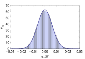
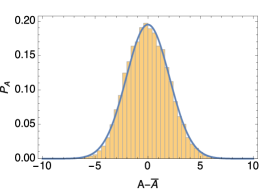
A similar mapping can also be obtained in the general (i.e. non quasi-free) case. However the one-particle space has a natural underlying geometric structure. For instance, the labels $k,q$ represent points in momentum (real) space in a superfluid (localized) phase and the distance $\left|k-q\right|$ is well defined. Now, when the matrix elements $\left|F_{k,q}\right|$ decay sufficiently fast as $\left|k-q\right|\to\infty$ the corresponding XY model is well defined in the thermodynamic limit, i.e. the intensive free energy has a limit as $L\to\infty$. This happens for instance in case $\left|F_{k,q}\right|$ decays exponentially in $\left|k-q\right|$ or if one has $\left|F_{k,q}\right|\sim 1/\left|k-q\right|^{\gamma}$ with $\gamma>D$. When this is the case one has $\chi_{A}\left(\lambda\right)=\exp L^{D}f\left(\lambda\right)$ where $f\left(\lambda\right)$ is the free energy per site. Moreover, under these conditions, one expects $f\left(\lambda\right)$ to be analytic in the high temperature, $\lambda=0$, limit, implying that all the cumulants of $\mathsf{A}\left(t\right)$ are extensive. From this we immediately draw the central limit theorem: as $L\to\infty$ the variable $(\mathsf{A}\left(t\right)-\overline{\mathsf{A}})/L^{D/2}$ tends in distribution to a Gaussian with zero mean and finite variance given by $\partial_{\lambda=0}^{2}f\left(\lambda\right)/2$. This situation has been referred to as Gaussian equilibration in Ref. campos_venuti_gaussian_2013. We would like to stress here that the term Gaussian equilibration refers to the situation where all the temporal cumulants of an extensive observable scale as the system’s volume. In this sense one cannot have Gaussian equilibration in the non-free setting since in that case the variance is exponentially small in the volume. However it is still possible that the properly rescaled variable $(\mathsf{A}\left(t\right)-\overline{\mathsf{A}})/\Delta\mathsf{A}$ , converges to a Gaussian in the infinite volume limit also for generic truly interacting systems.

The above arguments can be more precise for specific models and even transformed into theorems (see Ref. campos_venuti_gaussian_2013). A manifestation of Gaussian equilibration is shown in Fig. 2

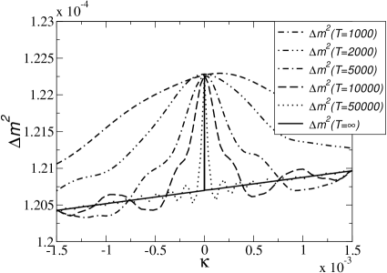
The above discussion shows that temporal fluctuations, and in particular the variance, can be used to detect proximity to an integrable point. Imagine a model which becomes integrable when an external parameter $\kappa$ becomes, say, zero. Since temporal variance is expected to be exponentially larger at an integrable point, it must be a discontinuous function of $\kappa$ at the integrable point. This predictions are confirmed by numerical simulations on the following model

$$H=-\sum_{i=1}^{L}\left[\sigma_{i}^{x}\sigma_{i+1}^{x}+h\sigma_{i}^{z}-\kappa\sigma_{i}^{x}\sigma_{i+2}^{x}\right]$$ (8)

which is non-integrable for all values $\kappa\neq 0$ (see Fig. 3).

Figure 3: Variance of $m\left(t\right)=\langle\sigma_{i}^{z}\left(t\right)\rangle$ for the model (8), as a function of the integrability breaking parameter $\kappa$. The quench parameters are $(\kappa_{0}=0,h_{0}=2.0),\,\to(\kappa_{1}=\kappa,\,h_{1}=2.7)$. The size is $L=8$. Dashed curves refers to the time variance computed with a finite observation window $[0,T]$.

5 Temporal fluctuations after a small quench

Another situation where the temporal fluctuations can be characterized in some generality is that of a small quench experiment. The system is prepared in the ground state of the Hamiltonian $H_{0}$ for $t<0$. At time $t=0$ one suddenly switches on a small perturbation $B$ such that the evolution Hamiltonian becomes $H=H_{0}+\delta\lambda B$, with $\delta\lambda$ a small parameter. The small quench condition can be found requiring that the exponentially small bound on the variance does not hold, i.e. $\mathrm{tr}(\overline{\rho}^{2})\nsim e^{-\alpha V}$. For small quench $\mathrm{tr}(\overline{\rho}^{2})$ can be related to the fidelity susceptibility $F$, more precisely one has $\mathrm{tr}(\overline{\rho}^{2})\simeq F^{4}$ [30]. The scaling behavior of the fidelity has been predicted in Ref. campos_venuti_quantum_2007. At regular point of the phase diagram, $F\sim\exp[-\alpha^{\prime}\delta\lambda^{2}V],$ whereas in the critical region the scaling becomes $F\sim\exp[-\alpha^{\prime\prime}\delta\lambda^{2}L^{2/\nu}]$, where $\nu$ is the correlation length critical exponent (defined by $\xi\sim|\lambda-\lambda_{c}|^{-\nu}$). Summarizing, the small quench condition reads $\delta\lambda\ll L^{-D/2}$ at regular points, or $\delta\lambda\ll L^{-1/\nu}$ if $H_{0}$ is at a critical point.

Finite size

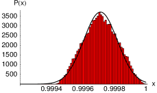
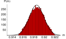
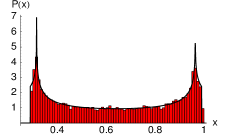
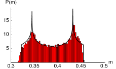
Let us now consider the full temporal statistic of $\mathsf{A}(t)$ at a fixed size and fixed –small– quench. The result for a generic observable is shown in Fig. 4. In the off-critical region, $\xi_{i/f}\ll L$ ($\xi_{i/f}$ denotes the correlation length of the initial/final Hamiltonian), full temporal statistics of generic observables are approximately Gaussian. In the complementary, quasi-critical region $\xi_{i/f}\gg L$, the distribution becomes bimodal characterized by larger variance. This result is completely general, it holds both for integrable and non-integrable models and generic observables[22, 18]. As can be seen from Fig. 4, this effect is significant even for small system sizes of the order of $L\sim 10$, and can be used to locate quantum critical points using out-of-equilibrium methods. This is an important point as it is notoriously difficult to observe precursor of quantum phase transitions with such short sizes using equilibrium indicators. The explanation of this phenomenon is the following. Consider the general form of an observable expectation value

$$\mathsf{A}(t)=\sum_{n,m}e^{-it(E_{n}-E_{m})}A_{m,n}\langle n|\psi_{0}\rangle\langle\psi_{0}|m\rangle.$$ (9)

Noting that, $\langle\psi_{0}|m\rangle=O(\delta\lambda)$ for $m>0$ and $\langle\psi_{0}|0\rangle=1+O(\delta\lambda^{2})$, in the small quench regime one has approximately

$$\mathsf{A}(t)\simeq\overline{\mathsf{A}}+\Big{[}\sum_{n>0}e^{-it(E_{n}-E_{0})}A_{0,n}\langle n|\psi_{0}\rangle+\mathrm{c.c.}\Big{]}.$$ (10)

If the energy gaps $(E_{n}-E_{0})$ are rationally independent one can show that the random variable $\mathsf{A}(t)$ in Eq. (10) is a sum of independent random variables: $\mathsf{A}(t)-\overline{\mathsf{A}}=\sum_{n>0}X_{n}$. Each $X_{n}$ has probability distribution function given by $1/(\pi\sqrt{\sigma_{n}^{2}-x^{2}})$ with variance $\sigma_{n}^{2}=2\left|A_{0,n}\langle n|\psi_{0}\rangle\right|^{2}$. If $H_{0}$ is at a regular point of the phase diagram, the coefficients $\langle n|\psi_{0}\rangle$ (and $A_{0,n}$) have no particular structure. Correspondingly one expects that none of them dominate and essentially $\mathsf{A}(t)$ will be Gaussian distributed. Note that, in this regime the total variance satisfies

$$\Delta\mathsf{A}^{2}=\sum_{n>0}\sigma_{n}^{2}\leq 2\sum_{n>0}A_{0,n}A_{n,0}=2[\langle A^{2}\rangle-\langle A\rangle^{2}].$$ (11)

The last term is precisely (twice) the quantum variance computed with state $|\psi_{0}\rangle$ (or $|0\rangle$ as they give the same result up to $O(\delta\lambda^{2})$). As such, for an extensive observable, the temporal variance is bounded by the volume $\Delta\mathsf{A}^{2}\leq O(V)$ in this regime.

The situation is different if $H_{0}$ (or $H$) is close to a quantum critical point. In this case one can show that $\langle E|\psi_{0}\rangle\sim\delta\lambda E^{-1/(\zeta\nu)}$ ($\zeta$ is the dynamical critical exponent) [18, 34]. At finite size, the lowest modes have energy, $E_{n}=v\left(2\pi n/L\right)^{\zeta}$ so that $\langle E_{n}|\psi_{0}\rangle\sim\delta\lambda L^{1/\nu}$. In practice, since in the region of validity of perturbation theory, $\langle E_{0}|\psi_{0}\rangle$ is already “large”, the sum rule $\sum_{n}\left|\langle E_{n}|\psi_{0}\rangle\right|^{2}=1$ constrains to have only very few $\langle E_{n}|\psi_{0}\rangle$ appreciably different from zero. In practice, a good approximation is obtained retaining only the two dominant terms in the sum in Eq. (10). Assuming for simplicity that $A_{0,n}\langle n|\psi_{0}\rangle$ are real, one has approximately, in the quasi-critical regime

$$\mathsf{A}(t)\simeq\overline{\mathsf{A}}+W_{1}\cos(t\omega_{1})+W_{2}\cos(t\omega_{2}),$$ (12)

with $W_{n}=2A_{0,n}\langle n|\psi_{0}\rangle$. The (temporal) probability density corresponding to Eq. (12) is precisely the density of states of a two dimensional, anisotropic, tight-binding model with hopping constants $W_{1},\,W_{2}$. It has been computed analytically in Ref. campos_venuti_unitary_2010. The resulting distribution $P_{A}(a)$ is symmetric around the mean $\overline{\mathsf{A}}$, supported in $\left[\overline{\mathsf{A}}-\left|\left|W_{1}\right|+\left|W_{2}\right|\right|,\overline{\mathsf{A}}+\left|\left|W_{1}\right|+\left|W_{2}\right|\right|\right]$ with logarithmic divergences at $a=\overline{\mathsf{A}}\pm\left|\left|W_{1}\right|-\left|W_{2}\right|\right|$ (see Fig. 4 lower panels).

Figure 4: Probability distributions for a small quench. $P\left(x\right)=\overline{\delta\left(x-\mathcal{L}\left(t\right)\right)}$ and $P\left(m\right)=\overline{\delta\left(m-\langle\sigma_{1}^{z}\left(t\right)\rangle\right)}$ refer to the Loschmidt echo (left panels) and magnetization respectively (right panels). Upper panels: the quench is performed at a regular point of the phase diagram. Lower panels: the same quench amplitude performed close to a quantum critical point. Note the much larger scale of the horizontal axis. The thick lines are our analytic predictions using only the three largest weights. The Hamiltonian is a non-integrable extension of the Ising model in transverse field. Sizes are $L=12(16)$ for the upper (lower) panel. See [18, 32] for details.

Thermodynamic limit

If one keeps the quench strength $\delta\lambda$ fixed, and increases the system size $L$, one will eventually enter the off-critical region. Increasing $L$ further one will leave the perturbative, small-quench, region and temporal variances will become exponentially small in the system size. Nevertheless one can wonder whether it is possible to obtain a meaningful limit, by keeping $\delta\lambda$ in the small quench region, and sending $L$ to infinity. This situation has been studied in Ref. campos_venuti_universal_2014.

Expanding $\mathsf{A}(t)$ up to first order in $\delta\lambda$ using Dyson expansion and the spectral resolution $H_{0}=\sum_{n}E_{n}|n\rangle\langle n|$, one gets

$$\mathsf{A}(t)=\overline{\mathsf{A}}+\delta\lambda\sum_{n>0}\left(Z_{n}e^{-it(E_{n}-E_{0})}+\mathrm{c.c.}\right)+O\left(\delta\lambda^{2}\right),$$ (13)

where the first, time-independent term is the average of $\mathsf{A}\left(t\right)$ and with $Z_{n}:=A_{0,n}B_{n,0}/\left(E_{n}-E_{0}\right)$ and the notation $A_{n,m}=\langle n|A|m\rangle$. The leading contribution to the temporal variance is therefore at second order and assuming that the gaps $E_{n}-E_{0}$ are non-degenerate one obtains

$$\Delta\mathsf{A}_{B}^{2}=2\delta\lambda^{2}\sum_{n>0}\left|Z_{n}\right|^{2}+O\left(\delta\lambda^{3}\right).$$ (14)

We added a subscript $B$ to recall that the variance is computed with perturbation $B$.

Using Eq. (13) we can actually obtain the full probability distribution of the variable $\mathsf{A}$. Assuming rational independence of the gaps $E_{n}-E_{0}$ and using the theorem of averages we obtain the following expression for the characteristic function of $\mathsf{A}$,

$$\overline{e^{is(\mathsf{A}-\overline{\mathsf{A}})/\delta\lambda}}=\prod_{n>0}J_{0}\left(2s\left|Z_{n}\right|\right):=J_{A}\left(s\right),$$ (15)

where $J_{0}$ is the Bessel function of the first kind. So the probability distribution of $\mathsf{A}$ is completely encoded in the characteristic function $J_{A}\left(s\right)$. The cumulants of the variable $(\mathsf{A}-\overline{\mathsf{A}})/\delta\lambda$ are given by $\kappa_{2p}=a_{2p}2^{2p}Q_{2p}$ with $Q_{2p}:=\sum_{n>0}\left|Z_{n}\right|^{2p}$ and known constants $a_{p}$ (odd cumulants are zero). Under the assumption of convergence the probability distribution of $\mathsf{A}$ is uniquely characterized by the coefficients $Q_{2p}$. Conversely the probability distribution uniquely defines the coefficients $Q_{2p}$ which are generalizations of the variance Eq. (14). Intuitively, at critical points the cumulants $\kappa_{2p}$ (through the coefficients $Q_{2p}$) may diverge with the system size.

Let us analyze the behavior of $Q_{2p}$ close to quantum criticality. In this case $\delta\lambda=\left|\lambda-\lambda_{c}\right|$ measures the distance from the critical point $\lambda_{c}$. Using standard scaling arguments one can show that $Q_{2p}\propto L^{2p\alpha}$ with $\alpha=2D+\zeta-\Delta_{A}-\Delta_{B}$ (see Ref. campos_venuti_universal_2014 for details). Here $\Delta_{A/B}$ are the scaling dimensions of the observables $A/B$ that we assumed extensive. Instead, away from criticality the expectation is $Q_{2p}\propto L^{D}$. Requiring that, at finite size, $Q_{2p}$ is analytic in the system parameters and matches the above scaling, one can predict the behavior of $Q_{2p}$ close to the critical point both in the critical region $\xi\gg L$ and in the off-critical one $\xi\ll L$ :

$$\kappa_{2p}\propto Q_{2p}\sim\begin{cases}L^{2\alpha p}&\xi\gg L\\ \delta\lambda^{D\nu-2\alpha p\nu}L^{D}&\xi\ll L\end{cases}\,.$$ (16)

As usual in finite size scaling theory, the above prediction refers to the singular part of $Q_{2p}$, on top of which there is always a regular, extensive, contribution [35].

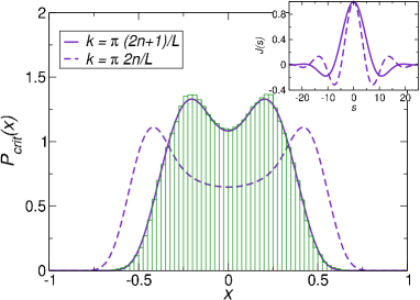
Consider now the rescaled random variable $\mathsf{X}\left(t\right)=(\mathsf{A}\left(t\right)-\overline{\mathsf{A}})/\Delta\mathsf{A}$ whose cumulants are given by $\kappa_{2n}^{X}=\kappa_{2n}^{A}/(\kappa_{2}^{A})^{n}$ for $n\geq 1$ whereas odd cumulants are zero. The probability distribution of $\mathsf{X}$ is uniquely determined by the ratios $R_{2p}=Q_{2p}/\left(Q_{2}\right)^{p}$. From Eq. (16) we see that in the quasi-critical regime, these ratios are scale independent and define some presumably universal constants. Let us now find these constants. With the help of density of states $\rho\left(E\right)=\mathrm{tr}\left(\delta\left(H-E\right)\right)$ we can write $Q_{p}=\int Q_{p}\left(E\right)\rho\left(E\right)dE$. Since $\rho\left(E\right)dE$ is scale invariant, from $Q_{p}\propto L^{p\alpha}$ we derive $Q_{p}\left(E\right)\propto E^{-p\alpha/\zeta}$. We now assume that at the critical point one has vanishing energy excitations with definite momentum. In order to proceed further we must specify the form of the low energy dispersion. The simplest possibility is a rotationally invariant spectrum at small momentum, i.e. $E\simeq C\left\|\boldsymbol{k}\right\|^{\zeta}=C(\sum_{j}k_{j}^{2})^{\zeta/2}$ where $\boldsymbol{k}$ is a quasi-momentum vector. In one dimension this is essentially the only possibility but for $d>1$ one can also have anisotropic transitions where the form of the dispersion depends on the direction. Using the isotropic assumption we obtain $Q_{p}\simeq C^{\prime}\sum_{\boldsymbol{k}}\left\|\boldsymbol{k}\right\|^{-p\alpha}.$ In doing so we have essentially restricted the sum over $n$ to the one-particle contribution. This is expected to be the leading contribution whereas higher particle sectors contribute at most to the extensive, regular term [36]. This shows that the cumulants of $\mathsf{X}$ are uniquely specified by the critical exponent $\alpha$ and the boundary conditions that specify $\boldsymbol{k}$. More precisely the probability distribution of the rescaled variable $\mathsf{X}\left(t\right)$ is a universal function which depends only on $\alpha$ and the boundary conditions. A related universal behavior has been observed in [37, 38] in the case of the sine-Gordon model. Let us assume for concreteness that the lattice is a hyper-cube of size $L$ and the boundary conditions (BC) are such that moments are quantized according to $\boldsymbol{k}=(2\pi/L)(\boldsymbol{n}+\boldsymbol{b})$ with $n_{i}=1,\ldots,L$. The BC on the direction $i$ are fixed by $b_{i}\in\left[0,1/2\right]$ which interpolates between periodic (PBC, $b_{i}=0$) and anti-periodic (ABC, $b_{i}=1/2$) BC. In the infinite volume limit the ratios $R_{2p}=Q_{2p}/\left(Q_{2}\right)^{p}$ become universal quantities that can be explicitly computed (see [19]). The result is

$$\lim_{L\to\infty}R_{2p}=\begin{cases}\delta_{p,1}&2\alpha\leq D\\ \zeta_{\boldsymbol{b}}\left(2p\alpha\right)/\zeta_{\boldsymbol{b}}\left(2\alpha\right)^{p}&2\alpha>D.\end{cases}$$ (17)

where $\zeta_{\boldsymbol{b}}\left(\alpha\right)=\sum_{n_{1}=1}^{\infty}\cdots\sum_{n_{d}=1}^{\infty}\left\|\boldsymbol{n}+\boldsymbol{b}\right\|^{-\alpha}$ denotes a generalized $D$-dimensional Hurwitz-Epstein $\zeta$-function. For $2\alpha\leq D$ the characteristic function of $\mathsf{X}(t)$ becomes $e^{-s^{2}/2}$ in the thermodynamic limit and so $\mathsf{X}$ tends in distribution to Gaussian. Clearly the Gaussian behavior observed here for not sufficiently relevant operators, i.e. $\alpha\leq D/2$, is also to be expected at regular points of the phase diagram. These predictions have been checked for the XY model in transverse field[19]. Considering the transverse magnetization $\mathsf{M}\left(t\right)=\sum_{j}\langle\sigma_{j}^{z}(t)\rangle$ as observable, its temporal characteristic function can be computed analytically. The scaling dimensions in this case are $D=\zeta=\Delta_{A}=\Delta_{B}=1$ implying $\alpha=1$. One can then prove analytically that in the limit $L\to\infty$, Eq. (15) becomes $\prod_{n=0}^{\infty}J_{0}(\lambda/\alpha_{n})$ with $\alpha_{n}=\sqrt{\zeta_{1/2}\left(2\right)/2}\,(n+1/2)$. This in turns implies Eq. (17) with $\alpha=1$ and $b=1/2$ as predicted. A numerical demonstration is provided in Fig. 5. A discussion of the regular points as well as a comparison of the dynamical central limit type theorem here discussed and the one for quantum fluctuations at equilibrium can be found in Ref. campos_venuti_universal_2014.

Figure 5: Critical probability distribution for the transverse magnetization $[\langle M(t)\rangle-\overline{M}]/(L\delta h)$ in the XY-model in transverse field. The inset shows the characteristic function, which in the thermodynamics limit becomes $J\left(s\right)=\prod_{n=0}^{\infty}J_{0}\left(s/\left(2n+1\right)\right)$. The histogram is computed performing a numerical experiment on the Ising model on a chain of $L=1006$ sites with periodic boundary conditions corresponding to quasimomenta of the form $k=\pi(2n+1)/L$. The continuous (dashed) lines refer to quasimomenta of the form $k=\pi(2n+1)/L$ ($k=2\pi n/L$). The quench parameters are $h_{1}=1$, $h_{2}=1.0003$ and $\gamma_{1}=\gamma_{2}=1$. The statistics is obtained sampling 600,000 random times uniformly distributed in $\left[0,T\right]$ with $T=600,000$. The distribution is unchanged using a different $\gamma_{1}=\gamma_{2}\neq 0$ as implied by universality. From [19].

6 Temporal Fluctuations in non-homogeneous systems

The results of the previous section, valid for homogeneous systems, indicate that the temporal fluctuations can be used as indicator of quantum criticality. A by-product of Eq. (16) is that, for a small quench (in the sense of Section 5), the temporal fluctuations diverge as $\Delta\mathsf{A}_{B}^{2}\sim L^{2\alpha}$ in the quasi-critical region $\xi\gg L$. The recipe to estimate critical points is standard (see e.g. [35, 39]). Since in the off-critical region $L\gg\xi$, $\Delta\mathsf{A}_{B}^{2}$ is extensive (for extensive observable $A$ and perturbation $B$), finite size pseudo critical point $g^{\ast}(L)$ can be defined as the location of the maximum of $\Delta\mathsf{A}_{B}^{2}$, as a function of the tunable parameter $g$. The sequence $g^{\ast}(L)$ converges to the exact critical point as $L\to\infty$. For this procedure to succeed one must be able to identify a maximum, i.e. one needs $2\alpha>D$. We can now compare the ability of the the temporal variance to act as indicator of quantum criticality with that of other standard, equilibrium, indicators such as quantum fluctuations $\Delta A^{2}:=\langle A^{2}\rangle-\langle A\rangle^{2}$, or the generalized susceptibility $\chi_{AB}:=\left.\partial_{\lambda}\langle A\rangle_{\lambda}\right|_{\lambda=0}$, (here $\langle\bullet\rangle_{\lambda}$ indicates the quantum average taken with the ground state of $H(\lambda)=H_{0}-\lambda B$). Standard scaling arguments allow to show that $\Delta A^{2}\sim L^{2d-2\Delta_{A}}$, whereas $\chi_{AB}\sim L^{\alpha}$. Since all quantities are extensive in the off-critical region, pseudo critical points can be defined when $\Delta_{A}<D/2$ using quantum fluctuations, and for $\alpha>D$ in case of the susceptibility. Taking for simplicity $A=B$, pseudo-critical points can be defined provided $\Delta_{A}<D/2$ (using quantum fluctuations), $\Delta_{A}<D/2+\zeta/2$ (using generalized susceptibilities), $\Delta_{A}<(3/4)D+\zeta/2$ (using temporal variances). Since the smaller $\Delta_{A}$, the more relevant is the operator $A$, we see that the above conditions are less and less restrictive. In other words more quantum phase transitions can be observed and located resorting to the temporal variance.

The above considerations suggest that temporal variances may also be used to detect phase boundaries between different phases in spatially inhomogeneous systems. Suppose a large system can be divided in two neighboring regions A and B, and that the system is in phase $P_{A}$ in region A and in phase $P_{B}$ in region B. For simplicity one can think that the system is a very long one-dimensional chain, and regions A, B, are two segments separated by a boundary region C. Since the state of phase $P_{A}$ cannot be deformed continuously into the state in B preserving the symmetries of the model, one expects that some pseudo-critical behavior emerges in the boundary region separating region A form region B. A particularly interesting example of such inhomogeneous systems is provided by optical lattice experiments where the presence of a (to a good approximation) harmonic confining potential breaks translation invariance. Experiments [40, 41, 42] have been able to resolve the site-occupation profiles and reveal the characteristic “wedding cake” structure in which Mott plateaus are flanked by superfluid domains. For the purpose of accurately determining the boundaries between those domains, several local, equilibrium, compressibilities have been proposed in the literature [43, 44, 45, 46], including $\kappa_{i}:=\partial\langle\hat{n}_{i}\rangle/\partial\mu_{i}$ [43], as well as the site-occupation fluctuations $\Delta n_{i}^{2}:=\langle\hat{n}_{i}^{2}\rangle-\langle\hat{n}_{i}\rangle^{2}$ [45, 46], where $\langle\bullet\rangle$ stands for the quantum expectation value and $\mu_{i}$ is the local chemical potential at site $i$. In Ref. yeshwanth_small_2014 extensive numerical simulations confirmed that temporal fluctuations of the site-occupation can serve as efficient detectors of this local quantum criticality [45] (see also [48]), and in fact reveals details which cannot be observed using the equilibrium local compressibility $\kappa_{i}$. We now briefly review those findings.

We first consider a class of hard-core boson models, which can be mapped to systems of interacting Fermions after Jordan-Wigner transformation. This allows to perform numerical simulations on long chains and so to obtain proper scaling of quantities with the system size $L$. The Hamiltonian is given by

$$\hat{H}_{0}=-J\sum_{i=1}^{L-1}(\hat{b}_{i}^{\dagger}\hat{b}_{i+1}+\mathrm{h.c.})+\sum_{i=1}^{L}[\lambda g_{i}\hat{n}_{i}+V_{0}(-1)^{i}\hat{n}_{i}].$$ (18)

which can be thought of as the limit $U/J\rightarrow\infty$ of the Bose-Hubbard model [49]. In Eq. (18), $\hat{b}_{i}^{\dagger}$ ($\hat{b}_{i}$) is the creation (annihilation) operator of a hard-core boson at site $i$, $\hat{n}_{i}=\hat{b}_{i}^{\dagger}\hat{b}_{i}$, and $g_{i}$ describes a harmonic confining potential, with $g_{i}=L^{-2}(i-L/2+\epsilon)^{2}$. The trap is shifted off-center by a small amount $\epsilon$ to remove degeneracies in the energy levels and gaps of the Hamiltonian [see the discussion of Eq. (19)]. We initialize the system in a ground state $|\Psi(0)\rangle$ of a lattice with $L$ sites and $N$ hard-core bosons. After performing a sudden quench on the trap potential, $\lambda\rightarrow\lambda+\delta\lambda$ at time $t=0$, the system evolves unitarily as $|\Psi(t)\rangle=\exp(-i\hat{H}t)|\Psi(0)\rangle$. The post-quench Hamiltonian is given by $\hat{H}=\hat{H}_{0}+\delta\lambda\,\hat{B}$. A Jordan-Wigner transformation maps Eq. (18) onto a Hamiltonian quadratic in fermion operators $\hat{f}_{i}^{\dagger}$ and $\hat{f}_{i}$. From that transformation, it follows that the site occupations of hard-core bosons and spinless fermions are identical, i.e. $\hat{n}_{i}=\hat{b}_{i}^{\dagger}\hat{b}_{i}=\hat{f}_{i}^{\dagger}\hat{f}_{i}$. The fermionic Hamiltonian can be written as $\hat{H}=\sum_{i,j}\hat{f}_{i}^{\dagger}M_{i,j}\hat{f}_{j}$ with $M_{i,j}=-J(\delta_{i,j+1}+\delta_{i,j-1})+\left[(\lambda+\delta\lambda)g_{i}+V_{0}(-1)^{i}\right]\delta_{i,j}$. The noninteracting character of the fermionic system allows one to write temporal fluctuations of site occupations (and in fact of any quadratic observable in the fermions) in terms of one-particle quantities alone. Consider a general quadratic observable of the form $\hat{X}=\sum_{i,j}\hat{f}_{i}^{\dagger}\Gamma_{i,j}\hat{f}_{j}$. One can show that $\mathsf{X}(t)=\langle\Psi(t)|\hat{X}|\Psi(t)\rangle=\mathrm{tr}(\hat{X}e^{-it\hat{H}^{\prime}}\rho_{0}e^{it\hat{H}^{\prime}})=\mathrm{tr}(\Gamma e^{-itM}Re^{itM})$ where $R$ is the covariance matrix of the initial state $\rho_{0},$ i.e., $R_{i,j}=\mathrm{tr}(\rho_{0}\hat{f}_{j}^{\dagger}\hat{f}_{i})$ (note that the initial state does not necessarily need to be Gaussian). Let the one-particle Hamiltonian $M$ have the spectral representation $M=\sum_{k}\Lambda_{k}|k\rangle\langle k|$ ($|k\rangle$ are one the particle eigenfunctions) and define $F_{k,q}=\langle k|\Gamma|q\rangle\langle q|R|k\rangle$ where $\Gamma,\,R$ are one-particle operators. The temporal variance of $\mathsf{X}$ is given by

$$\Delta\mathsf{X}^{2}=\mathrm{tr}(F^{2})-\sum_{k}(F_{k,k})^{2}.$$ (19)

Equation (19) relies on the assumption of the non-resonant conditions for the one-particle spectrum [5, 20], which has been verified in our numerical calculations (for $\epsilon\neq 0$). To compute the variance of the site occupations we simply take $X=n_{i}$ which implies $\Gamma_{x,y}^{(i)}=\delta_{i,x}\delta_{i,y}$.

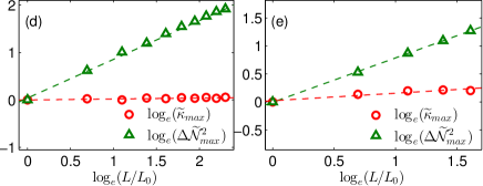
For $V_{0}=0$ results of typical simulations are shown in Fig. (6) panels a), b). In this case the state in the trap center is approximately the completely filled state $|1,1,\ldots,1,1\rangle$, whereas at the boundary it is essentially the empty state $|0,0,\ldots,0,0\rangle$. Clearly both the density fluctuations $\Delta n_{i}^{2}$ and the local compressibility are able to distinguish the two phases. Both quantities are approximately constant and non-zero only in the interface region [Fig. (6) panels a), b)]. Instead the temporal fluctuations of the site occupation $\Delta\mathsf{n}_{i}^{2}$ show strong fluctuations in the interface region. A closer look at the density profile in the interface region [Fig. (6) panel b)] reveals that the density evolves in a stepwise fashion. Small subregions of constant density are intertwined with pseudo-critical regions which are properly spotted by the presence of a large temporal variance. The local compressibility instead is hardly able to resolve such fine details. Moreover the maxima of the temporal variance diverge much more rapidly than those of the compressibility. A scaling analysis reveals that both quantities follow a power law with the following exponents: $\Delta\mathsf{n}_{\mathrm{max}}^{2}\propto L^{0.83}$, whereas for the compressibility one finds $\kappa_{\mathrm{max}}\propto L^{0.05}$. This means that the temporal variance provides a stronger signal as opposed to the local compressibility.

Similar results are observed in presence of a nonzero staggerization. The only caveat is that for $V_{0}\neq 0$ one must consider a unit cell consisting of two neighboring sites [see Fig. (6) panel c)]. In the trap center the state is approximately $|1,0,1\ldots,1,0\rangle$ separated by an approximately empty state at the boundaries. Once again both the temporal variance and the local compressibility are able to distinguish the phases. The finite-size scaling of the maximum of both quantities, reveals that $\Delta\mathsf{n}_{\mathrm{max}}^{2}\propto L^{0.80}$ and $\kappa_{\mathrm{max}}\propto L^{0.14}$ [see Fig. 6(e)], respectively, meaning that the temporal variance offers better detectability.

Figure 6: (a) “Wedding cake” site occupation profile of hard-core bosons in a one-dimensional harmonic trap described by Eq. (18) with $V_{0}=0$. The system consists of $L=500$ sites and $N=250$. The Hamiltonian parameters are $\lambda=10$, $\epsilon=0.2$, $\delta\lambda=L^{-2}$ ($J=1$ throughout). The phase boundaries between the Mott plateau located at the trap center and the adjacent superfluid regions can be detected by the conventional local compressibility $\kappa_{i}$ (red) and by the temporal variance of the site occupations $\Delta\mathsf{n}_{i}^{2}$ (green) introduced in this work. (b) A closer look at the superfluid region for the system shown in (a) reveals temporal variance peaks at the interface between the superfluid and the Mott insulator. (c) Unit cell average site occupancy in the presence of a staggered potential Eq. (18). This is a system with $L=500$, $N=150$, and parameters $\lambda=10$, $\epsilon=0.2$, $\delta\lambda=1/L^{2}$, $V_{0}=1.5$. (d) and (e) Finite-size scaling of the maximum temporal variance of the site occupations and of the compressibility vs $L$. We find $\Delta\mathsf{n}_{\mathrm{max}}^{2}\propto L^{0.83}$ and $\kappa_{\mathrm{max}}\propto L^{0.05}$ for $V_{0}=0$ (e) and and $\Delta\mathsf{n}_{\mathrm{max}}^{2}\propto L^{0.80}$ and $\kappa_{\mathrm{max}}\propto L^{0.14}$ for $V_{0}=1.5$. All quantities in the plots are made dimensionless by dividing by their values when $L_{0}=50$, i.e., $\widetilde{\kappa}_{\mathrm{max}}=\kappa_{\mathrm{max}}(L)/\kappa_{\mathrm{max}}(L_{0})$ and $\Delta\widetilde{\mathsf{n}}_{\mathrm{max}}^{2}=\Delta\mathsf{n}_{\mathrm{max}}^{2}(L)/\Delta\mathsf{n}_{\mathrm{max}}^{2}(L_{0})$. From [47].

The proposed approached is clearly not limited to integrable models. We then considered a system consisting of hard-core bosons with nearest and next-nearest interactions (a $J$-$V$-$V^{\prime}$ model) in the presence of a harmonic trap, described by the Hamiltonian

$$\hat{H} =\sum_{i=1}^{L-1}\left[-J(\hat{b}_{i}^{\dagger}\hat{b}_{i+1}+\mathrm{h.c.})+V\left(\hat{n}_{i}-\frac{1}{2}\right)\left(\hat{n}_{i+1}-\frac{1}{2}\right)\right.$$

$$\left.+V^{\prime}\left(\hat{n}_{i}-\frac{1}{2}\right)\left(\hat{n}_{i+2}-\frac{1}{2}\right)\right]+\lambda\sum_{i=1}^{L}i^{2}\hat{n}_{i}.$$ (20)

Note that, in order to maximize the size of insulating and superfluid domains, only one half of what would be the harmonic trap is considered in Eq. (20).

In the absence of a trap, the phase diagram of Hamiltonian (20) has been studied using the density matrix renormalization group technique [50]. The competition between nearest-neighbor and next-nearest-neighbor interactions generates four phases: two charge-density-wave insulator phases, a superfluid (Luttinger-liquid) phase, and a bond-ordered phase. In the presence of a trap, and for a suitable choice of the parameters, the same four phases can be observed. We focus our analysis on a parameter regime where the system exhibits a charge density wave of type one (CDW-I) in the center of the trap, which is surrounded by a superfluid phase. In this CDW-I phase the state is approximately $|1,0,1\ldots,1,0\rangle$ as we have seen previously for model (18) with $V_{0}\neq 0$. However the CDW-I phase here is not due to the presence of a translationally symmetry breaking term $V_{0}$ but is stabilized by the presence of interactions. There are two other phases that have larger unit cells, consisting of 4 sites for CDW-II and 3 sites for bond-order. The CDW-I phase is the best suited for our purposes because we are able to observe several unit cells that exhibit its expected properties.

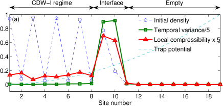
In Fig. 7(a), we show results for a site-occupation profile exhibiting a CDW-I plateau surrounded by a small superfluid domain. In the same figure one can see that, at the edge of the CDW-I plateau, the local compressibility $\kappa_{i}$ exhibits a much weaker signal than the temporal fluctuations $\Delta\mathsf{n}_{i}^{2}$. (Note that we used multiplicative factors to enhance $\kappa_{i}$ and reduce $\Delta\mathsf{n}_{i}^{2}$ so that both measures can appear on the same scale). Also, notice that $\kappa_{i}$ does not vanish in the CDW-I plateau, which exhibits nonzero site occupation fluctuations. Since calculations for larger systems are prohibitively large, a finite-size scaling analysis of the observables is not possible here. Nonetheless, from Fig. 7(a), it is evident that the temporal variance is a better indicator of the interface between domains than the local compressibility. In fact, compared to the integrable systems considered in the preceding section, the advantage of using $\Delta\mathcal{N}_{i}^{2}$ over $\kappa_{i}$ to identify interfaces between domains is enhanced, especially taking into account the small system sizes considered here.

Figure 7: Spatial profile of the temporal variance of the site occupations $\Delta\mathsf{n}_{i}^{2}$ and of the local compressibility $\kappa_{i}$ for the model in Eq. (20). We initialize the system with 19 sites and 5 particles in the ground state with parameters $J=1$, $V=8.0$, $V^{\prime}=0.5$ and $\lambda=0.1225$. The quench is performed by changing the trap potential from $\lambda$ to $\lambda+\delta\lambda$ with $\delta\lambda=0.0061$. From [47].

Figure 8: (a) Distributions of the site occupations $\mathsf{n}_{i}(t)$ at sites near the interface between the CDW-I and the superfluid phase. The quench amplitude $\delta\lambda$ is the same as for Fig. 7. (b) and (d) Distribution function of the site occupation at a site deep in the CDW-I regime (site $i=1$) and at a site at the edge of the CDW-I domain (site $i=10$), respectively. (c) and (e) Time dependence of $\mathsf{n}_{i}(t)$ corresponding to (b) and (d), respectively. The data are obtained by sampling each $\mathsf{n}_{i}(t)$ at $N=4\times 10^{4}$ random times uniformly distributed in $\left[0,T\right]$ with $T=40\hbar/J$. From [47].

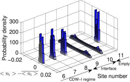
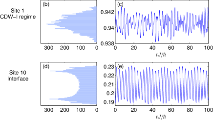
One can also go beyond the second moment analysis presented so far and examine the full probability distribution $P_{i}(x)$ of the random variable $\mathsf{n}_{i}(t)$ equipped with the time average measure $\overline{\bullet}$. Based on the results for homogeneous systems [18, 19], we expect $P_{i}(x)$ to be a single peaked, approximately Gaussian, narrow distribution for sites $i$ deep in the (gapped) insulating regime. On the contrary, $P_{i}(x)$ is predicted to be a double peaked distribution with a relatively large variance for (critical) interface sites $i$. In a limiting, somewhat simplified case, $P_{i}(x)$ can be approximated by a two parameter distribution $P_{i}(x)=1/\left(\pi\sqrt{2\Delta\mathsf{n}_{i}^{2}-(x-\overline{\mathsf{n}_{i}})^{2}}\right)$ [18].

In Fig. 8(a), we show the distribution $P_{i}(x)$ for sites near the interface separating the insulating and superfluid regions. For sites $i$ deep in the insulating region [Fig. 8(b)], the site occupations fluctuate about one unique central value, resulting in a singly-peaked distribution function. This signifies measure concentration, indicating local equilibration in the finite system considered here [Fig. 8(c)]. In contrast, as one moves closer to the interface [Fig. 8(d)], the distribution starts developing two peaks corresponding to a bistability characteristic of phase boundaries. This breakdown of measure concentration indicates the breakdown of local equilibration [Fig. 8(e)] and can thus be used as a witness for spatial phase separation.

7 The measurement problem

So far the analysis has been mostly theoretical. We will now try to address a bit more concretely the problem of determining the temporal fluctuations $\Delta\mathsf{A}^{2}$ from experimental data.

So far we assumed, quite naturally, that we can determine, for various times $t_{j}$, the expectation value $\mathsf{A}(t_{j})=\langle A(t_{j})\rangle$ exactly. This requires to prepare the system many times with the same initial state and perform say, $N_{s}$ measurements at the same time $t_{j}$ to obtain the $\mathsf{A}(t_{j})$ with sufficient precision (in principle $N_{s}$ may depend on $j$ but we won’t need this generalization here). Moreover the process will be repeated $N_{d}$ times at different times, to obtain $\mathsf{A}(t_{1}),\ldots,\mathsf{A}(t_{N_{d}})$. Since typically the variables are compactly supported (i.e. $\langle A(t_{j})\rangle$ takes values in a compact set), one can use the Chernoff bound to deduce that the empirical mean converge to the actual mean exponentially fast in the number of measurement $N_{s}$. For example, consider the case where $A$ is a Fermionic number operator at site $i$: $A=c_{i}^{\dagger}c_{i}$. Denote with $X_{n}$ the result of the $n$-th measurement of $A$ (always after the same preparation time $t_{j}$). In this case $X_{n}$ are Bernoulli trials (i.e. $X_{n}$ takes only two values, 0,1). Denoting the empirical mean with $Z_{N_{s}}=N_{s}^{-1}\sum_{n=1}^{N_{s}}X_{n}$ and calling $\mu=\mathsf{E}[Z_{N_{s}}]$ ($\mathsf{E}[\bullet]$ denotes the expectation value), the Chernoff’s bound states that, for $\delta\in(0,1]$,

$$\mathrm{Prob}\left(Z_{N_{s}}<(1-\delta)\mu\right)\leq e^{-N_{s}\delta^{2}/2},$$ (21)

(a similar inequality exist to bound $Z_{N_{s}}$ from below). In other words, the error one does in estimating $\mu$ is exponentially small in the number of measurements $N_{s}$. However this may not be the best strategy to obtain the temporal variance $\Delta\mathsf{A}^{2}$. In order to design better strategies we must look deeper into the measurement problem in our out-of-equilibrium setting (the system is prepared in state $\rho_{0}$ at time $t=0$ and let evolve unitarily thereafter). Let us indicate with $X_{j}^{n}$ the result of the $n$-th measurement of $A$ performed at time $t_{j}$. Differently from the equilibrium case, the variables $X_{j}^{n}$ at different times, are still independent but are not identically distributed. In the language of statistics what we would like to build is a consistent estimator of the temporal variance $\Delta\mathsf{A}^{2}$. A consistent estimator is a method to obtain a given quantity with the property that, as the number of data point increases, the estimator converges in probability to the actual parameter we are trying to estimate. In our case the data points are the variables $X_{j}^{n}$. We now show that it is possible to estimate $\Delta\mathsf{A}^{2}$ taking $N_{s}$ as small as $2$. Suppose that we perform two measurements of $A$ at the same time $t_{j}$, which we denote with $A_{j}^{1},A_{j}^{2}$. The label $j$ runs form $1$ to $N_{d}$, and we are performing a total of $N_{s}N_{d}=2N_{d}$ measurements. The following quantity can be shown to be a consistent estimator of $\Delta\mathsf{A}^{2}$:

$$s_{2}=\frac{1}{N_{d}}\sum_{j=1}^{N_{d}}A_{j}^{1}A_{j}^{2}-\frac{1}{N_{d}^{2}}\sum_{i,j}A_{i}^{1}A_{j}^{2}.$$ (22)

Indeed, taking the expectation value, one obtains

$$\mathsf{E}[s_{2}]=\frac{1}{N_{d}}\sum_{j=1}^{N_{d}}\langle A(t_{j})\rangle^{2}-\Big{(}\frac{1}{N_{d}}\sum_{j=1}^{N_{d}}\langle A(t_{j})\rangle\Big{)}^{2}.$$ (23)

Sampling $t_{j}$ uniformly in $[0,T]$ the above quantity converges to $\Delta\mathsf{A}^{2}$ as $N_{d}\to\infty$. Alternatively, denoting with $\mathsf{T}$ the uniform time average over all the different times $t_{j}$, one has $\mathsf{T}[\mathsf{E}[s_{2}]]=\Delta\mathsf{A}^{2}+O\left(N_{d}^{-1}\right)$, i.e. $s_{2}$ is unbiased up to an error $O\left(N_{d}^{-1}\right)$. Similarly one can show that $\mathrm{\mathsf{var}}[s_{2}]=O\left(N_{d}^{-1}\right)$, implying the consistency of $s_{2}$.

In order to minimize the experimental cost, it would be important to find the most efficient estimators $S(\Delta\mathsf{A}^{2})$ for the temporal variance. An estimator is efficient if it is unbiased and if the Cramer-Rao bound [51], $\mathrm{\mathsf{var}}[S(\Delta\mathsf{A}^{2})]\geq 1/I_{\Delta\mathsf{A}^{2}}$ ($I_{\Delta\mathsf{A}^{2}}$ is the Fisher information) is attained. Clearly further investigations are necessary in this direction, but these preliminary results indicate that the analysis of the temporal variance may be an efficient tool to characterize critical properties with unprecedented details.

8 Conclusions

In this review we have described some basic properties of the temporal fluctuations in isolated, out-of-equilibrium systems. In this setting a quantum system is initialized in a given state and then let evolve unitarily undisturbed thereafter. As a consequence, quantum expectation values of observables become oscillating functions. A great deal of physical properties are encoded in such temporal fluctuations. In the general case temporal fluctuations of physical observables are exponentially small in the system volume. This is encouraging as it allows to define an average, equilibrium state, with exponential accuracy. This result is however violated in a few important cases. First of all, this result does not hold for integrable (quasi-free) systems. In integrable systems, instead, temporal fluctuations are exponentially larger and scale with the system’s volume. This allows to use temporal fluctuations to study proximity to integrable points. Temporal fluctuations can also be completely characterized in a small quench experiment. In this setting the system is initialized in the ground state of a given Hamiltonian and then driven out-of-equilibrium by applying a sudden, small perturbation. Temporal fluctuations can then be used to characterize the underlying, unperturbed system. If the unperturbed system is at a regular point of the phase diagram, temporal fluctuations of generic extensive observables become Gaussian. On the contrary, close to a quantum critical point, temporal fluctuations acquire a universal bistable distribution which depends on a single critical exponent. The results presented here, indicate that temporal fluctuations may be used in experiments as a tool for probing criticality or integrability of isolated quantum systems.

What has been left out? The theory of temporal fluctuations presented in this review parallels, in a way, the theory of quantum fluctuations of systems at equilibrium [52]. In that case one knows that distributions of general observables are Gaussian, universal, bimodal, for gapped, critical, and symmetry broken phases respectively. In a similar fashion we have been able to single out distinctive regimes where the general form of the temporal distribution can be predicted and the size of the fluctuations estimated. Several aspects deserve future investigations on the hand of this analogy. First of all one may ask if other distributions exist in particular regimes. Furthermore, one may consider temporal autocorrelation functions of observables $\psi(s)=\overline{\mathsf{A}(t)\mathsf{A}(t+s)}$ which are the analog of the correlations function of equilibrium statistical mechanics. What kind of informations can be obtained from its study? More generally, what properties of the asymptotic equilibrium state ρ can be inferred from the study of temporal fluctuations? This dynamical setting has much more freedom and complexity than the equilibrium case and therefore new questions arise. For example, one may ask how does the equilibration pattern change for slow as opposed to sudden quenches or what is the effect of quenching from one phase to another one. The use of temporal fluctuations as a, conceptual as well as practical, tool has just started to be investigated.

References

- [1] S. Lloyd, ph.D., The Rockfeller University1988.
- [2] S. Goldstein, J. L. Lebowitz, R. Tumulka and N. Zanghì, Canonical Typicality, Phys. Rev. Lett. 96, p. 050403 (February 2006).
- [3] S. Popescu, A. J. Short and A. Winter, Entanglement and the foundations of statistical mechanics, Nat Phys 2, 754 (November 2006).
- [4] M. Rigol, V. Dunjko, V. Yurovsky and M. Olshanii, Relaxation in a Completely Integrable Many-Body Quantum System: An Ab Initio Study of the Dynamics of the Highly Excited States of 1d Lattice Hard-Core Bosons, Phys. Rev. Lett. 98, p. 050405 (February 2007).
- [5] P. Reimann, Foundation of Statistical Mechanics under Experimentally Realistic Conditions, Phys. Rev. Lett. 101, p. 190403 (November 2008).
- [6] M. Rigol, V. Dunjko and M. Olshanii, Thermalization and its mechanism for generic isolated quantum systems, Nature 452, 854 (April 2008).
- [7] S. Goldstein, J. L. Lebowitz, C. Mastrodonato, R. Tumulka and N. Zanghì, Normal typicality and von Neumann’s quantum ergodic theorem, Proc. R. Soc. A 466, 3203 (November 2010).
- [8] A. Polkovnikov, K. Sengupta, A. Silva and M. Vengalattore, Colloquium: Nonequilibrium dynamics of closed interacting quantum systems, Rev. Mod. Phys. 83, 863 (August 2011).
- [9] V. A. Yurovsky, A. Ben-Reuven and M. Olshanii, Dynamics of Relaxation and Fluctuations of the Equilibrium State in an Incompletely Chaotic System, J. Phys. Chem. B 115, 5340 (May 2011).
- [10] M. Greiner, O. Mandel, T. W. Hänsch and I. Bloch, Collapse and revival of the matter wave field of a Bose–Einstein condensate, Nature 419, 51 (September 2002).
- [11] M. Greiner, O. Mandel, T. Esslinger, T. W. Hänsch and I. Bloch, Quantum phase transition from a superfluid to a Mott insulator in a gas of ultracold atoms, Nature 415, 39 (January 2002).
- [12] T. Kinoshita, T. Wenger and D. S. Weiss, A quantum Newton’s cradle, Nature 440, 900 (April 2006).
- [13] J. M. Deutsch, Quantum statistical mechanics in a closed system, Phys. Rev. A 43, 2046 (February 1991).
- [14] M. Srednicki, Chaos and quantum thermalization, Phys. Rev. E 50, 888 (August 1994).
- [15] M. Srednicki, The approach to thermal equilibrium in quantized chaotic systems, J. Phys. A: Math. Gen. 32, p. 1163 (February 1999).
- [16] R. V. Jensen and R. Shankar, Statistical Behavior in Deterministic Quantum Systems with Few Degrees of Freedom, Phys. Rev. Lett. 54, 1879 (April 1985).
- [17] C. Gogolin and J. Eisert, Equilibration, thermalisation, and the emergence of statistical mechanics in closed quantum systems, (2015).
- [18] L. Campos Venuti and P. Zanardi, Universality in the equilibration of quantum systems after a small quench, Phys. Rev. A 81, p. 032113 (March 2010).
- [19] L. Campos Venuti and P. Zanardi, Universal time fluctuations in near-critical out-of-equilibrium quantum dynamics, Phys. Rev. E 89, p. 022101 (February 2014).
- [20] L. Campos Venuti and P. Zanardi, Gaussian equilibration, Phys. Rev. E 87, p. 012106 (January 2013).
- [21] S. Ziraldo, A. Silva and G. E. Santoro, Relaxation Dynamics of Disordered Spin Chains: Localization and the Existence of a Stationary State, Phys. Rev. Lett. 109, p. 247205 (December 2012).
- [22] L. Campos Venuti and P. Zanardi, Unitary equilibrations: Probability distribution of the Loschmidt echo, Phys. Rev. A 81, p. 022113 (February 2010).
- [23] B. Nachtergaele and R. Sims, Lieb-Robinson Bounds and the Exponential Clustering Theorem, Communications in Mathematical Physics 265, 119 (2006).
- [24] R. A. Jalabert and H. M. Pastawski, Environment-Independent Decoherence Rate in Classically Chaotic Systems, Phys. Rev. Lett. 86, 2490 (March 2001).
- [25] Z. P. Karkuszewski, C. Jarzynski and W. H. Zurek, Quantum Chaotic Environments, the Butterfly Effect, and Decoherence, Phys. Rev. Lett. 89, p. 170405 (October 2002).
- [26] G. Casati and B. Chirikov, Quantum Chaos: Between Order and Disorder (Cambridge University Press, November 2006).
- [27] K. D. Schotte and U. Schotte, Tomonaga’s Model and the Threshold Singularity of X-Ray Spectra of Metals, Phys. Rev. 182, 479 (June 1969).
- [28] P. Nozières, J. Gavoret and B. Roulet, Singularities in the X-Ray Absorption and Emission of Metals. II. Self-Consistent Treatment of Divergences, Phys. Rev. 178, 1084 (February 1969).
- [29] H. T. Quan, Z. Song, X. F. Liu, P. Zanardi and C. P. Sun, Decay of Loschmidt Echo Enhanced by Quantum Criticality, Phys. Rev. Lett. 96, p. 140604 (April 2006).
- [30] D. Rossini, T. Calarco, V. Giovannetti, S. Montangero and R. Fazio, Decoherence induced by interacting quantum spin baths, Phys. Rev. A 75, p. 032333 (March 2007).
- [31] M. Beccaria, M. Campostrini and A. Feo, Density-matrix renormalization-group study of the disorder line in the quantum axial next-nearest-neighbor Ising model, Phys. Rev. B 73, p. 052402 (February 2006).
- [32] L. Campos Venuti, N. T. Jacobson, S. Santra and P. Zanardi, Exact Infinite-Time Statistics of the Loschmidt Echo for a Quantum Quench, Phys. Rev. Lett. 107, p. 010403 (July 2011).
- [33] L. Campos Venuti and P. Zanardi, Quantum Critical Scaling of the Geometric Tensors, Phys. Rev. Lett. 99, p. 095701 (2007).
- [34] C. De Grandi, V. Gritsev and A. Polkovnikov, Quench dynamics near a quantum critical point: Application to the sine-Gordon model, Phys. Rev. B 81, p. 224301 (June 2010).
- [35] C. Domb and J. L. Lebowitz (eds.), Phase Transitions and Critical Phenomena (Academic Press, January 1983).
- [36] R. Vasseur, K. Trinh, S. Haas and H. Saleur, Crossover Physics in the Nonequilibrium Dynamics of Quenched Quantum Impurity Systems, Phys. Rev. Lett. 110, p. 240601 (June 2013).
- [37] E. G. Dalla Torre, E. Demler and A. Polkovnikov, Universal Rephasing Dynamics after a Quantum Quench via Sudden Coupling of Two Initially Independent Condensates, Phys. Rev. Lett. 110, p. 090404 (February 2013).
- [38] A. Mitra, Correlation functions in the prethermalized regime after a quantum quench of a spin chain, Phys. Rev. B 87, p. 205109 (May 2013).
- [39] M. Roncaglia, L. C. Venuti and C. D. E. Boschi, Finding the critical point beyond the scaling hypothesis, arXiv:0811.2393 (November 2008).
- [40] N. Gemelke, X. Zhang, C.-L. Hung and C. Chin, In situ observation of incompressible Mott-insulating domains in ultracold atomic gases, Nature 460, 995 (August 2009).
- [41] W. S. Bakr, A. Peng, M. E. Tai, R. Ma, J. Simon, J. I. Gillen, S. Folling, L. Pollet and M. Greiner, Probing the Superfluid-to-Mott Insulator Transition at the Single-Atom Level, Science 329, 547 (2010).
- [42] J. F. Sherson, C. Weitenberg, M. Endres, M. Cheneau, I. Bloch and S. Kuhr, Single-atom resolved fluorescence imaging of an atomic mott insulator, Nature 467, p. 68 (2010).
- [43] G. G. Batrouni, V. Rousseau, R. T. Scalettar, M. Rigol, A. Muramatsu, P. J. H. Denteneer and M. Troyer, Mott Domains of Bosons Confined on Optical Lattices, Phys. Rev. Lett. 89, p. 117203 (August 2002).
- [44] S. Wessel, F. Alet, M. Troyer and G. G. Batrouni, Quantum Monte Carlo simulations of confined bosonic atoms in optical lattices, Phys. Rev. A 70, p. 053615 (Nov 2004).
- [45] M. Rigol, A. Muramatsu, G. G. Batrouni and R. T. Scalettar, Local Quantum Criticality in Confined Fermions on Optical Lattices, Phys. Rev. Lett. 91, p. 130403 (September 2003).
- [46] M. Rigol and A. Muramatsu, Numerical simulations of strongly correlated fermions confined in 1d optical lattices, Opt. Commun. 243, 33 (2004).
- [47] S. Yeshwanth, M. Rigol, S. Haas and L. C. Venuti, Small quench dynamics as a probe for trapped ultracold atoms, arXiv: 1409.6776 (September, 2014).
- [48] S. S. Natu, K. R. A. Hazzard and E. J. Mueller, Local Versus Global Equilibration near the Bosonic Mott-Insulator–Superfluid Transition, Phys. Rev. Lett. 106, p. 125301 (March 2011).
- [49] M. A. Cazalilla, R. Citro, T. Giamarchi, E. Orignac and M. Rigol, One dimensional bosons: From condensed matter systems to ultracold gases, Rev. Mod. Phys. 83, 1405 (Dec 2011).
- [50] T. Mishra, J. Carrasquilla and M. Rigol, Phase diagram of the half-filled one-dimensional t-V-V’ model, Phys. Rev. B 84, p. 115135 (September 2011).
- [51] S. L. Braunstein and C. M. Caves, Statistical distance and the geometry of quantum states, Phys. Rev. Lett. 72, 3439 (May 1994).
- [52] A. Z. Patashinskii and V. L. Pokrovskii, Fluctuation Theory of Phase Transitions (Pergamon Press, February 1979).