A characterization of 3+1 spacetimes via the Simon-Mars tensor

Abstract

We present the 3+1 decomposition of the Simon-Mars tensor, which has the property of being identically zero for a vacuum and asymptotically flat spacetime if and only if the latter is locally isometric to the Kerr spacetime. Using this decomposition we form two dimensionless scalar fields. Computing these scalars provides a simple way of comparing locally a generic (even non vacuum and non analytic) stationary spacetime to Kerr. As an illustration, we evaluate the Simon-Mars scalars for numerical solutions of the Einstein equations generated by boson stars and neutron stars, for analytic solutions of the Einstein equations such as Curzon-Chazy spacetime and $\delta=2$ Tomimatsu-Sato spacetime, and for an approximate solution of the Einstein equations : the modified Kerr metric, which is an example of a parametric deviation from Kerr spacetime.

I Introduction

The Kerr metric Kerr63 is an exact solution of the Einstein equations describing rotating black holes. It is generally accepted that the compact object at our Galactic Center SgrA* is described by this geometry Gen . But, alternative asymptotically flat compact objects are also studied in the literature as possible models for SgrA* (a recent example is rotating boson stars GSG14 ; Rev ). It could be interesting to have a mathematical tool measuring the deviation from these spacetimes with respect to the Kerr one. To achieve this goal, the Simon-Mars tensor has been chosen.

The Simon-Mars tensor has been introduced by Mars in Mars99 , under the name of Spacetime Simon tensor. This tensor and its ancestors, the Cotton tensor Cotton and the Simon tensor Si , were defined to understand what singles out Kerr among the family of stationary and axisymmetric metrics. In Mars99 , Mars proved a theorem stating that if a spacetime satisfies the Einstein vacuum field equations, is asymptotically flat and admit a smooth Killing vector field $\vec{\xi}$ such that the Simon-Mars tensor associated to $\vec{\xi}$ vanishes everywhere, then this spacetime is locally isometric to a Kerr spacetime. In this work, we use this property to quantify the “non-Kerness” of a given spacetime.

The name Simon-Mars tensor has already been used in Bini01 for a 2-tensor linked by a duality relation (see Section II.1) to the 3-tensor used in this paper, so we keep the name of Simon-Mars tensor. One has to be careful not to confuse this tensor with the Mars-Simon tensor, defined in IK , which is a 4-tensor, and which can exist only in vacuum spacetimes, where an Ernst potential can be defined (see Section II.1). The use of the Simon-Mars tensor allows us to consider generic stationary spacetimes which have a matter content, such as boson stars or neutron stars, while it would not have any meaning for the Mars-Simon tensor. Nevertheless, the 3+1 decomposition of the Mars-Simon tensor done in Kroon08 presents some similarities with this work, so they are exploited in this paper.

The object of this paper is to present the 3+1 decomposition of the Simon-Mars tensor. The main motivation is to characterize numerical spacetimes, which are usually given in 3+1 form. We use the theorem cited above to quantify the “non-Kerness” of a given stationary spacetime by seeing how much the Simon-Mars components of this spacetime differ from zero. To work with coordinate independent quantities, we form 2 scalar fields from the Simon-Mars tensor and we also give their 3+1 decomposition.

The search for invariant quantities quantifying the “non-Kerness” of a metric can be used also for studying the stability of Kerr spacetime under non-linear perturbations, which remains an open problem. Such invariant have been built with tensors but only in vacuum spacetimes, as in GLS13 , and also with spinors, as in Kroon05 . The calculations with spinors are useful from a theoretical point of view but very difficult to treat numerically.

In the following section, the definition and properties of the Simon-Mars tensor are briefly reviewed. In Section III, the 3+1 decomposition of this tensor in 8 components is performed step by step. Then the definition of the Simon-Mars scalar fields is given. In the next section (Section IV), the specific case of axisymmetric spacetimes is considered. The last part, Sections V is devoted to the applications : first we present numerical computation of the 3+1 components of the Simon-Mars for a Kerr spacetime to verify that all of them are identically zero. Then we compute those 8 components in adapted coordinates for two numerical solutions of Einstein equations : rotating boson stars and neutron stars, and we do the same for the 2 scalars. To do the link between our characterization and the one of GLS13 , we tackle two examples given in GLS13 : Curzon-Chazy and $\delta=2$ Tomimatsu-Sato spacetimes, which are exact analytic solutions of the Einstein equations. Finally, we compute the Simon-Mars scalars for a family of spacetimes deviating from Kerr by a continuous parameter : the modified Kerr metric JoPs .

II Simon-Mars tensor

II.1 Definition

Let $\mathcal{M}$ be a 4-dimensional manifold endowed with a smooth Lorentzian metric $g_{\alpha\beta}$ of signature $\left(-,+,+,+\right)$. Greek indices vary form 0 to 4 while Latin indices are only 1 to 3. The Einstein summation convention is used unless specified otherwise. We work in geometric units for which $G=c=1$. The Levi-Civita covariant derivative associated to $g_{\alpha\beta}$ is the operator $\nabla_{\alpha}$ while $R_{\>\nu\rho\sigma}^{\mu}$ and $R_{\nu\sigma}$ denote respectively the Riemann and Ricci tensors. From these two tensors one builds the Weyl tensor $C_{\alpha\beta\gamma\delta}$ which corresponds to the traceless part of the Riemann tensor :

$$C_{\alpha\beta\gamma\delta} = R_{\alpha\beta\gamma\delta}+\frac{R}{6}\left(g_{\alpha\gamma}g_{\beta\delta}-g_{\alpha\delta}g_{\beta\gamma}\right)$$ (1)

$$-\frac{1}{2}\left(g_{\alpha\gamma}R_{\beta\delta}-g_{\alpha\delta}R_{\beta\gamma}-g_{\beta\gamma}R_{\alpha\delta}+g_{\beta\delta}R_{\alpha\gamma}\right).$$

Furthermore we use the right self-dual Weyl tensor, which is defined as

$$\mathcal{C}_{\alpha\beta\gamma\delta} = C_{\alpha\beta\gamma\delta}+iC_{\alpha\beta\gamma\delta}^{\star}$$ (2)

$$= C_{\alpha\beta\gamma\delta}+\frac{1}{2}i\eta_{\gamma\delta\rho\sigma}C_{\alpha\beta}^{\>\>\>\rho\sigma},$$

where $\eta_{\gamma\delta\rho\sigma}$ is the volume 4-form associated with $g$ and the star denotes Hodge duality : the Hodge dual of a 2-form is given by

$$F_{\mu\nu}^{\star}=\frac{1}{2}\eta_{\mu\nu\lambda\rho}F^{\lambda\rho}.$$ (3)

To construct the Simon-Mars tensor one assumes the existence of a Killing vector field in spacetime. Let us recall that a vector field $\xi^{\mu}$ on $\mathcal{M}$ is called a Killing vector field if it verifies the following condition :

$$\mathcal{L}_{\xi}g_{\alpha\beta}=0,$$ (4)

where $\mathcal{L}_{\xi}$ denotes the Lie derivative with respect to $\xi$. As we are interested in this work by stationary spacetimes, they all possess the Killing vector field $\xi=\partial_{t}$. Besides, a Killing vector field satisfies the identity

$$\nabla_{\left(\alpha\right.}\xi_{\left.\beta\right)}=0.$$ (5)

To this property follow the definition of the Papapetrou field given by

$$F_{\alpha\beta}=\nabla_{\alpha}\xi_{\beta}.$$ (6)

$F_{\alpha\beta}$ is antisymmetric (i.e. is a 2-form) because of (5). We will also use the self-dual form of the Papapetrou field defined as we have seen in (2) and (5) by

$$\mathcal{F}_{\alpha\beta}=F_{\alpha\beta}+iF_{\alpha\beta}^{\star}=\nabla_{\alpha}\xi_{\beta}+\frac{i}{2}\eta_{\alpha\beta\lambda\mu}\nabla^{\lambda}\xi^{\mu}.$$ (7)

From $F_{\alpha\beta}^{\star}$ we define the twist 1-form

$$\omega_{\alpha}=F_{\alpha\beta}^{\star}\xi^{\beta},$$ (8)

which is closed for a vacuum spacetime. In such a case we can define a local potential which is called the twist potential $\omega$ : $\omega_{\alpha}=\nabla_{\alpha}\omega$. The norm of the Killing vector field is $\lambda=\xi_{\rho}\xi^{\rho}$ and no restriction is imposed on its sign. The last ingredient needed to construct the Simon-Mars tensor is the Ernst 1-form :

$$\sigma_{\mu}=2\xi^{\alpha}\mathcal{F}_{\alpha\mu}.$$ (9)

In vacuum spacetimes, the Ernst 1-form is closed so one can define a local potential $\sigma$ called the Ernst potential which can be written in terms of the norm and twist of the Killing vector field

$$\sigma=\lambda+2i\omega,$$ (10)

but this is not the case for non-vacuum spacetimes such as boson star and neutron stars spacetimes. At last we can give the definition of the Simon-Mars tensor, given by Mars Mars99 , and based on the work of Simon Si :

$$S_{\alpha\beta\nu}=4\xi^{\mu}\xi^{\rho}\mathcal{C}_{\mu\alpha\rho\left[\beta\right.}\sigma_{\left.\nu\right]}+\gamma_{\alpha\left[\beta\right.}\mathcal{C}_{\left.\nu\right]\mu\rho\delta}\mathcal{F}^{\rho\delta}\xi^{\mu},$$ (11)

where we used the following abbreviation

$$\gamma_{\alpha\beta}=-\lambda g_{\alpha\beta}+\xi_{\alpha}\xi_{\beta}.$$ (12)

As stated in the introduction, Bini et al. Bini01 are calling Simon-Mars tensor the 2-tensor $\tilde{S}$ linked to $S$ by :

$$\tilde{S}_{\alpha\beta}=n^{\sigma}\eta_{\alpha\sigma\lambda\mu}S_{\beta}^{\;\lambda\mu}.$$ (13)

II.2 Properties

The Simon-Mars tensor (11) has the algebraic properties of a Lanczos potential, namely :

$$S_{\;\beta\nu}^{\beta} = 0$$

$$S_{\alpha\left[\beta\nu\right]} = S_{\alpha\beta\nu}$$

$$S_{\alpha\beta\nu}+S_{\beta\nu\alpha}+S_{\nu\alpha\beta} = 0.$$ (14)

But the fundamental property of this tensor used in this work and derived in Mars99 is the following : the Simon-Mars tensor $S_{\alpha\beta\nu}$ vanishes identically for an asymptotically flat spacetime which verifies the Einstein vacuum field equations if and only if this spacetime is locally isometric to the Kerr spacetime. A geometric interpretation of this statement is discussed in Mars00 .

In the sense of the preceding quoted theorem, the Simon-Mars tensor characterizes the Kerr spacetime. It is then interesting to calculate its value for other asymptotically flat and stationary spacetimes.

III Orthogonal splitting of the Simon-Mars tensor

III.1 Basis of 3+1 formalism and useful formulas

In this article, we only consider globally hyperbolic spacetimes. Such spacetimes admit a foliation by a one-parameter family of spacelike hypersurfaces denoted by $\Sigma$. This is the 3+1 decomposition, references on this formalism can be found in the literature, see for instance Gourg12 ; Alcub08 . Here we review only the formulas which are useful for this work.

The unit vector which determines the unique direction normal to $\Sigma$, denoted by $n^{\alpha}$, is also the 4-velocity of an observer called the Eulerian observer. Because $\Sigma$ is spacelike, the following property is verified by the normal vector

$$n^{\alpha}n_{\alpha}=-1.$$ (15)

On each hypersurface the metric induced by $g$ is

$$h_{\alpha\beta}=g_{\alpha\beta}+n_{\alpha}n_{\beta},$$ (16)

and the extrinsic curvature is given by

$$K_{\alpha\beta}=-\frac{1}{2}\mathcal{L}_{n}h_{\alpha\beta}.$$ (17)

We will also use the following abbreviation

$$l_{\alpha\beta}=h_{\alpha\beta}+n_{\alpha}n_{\beta}=g_{\alpha\beta}+2n_{\alpha}n_{\beta}.$$ (18)

The orthogonal splitting of the volume element is given by

$$\eta_{\alpha\beta\gamma\delta} = -n_{\alpha}\epsilon_{\beta\gamma\delta}+n_{\beta}\epsilon_{\alpha\gamma\delta}$$ (19)

$$-n_{\gamma}\epsilon_{\alpha\beta\delta}+n_{\delta}\epsilon_{\alpha\beta\gamma},$$

where $\epsilon_{\alpha\beta\gamma}=n^{\lambda}\eta_{\lambda\alpha\beta\gamma}$ is the spatial volume element which is a fully antisymmetric spatial tensor and which verifies

$$\epsilon_{ijk}\epsilon^{ijl} = 2h_{k}^{\enskip l},$$ (20)

$$\epsilon_{ijk}\epsilon^{lmn} = h_{i}^{\enskip l}h_{j}^{\enskip m}h_{k}^{\enskip n}+h_{i}^{\enskip m}h_{j}^{\enskip n}h_{k}^{\enskip l}$$ (21)

$$+h_{i}^{\enskip n}h_{j}^{\enskip l}h_{k}^{\enskip m}-h_{i}^{\enskip l}h_{j}^{\enskip n}h_{k}^{\enskip m}$$

$$-h_{i}^{\enskip m}h_{j}^{\enskip l}h_{k}^{\enskip n}-h_{i}^{\enskip n}h_{j}^{\enskip m}h_{k}^{\enskip l}.$$

In all the calculation, we suppose the existence of the Killing vector field $\xi^{\mu}=\partial_{t}^{\mu}$ (because all the spacetimes considered are stationary). Its orthogonal splitting is given by :

$$\xi^{\mu}=\partial_{t}^{\mu}=Nn^{\mu}+\beta^{\mu},$$ (22)

where $N$ is called the lapse because it is related to the time lapse between two slices of the foliation and $\beta^{\mu}$ the shift because it tells how the coordinates are shifted from one slice to another, cf Gourg12 for details. The line element of a spacetime expressed with the 3+1 formalism is the following :

$$g_{\alpha\beta}\textrm{d}x^{\alpha}\textrm{d}x^{\beta} = -(N^{2}-h_{ij}\beta^{i}\beta^{j})\textrm{d}t^{2}+h_{ij}\textrm{d}x^{i}\textrm{d}x^{j}$$ (23)

$$+2h_{ij}\beta^{i}\textrm{d}x^{j}\textrm{d}t.$$

We end this section by writing, for the specific case of stationarity (all the partial derivatives with respect to the time are zero), every useful formula for the next section (each of them can be easily derived) :

• The 3+1 decomposition of the derivative of the unit normal vector :

  $$\nabla_{\alpha}n_{\beta}=-K_{\alpha\beta}-n_{\alpha}D_{\beta}\ln N,$$ (24)

  where $D_{\alpha}$ is the covariant derivative associated with the 3-dimensional metric $h$.

• The derivative of the lapse :

  $$\nabla_{\alpha}N=D_{\alpha}N+n_{\alpha}\beta^{\gamma}D_{\gamma}\ln N.$$ (25)

• The Lie derivative of the shift :

$$\mathcal{L}_{n}\beta_{\alpha}=-2\beta^{\gamma}K_{\alpha\gamma}.$$ (26)

• The derivative of the shift :

  $$\nabla_{\alpha}\beta_{\gamma} = D_{\alpha}\beta_{\gamma}-n_{\gamma}\beta_{\delta}K_{\alpha}^{\;\delta}$$ (27)

  $$-n_{\alpha}\left(n_{\gamma}\beta^{\delta}D_{\delta}\ln N-\beta^{\delta}K_{\delta\gamma}\right).$$

III.2 Orthogonal splitting of the self-dual Weyl tensor

First we introduce the electric and magnetic parts of the Weyl tensor given in Alcub08 (and first defined in Matte53 )

$$E_{\alpha\beta} = C_{\alpha\gamma\beta\delta}n^{\gamma}n^{\delta},$$ (28)

$$B_{\alpha\beta} = \frac{1}{2}\eta_{\beta\delta\rho\sigma}C_{\alpha\gamma}^{\quad\rho\sigma}n^{\gamma}n^{\delta}.$$ (29)

The decomposition of the Weyl tensor (1) using (28) and (29) is also given in Alcub08 using (18) (for a demonstration see KroonBook )

$$C_{\alpha\beta\gamma\delta} = 2\left(l_{\alpha\left[\gamma\right.}E_{\left.\delta\right]\beta}+l_{\beta\left[\delta\right.}E_{\left.\gamma\right]\alpha}\right)$$ (30)

$$-2\left(\epsilon_{\gamma\delta\rho}n_{\left[\alpha\right.}B_{\left.\beta\right]}^{\;\;\rho}+\epsilon_{\alpha\beta\rho}n_{\left[\gamma\right.}B_{\left.\delta\right]}^{\;\;\rho}\right),$$

so (28) and (29) are given by (again see Alcub08 )

$$E_{ij} = R_{ij}+KK_{ij}-K_{il}K_{\enskip j}^{l}$$ (31)

$$-4\pi\left[S_{ij}+\frac{h_{ij}}{3}\left(4\rho-S\right)\right],$$

$$B_{ij} = \epsilon_{i}^{\enskip mn}\left(D_{m}K_{nj}-4\pi h_{jm}p_{n}\right),$$ (32)

with $S_{\alpha\beta}$, $p_{\alpha}$ and $\rho$ the components of the orthogonal splitting of the stress energy tensor $T_{\mu\nu}$ :

$$\rho = T_{\mu\nu}n^{\mu}n^{\nu},$$ (33)

$$p_{\alpha} = -T_{\mu\nu}h_{\>\alpha}^{\mu}n^{\nu},$$ (34)

$$S_{\alpha\beta} = T_{\mu\nu}h_{\>\alpha}^{\mu}h_{\>\beta}^{\nu}.$$ (35)

Thanks to (2), (30) is also the 3+1 decomposition of the real part of the self-dual Weyl tensor. As the magnetic part of the Weyl tensor is the Hodge dual of the electric part, the imaginary part of the self-dual Weyl tensor reads

$$\textrm{Im}\left(C_{\alpha\beta\gamma\delta}\right) = 2\left(l_{\beta\left[\gamma\right.}B_{\left.\delta\right]\alpha}+l_{\alpha\left[\delta\right.}B_{\left.\gamma\right]\beta}\right)$$ (36)

$$+2i\left(\epsilon_{\delta\gamma\rho}n_{\left[\alpha\right.}E_{\left.\beta\right]}^{\;\;\rho}+\epsilon_{\alpha\beta\rho}n_{\left[\delta\right.}E_{\left.\gamma\right]}^{\;\;\rho}\right).$$

III.3 Orthogonal splitting of $\mathcal{F}_{\alpha\beta}$, $\sigma_{\mu}$ and $\gamma_{\alpha\beta}$

The self-dual Papapetrou field is defined by (7). As $\mathcal{F}_{\alpha\beta}$ is complex, we perform the 3+1 decomposition first for the real part and then for the imaginary one. The real part is (6), so we take the 3+1 decomposition of the Killing vector field $\xi_{\beta}$ given by (22), we develop, then we use (24), (25) and (27). The antisymmetric part reads

$$\textrm{Re}\left(\mathcal{F}_{\alpha\beta}\right)=D_{\left[\alpha\right.}\beta_{\left.\beta\right]}-2n_{\left[\alpha\right.}D_{\left.\beta\right]}N+2n_{\left[\alpha\right.}\beta^{\delta}K_{\left.\beta\right]\delta}.$$ (37)

We checked also that we recover the Killing equation (5) with the symmetric part. Let us do the same for the imaginary part, after development and using the expression of the volume form (19) and its antisymmetry we obtain

$$\textrm{Im}\left(\mathcal{F}_{\alpha\beta}\right) = -n_{\left[\alpha\right.}\epsilon_{\left.\beta\right]\lambda\mu}D^{\lambda}\beta^{\mu}$$ (38)

$$-\epsilon_{\alpha\beta\mu}\left(D^{\mu}N-\beta^{\delta}K_{\enskip\delta}^{\mu}\right).$$

Let us tackle the decomposition of the Ernst potential given by (9)

$$\sigma_{\mu}=2\xi^{\alpha}\nabla_{\alpha}\xi_{\mu}+i\xi^{\alpha}\eta_{\alpha\mu\lambda\nu}\nabla^{\lambda}\xi^{\nu}.$$ (39)

Using (22) and (37) (resp. (38)) the 3+1 decomposition of the real part (resp. imaginary part) is given by

$$\textrm{Re}\left(\sigma_{\mu}\right) = 2ND_{\mu}N-2NK_{\mu i}\beta^{i}+2\beta^{i}D_{\left[i\right.}\beta_{\left.\mu\right]}$$ (40)

$$+2n_{\mu}\left(\beta^{i}D_{i}N-\beta_{j}\beta^{i}K_{i}^{\;j}\right),$$

$$\textrm{Im}\left(\sigma_{\mu}\right) = \epsilon_{\mu ij}\left(2\beta^{i}D^{j}N-2K^{jk}\beta_{k}\beta^{i}+ND^{i}\beta^{j}\right)$$ (41)

$$+n_{\mu}\epsilon_{ijk}\beta^{i}D^{j}\beta^{k}.$$

Finally we can split $\gamma_{\alpha\beta}$ given by (12) simply using (16) and (22)

$$\gamma_{\alpha\beta} = \left(N^{2}-\beta_{i}\beta^{i}\right)h_{\alpha\beta}+\beta_{\alpha}\beta_{\beta}$$ (42)

$$+N\left(n_{\alpha}\beta_{\beta}+\beta_{\alpha}n_{\beta}\right)+\beta_{i}\beta^{i}n_{\alpha}n_{\beta}.$$

III.4 Orthogonal splitting of the Simon-Mars tensor

Let us recall the definition of the Simon-Mars tensor (11)

$$S_{\alpha\beta\nu}=4\underset{FT}{\underbrace{\xi^{\mu}\xi^{\rho}\mathcal{C}_{\mu\alpha\rho\left[\beta\right.}\sigma_{\left.\nu\right]}}}+\underset{ST}{\underbrace{\gamma_{\alpha\left[\beta\right.}\mathcal{C}_{\left.\nu\right]\mu\rho\delta}\mathcal{F}^{\rho\delta}\xi^{\mu}}}.$$

As this is a complex tensor, we decompose independently the real and the imaginary parts, and we also consider one of the two terms of (11) at a time.

III.4.1 First term

Let us then first consider the fourth of the real part of the first term and develop it

$$\textrm{Re}\left(FT\right) = \underset{I_{\alpha\beta\nu}}{\underbrace{\xi^{\mu}\xi^{\rho}\textrm{Re}\left(\mathcal{C}_{\mu\alpha\rho\left[\beta\right.}\right)\textrm{Re}\left(\sigma_{\left.\nu\right]}\right)}}$$ (43)

$$-\underset{II_{\alpha\beta\nu}}{\underbrace{\xi^{\mu}\xi^{\rho}\textrm{Im}\left(\mathcal{C}_{\mu\alpha\rho\left[\beta\right.}\right)\textrm{Im}\left(\sigma_{\left.\nu\right]}\right)}}.$$

Using (22), (30), we obtain the 3+1 decomposition of the first part of $I_{\alpha\beta\nu}$,

$$\xi^{\mu}\xi^{\rho}\textrm{Re}\left(\mathcal{C}_{\mu\alpha\rho\beta}\right)=V_{\alpha\beta}+n_{\alpha}W_{\beta}+n_{\beta}W_{\alpha}+n_{\alpha}n_{\beta}Y,$$ (44)

with

$$V_{ij} = \left(N^{2}+\beta_{k}\beta^{k}\right)E_{ij}-\beta_{j}\beta^{k}E_{ik}-\beta^{k}\beta_{i}E_{kj}$$ (45)

$$+h_{ij}\beta^{k}\beta^{\rho}E_{k\rho}+N\left(\epsilon_{kjs}\beta^{k}B_{i}^{\enskip s}+\epsilon_{kis}\beta^{k}B_{j}^{\enskip s}\right),$$

$$W_{i} = N\beta^{k}E_{ik}+\epsilon_{kis}\beta^{l}\beta^{k}B_{l}^{\enskip s},$$ (46)

$$Y = \beta^{i}\beta^{j}E_{ij}.$$ (47)

Rewriting (40) we have directly the decomposition of the second part

$$\textrm{Re}\left(\sigma_{\nu}\right)=Z_{\nu}+n_{\nu}T,$$ (48)

with

$$Z_{i} = 2ND_{i}N-2NK_{ik}\beta^{k}+2\beta^{k}D_{\left[k\right.}\beta_{\left.i\right]},$$ (49)

$$T = 2\beta^{i}D_{i}N-2K_{ij}\beta^{i}\beta^{j},$$ (50)

so

$$I_{\alpha\beta\nu} = 2V_{\alpha\left[\beta\right.}Z_{\left.\nu\right]}+2TV_{\alpha\left[\beta\right.}n_{\left.\nu\right]}$$ (51)

$$+2n_{\alpha}W_{\left[\beta\right.}Z_{\left.\nu\right]}+2W_{\alpha}n_{\left[\beta\right.}Z_{\left.\nu\right]}$$

$$+2TW_{\left[\beta\right.}n_{\left.\nu\right]}n_{\alpha}+2Yn_{\alpha}n_{\left[\beta\right.}Z_{\left.\nu\right]}.$$

Using (36), we do the same for the first part of $II_{\alpha\beta\nu}$ of (43), we obtain

$$\xi^{\mu}\xi^{\rho}\textrm{Im}\left(\mathcal{C}_{\mu\alpha\rho\beta}\right)=\bar{V}_{\alpha\beta}+n_{\alpha}\bar{W}_{\beta}+n_{\beta}\bar{W}_{\alpha}+n_{\alpha}n_{\beta}\bar{Y},$$ (52)

with

$$\bar{V}_{ij} = \left(N^{2}+\beta_{k}\beta^{k}\right)B_{ij}-\beta_{j}\beta^{k}B_{ik}-\beta^{k}\beta_{i}B_{kj}$$ (53)

$$+h_{ij}\beta^{k}\beta^{l}B_{kl}-N\left(\epsilon_{kjs}\beta^{k}E_{i}^{\enskip s}+\epsilon_{kis}\beta^{k}E_{j}^{\enskip s}\right),$$

$$\bar{W}_{i} = N\beta^{k}B_{ik}-\epsilon_{lis}\beta^{k}\beta^{l}E_{k}^{\enskip s},$$ (54)

$$\bar{Y} = \beta^{i}\beta^{j}B_{ij}.$$ (55)

Rewriting (41) we have also

$$\textrm{Im}\left(\sigma_{\nu}\right)=\bar{Z}_{\nu}+n_{\nu}\bar{T},$$ (56)

with

$$\bar{Z}_{i} = -\epsilon_{ijk}\left(2K_{l}^{\enskip k}\beta^{l}\beta^{j}-2\beta^{j}D^{k}N-ND^{j}\beta^{k}\right),$$ (57)

$$\bar{T} = \epsilon_{ijk}\beta^{i}D^{j}\beta^{k},$$ (58)

so

$$II_{\alpha\beta\nu} = 2\bar{V}_{\alpha\left[\beta\right.}\bar{Z}_{\left.\nu\right]}+2\bar{T}\bar{V}_{\alpha\left[\beta\right.}n_{\left.\nu\right]}$$ (59)

$$+2n_{\alpha}\bar{W}_{\left[\beta\right.}\bar{Z}_{\left.\nu\right]}+2\bar{W}_{\alpha}n_{\left[\beta\right.}\bar{Z}_{\left.\nu\right]}$$

$$+2\bar{T}\bar{W}_{\left[\beta\right.}n_{\left.\nu\right]}n_{\alpha}+2\bar{Y}n_{\alpha}n_{\left[\beta\right.}\bar{Z}_{\left.\nu\right]}.$$

Finally, using (51) and (59), and the antisymmetry in $\beta$ and $\nu$, (43) can be written

$$\textrm{Re}\left(FT\right) = 2\left[V_{\alpha\left[\beta\right.}Z_{\left.\nu\right]}-\bar{V}_{\alpha\left[\beta\right.}\bar{Z}_{\left.\nu\right]}\right.$$ (60)

$$+\left(TV_{\alpha\left[\beta\right.}-\bar{T}\bar{V}_{\alpha\left[\beta\right.}-W_{\alpha}Z_{\left[\beta\right.}+\bar{W}_{\alpha}\bar{Z}_{\left[\beta\right.}\right)n_{\left.\nu\right]}$$

$$+\left(TW_{\left[\beta\right.}-\bar{T}\bar{W}_{\left[\beta\right.}-YZ_{\left[\beta\right.}+\bar{Y}\bar{Z}_{\left[\beta\right.}\right)n_{\left.\nu\right]}n_{\alpha}$$

$$+\left.n_{\alpha}\left(W_{\left[\beta\right.}Z_{\left.\nu\right]}-\bar{W}_{\left[\beta\right.}\bar{Z}_{\left.\nu\right]}\right)\right].$$

For the imaginary part we do the same :

$$\textrm{Im}\left(FT\right) = \xi^{\mu}\xi^{\rho}\textrm{Re}\left(\mathcal{C}_{\mu\alpha\rho\left[\beta\right.}\right)\textrm{Im}\left(\sigma_{\left.\nu\right]}\right)$$ (61)

$$+\xi^{\mu}\xi^{\rho}\textrm{Im}\left(\mathcal{C}_{\mu\alpha\rho\left[\beta\right.}\right)\textrm{Re}\left(\sigma_{\left.\nu\right]}\right),$$

and we only have to use (44) with (56), and (52) with (48) to obtain

$$\textrm{Im}\left(FT\right) = 2\left[V_{\alpha\left[\beta\right.}\bar{Z}_{\left.\nu\right]}+\bar{V}_{\alpha\left[\beta\right.}Z_{\left.\nu\right]}\right.$$ (62)

$$+\left(\bar{T}V_{\alpha\left[\beta\right.}+T\bar{V}_{\alpha\left[\beta\right.}-W_{\alpha}\bar{Z}_{\left[\beta\right.}-\bar{W}_{\alpha}Z_{\left[\beta\right.}\right)n_{\left.\nu\right]}$$

$$+\left(\bar{T}W_{\left[\beta\right.}+T\bar{W}_{\left[\beta\right.}-Y\bar{Z}_{\left[\beta\right.}-\bar{Y}Z_{\left[\beta\right.}\right)n_{\left.\nu\right]}n_{\alpha}$$

$$+\left.n_{\alpha}\left(W_{\left[\beta\right.}\bar{Z}_{\left.\nu\right]}+\bar{W}_{\left[\beta\right.}Z_{\left.\nu\right]}\right)\right],$$

where $V_{\alpha\beta}$, $\bar{V}_{\alpha\beta}$, $Z_{\nu}$, $\bar{Z}_{\nu}$, $T$, $\bar{T}$, $W_{\alpha}$, $\bar{W}_{\alpha}$, $Y$ and $\bar{Y}$ are given respectively by (45), (53), (49), (57), (50), (58), (46), (54), (47) and (55).

III.4.2 Second term

We obtain the same kind of decomposition for the real part and the imaginary part of the second term

$$\textrm{Re}\left(ST\right) = \gamma_{\alpha\beta}\underset{I^{\prime}_{\alpha\beta\nu}}{\underbrace{\xi^{\mu}\textrm{Re}\left(\mathcal{C}_{\nu\mu\rho\delta}\right)\textrm{Re}\left(\mathcal{F}^{\rho\delta}\right)}}$$ (63)

$$-\gamma_{\alpha\beta}\underset{II^{\prime}_{\alpha\beta\nu}}{\underbrace{\xi^{\mu}\textrm{Im}\left(\mathcal{C}_{\nu\mu\rho\delta}\right)\textrm{Im}\left(\mathcal{F}^{\rho\delta}\right)}},$$

but the contractions are a little more difficult to do for this term. Using (22), (30) and (37) to calculate $I^{\prime}_{\alpha\beta\nu}$ and using (22), (36), (38) and the properties of the spatial volume form : (20) and (21) for $II^{\prime}_{\alpha\beta\nu}$, we obtain

$$\textrm{Re}\left(\gamma_{\alpha\beta}\xi^{\mu}\mathcal{C}_{\nu\mu\rho\delta}\mathcal{F}^{\rho\delta}\right)=\gamma_{\alpha\beta}\left(L_{\nu}+n_{\nu}M\right),$$ (64)

with

$$L_{i} = 2\left(D^{j}\beta^{k}-D^{k}\beta^{j}\right)\beta_{k}E_{ij}+2\beta^{k}E_{jk}\left(D_{i}\beta^{j}-D^{j}\beta_{i}\right)$$ (65)

$$-2N\epsilon_{jkl}B_{i}^{\enskip l}D^{j}\beta^{k}+2A_{il}\left(\beta_{m}K^{lm}-D^{l}N\right),$$

$$M = -2\epsilon_{ijk}\beta^{l}B_{l}^{\enskip k}D^{i}\beta^{j}-4\beta^{i}E_{ij}\left(K^{jk}\beta_{k}-D^{j}N\right),$$ (66)

where

$$A_{il}=\epsilon_{ikj}\beta^{k}B_{\enskip l}^{j}-\epsilon_{ijl}\beta_{k}B^{jk}-\epsilon_{jkl}\beta^{k}B_{\enskip i}^{j}-2NE_{il}.$$ (67)

We can also rewrite (42) in the following form

$$\gamma_{\alpha\beta}=G_{\alpha\beta}+N\left(\beta_{\beta}n_{\alpha}+\beta_{\alpha}n_{\beta}\right)+n_{\alpha}n_{\beta}\beta_{i}\beta^{i},$$ (68)

with

$$G_{ij}=\left(N^{2}-\beta_{k}\beta^{k}\right)h_{ij}+\beta_{i}\beta_{j},$$ (69)

so we have

$$\textrm{Re}\left(ST\right) = 2G_{\alpha\left[\beta\right.}L_{\left.\nu\right]}+2Nn_{\alpha}\beta_{\left[\beta\right.}L_{\left.\nu\right]}$$ (70)

$$+2\left(MG_{\alpha\left[\beta\right.}-N\beta_{\alpha}L_{\left[\beta\right.}\right)n_{\left.\nu\right]}$$

$$+2n_{\alpha}\left(MN\beta_{\left[\beta\right.}-\beta_{i}\beta^{i}L_{\left[\beta\right.}\right)n_{\left.\nu\right]}.$$

We do the same for the imaginary part

$$\textrm{Im}\left(ST\right) = \gamma_{\alpha\beta}\underset{III^{\prime}_{\alpha\beta\nu}}{\underbrace{\xi^{\mu}\textrm{Re}\left(\mathcal{C}_{\nu\mu\rho\delta}\right)\textrm{Im}\left(\mathcal{F}^{\rho\delta}\right)}}$$ (71)

$$+\gamma_{\alpha\beta}\underset{IV^{\prime}_{\alpha\beta\nu}}{\underbrace{\xi^{\mu}\textrm{Im}\left(\mathcal{C}_{\nu\mu\rho\delta}\right)\textrm{Re}\left(\mathcal{F}^{\rho\delta}\right)}}.$$

To calculate $IV^{\prime}_{\alpha\beta\nu}$ we just have to take the formula of $I^{\prime}_{\alpha\beta\nu}$ and make the changes $E\rightarrow B$ and $B\rightarrow-E$, and to calculate $III^{\prime}_{\alpha\beta\nu}$ we take $II^{\prime}_{\alpha\beta\nu}$ and make the changes $B\rightarrow E$ and $E\rightarrow-B$, so we obtain

$$\textrm{Im}\left(ST\right) = 2G_{\alpha\left[\beta\right.}\bar{L}_{\left.\nu\right]}+2Nn_{\alpha}\beta_{\left[\beta\right.}\bar{L}_{\left.\nu\right]}$$ (72)

$$+2\left(\bar{M}G_{\alpha\left[\beta\right.}-N\beta_{\alpha}\bar{L}_{\left[\beta\right.}\right)n_{\left.\nu\right]}$$

$$+2n_{\alpha}\left(\bar{M}N\beta_{\left[\beta\right.}-\beta_{i}\beta^{i}\bar{L}_{\left[\beta\right.}\right)n_{\left.\nu\right]},$$

with

$$\bar{L}_{i} = 2\left(D^{j}\beta^{k}-D^{k}\beta^{j}\right)\beta_{k}B_{ji}+2\left(D_{i}\beta^{j}-D^{j}\beta_{i}\right)\beta^{k}B_{jk}$$ (73)

$$+2N\epsilon_{jkl}E_{i}^{\enskip l}D^{j}\beta^{k}+2\bar{A}_{il}\left(\beta_{m}K^{lm}-D^{l}N\right),$$

$$\bar{M} = 2\epsilon_{ijk}\beta^{l}E_{l}^{\enskip k}\left(D^{i}\beta^{j}\right)-4\beta^{i}B_{ij}\left(K^{jk}\beta_{k}-D^{j}N\right),$$ (74)

where

$$\bar{A}_{il}=\epsilon_{ijl}\beta_{k}E^{jk}+\epsilon_{jkl}\beta^{k}E_{\enskip i}^{j}-\epsilon_{ijk}\beta^{j}E_{\enskip l}^{k}-2NB_{li}.$$ (75)

III.4.3 Final decomposition

Gathering all those calculations, we obtain the real part of the decomposition of the Simon-Mars tensor coming from (60) (with a factor 4) and (70) :

$$\textrm{Re}\left(S_{\alpha\left[\beta\nu\right]}\right) = 2\left(S_{\alpha\beta\nu}^{1}+S_{\alpha\beta}^{2}n_{\nu}-S_{\alpha\nu}^{2}n_{\beta}\right.$$

$$\left.+S_{\beta\nu}^{3}n_{\alpha}+S_{\beta}^{4}n_{\alpha}n_{\nu}-S_{\nu}^{4}n_{\alpha}n_{\beta}\right),$$

with

$$S_{ijk}^{1} = 4\left(V_{i\left[j\right.}Z_{\left.k\right]}-\bar{V}_{i\left[j\right.}\bar{Z}_{\left.k\right]}\right)+G_{i\left[j\right.}L_{\left.k\right]},$$ (77)

$$S_{ij}^{2} = 4\left(TV_{ij}-\bar{T}\bar{V}_{ij}+\bar{W}_{i}\bar{Z}_{j}-W_{i}Z_{j}\right)$$ (78)

$$+MG_{ij}-N\beta_{i}L_{j},$$

$$S_{ij}^{3} = 4\left(W_{\left[i\right.}Z_{\left.j\right]}-\bar{W}_{\left[i\right.}\bar{Z}_{\left.j\right]}\right)+N\beta_{\left[i\right.}L_{\left.j\right]},$$ (79)

$$S_{i}^{4} = 4\left(TW_{i}-\bar{T}\bar{W}_{i}+\bar{Y}\bar{Z}_{i}-YZ_{i}\right)$$ (80)

$$+N\beta_{i}M-\beta_{l}\beta^{l}L_{i}.$$

We see that $S_{ijk}^{1}$ is antisymmetric in its 2 last indices and that $S_{ij}^{3}$ is antisymmetric.

We do the same for the imaginary part coming from (62) (with also a factor 4) and (72) :

$$\textrm{Im}\left(S_{\alpha\beta\nu}\right) = 2\left(\bar{S}_{\alpha\beta\nu}^{1}+\bar{S}_{\alpha\beta}^{2}n_{\nu}-\bar{S}_{\alpha\nu}^{2}n_{\beta}\right.$$

$$\left.+\bar{S}_{\beta\nu}^{3}n_{\alpha}+\bar{S}_{\beta}^{4}n_{\alpha}n_{\nu}-\bar{S}_{\nu}^{4}n_{\alpha}n_{\beta}\right),$$

with

$$\bar{S}_{ijk}^{1} = 4\left(V_{i\left[j\right.}\bar{Z}_{\left.k\right]}+\bar{V}_{i\left[j\right.}Z_{\left.k\right]}\right)+G_{i\left[j\right.}\bar{L}_{\left.k\right]},$$ (82)

$$\bar{S}_{ij}^{2} = 4\left(\bar{T}V_{ij}+T\bar{V}_{ij}-W_{i}\bar{Z}_{j}-\bar{W}_{i}Z_{j}\right)$$ (83)

$$+G_{ij}\bar{M}-N\beta_{i}\bar{L}_{j},$$

$$\bar{S}_{ij}^{3} = 4\left(W_{\left[i\right.}\bar{Z}_{\left.j\right]}+\bar{W}_{\left[i\right.}Z_{\left.j\right]}\right)+N\beta_{\left[i\right.}\bar{L}_{\left.j\right]},$$ (84)

$$\bar{S}_{i}^{4} = 4\left(\bar{T}W_{i}+T\bar{W}_{i}-Y\bar{Z}_{i}-\bar{Y}Z_{i}\right)$$ (85)

$$+N\beta_{i}\bar{M}-\beta_{l}\beta^{l}\bar{L}_{i}.$$

All these terms must be zero for Kerr spacetime (this is checked in V.2.1), the goal is to compute them for other spacetimes. But, before doing so, we build two scalar fields to be able to compare coordinate independent quantities, according to the spirit of general relativity.

III.5 Simon-Mars scalars

The simplest scalar we can form with the Simon-Mars tensor is its “square” :

$$S_{\alpha\beta\nu}S^{\alpha\beta\nu}.$$ (86)

We decompose it in two scalars, the absolute value of its real part and of its imaginary part, within the 3+1 formalism using the decomposition of the Simon-Mars tensor given in the preceding section.

First let us consider the real part using (III.4.3) and (15) and the symmetries. All the spatial indices give zero contracted with $\vec{n}$, so we obtain

$$\ss = \left|\textrm{Re}\left(S_{\alpha\beta\nu}S^{\alpha\beta\nu}\right)\right|$$ (87)

$$= \left|4\left[S_{ijk}^{1}S^{1\>ijk}-\bar{S}_{ijk}^{1}\bar{S}^{1\>ijk}-2\left(S_{ij}^{2}S^{2\>ij}-\bar{S}_{ij}^{2}\bar{S}^{2\>ij}\right)\right.\right.$$

$$\left.\left.-S_{ij}^{3}S^{3\>ij}+\bar{S}_{ij}^{3}\bar{S}^{3\>ij}+2\left(S_{i}^{4}S^{4\>i}-\bar{S}_{i}^{4}\bar{S}^{4\>i}\right)\right]\right|,$$

and doing the same for the imaginary part, we obtain

$$\bar{\ss} = \left|\textrm{Im}\left(S_{\alpha\beta\nu}S^{\alpha\beta\nu}\right)\right|$$ (88)

$$= \left|4\left[S_{ijk}^{1}\bar{S}^{1\>ijk}+\bar{S}_{ijk}^{1}S^{1\>ijk}-2\left(S_{ij}^{2}\bar{S}^{2\>ij}+\bar{S}_{ij}^{2}S^{2\>ij}\right)\right.\right.$$

$$\left.\left.-S_{ij}^{3}\bar{S}^{3\>ij}-\bar{S}_{ij}^{3}S^{3\>ij}+2\left(S_{i}^{4}\bar{S}^{4\>i}+\bar{S}_{i}^{4}S^{4\>i}\right)\right]\right|.$$

We will also calculate these scalars for different spacetimes.

IV Axisymmetric spacetimes

Generally, alternatives to the Kerr Black Hole spacetime are axisymmetric, so in this part we consider the specific case of stationary and axisymmetric spacetimes. We use the quasi-isotropic coordinate system which is adapted to these symmetries.

IV.1 Quasi-isotropic coordinates

This work deals with stationary, axisymmetric and circular spacetimes. For spacetimes with those symmetries, we can use quasi-isotropic coordinates (see Rotstar ; Wald ). In these coordinates, the line element can be written

$$\textrm{d}s^{2} = -N^{2}\textrm{d}t^{2}+A\left(\textrm{d}r^{2}+r^{2}\textrm{d}\theta^{2}\right)$$ (89)

$$+B^{2}r^{2}\sin^{2}\theta\left(\textrm{d}\varphi+\beta^{\varphi}\textrm{d}t\right)^{2}.$$

Comparing with (16), we identify the 3+1 quantities of this metric : $N$ is the lapse, the shift is given by $\beta^{i}=\left(0,0,\beta^{\varphi}\right)$ and the spatial metric reads

$$h_{ij}=\left(\begin{array}[]{ccc}A^{2}&0&0\\ 0&A^{2}r^{2}&0\\ 0&0&B^{2}r^{2}\sin^{2}\theta\end{array}\right),$$ (90)

where $\beta^{\varphi}$, $A$ and $B$ depend only on $r$ and $\theta$.

In these coordinates, we can easily check that we have always

$$T=\bar{T}=0.$$ (91)

Furthermore, we have $R_{r\varphi}=R_{\theta\varphi}=0$ which implies

$$E_{r\varphi}=E_{\theta\varphi}=B_{r\varphi}=B_{\theta\varphi}=0,$$ (92)

for Kerr (for which the stress energy tensor $T_{\mu\nu}=0$) and for boson stars (for which $T_{r\varphi}=T_{\theta\varphi}=T_{rt}=T_{\theta t}=0$). So in this case we have also always

$$M=\bar{M}=0,$$ (93)

and only the following projections are non zero (the 2-tensors are all symmetric) : $V_{rr}$, $V_{\theta\theta}$, $V_{\varphi\varphi}$, $V_{r\theta}$, $\bar{V}_{rr}$, $\bar{V}_{\theta\theta}$, $\bar{V}_{\varphi\varphi}$, $\bar{V}_{r\theta}$, $W_{\varphi}$, $\bar{W_{\varphi}}$, $Z_{r}$, $Z_{\theta}$, $\bar{Z}_{r}$, $\bar{Z_{\theta}}$, $G_{rr}$, $G_{\theta\theta}$, $G_{\varphi\varphi}$, $L_{r}$, $L_{\theta}$, $\bar{L}_{r}$, $\bar{L_{\theta}}$. This implies the following equalities

$$S_{ij}^{2} = -2S_{ij}^{3},$$ (94)

$$\bar{S}_{ij}^{2} = -2\bar{S}_{ij}^{3}.$$ (95)

Thus, we need only to compute the tensors $S_{ijk}^{1}$, $S_{ij}^{2}$, and $S_{i}^{4}$ given by (77), (78) and (80) for the real part and $\bar{S}_{ijk}^{1}$, $\bar{S}_{ij}^{2}$, and $\bar{S}_{i}^{4}$ given by (82), (83) and (85) for the imaginary part. Furthermore, the non zero components of these tensors are : $S_{rr\theta}^{1}$, $S_{\theta r\theta}^{1}$, $S_{\varphi r\varphi}^{1}$, $S_{\varphi\theta\varphi}^{1}$, $S_{\varphi r}^{2}$, $S_{\varphi\theta}^{2}$, $S_{r}^{4}$, $S_{\theta}^{4}$ and exactly the same for the imaginary part.

Finally, because of (94) and (95), we can write $\ss$ and $\bar{\ss}$ as

$$\ss = \left|4\left[S_{ijk}^{1}S^{1\>ijk}-\bar{S}_{ijk}^{1}\bar{S}^{1\>ijk}+2\left(S_{i}^{4}S^{4\>i}-\bar{S}_{i}^{4}\bar{S}^{4\>i}\right)\right]\right.$$ (96)

$$\left.-9\left(S_{ij}^{2}S^{2\>ij}-\bar{S}_{ij}^{2}\bar{S}^{2\>ij}\right)\right|,$$

$$\bar{\ss} = \left|4\left[S_{ijk}^{1}\bar{S}^{1\>ijk}+\bar{S}_{ijk}^{1}S^{1\>ijk}+2\right]\left(S_{i}^{4}\bar{S}^{4\>i}+\bar{S}_{i}^{4}S^{4\>i}\right)\right.$$ (97)

$$\left.-9\left(S_{ij}^{2}\bar{S}^{2\>ij}-\bar{S}_{ij}^{2}S^{2\>ij}\right)\right|.$$

Let us do the calculation for the simplest case : the Schwarzschild spacetime.

IV.2 Schwarzschild spacetime

For the spherically symmetric Schwarzschild spacetime, we have $K_{ij}=0$ and $\beta_{k}=0$. Thanks to this symmetry, the quasi-isotropic coordinates become isotropic because $A=B$ in (90) such that

$$h_{ij}=A^{2}f_{ij},$$ (98)

where $f_{ij}$ is a flat metric ((98) means that the Schwarzschild metric is conformally flat). In these coordinates, the electric (28) and magnetic (29) parts of the self-dual Weyl tensor are given by

$$E_{ij} = R_{ij},$$ (99)

$$B_{ij} = 0.$$ (100)

The only non null terms are (45), (49), (69) and (65)

$$V_{ij} = N^{2}R_{ij},$$ (101)

$$Z_{i} = 2ND_{i}N,$$ (102)

$$G_{ij} = N^{2}h_{ij},$$ (103)

$$L_{i} = 4NR_{ij}D^{j}N,$$ (104)

so in this case $S_{ijk}^{1}$ (77) is the only component non trivially zero :

$$S_{ijk}^{1\>\textrm{Sch}} = 4V_{i\left[j\right.}Z_{\left.k\right]}+G_{i\left[j\right.}L_{\left.k\right]}$$ (105)

$$= 4N^{3}\left(2R_{i\left[j\right.}D_{\left.k\right]}N+h_{i\left[j\right.}R_{\left.k\right]l}D^{l}N\right).$$

But, in isotropic coordinates, with (98), we can calculate (repeated indices are not summed here)

$$R_{r\varphi} = R_{\theta\varphi}=R_{r\theta}=0,$$ (106)

$$R_{\theta\theta} = -\frac{h_{\theta\theta}h^{rr}}{2}R_{rr}=-\frac{r^{2}}{2}R_{rr},$$ (107)

$$R_{\varphi\varphi} = -\frac{h_{\varphi\varphi}h^{rr}}{2}R_{rr}=-\frac{r^{2}\sin^{2}\theta}{2}R_{rr}.$$ (108)

This is logical because the Ricci scalar for Schwarzschild is zero so we have

$$0=R=\frac{1}{A^{2}}\left(R_{rr}+\frac{R_{\theta\theta}}{r^{2}}+\frac{R_{\varphi\varphi}}{r^{2}\sin^{2}\theta}\right).$$ (109)

Writing (105) in components and using (106)-(108), we conclude that

$$S_{ijk}^{1\>\textrm{Sch}}=0,$$ (110)

which is the result we expect.

V Applications

Once we have all the components (77) to (85) and the scalars (96) and (97), we can evaluate them for different spacetimes and develop a quantification of the “non-Kerness” of those spacetimes. Thanks to the 3+1 decomposition, we can compute the Simon-Mars tensor components and scalars in every kind of stationary spacetimes. To illustrate this, we considered two examples of purely numerical spacetimes, two analytical spacetimes and a modified Kerr metric which is a parametric deviation from Kerr. Each example required an adapted tool : for numerical solutions we used codes based on the Kadath library Grand10 available on line Kadath , and for analytic solutions we used the SageManifolds extension of the open-source computer algebra system Sage GourgBM14 ; SageManifolds .

V.1 Units

In this section we use geometrical units for which $c=G=1$. In those units, the dimension of the Simon-Mars tensor is $1/L^{3}$, so the dimension of the two scalar fields $\ss$ and $\bar{\ss}$ is $1/L^{6}$. To manipulate dimensionless quantities, we chose to scale by $M$, the ADM (Arnowitt, Deser and Misner) mass of each spacetime considered. In geometrical units, a length has the same dimension as a mass, so in this part every length is given in units of the ADM mass, and $\ss$ means $\ss\times M^{6}$, same thing for $\bar{\ss}$.

V.2 Numerical solutions of the Einstein equations

First we present the case of Kerr spacetime in quasi-isotropic coordinates Gourg , which is analytic, to test the validity of the calculation. Then, we apply it on rotating boson star spacetimes and rotating neutron stars which are solutions of the Einstein equation with a matter content solved by making use of the Kadath library (see GSG14 for boson stars and Gourg01 for neutron stars).

V.2.1 Kerr black hole

First we had to encode Kerr spacetime in the Kadath library. The 3D spacetime $\Sigma$ is decomposed into several numerical domains. The first one starts outside the event horizon, which is located at $r=\frac{1}{2}\sqrt{M^{2}-a^{2}}$ in quasi-isotropic coordinates, and the last one is compactified. In each domain the fields are described by their development on chosen basis functions (typically Chebyshev polynomials). For each domain we define the lapse, shift and 3D metric. For Kerr spacetime we choose to write these 3+1 quantities in quasi-isotropic coordinates, given in Gourg . We verify that the vacuum 3+1 Einstein equations (Hamiltonian constraint, momentum constraint and evolution equation, cf Gourg12 ) are well verified.

Then we want to verify that the Simon-Mars tensor is identically null for Kerr spacetime, so we compute the 8 components (by virtue of (94) and (95) only 6 of them are meaningful) of the Simon-Mars tensor for Kerr spacetime with $a=0.8\>M$. In the Fig. 1 is shown the maximal value of each component of $S_{ijk}^{1}$, $S_{ij}^{2}$, $S_{i}^{4}$, $\bar{S}_{ijk}^{1}$, $\bar{S}_{ij}^{2}$, and $\bar{S}_{i}^{4}$ and of the two scalars $\ss$ and $\bar{\ss}$, in all domains (i.e. outside the event horizon).

Figure 1: Maximal value of each component of $S_{ijk}^{1}$, $S_{ij}^{2}$, and $S_{i}^{4}$ and of $\bar{S}_{ijk}^{1}$, $\bar{S}_{ij}^{2}$, and $\bar{S}_{i}^{4}$ in the first panel and of $\ss$ and $\bar{\ss}$ in the second panel for the Kerr spacetime characterized by $M=1$ and $a=0.8\>M$ as a function of the number of spectral coefficients in both the radial and angular dimension (we chose the same number for these two dimensions).

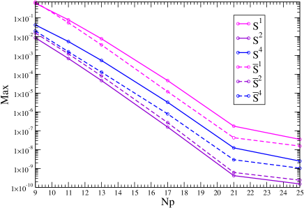
We can see that the maximal value of each component decreases exponentially with the resolution, such a convergence is typical of spectral methods and show that all those values are equal to zero. This successful test validates our 3+1 decomposition of the Simon-Mars tensor, now we consider other stationary, axisymmetric and asymptotically flat spacetimes.

V.2.2 Rotating boson stars

Boson stars are localized configurations of a complex self-gravitating field $\Phi$. Their study is motivated by the fact that they can play the role of black hole mimickers Guzman . For instance, this model presents a viable alternative to the Kerr black hole for the description of the Galactic Center. Mathematically, this is a solution to the coupled system Einstein-Klein-Gordon equations

$$R_{\alpha\beta}-\frac{1}{2}Rg_{\alpha\beta} = 8\pi T_{\alpha\beta},$$ (111)

$$\nabla_{\alpha}\nabla^{\alpha}\Phi = \frac{\textrm{d}V}{\textrm{d}\left|\Phi\right|^{2}}\Phi,$$ (112)

where

$$T_{\alpha\beta}=\nabla_{\left(\alpha\right.}\bar{\Phi}\nabla_{\left.\beta\right)}\Phi-\frac{1}{2}g_{\alpha\beta}\left[\nabla^{\mu}\bar{\Phi}\nabla_{\mu}\Phi+V\left(\left|\Phi\right|^{2}\right)\right].$$ (113)

The potential can take different forms depending on the model we choose for the boson star, here we consider only “mini” boson star formed with a free field potential :

$$V\left(\left|\Phi\right|^{2}\right)=\frac{m^{2}}{\hbar^{2}}\left|\Phi\right|^{2},$$ (114)

where $m$ is the boson mass.

To solve the coupled equations (111) and (112), the following ansatz is used :

$$\Phi=\phi\left(r,\theta\right)\exp\left[i\left(\omega t-k\varphi\right)\right].$$ (115)

A specific boson star is characterized then by the values of $\omega$, which is a real parameter, and $k$, which is an integer (non-rotating boson stars have $k=0$). Given this, the 3+1 decomposition of the matter part (33)-(35) of a boson star is

$$\rho = \left[\frac{\left(\omega+k\beta^{\varphi}\right)^{2}}{N^{2}}+k^{2}h^{\varphi\varphi}\right]\frac{\phi^{2}}{2}$$ (116)

$$+\frac{h^{ij}}{2}\partial_{i}\phi\partial_{j}\phi+\frac{V}{2},$$

$$p_{\varphi} = \frac{k}{N}\left(\omega+k\beta^{\varphi}\right)\phi^{2},$$ (117)

$$S_{ij} = \partial_{\left(i\right.}\bar{\phi}\mathcal{\partial}_{\left.j\right)}\phi$$ (118)

$$+\frac{\gamma_{ij}}{2}\left[\frac{\left(\omega+k\beta^{\varphi}\right)^{2}\phi^{2}}{N^{2}}-\partial_{l}\bar{\phi}\mathcal{\partial}^{l}\phi-V\right].$$

We write then the Einstein-Klein-Gordon equations (111) and (112) in 3+1 form using quasi-isotropic coordinates (see Rotstar ), and those equations are numerically solved by Kadath (see GSG14 for details). More on boson stars can be found in Rev ; Rev 2 (and in references of GSG14 ).

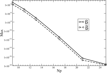
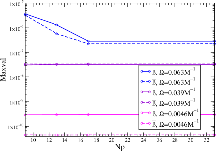
Let us plot in Fig. 2 the same quantities we did for Kerr in Fig. 1, that is to say the maximal values of $\ss$ and $\bar{\ss}$ for several rotating boson stars as functions of the resolution.

Figure 2: Maximal values $\ss$ and $\bar{\ss}$ as functions of the number of spectral coefficients in both the radial and angular dimension for boson stars with the free field potential (114) for $\omega=0.8\,m/\hbar=1.05\,M^{-1}$ and $k=1,2$.

Contrary to the case of Kerr spacetime, the maximal values of $\ss$ and $\bar{\ss}$ do not depend on the resolution up to a certain precision. The conclusion is that it is not zero. The rest of this paper, exploring the same quantities for other spacetimes will permit us to give a meaning to the maximal value found for $\ss$ and $\bar{\ss}$. Furthermore, thanks to Fig. 2, we can choose a fine resolution for the following plots, which will be $17$ points in $r$ and $\theta$.

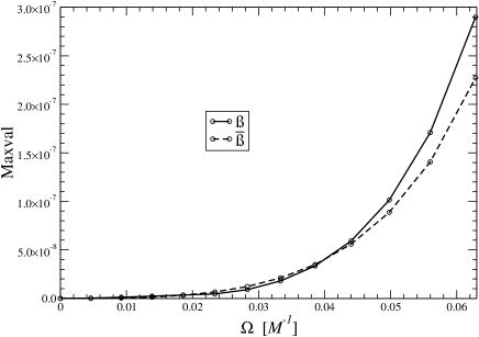
We can also explore the global behavior of the maximal values of $\ss$ and $\bar{\ss}$ for different boson stars for a fixed resolution. For instance, we plot in Fig. 3 those values as functions of $\omega$ for various boson stars.

Figure 3: Maximal values $\ss$ and $\bar{\ss}$ as functions of $\omega$ for boson stars with $k=1,2,3$. As we recover Minkowski spacetime when $\omega\rightarrow 1$ (in units of $\left[m/\hbar\right]$, see GSG14 ), we expect that these values tend to zero which is the case.

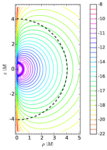
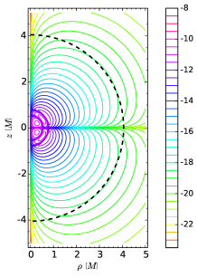
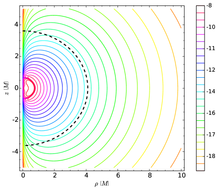
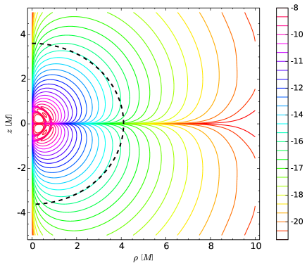
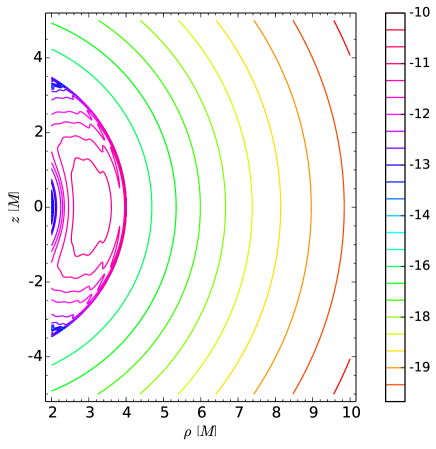
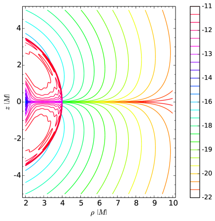
To see how the Simon-Mars scalars behave locally, we present in Fig. 4 and 5 contour plots of $\log\left(\ss\right)$ and $\log\left(\bar{\ss}\right)$ in the equatorial plane as functions of the quasi-isotropic version of the Weyl-Papapetrou coordinates : $r$ and $z$. As the scalar field $\phi$ decreases exponentially fast after reaching its maximum, it makes sense to plot $\log\left(\ss\right)$ and $\log\left(\bar{\ss}\right)$.

Figure 4: Contour plot of $\log\left(\ss\right)$ and $\log\left(\bar{\ss}\right)$ as functions of $r$ and $z$ for a specific boson star characterized by $\omega=1.05\,M^{-1}$ and $k=1$. The lengths are given in units of the ADM mass of each boson star, to make the two plots comparable. The black point marks the position of the maximal value of the boson star field, and the dotted line indicate the positions where the field take the value $\phi_{\textrm{max}}/10$.

Figure 5: Same figure as Fig. 4 for the boson star characterized by $\omega=0.67\,M^{-1}$ and $k=1$. The grey dashed line marks the location of the ergoregion.

V.2.3 Rotating neutron stars

Another example of stationary, axisymmetric and asymptotically flat spacetime with a matter content, for which the metric can also be expressed in quasi-isotropic coordinates is the model of rotating neutron stars. Contrary to boson stars, the matter content is a perfect fluid. The stress tensor has the following form

$$T_{\alpha\beta}=\left(\varepsilon+p\right)u_{\alpha}u_{\beta}+pg_{\alpha\beta},$$ (119)

where $u^{\alpha}$ is the unit timelike vector field representing the fluid 4-velocity, $\varepsilon$ and $p$ are the two scalar fields representing respectively the energy density and the pressure of the fluid. The 3+1 decomposition of the 4-velocity of the fluid with respect to the Eulerian observer 4-velocity $\vec{n}$ is

$$u^{\alpha}=\Gamma\left(n^{\alpha}+U^{\alpha}\right),$$ (120)

where $\Gamma=-n^{\mu}u_{\mu}$ is the Lorentz factor of the fluid with respect to the Eulerian observer and the 3-velocity of the fluid with respect also to this Eulerian observer is Rotstar

$$U^{\alpha}=\frac{B}{N}\left(\Omega-N^{\varphi}\right)r\sin\theta,$$ (121)

where $\Omega$ is the orbital angular velocity with respect to a distant inertial observer. The normalization condition $u^{\mu}u_{\mu}=-1$ gives

$$\Gamma=\frac{1}{\sqrt{1-U^{2}}}.$$ (122)

So the 3+1 matter content (33)-(35) can be written

$$\rho = \Gamma^{2}\left(\varepsilon+p\right)-p$$ (123)

$$p_{\alpha} = \Gamma^{2}\left(\varepsilon+p\right)U_{\alpha}$$ (124)

$$S_{\alpha\beta} = \Gamma^{2}\left(\varepsilon+p\right)U_{\alpha}U_{\beta}+p\,h_{\alpha\beta}.$$ (125)

In order to close the system, we consider a polytropic equation of state with $\gamma=2$. To read more about neutron stars and how these objects are computed numerically see Gourg01 and references therein.

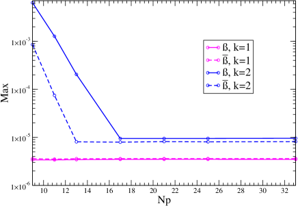
We plot in Fig. 6 the maximal values of $\ss$ and $\bar{\ss}$ for a static and several rotating neutron stars as functions of the resolution.

Figure 6: Maximal values of $\ss$ and $\bar{\ss}$ as functions of the number of spectral coefficients in both the radial and angular dimension for neutron stars with for $\Omega=0.0046,0.039,0.063\>M^{-1}$ .

As in the boson star case, the maximal values of $\ss$ and $\bar{\ss}$ do not depend on the resolution up to a certain precision. We choose the resolution of $17$ points in $r$ and $\theta$ for the following plots.

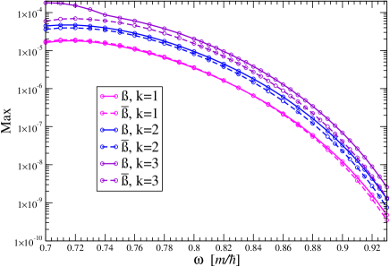
We can explore the global behavior of the maximal values of $\ss$ and $\bar{\ss}$ for different neutron stars for a fixed resolution. For instance, we plot in Fig. 7 those maximal values as functions of $\Omega$ for different rotating neutron stars.

Figure 7: Maximal values of $\ss$ and $\bar{\ss}$ as functions of $\Omega$ for rotating neutron stars. When $\Omega\rightarrow 0$, the neutron star is less rapidly rotating (static for $\Omega=0$) and the spacetime becomes closer to the Schwarzschild solution.

Figures 8 and 9 show contours of $\log\left(\ss\right)$ and $\log\left(\bar{\ss}\right)$ for two different neutron stars.

Figure 8: Contour plot of $\log\left(\ss\right)$ as a function of $r$ and $z$ for a rotating neutron star with $\Omega=0.0046\>M^{-1}$. The black dashed line indicates the position of the surface of the neutron star.

Figure 9: Contour plots of $\log\left(\ss\right)$ and $\log\left(\bar{\ss}\right)$ as functions of $r$ and $z$ for a rotating neutron star with $\Omega=0.039\>M^{-1}$.

V.3 Exact analytic solutions of the Einstein equations

It is interesting also to compare the values of the Simon-Mars scalars we obtain in the two preceding examples to other spacetimes. We chose to do it with two specific spacetimes for which the difference to Kerr has been already quantified in GLS13 , one is the Curzon-Chazy spacetime first studied by Curzon in Curzon and Chazy in Chazy , the other is the $\delta=2$ Tomimatsu-Sato spacetime defined in Tom72 .

Calculating the Simon-Mars scalars for these spacetimes permits us to put a link between our characterization of the “non-Kerness” and the characterization with invariants given in GLS13 . This classification is more fine than ours because is uses more than the Simon-Mars tensor. But it is based on vacuum spacetime, or very small deviation from vacuum spacetimes while ours can be applied to all spacetimes. Thus, our scalar calculation can advantageously complete their classification providing invariants that can be calculated even for non vacuum spacetimes such as the two examples treated in the preceding section.

Even if there are more examples in GLS13 , in most of them (which are not vacuum solutions of the Einstein equations, so Mars theorem does not hold), the Simon-Mars is zero, so we focus in the solutions that are in vacuum and not locally isomorphic to Kerr (their Simon-Mars tensor cannot be zero). For this part, we used the SageManifolds free package GourgBM14 ; SageManifolds , which is an extension towards differential geometry and tensor calculus of the open-source mathematics software Sage Sage .

V.3.1 Exact vacuum axisymmetric solutions

As we saw in section IV.1, the metric of a generic stationary, axisymmetric and circular spacetime can be written in quasi-isotropic coordinates (89) : $\left(t,r,\theta,\varphi\right)$. The related cylindrical coordinates $\left(t,\rho,z,\varphi\right)$ with $\rho=r\sin\theta$ and $z=r\cos\theta$ are the Weyl-Lewis-Papapetrou coordinates :

$$\textrm{d}s^{2} = -e^{2U}\left(\textrm{d}t+\beta^{\varphi}\rho\textrm{d}\varphi\right)^{2}$$ (126)

$$+e^{-2U}\left[e^{2\gamma}\left(\textrm{d}\rho^{2}+\textrm{d}z^{2}\right)+\rho^{2}\textrm{d}\varphi^{2}\right],$$

where $U$ and $\gamma$ are functions of $\rho$ and $z$. In these coordinates, $U$ and $\gamma$ play the same role of $A,\,B$ and $N$ in the quasi-isotropic coordinates : indeed, in vacuum, $B=1/N$ (see eq. (3.16) of Rotstar ). Writing the vacuum Einstein field equations satisfied by this metric, we obtain a single differential equation, called the Ernst equation, for a complex potential, called the Ernst potential Ernst . This equation is integrable so it can be solved by various solutions generating techniques : in the static case ($\beta^{\varphi}=0$), a family of asymptotically flat solutions can be found expressing $U$ as a sum of Legendre polynomials. This family is called the Weyl class GP and Curzon-Chazy spacetime is the simplest member of this class.

For stationary (but not static) axisymmetric solutions, it is convenient to write the Ernst equation in prolate spherical coordinates $\left(x,y\right)$ related to the Weyl-Lewis-Papapetrou coordinates $\left(\rho,z\right)$ by

$$x = \frac{1}{2}\left(\sqrt{\rho^{2}+\left(z+1\right)^{2}}+\sqrt{\rho^{2}+\left(z-1\right)^{2}}\right)$$ (127)

$$y = \frac{1}{2}\left(\sqrt{\rho^{2}+\left(z+1\right)^{2}}-\sqrt{\rho^{2}+\left(z-1\right)^{2}}\right),$$ (128)

where $x\geq 1$ and $y\in\left[-1,1\right]$. Tomimatsu and Sato Tom72 ; Sato73 have labeled the solutions by a deformation parameter called $\delta$. The solution corresponding to $\delta=1$, the simplest one, is the Kerr one. The solution which we consider in this paper is the $\delta=2$ Tomimatsu-Sato solution.

V.3.2 Kerr spacetime

As a test of the SageManifolds code, we evaluated the Simon-Mars tensor (11) for the Kerr metric in Boyer-Lindquist coordinates and we evaluated also each of the eight 3+1 components of the Simon-Mars tensor : (77)-(80) and (82)-(85). We found identically zero. This computations confirms that the same results are found with the original definition and with the 3+1 decomposition. Furthermore, it validates the use of SageManifolds worksheets. The latter are freely downloadable from SM_examples .

V.3.3 Curzon-Chazy spacetime

The Curzon-Chazy spacetime is a static, axisymmetric and asymptotically flat solution of the Einstein equations Curzon ; Chazy . Its line element is given by the Weyl-Lewis-Papapetrou one with $\beta^{\varphi}=0$ and

$$U=-\frac{M}{r},\;\gamma=-\frac{M^{2}\sin^{2}\theta}{2r^{2}}.$$ (129)

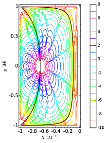
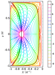
It has a spherically symmetric Newtonian potential, corresponding to the potential of a point particle of mass $M$ located at $r=0$, where lies a singularity of complex nature, but this spacetime is not spherically symmetric. Because the shift is zero for this spacetime, $\bar{\ss}$ is identically null, so we can only show the contour plot of $\log\left(\ss\right)$ in Fig. 10.

Figure 10: Contour plots of $\log\left(\ss\right)$ for Curzon-Chazy spacetime as a function of $\rho$ and $z$ for $M=1$ and for $M=12$.

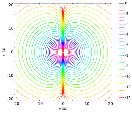
The computation of the Simon-Mars scalars has been performed with SageManifolds (the corresponding worksheet is available at SM_examples ). As this solution is analytic, we identified those scalars both with their 3+1 definitions (87) and (88), but also as the real and imaginary part of the “square” of the 4-dimensional Simon-Mars scalar (86).

First we see that the Simon-Mars scalars diverge at the singularity. For vacuum spacetimes, the Weyl tensor is equal to the Riemann tensor, so the Simon-Mars are close to the Kretchmann with diverge at each real singularity (not coordinate singularities) of the metric, so we can expect this behavior. Furthermore, comparing with Fig. 1 of GLS13 , we can confirm that the adapted quantity is $\log\left(\ss\right)$ and not $\ss$ by comparing the shape of the contours, we can also see that a spherically symmetric spacetime differs little to the Kerr spacetime when $\log\left(\ss\right)<-8$. In this sense, at the singularity the Curzon-Chazy spacetime is infinitely far from the Kerr spacetime, which is not false.

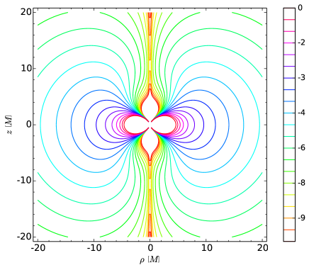
V.3.4 $\delta=2$ Tomimatsu-Sato spacetime

This spacetime, which is defined in Tom72 ; Sato73 , is a stationary, axisymmetric vacuum solution of the Einstein equations which is also asymptotically flat (see Glass73 ). This metric is one of the rare stationary and axisymmetric exact solutions of Einstein equations. The non zero elements of the metric are

$$g_{tt} = -\frac{A\left(x,y\right)}{B\left(x,y\right)},$$ (130)

$$g_{t\varphi} = -\frac{2Mq\left(x,y\right)C\left(x,y\right)\left(1-y^{2}\right)}{B\left(x,y\right)},$$ (131)

$$g_{xx} = \frac{M^{2}B\left(x,y\right)}{p^{2}\delta^{2}\left(x^{2}-1\right)\left(x^{2}-y^{2}\right)^{3}},$$ (132)

$$g_{yy} = \frac{M^{2}B\left(x,y\right)}{p^{2}\delta^{2}\left(y^{2}-1\right)\left(y^{2}-x^{2}\right)^{3}},$$ (133)

$$g_{\varphi\varphi} = \frac{M^{2}\left(y^{2}-1\right)p^{2}B^{2}\left(x,y\right)\left(x^{2}-1\right)}{A\left(x,y\right)B\left(x,y\right)\delta^{2}}$$ (134)

$$+4\frac{q^{2}\delta^{2}C^{2}\left(x,y\right)\left(y^{2}-1\right)}{A\left(x,y\right)B\left(x,y\right)\delta^{2}},$$

with

$$A\left(x,y\right) = \left[p^{2}\left(x^{2}-1\right)^{2}+q^{2}\left(1-y^{2}\right)^{2}\right]^{2}$$ (135)

$$-4p^{2}q^{2}\left(x^{2}-1\right)\left(1-y^{2}\right)\left(x^{2}-y^{2}\right)^{2},$$

$$B\left(x,y\right) = \left(p^{2}x^{4}+q^{2}y^{4}-1+2px^{3}-2px\right)^{2}$$ (136)

$$+4q^{2}y^{2}\left(px^{3}-pxy^{2}+1-y^{2}\right)^{2},$$

$$C\left(x,y\right) = p^{2}\left(x^{2}-1\right)\left[\left(x^{2}-1\right)\left(1-y^{2}\right)-4x^{2}\left(x^{2}-y^{2}\right)\right]$$ (137)

$$-p^{3}x\left(x^{2}-1\right)\left[2\left(x^{4}-1\right)+\left(x^{2}+3\right)\left(1-y^{2}\right)\right]$$

$$+q^{2}\left(1+px\right)\left(1-y^{2}\right)^{3},$$

where $p$ and $q$ are real constant satisfying the constraint $p^{2}+q^{2}=1$, and $M$ is the ADM mass, here we choose $p=1/5$, and $M=1$.

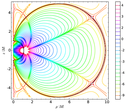
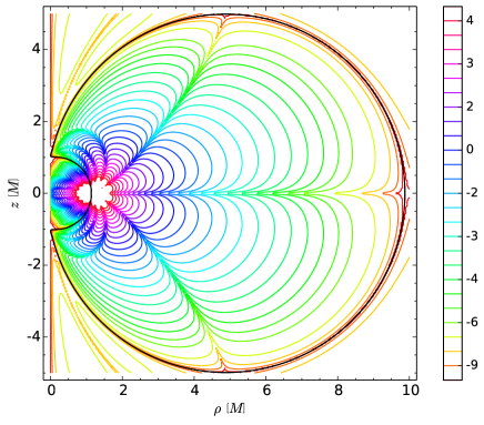
This spacetime contains two degenerated Killing horizons at $x=1$, $y=\pm 1$, and a naked ring singularity (more on the $\delta=2$ Tomimatsu-Sato spacetime in Manko ). The computation of the two Simon-Mars scalars starting from the metric (130)-(137) is rather formidable. We performed it by means of the SageManifolds code mentioned above. The corresponding worksheet is available at SM_examples .

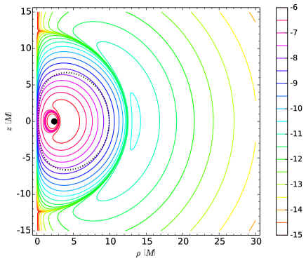
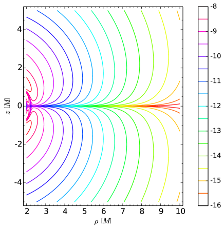
In Fig. 11, we show the contour plots of $\log\left(\ss\right)$ and $\log\left(\bar{\ss}\right)$ as functions of $X=-1/x$ and $y$ (given by (127) and (128)) to compare our result to the Fig. 2 of GLS13 . We see that the order of magnitude of the two scalars is the same. But is is harder to make a comparison with Fig. 2 of GLS13 in this case because the scalars grow exponentially around the singularity, which is not the case in GLS13 . Nevertheless we can compare the value of the scalars along the horizontal axis ($y=0$), and we see that in this case an axisymmetric spacetime seems to differ little to the Kerr spacetime when $\log\left(\ss\right)<-6$. Outside the ergosphere the values of $\log\left(\ss\right)$ and $\log\left(\bar{\ss}\right)$ diminish frankly.

Figure 11: Contour plots of $\log\left(\ss\right)$ and $\log\left(\bar{\ss}\right)$ for $\delta=2$ Tomimatsu-Sato spacetime for $p=1/5$ and $M=1$ and as functions of $X=-1/x$ and $y$. The black line marks the ergosurface. The scalars diverge at the naked ring singularity.

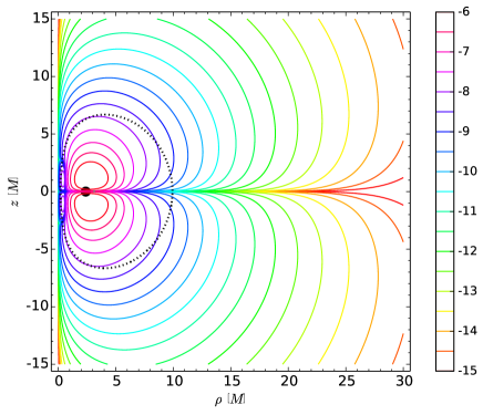
We do the same plot in the Weyl-Lewis-Papapetrou coordinates which are more usual coordinates (see Manko ), in Fig. 12.

Figure 12: Same plot as in Fig. 11 in Weyl-Lewis-Papapetrou coordinates $\rho$ and $z$.

V.4 Approximate solution : the Modified Kerr metric

The modified Kerr metric proposed by Johannsen and Psaltis JoPs is a family of approximate solutions of the Einstein field equations, which are non linear parametric deviations from the Kerr metric. The line element is given in Boyer-Lindquist coordinates by

$$\textrm{d}s^{2} = -\left[1+h\left(r,\theta\right)\right]\left(1-\frac{2Mr}{\Sigma}\right)\textrm{d}t^{2}-\frac{4aMr\sin^{2}\theta}{\Sigma}$$ (138)

$$\times\left[1+h\left(r,\theta\right)\right]\textrm{d}t\textrm{d}\varphi+\frac{\Sigma\left[1+h\left(r,\theta\right)\right]}{\Delta+a^{2}\sin^{2}\theta h\left(r,\theta\right)}\textrm{d}r^{2}$$

$$+\Sigma\textrm{d}\theta^{2}+\left[\sin^{2}\theta\left(r^{2}+a^{2}+\frac{2a^{2}Mr\sin^{2}\theta}{\Sigma}\right)\right.$$

$$+\left.h\left(r,\theta\right)\frac{a^{2}\left(\Sigma+2Mr\right)\sin^{4}\theta}{\Sigma}\right]\textrm{d}\varphi^{2},$$

where $a$ is the specific angular momentum of the black hole, $M$ its ADM mass and

$$\Sigma = r^{2}+a^{2}\cos^{2}\theta$$ (139)

$$\Delta = r^{2}-2Mr+a^{2}.$$ (140)

The simplest choice for $h\left(r,\theta\right)$ in accordance with the observational constraints on weak-field deviations from general relativity is given by

$$h\left(r,\theta\right)=\epsilon_{3}\frac{M^{3}r}{\Sigma^{2}}.$$ (141)

This spacetime is a black hole only for certain values of $\epsilon_{3}$ and $a$ (see Fig. 3 of Jo13 ) : if $0\leq a\leq 0.8\>M$ and $-5\leq\epsilon_{3}\leq 0$, it is always the case. In this paper, we focus on this particular zone, so we use the positive parameter $\epsilon=-\epsilon_{3}$.

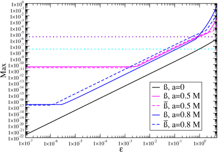
In Fig. 13, we plot the maximal values of $\ss$ and $\bar{\ss}$ as functions of $\varepsilon$ for different values of the spin. We see that the bigger $a$ is, the bigger is the lowest maximal value of the scalars, meaning that the more this modified Kerr black hole is rapidly rotating, the more it differs for the Kerr original solution. The idea was to quantify the deviation to the Kerr spacetime of the preceding examples by seeing how fast the two Simon-Mars scalars evaluated in the modified Kerr metric deviate from zero.

For spacetimes containing singularities as the Curzon-Chazy solution and the $\delta=2$ Tomimatsu-Sato spacetime, the characterization of their “non-Kerness” can be only local because the two scalars diverge at the singularities. But for smooth spacetimes such as boson stars or neutron stars, we can report the maximal values of the scalars on the Fig. 13, as we did for one specific example of each. We can say that the spacetime generated by the neutron star chosen is more close to the Kerr spacetime than the spacetime generated by the boson star. This corresponds to our intuition because the boson star shape is a torus, and it seems a more exotic object than the neutron star.

Figure 13: Maximal values $\ss$ and $\bar{\ss}$ as functions of $\epsilon$ for modified Kerr metrics with $a=0,0.5,0.8\>M$. As the deviation from the Kerr metric is non linear, we use a log-log scale. The violet dotted line corresponds to the maximal value of $\ss$ ($\ss=3.48826.10^{-6}$) for the boson star with $\omega=1.05\,M^{-1}$ and $k=1$, and the cyan dotted line corresponds to the maximal value of $\ss$ ($\ss=3.34572.10^{-8}$) for the neutron star with $\Omega=0.039\>M^{-1}$.

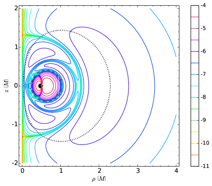
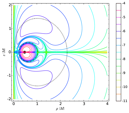
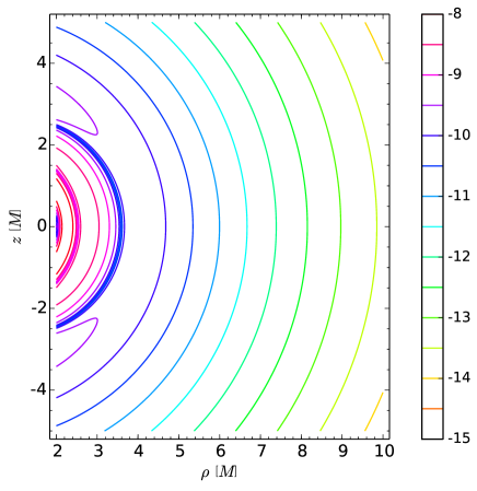
To see local configurations of the scalar fields for examples of modified Kerr spacetimes, we present contour plots of $\log\left(\ss\right)$ and $\log\left(\bar{\ss}\right)$ for chosen values of $\epsilon$ and $a$ in Fig. 14 and 15. As the topology of the event horizon is not simple in this geometry (see Jo13 ) and as it is located in the zone where $r<2\,M$, we choose to plot only the outer domain for $r\geq 2\,M$. The scalar values are very small compared to the other solutions, which is reassuring because this example is supposed to be very close to the Kerr spacetime.

Figure 14: Contour plot of $\log\left(\ss\right)$ and $\log\left(\bar{\ss}\right)$ as functions of $r\geq 2\,M$ and $z$ for a modified Kerr metric with $a=0.5\>M$ and $\epsilon=10^{-4}$.

Figure 15: Same plots as Fig. 14 a modified Kerr metric with $a=0.8\>M$ and $\varepsilon=0.1$.

VI Conclusion

We performed the 3+1 decomposition of the Simon-Mars tensor, and defined two scalar fields from it. It permitted us to quantify the deviation of different spacetimes to the Kerr one by evaluating these scalars. This classification works only for stationary spacetimes, but can be applied to non vacuum spacetimes, and especially in numerical spacetimes with a matter content, what could not be done before, as far as we know. Nevertheless, in some of these non-vacuum spacetimes, the scalar fields can be identically zero even if the spacetime is not locally isometric to the Kerr spacetime, because the Mars theorem does not hold in non-vacuum spacetimes. Thus one has to be careful using this characterization of Kerr spacetime, which provides an efficient way to compare different spacetimes to one another.

References

- (1) R. P. Kerr, Phys. Rev. Lett. 11, 237 (2005).
- (2) R. Genzel, F. Eisenhauer, S. Gillessen, Rev. Mod. Phys., 82, 3121 (2010).
- (3) P. Grandclément, C. Somé, E. Gourgoulhon, Phys. Rev. D 90, 024068 (2014).
- (4) S. L. Liebling, C. Palenzuela, Living Rev. Relativity, 15, 6, (2012).
- (5) M. Mars, Class. Quantum Grav. 16, 2507 (1999).
- (6) E. Cotton, Annales de la fac. des sciences de Toulouse série, tome 1, 4 (1899).
- (7) W. Simon, Gen. Relativ. Gravit., 16, 5 (1984).
- (8) D. Bini, R. T. Jantzen, G. Miniutti, Class. Quantum Grav. 18, 4969 (2001).
- (9) A. D. Ionescu, S. Klainerman, Invent. Math. 175 (1), 35–102 (2009).
- (10) A. García-Parrado Gómez-Lobo, J. A. Valiente Kroon, Class. Quantum Grav. 25, 205018 (2008).
- (11) A. García-Parrado Gómez-Lobo, J. M. M. Senovilla, Gen. Relativ. Gravit., 45, 6 (2013).
- (12) T. Bäckdahl, J. A. Valiente Kroon, Proc. R. Soc. A., 467, 1701 (2011).
- (13) T. Johannsen, D. Psaltis, Phys. Rev. D 83, 124015 (2011).
- (14) M. Mars, Class. Quantum Grav. 17, 3353 (2000).
- (15) E. Gourgoulhon, 3+1 Formalism in General Relativity. Bases of Numerical Relativity, (Springer, Berlin, 2012).
- (16) M. Alcubierre, Introduction to 3+1 Numerical Relativity, (Oxford Univ. Press, Oxford, 2008).
- (17) A. Matte, Can. J. Math. 5, 1 (1953).
- (18) J. A. Valiente Kroon, Conformal methods in General Relativity, (Cambridge University Press, in preparation).
- (19) E. Gourgoulhon, An introduction to the theory of rotating relativistic stars, lectures given at CompStar 2010 School (Caen, 8-16 Feb 2010), available as arXiv1003.5015.
- (20) R. Wald, General Relativity, (University of Chicago Press, 1984).
- (21) E. Gourgoulhon, Black hole spacetimes in Quasi-isotropic coordinates, unpublished.
- (22) P. Grandclément, J. Comp. Phys. 229, 3334 (2010).
- (23) http://luth.obspm.fr/~luthier/grandclement/kadath.html
- (24) E. Gourgoulhon, M. Bejger and M. Mancini, in Proceedings of ERE2014: Almost 100 years after Einstein’s revolution, J. Phys.: Conf. Ser., in press; preprint arXiv1412.4765
- (25) http://sagemanifolds.obspm.fr/
- (26) E. Gourgoulhon et al., Phys. Rev. D 63, 064029 (2001).
- (27) F. S. Guzman and J. M. Rueda-Becerril, Phys. Rev. D 80, 084023 (2009).
- (28) F. E. Schunck and E. W. Mielke, Class. Quantum Grav. 20, 301 (2003).
- (29) H. E. J. Curzon, Proc. London Math. Soc, 23, 477–480 (1924).
- (30) J. Chazy, Bull. Soc. Math. France, 52, 17 (1924).
- (31) A. Tomimatsu and H. Sato, Phys. Rev. Lett. 29, 1344 (1972).
- (32) http://www.sagemath.org/
- (33) A. Tomimatsu and H. Sato, Prog. Theor. Phys., 50, 95 (1973).
- (34) F. J. Ernst, Phys. Rev. 167, 5 (1967).
- (35) J. B. Griffiths, J. Podolský, Exact Space-Times in Einstein’s General Relativity, (Cambridge Monographs on Mathematical Physics, 2012).
- (36) http://sagemanifolds.obspm.fr/examples.html
- (37) E. N. Glass, Phys. Rev. D 7, 10 (1973).
- (38) V. S. Manko, Prog. Theor. Phys., 127, 6 (2012).
- (39) T. Johannsen, Phys. Rev. D 87, 124017 (2013).