A la Carte — Learning Fast Kernels

Abstract

Kernel methods have great promise for learning rich statistical representations of large modern datasets. However, compared to neural networks, kernel methods have been perceived as lacking in scalability and flexibility. We introduce a family of fast, flexible, lightly parametrized and general purpose kernel learning methods, derived from Fastfood basis function expansions. We provide mechanisms to learn the properties of groups of spectral frequencies in these expansions, which require only $\mathcal{O}(m\log d)$ time and $\mathcal{O}(m)$ memory, for $m$ basis functions and $d$ input dimensions. We show that the proposed methods can learn a wide class of kernels, outperforming the alternatives in accuracy, speed, and memory consumption.

1 Introduction

The generalisation properties of a kernel method are entirely controlled by a kernel function, which represents an inner product of arbitrarily many basis functions. Kernel methods typically face a tradeoff between speed and flexibility. Methods which learn a kernel lead to slow and expensive to compute function classes, whereas many fast function classes are not adaptive. This problem is compounded by the fact that expressive kernel learning methods are most needed on large modern datasets, which provide unprecedented opportunities to automatically learn rich statistical representations.

For example, the recent spectral kernels proposed by Wilson and Adams (2013) are flexible, but require an arbitrarily large number of basis functions, combined with many free hyperparameters, which can lead to major computational restrictions. Conversely, the recent Random Kitchen Sinks of Rahimi and Recht (2009) and Fastfood (Le et al., 2013) methods offer efficient finite basis function expansions, but only for known kernels, a priori hand chosen by the user. These methods do not address the fundamental issue that it is exceptionally difficult to know a-priori which kernel might perform well; indeed, an appropriate kernel might not even be available in closed form.

We introduce a family of kernel learning methods which are expressive, scalable, and general purpose. In particular, we introduce flexible kernels, including a novel piecewise radial kernel, and derive Fastfood basis function expansions for these kernels. We observe that the frequencies in these expansions can in fact be adjusted, and provide a mechanism for automatically learning these frequencies via marginal likelihood optimisation. Individually adjusting these frequencies provides the flexibility to learn any translation invariant kernel. However, such a procedure has as many free parameters as basis functions, which can lead to over-fitting, troublesome local optima, and computational limitations. We therefore further introduce algorithms which can control the scales, spread, and locations of groups of frequencies. These methods are computationally efficient, and allow for great flexibility, with a minimal number of free parameters requiring training. By controlling groups of spectral frequencies, we can use arbitrarily many basis functions with no risk of over-fitting. Furthermore, these methods do not require the input data have any special structure (e.g., regular sampling intervals).

Overall, we introduce four new kernel learning methods with distinct properties, and evaluate each of these methods on a wide range of real datasets. We show major advantages in accuracy, speed, and memory consumption. We begin by describing related work in more detail in section 2. We then provide additional background on kernel methods, including basic properties and Fastfood approximations, in section 3. In section 4 we introduce a number of new tools for kernel learning. Section 5 contains an evaluation of the proposed techniques on many datasets. We conclude with a discussion in section 6.

2 Related Work

Rahimi and Recht (2008) introduced Random Kitchen Sinks finite Fourier basis function approximations to fixed stationary kernels, using a Monte Carlo sum obtained by sampling from spectral densities. For greater flexibility, one can consider a weighted sum of random kitchen sink expansions of Rahimi and Recht (2009). In this case, the expansions are fixed, corresponding to a-priori chosen kernels, but the weighting can be learned from the data.

Recently, Lu et al. (2014) have shown how weighted sums of random kitchen sinks can be incorporated into scalable logistic regression models. First, they separately learn the parameters of multiple logistic regression models, each of which uses a separate random kitchen sinks expansion, enabling parallelization. They then jointly learn the weightings of each expansion. Learning proceeds through stochastic gradient descent. Lu et al. (2014) achieve promising performance on acoustic modelling problems, in some instances outperforming deep neural networks.

Alternatively, Lázaro-Gredilla et al. (2010) considered optimizing the locations of all spectral frequencies in Random Kitchen Sinks expansions, as part of a sparse spectrum Gaussian process formalism (SSGPR).

For further gains in scalability, Le et al. (2013) approximate the sampling step in Random Kitchen Sinks by a combination of matrices which enable fast computation. The resulting Fastfood expansions perform similarly to Random Kitchen Sinks expansions (Le et al., 2013), but can be computed more efficiently. In particular, the Fastfood expansion requires $\mathcal{O}(m\log d)$ computations and $\mathcal{O}(m)$ memory, for $m$ basis functions and $d$ input dimensions.

To allow for highly flexible kernel learning, Wilson and Adams (2013) proposed spectral mixture kernels, derived by modelling a spectral density by a scale-location mixture of Gaussians. These kernels can be computationally expensive, as they require arbitrarily many basis functions combined with many free hyperparameters. Recently, Wilson et al. (2014) modified spectral mixture kernels for Kronecker structure, and generalised scalable Kronecker (Tensor product) based learning and inference procedures to incomplete grids. Combining these kernels and inference procedures in a method called GPatt, Wilson et al. (2014) show how to learn rich statistical representations of large datasets with kernels, naturally enabling extrapolation on problems involving images, video, and spatiotemporal statistics. Indeed the flexibility of spectral mixture kernels makes them ideally suited to large datasets. However, GPatt requires that the input domain of the data has at least partial grid structure in order to see efficiency gains.

In our paper, we consider weighted mixtures of Fastfood expansions, where we propose to learn both the weighting of the expansions and the properties of the expansions themselves. We propose several approaches under this framework. We consider learning all of the spectral properties of a Fastfood expansion. We also consider learning the properties of groups of spectral frequencies, for lighter parametrisations and useful inductive biases, while retaining flexibility. For this purpose, we show how to incorporate Gaussian spectral mixtures into our framework, and also introduce novel piecewise linear radial kernels. Overall, we show how to perform simultaneously flexible and scalable kernel learning, with interpretable, lightly parametrised and general purpose models, requiring no special structure in the data. We focus on regression for clarity, but our models extend to classification and non-Gaussian likelihoods without additional methodological innovation.

3 Kernel Methods

3.1 Basic Properties

Denote by $\mathcal{X}$ the domain of covariates and by $\mathcal{Y}$ the domain of labels. Moreover, denote $X:=\left\{x_{1},\ldots,x_{n}\right\}$ and $Y:=\left\{y_{1},\ldots,y_{n}\right\}$ data drawn from a joint distribution $p$ over $\mathcal{X}\times\mathcal{Y}$. Finally, let $k:\mathcal{X}\times\mathcal{X}\to\mathbb{R}$ be a Hilbert Schmidt kernel (Mercer, 1909). Loosely speaking we require that $k$ be symmetric, satisfying that every matrix $K_{ij}:=k(x_{i},x_{j})$ be positive semidefinite, $K\succeq 0$.

The key idea in kernel methods is that they allow one to represent inner products in a high-dimensional feature space implicitly using

$$k(x,x^{\prime})=\left\langle\phi(x),\phi(x^{\prime})\right\rangle.$$ (1)

While the existence of such a mapping $\phi$ is guaranteed by the theorem of Mercer (1909), manipulation of $\phi$ is not generally desirable since it might be infinite dimensional. Instead, one uses the representer theorem (Kimeldorf and Wahba, 1970; Schölkopf et al., 2001) to show that when solving regularized risk minimization problems, the optimal solution $f(x)=\left\langle w,\phi(x)\right\rangle$ can be found as linear combination of kernel functions:

$$\left\langle w,\phi(x)\right\rangle=\left\langle\sum_{i=1}^{n}\alpha_{i}\phi(x_{i}),\phi(x)\right\rangle=\sum_{i=1}^{n}\alpha_{i}k(x_{i},x).$$

While this expansion is beneficial for small amounts of data, it creates an unreasonable burden when the number of datapoints $n$ is large. This problem can be overcome by computing approximate expansions.

3.2 Fastfood

The key idea in accelerating $\left\langle w,\phi(x)\right\rangle$ is to find an explicit feature map such that $k(x,x^{\prime})$ can be approximated by $\sum_{j=1}^{m}\psi_{j}(x)\psi_{j}(x^{\prime})$ in a manner that is both fast and memory efficient. Following the spectral approach proposed by Rahimi and Recht (2009) one exploits that for translation invariant kernels $k(x,x^{\prime})=\kappa(x-x^{\prime})$ we have

$$k(x,x^{\prime})=\int\rho(\omega)\exp\left(i\left\langle\omega,x-x^{\prime}\right\rangle\right)d\omega\,.$$ (2)

Here $\rho(\omega)=\rho(-\omega)\geq 0$ to ensure that the imaginary parts of the integral vanish. Without loss of generality we assume that $\rho(\omega)$ is normalized, e.g. $\left\|\rho\right\|_{1}=1$. A similar spectral decomposition holds for inner product kernels $k(x,x^{\prime})=\kappa(\left\langle x,x^{\prime}\right\rangle)$ (Le et al., 2013; Schoenberg, 1942).

Rahimi and Recht (2009) suggested to sample from the spectral distribution $\rho(\omega)$ for a Monte Carlo approximation to the integral in (2). For example, the Fourier transform of the popular Gaussian kernel is also Gaussian, and thus samples from a normal distribution for $\rho(\omega)$ can be used to approximate a Gaussian (RBF) kernel.

This procedure was refined by Le et al. (2013) by approximating the sampling step with a combination of matrices that admit fast computation. They show that one may compute Fastfood approximate kernel expansions via

$$\tilde{k}(x,x^{\prime})\propto\frac{1}{m}\sum_{j=1}^{m}\phi_{j}(x)\phi^{*}_{j}(x^{\prime})\text{ where }\phi_{j}(x)=\exp\left(i[SHG\Pi HBx]_{j}\right).$$ (3)

The random matrices $S,H,G,\Pi,B$ are chosen such as to provide a sufficient degree of randomness while also allowing for efficient computation.

$B$ Binary decorrelation

The entries $B_{ii}$ of this diagonal matrix are drawn uniformly from $\left\{\pm 1\right\}$. This ensures that the data have zero mean in expectation over all matrices $B$.

$H$ Hadamard matrix

It is defined recursively via

$$H_{1}:=\left[\begin{array}[]{r}1\end{array}\right]\text{ and }H_{2d}:=\left[\begin{array}[]{rr}H_{d}&H_{d}\\ H_{d}&-H_{d}\end{array}\right]\text{ hence }H_{2d}\left[\begin{array}[]{l}x\\ x^{\prime}\end{array}\right]=\left[\begin{array}[]{l}H_{d}[x+x^{\prime}]\\ H_{d}[x-x^{\prime}]\end{array}\right].$$

The recursion shows that the dense matrix $H_{d}$ admits fast multiplication in $O(d\log d)$ time, i.e. as efficiently as the FFT allows.

$\Pi$ Permutation matrix

This decorrelates the eigensystems of subsequent Hadamard matrices. Generating such a random permutation (and executing it) can be achieved by reservoir sampling, which amounts to $n$ in-place pairwise swaps. It ensures that the spaces of both permutation matrices are effectively uncorrelated.

$G$ Gaussian matrix

It is a diagonal matrix with Gaussian entries drawn iid via $G_{ii}\sim\mathcal{N}(0,1)$. The result of using it is that each of the rows of $HG\Pi HB$ consist of iid Gaussian random variables. Note, though, that the rows of this matrix are not quite independent.

$S$ Scaling matrix

This diagonal matrix encodes the spectral properties of the associated kernel. Consider $\rho(\omega)$ of (2). There we draw $\omega$ from the spherically symmetric distribution defined by $\rho(\omega)$ and use its length to rescale $S_{ii}$ via

$$S_{ii}=\left\|\omega_{i}\right\|\left\|G\right\|^{-1}_{\mathrm{Frob}}$$

It is straightforward to change kernels, for example, by adjusting $S$. Moreover, all the computational benefits of decomposing terms via (3) remain even after adjusting $S$. Therefore we can customize kernels for the problem at hand rather than applying a generic kernel, without incurring additional computational expenses.

4 À la Carte

In keeping with the culinary metaphor of Fastfood, we now introduce a flexible and efficient approach to kernel learning à la carte. That is, we will adjust the spectrum of a kernel in such a way as to allow for a wide range of translation-invariant kernels. Note that unlike previous approaches, this can be accomplished without any additional cost since these kernels only differ in terms of their choice of scaling.

In Random Kitchen Sinks and Fastfood, the frequencies $\omega$ are sampled from the spectral density $\rho(\omega)$. One could instead learn the frequencies $\omega$ using a kernel learning objective function. Moreover, with enough spectral frequencies, such an approach could learn any stationary (translation invariant) kernel. This is because each spectral frequency corresponds to a point mass on the spectral density $\rho(\omega)$ in (2), and point masses can model any density function.

However, since there are as many spectral frequencies as there are basis functions, individually optimizing over all the frequencies $\omega$ can still be computationally expensive, and susceptible to over-fitting and many undesirable local optima. In particular, we want to enforce smoothness over the spectral distribution. We therefore also propose to learn the scales, spread, and locations of groups of spectral frequencies, in a procedure that modifies the expansion (3) for fast kernel learning. This procedure results in efficient, expressive, and lightly parametrized models.

In sections 4.1 and 4.2 we describe a procedure for learning the free parameters of these models, assuming we already have a Fastfood expansion. Next we introduce four new models under this efficient framework – a Gaussian spectral mixture model in section 4.3, a piecewise linear radial model in section 4.4, and models which learn the scaling ($S$), Gaussian ($G$), and binary decorrelation ($B$) matrices in Fastfood in section 4.5.

4.1 Learning the Kernel

We use a Gaussian process (GP) formalism for kernel learning. For an introduction to Gaussian processes, see Rasmussen and Williams (2006), for example. Here we assume we have an efficient Fastfood basis function expansion for kernels of interest; in the next sections we derive such expansions.

For clarity, we focus on regression, but we note our methods can be used for classification and non-Gaussian likelihoods without additional methodological innovation. When using Gaussian processes for classification, for example, one could use standard approximate Bayesian inference to represent an approximate marginal likelihood (Rasmussen and Williams, 2006). A primary goal of this paper is to demonstrate how Fastfood can be extended to learn a kernel, independently of a specific kernel learning objective. However, the marginal likelihood of a Gaussian process provides a general purpose probabilistic framework for kernel learning, particularly suited to training highly expressive kernels (Wilson, 2014). Note that there are many other choices for kernel learning objectives. For instance, Ong et al. (2003) provide a rather encyclopedic list of alternatives.

Denote by $\mathcal{X}$ an index set with $X:=\left\{x_{1},\ldots x_{n}\right\}$ drawn from it. We assume that the observations $y$ are given by

$$y=f+\epsilon\,,\text{ where }\epsilon\sim\mathcal{N}\left(0,\sigma^{2}\right).$$ (4)

Here $f$ is drawn from a Gaussian process $\mathrm{GP}(0,k_{\gamma})$. Eq. (4) means that any finite dimensional realization $f\in\mathbb{R}^{n}$ is drawn from a normal distribution $\mathcal{N}(0,K)$, where $K_{ij}=k(x_{i},x_{j})$ denotes the associated kernel matrix. This also means that $y\sim\mathcal{N}(0,K+\sigma^{2}I)$, since the additive noise $\epsilon$ is drawn iid for all $x_{i}$. For finite-dimensional feature spaces we can equivalently use the representation of Williams (1998):

$$f(x)=\left\langle w,\phi(x)\right\rangle\,, \text{ where }w\sim\mathcal{N}(0,\sigma^{2}I)$$

$$\text{hence }f\sim\mathrm{GP}(0,k)\,, \text{ where }k(x,x^{\prime})=\sigma^{2}\left\langle\phi(x),\phi(x^{\prime})\right\rangle$$

The kernel of the Gaussian process is parametrized by $\gamma$. Learning the kernel therefore involves learning $\gamma$ and $\sigma^{2}$ from the data, or equivalently, inferring the structure of the feature map $\phi(x)$.

Our working assumption is that $k_{\gamma}$ corresponds to a $Q$-component mixture model of kernels $k_{q}$ with associated weights $v_{q}^{2}$. Moreover we assume that we have access to a Fastfood expansion $\phi_{q}(x)$ for each of the components into $m$ terms. This leads to

$$f(x) =\sum_{q=1}^{Q}\sum_{j=1}^{m}w_{qj}\phi_{qj}(x|\theta_{q})\text{ where }w_{qj}\sim\mathcal{N}\left(0,m^{-1}v_{q}^{2}\right)$$

$$k(x,x^{\prime}) =\sum_{q=1}^{Q}\frac{v_{q}^{2}}{m}\sum_{j=1}^{m}\phi_{qj}(x|\theta_{q})\phi_{qj}(x^{\prime}|\theta_{q})$$

This kernel is parametrized by $\gamma=\left\{v_{q},\theta_{q}\right\}$. Here $v_{q}$ are mixture weights and $\theta_{q}$ are parameters of the (non-linear) basis functions $\phi_{qj}$.

4.2 Marginal Likelihood

We can marginalise the Gaussian process governing $f$ by integrating away the $w_{qj}$ variables above to express the marginal likelihood of the data solely in terms of the kernel hyperparameters $v,\theta$ and noise variance $\sigma^{2}$.

Denote by $\Phi_{\theta}\in\mathbb{R}^{Qm\times n}$ the design matrix, as parametrized by $\theta$, from evaluating the functions $\phi_{qj}(x|\theta_{q})$ on $X$. Moreover, denote by $V\in\mathbb{R}^{Qm\times Qm}$ the diagonal scaling matrix obtained from $v$ via

$$V:=m^{-1}\mathrm{diag}(v_{1},\ldots,v_{1},\ldots,v_{Q},\ldots v_{Q}).$$ (5)

Since $\epsilon$ and $f$ are independent, their covariances are additive. For $n$ training datapoints $y$, indexed by $X$, we therefore obtain the marginal likelihood

$${y}|X,v,\theta,\sigma^{2} \sim\mathcal{N}(0,\Phi_{\theta}^{\top}V\Phi_{\theta}+\sigma^{2}I)$$ (6)

and hence the negative log marginal likelihood is

$$-\log p(y|X,\gamma,\sigma^{2})= \frac{n}{2}\log 2\pi+\frac{1}{2}\log\left|\Phi^{\top}_{\theta}V\Phi_{\theta}+\sigma^{2}I\right|+\frac{1}{2}{y}^{\top}\left[\Phi_{\theta}^{\top}V\Phi_{\theta}+\sigma^{2}I\right]^{-1}{y}$$

To learn the kernel $k$ we minimize the negative log marginal likelihood of (4.2) with respect to $v,\theta$ and $\sigma^{2}$. Similarly, the predictive distribution at a test input $\bar{x}$ can be evaluated using

$$\bar{y}|\bar{x},X,y,v,\theta,\sigma^{2} \sim\mathcal{N}(\bar{\mu},{\bar{\sigma}}^{2})$$ (7)

$$\text{where }\bar{\mu} =k(\bar{x})^{\top}\left[\Phi^{\top}V\Phi+\sigma^{2}I\right]^{-1}y\text{ and }{\bar{\sigma}}^{2}=\sigma_{n}^{2}+{k}(\bar{x})^{\top}\left[\Phi^{\top}V\Phi+\sigma^{2}I\right]^{-1}{k}(\bar{x}).$$

Here ${k}(\bar{x}):=\left(k(\bar{x},x_{1}),\ldots,k(\bar{x},x_{n})\right)^{\top}$ denotes the vector of cross covariances between the test point $x$ and and the $n$ training points in $X$. On closer inspection we note that these expressions can be simplified greatly in terms of $\Phi$ and $\phi_{qj}(\bar{x})$ since

$$k(\bar{x})=\phi(\bar{x})^{\top}V\Phi\text{ and hence }\bar{\mu}=\phi(\bar{x})^{\top}\beta\text{ for }\beta=V\left[\Phi^{\top}V\Phi+\sigma^{2}I\right]^{-1}{y}$$

with an analogous expression for $\bar{\sigma}^{2}$. More importantly, instead of solving the problem in terms of the kernel matrix we can perform inference in terms of $\beta$ directly. This has immediate benefits:

• Storing the solution only requires $O(Qm)$ parameters regardless of $X$, provided that $\phi(x)$ can be stored and computed efficiently, e.g. by Fastfood.

• Computation of the predictive variance is equally efficient: $\Phi^{\top}V\Phi$ has at most rank $Qm$, hence the evaluation of $\bar{\sigma}^{2}$ can be accomplished via the Sherman-Morrison-Woodbury formula, thus requiring only $\mathcal{O}(Q^{2}m^{2}n)$ computations. Moreover, randomized low-rank approximations of

  $$V^{\frac{1}{2}}\Phi\left[\Phi^{\top}V\Phi+\sigma_{n}^{2}I\right]^{-1}\Phi^{\top}V^{\frac{1}{2}},$$

  using e.g. randomized projections, as proposed by Halko et al. (2009), allow for even more efficient computation.

Overall, standard Gaussian process kernel representations (Rasmussen and Williams, 2006) require $\mathcal{O}(n^{3})$ computations and $\mathcal{O}(n^{2})$ memory. Therefore, when using a Gaussian process kernel learning formalism, the expansion in this section, using $\Phi$, is computationally preferable whenever $Qm<n$.

4.3 Gaussian Spectral Mixture Models

For the Gaussian Spectral Mixture kernels of Wilson and Adams (2013), translation invariance holds, yet rotation invariance is violated: the kernels satisfy $k(x,x^{\prime})=k(x+\delta,x^{\prime}+\delta)$ for all $\delta\in\mathbb{R}^{d}$; however, in general rotations $U\in\mathrm{SO}(d)$ do not leave $k$ invariant, i.e. $k(x,x^{\prime})\neq k(Ux,Ux^{\prime})$. These kernels have the following explicit representation in terms of their Fourier transform $F[k]$

$$F[k](\omega)=\sum_{q}\frac{v^{2}_{q}}{2}\left[\chi\left(\omega,\mu_{q},\Sigma_{q}\right)+\chi\left(-\omega,\mu_{q},\Sigma_{q}\right)\right]\text{ where }\chi(\omega,\mu,\Sigma)=\frac{e^{-\frac{1}{2}(\mu-\omega)^{\top}\Sigma^{-1}(\mu-\omega)}}{(2\pi)^{\frac{d}{2}}|\Sigma|^{\frac{1}{2}}}$$

In other words, rather than choosing a spherically symmetric representation $\rho(\omega)$ as typical for (2), Wilson and Adams (2013) pick a mixture of Gaussians with mean frequency $\mu_{q}$ and variance $\Sigma_{q}$ that satisfy the symmetry condition $\rho(\omega)=\rho(-\omega)$ but not rotation invariance. By the linearity of the Fourier transform, we can apply the inverse transform $F^{-1}$ component-wise to obtain

$$k(x-x^{\prime})= \sum_{q}v^{2}_{q}\frac{\left|\Sigma_{q}\right|^{\frac{1}{2}}}{(2\pi)^{\frac{d}{2}}}\exp\left(-\frac{1}{2}\left\|\Sigma_{q}^{\frac{1}{2}}(x-x^{\prime})\right\|^{2}\right)\cos\left\langle x-x^{\prime},\mu_{q}\right\rangle$$ (8)

Lemma 1 (Universal Basis)

The expansion (8) can approximate any translation-invariant kernel by approximating its spectral density.

Proof.

This follows since mixtures of Gaussians are universal approximators for densities (Silverman, 1986), as is well known in the kernel-density estimation literature. By the Fourier-Plancherel theorem, approximation in Fourier domain amounts to approximation in the original domain, hence the result applies to the kernel. ∎

Note that the expression in (8) is not directly amenable to the fast expansions provided by Fastfood since the distributions are shifted. However, a small modification allows us to efficiently compute kernels of the form of (8). The key insight is that shifts in Fourier space by $\pm\mu_{q}$ are accomplished by multiplication by $\exp\left(\pm i\left\langle\mu_{q},x\right\rangle\right)$. Here the inner product can be precomputed, which costs only $O(d)$ operations. Moreover, multiplications by $\Sigma_{q}^{-\frac{1}{2}}$ induce multiplication by $\Sigma_{q}^{\frac{1}{2}}$ in the original domain, which can be accomplished as preprocessing. For diagonal $\Sigma_{q}$ the cost is $O(d)$.

In order to preserve translation invariance we compute a symmetrized set of features. We have the following algorithm (we assume diagonal $\Sigma_{q}$ — otherwise simply precompute and scale $x$):

  Preprocessing — Input $m,\left\{(\Sigma_{q},\mu_{q})\right\}$

  for each $q$ generate random matrices $S_{q},G_{q},B_{q},\Pi_{q}$

  Combine group scaling $B_{q}\leftarrow B_{q}\Sigma_{q}^{\frac{1}{2}}$

  Feature Computation — Input $S,G,B,\Pi,\mu,\Sigma$

  for $q=1$ to $Q$ do

     $\zeta\leftarrow\left\langle\mu_{q},x\right\rangle$ (offset)

     $\xi\leftarrow[S_{q}HG_{q}\Pi_{q}HB_{q}x]$ (Fastfood product)

     Compute features

$$\phi_{q\cdot 1}\leftarrow\sin(\xi+\zeta)\text{ and }\phi_{q\cdot 2}\leftarrow\cos(\xi+\zeta)\text{ and }\phi_{q\cdot 3}\leftarrow\sin(\xi-\zeta)\text{ and }\phi_{q\cdot 4}\leftarrow\cos(\xi+\zeta)$$

  end for

To learn the kernel we learn the weights $v_{q}$, dispersion $\Sigma_{q}$ and locations $\mu_{q}$ of spectral frequencies via marginal likelihood optimization, as described in section 4.2. This results in a kernel learning approach which is similar in flexibility to individually learning all $md$ spectral frequencies and is less prone to over-fitting and local optima. In practice, this can mean optimizing over about $10$ free parameters instead of $10^{4}$ free parameters, with improved predictive performance and efficiency. See section 5 for more detail.

4.4 Piecewise Linear Radial Kernel

In some cases the freedom afforded by a mixture of Gaussians in frequency space may be more than what is needed. In particular, there exist many cases where we want to retain invariance under rotations while simultaneously being able to adjust the spectrum according to the data at hand. For this purpose we introduce a novel piecewise linear radial kernel.

Recall (2) governs the regularization properties of $k$. We require $\rho(\omega)=\rho(\left\|\omega\right\|):=\rho(r)$ for rotation invariance. For instance, for the Gaussian RBF kernel we have

$$\rho(\left\|\omega\right\|_{2})\propto\left\|\omega\right\|_{2}^{d-1}\exp\left(\textstyle-\frac{\left\|\omega\right\|^{2}_{2}}{2}\right).$$ (9)

For high dimensional inputs, the RBF kernel suffers from a concentration of measure problem (Le et al., 2013), where samples are tightly concentrated at the maximum of $\rho(r)$, $r=\sqrt{d-1}$. A fix is relatively easy, since we are at liberty to pick any nonnegative $\rho$ in designing kernels. This procedure is flexible but leads to intractable integrals: the Hankel transform of $\rho$, i.e. the radial part of the Fourier transform, needs to be analytic if we want to compute $k$ in closed form.

$\displaystyle\rho_{i}(r)$

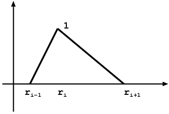
$\displaystyle\rho(r)=\sum_{i}\alpha_{i}\rho_{i}(r)$

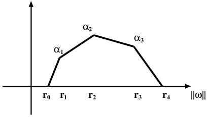
Figure 1: Piecewise linear functions. Left: single basis function. Right: linear combination of three functions. Additional degrees of freedom are fixed by $\rho(r_{0})=\rho(r_{4})=0$.

However, if we remain in the Fourier domain, we can use $\rho(r)$ and sample directly from it. This strategy kills two birds with one stone: we do not need to compute the inverse Fourier transform and we have a readily available sampling distribution at our disposal for the Fastfood expansion coefficients $S_{ii}$. All that is needed is to find an efficient parametrization of $\rho(r)$.

We begin by providing an explicit expression for piecewise linear functions $\rho_{i}$ such that $\rho_{i}(r_{j})=\delta_{ij}$ with discontinuities only at $r_{i-1},r_{i}$ and $r_{i+1}$. In other words, $\rho(r)$ is a ‘hat’ function with its mode at $r_{i}$ and range $[r_{i-1},r_{i+1}]$. It is parametrized as

$$\rho_{i}(r):=\max\left(0,\min\left(1,\frac{r-r_{i-1}}{r_{i}-r_{i-1}},\frac{r_{i}-r}{r_{i+1}-r_{i}}\right)\right)$$

By construction each basis function is piecewise linear with $\rho_{i}(r_{j})=\delta_{ij}$ and moreover $\rho_{i}(r)\geq 0$ for all $r$.

Lemma 2

Denote by $\left\{r_{0},\ldots,r_{n}\right\}$ a sequence of locations with $r_{i}>r_{i-1}$ and $r_{0}=0$. Moreover, let $\rho(r):=\sum_{i}\alpha_{i}\rho_{i}(r)$. Then $\rho(r)\geq 0$ for all $r$ if and only if $\alpha_{i}\geq 0$ for all $i$. Moreover, $\rho(r)$ parametrizes all piecewise linear functions with discontinuities at $r_{i}$.

Now that we have a parametrization we only need to discuss how to draw $\omega$ from $\rho(\left\|\omega\right\|)=\rho(r)$. We have several strategies at our disposal:

• $\rho(r)$ can be normalized explicitly via

  $$\bar{\rho}:=\int_{0}^{\infty}\rho(r)dr=\sum_{i}\frac{\alpha_{i}}{2(r_{i+1}-r_{i-1})}$$

  Since each segment $\rho_{i}$ occurs with probability $\alpha_{i}/(2\bar{\rho}(r_{i+1}-r_{i-1})$ we first sample the segment and then sample from $\rho_{i}$ explicitly by inverting the associated cumulative distribution function (it is piecewise quadratic).

• Note that sampling can induce considerable variance in the choice of locations. An alternative is to invert the cumulative distribution function and pick $m$ locations equidistantly at locations $\frac{i}{m}+\xi$ where $\xi\sim U[0,1/m]$. This approach is commonly used in particle filtering (Doucet et al., 2001). It is equally cheap yet substantially reduces the variance when sampling, hence we choose this strategy.

The basis functions are computed as follows:

  Preprocessing($m,\left\{(\{\alpha_{i}\}_{i=1}^{n},\{r_{i}\}_{i=0}^{n+1},\Sigma)\right\}$)

  Generate random matrices $G,B,\Pi$

  Update scaling $B\leftarrow B\Sigma^{\frac{1}{2}}$

  Sample $S$ from $\rho(\left\|\omega\right\|)$ as above

  Feature Computation($S,G,B,\Pi$)

$$\phi_{1}\leftarrow\cos([SHG\Pi HBx])\text{ and }\phi_{2}\leftarrow\sin([SHG\Pi HBx])$$

The rescaling matrix $\Sigma_{q}$ is introduced to incorporate automatic relevance determination into the model. Like with the Gaussian spectral mixture model, we can use a mixture of piecewise linear radial kernels to approximate any radial kernel. Supposing there are $Q$ components of the piecewise linear $\rho_{q}(r)$ function, we can repeat the proposed algorithm $Q$ times to generate all the required basis functions.

4.5 Fastfood Kernels

The efficiency of Fastfood is partly obtained by approximating Gaussian random matrices with a product of matrices described in section 3.2. Here we propose several expressive and efficient kernel learning algorithms obtained by optimizing the marginal likelihood of the data in Eq. (4.2) with respect to these matrices:

FSARD

The scaling matrix $S$ represents the spectral properties of the associated kernel. For the RBF kernel, $S$ is sampled from a chi-squared distribution. We can simply change the kernel by adjusting $S$. By varying $S$, we can approximate any radial kernel. We learn the diagonal matrix $S$ via marginal likelihood optimization. We combine this procedure with Automatic Relevance Determination of Neal (1998) – learning the scale of the input space – to obtain the FSARD kernel.

FSGBARD

We can further generalize FSARD by additionally optimizing marginal likelihood with respect to the diagional matrices $G$ and $B$ in Fastfood to represent a wider class of kernels.

In both FSARD and FSGBARD the Hadamard matrix $H$ is retained, preserving all the computational benefits of Fastfood. That is, we only modify the scaling matrices while keeping the main computational drivers such as the fast matrix multiplication and the Fourier basis unchanged.

5 Experiments

We evaluate the proposed kernel learning algorithms on many regression problems from the UCI repository. We show that the proposed methods are flexible, scalable, and applicable to a large and diverse collection of data, of varying sizes and properties. In particular, we demonstrate scaling to more than 2 million datapoints (in general, Gaussian processes are intractable beyond $10^{4}$ datapoints); secondly, the proposed algorithms significantly outperform standard exact kernel methods, and with only a few hyperparameters are even competitive with alternative methods that involve training orders of magnitude more hyperparameters. The results are shown in Table 1. All experiments are performed on an Intel Xeon E5620 PC, operating at 2.4GHz with 32GB RAM.

5.1 Experimental Details

To learn the parameters of the kernels, we optimize over the marginal likelihood objective function described in Section 3.1, using LBFGS.

The datasets are divided into three groups: SMALL $n\leq 2000$ and MEDIUM $2,000<n\leq 100,000$ and LARGE $100,000<n\leq 2,000,000$. All methods – RBF, ARD, FSARD, GM, PWL and SSGPR – are tested on each grouping. For SMALL data, we use an exact RBF and ARD kernel. All the datasets are divided into $10$ partitions. Every time, we pick one partition as test data and train all methods on the remaining $1$ partitions. The reported result is based on the averaged RMSE of $10$ partitions.

Methods

RBF and ARD

The RBF kernel has the form $k(x,x^{\prime})=a^{2}\exp\left(-0.5||x-x^{\prime}||^{2}/\ell^{2}\right)$, where $a$ and $\ell$ are signal standard deviation and length-scale (rescale) hyperparameters. The ARD kernel has the form $k(x,x^{\prime})=a^{2}\exp\left(-0.5\sum_{j=1}^{d}(x_{j}-x_{j}^{\prime})^{2}/\ell_{j}^{2}\right)$. ARD kernels use Automatic Relevance Determination (Neal, 1998) to adjust the scales of each input dimension individually. On smaller datasets, with fewer than $n=2000$ training examples, where exact methods are tractable, we use exact Gaussian RBF and ARD kernels with hyperparameters learned via marginal likelihood optimization. Since these exact methods become intractable on larger datasets, we use Fastfood basis function expansions of these kernels for $n>2000$.

GM

For Gaussian Mixtures we compute a mixture of Gaussians in frequency domain, as described in section 4.3. As before, optimization is carried out with regard to marginal likelihood.

PWL

For rotation invariance, we use the novel piecewise linear radial kernels described in section 4.4. PWL has a simple and scalable parametrization in terms of the radius of the spectrum.

SSGPR

Sparse Spectrum Gaussian Process Regression is a kitchen sinks (RKS) based model which individually optimizes the locations of all spectral frequencies (Lázaro-Gredilla et al., 2010). We note that SSGPR is heavily parametrized. Also note that SSGPR is a special case of the proposed GM model if for GM the number of components $Q=m$, and we set all bandwidths to $0$ and weigh all terms equally.

FSARD and FSGBARD

As described in section 4.5, these methods respectively learn the $S$ and $S,G,B$ matrices in the Fastfood representation of section 3.2, through marginal likelihood optimisation (section 4.2).

Initialization

RBF

We randomly pick $max(2000,n/5)$ pairs of data and compute the distance of these pairs. These distances are sorted and we pick the $[0.1:0.2:0.9]$ quantiles as length-scale (aka rescale) initializations. We run $20$ optimization iterations starting with these initializations and then pick the one with the minimum negative log marginal likelihood, and then continue to optimize for $150$ iterations. We initialize the signal and noise standard deviations as $std(y)$ and $std(y)/10$, respectively, where $y$ is the data vector.

ARD

For each dimension of the input, $X_{j}$, we initialize each length-scale parameter as $\ell_{j}=u(max(X_{j})-min(X_{j}))$, where $u\sim\text{Uniform}[0.4,0.8]$. We pick the best initialization from $10$ random restarts of a $20$ iteration optimization run. We multiply the scale by $\sqrt{d}$, the total number of input dimensions.

FSARD

We use the same technique as in ARD to initialize the rescale parameters. We set the $S$ matrix to be $||w||$, where $w$ is a $d$ dimensional random vector with standard Gaussian distribution.

FSGBARD

We initialize $S$ as in FSARD. $B$ is drawn uniformly from $\left\{\pm 1\right\}$ and $G$ from draws of a standard Gaussian distribution.

GM

We use a Gaussian distribution with diagonal covariance matrices to model the spectral density $p(\omega)$. Assuming there are $Q$ mixture components, the scale of each component is initialized to be $std(y)/Q$. We reuse the same technique to initialize the rescale matrices as that of ARD. We initialize the shift $\mu$ to be close to $0$.

PWL

We make use of a special case of a piecewise linear function, the hat function, in the experiments. The hat function is parameterized by $\mu$ and $\sigma$. $\sigma$ controls the width of the hat function and $\mu$ control the distance of the hat function from the origin. We also incorporate ARD in the kernel, and use the same initialization techniques. For the RBF kernel we compute the distance of random pairs and sort these distances. Then we get a distance sample $\lambda$ with a uniform random quantile within $[0.2,0.8]$. $\lambda$ is like the bandwidth of an RBF kernel. Then $\sigma=2/\lambda$ and $\mu=\max\{\sqrt{d-1}-2,0.01\}/\lambda$. We make use of this technique because for RBF kernel, the maximum points is at $\sqrt{d-1}/\lambda$ and the width of the radial distribution is about $2/\lambda$.

SSGPR

For the rescale parameters, we follow the same procedure as for the ARD kernel. We initialize the projection matrix as a random Gaussian matrix.

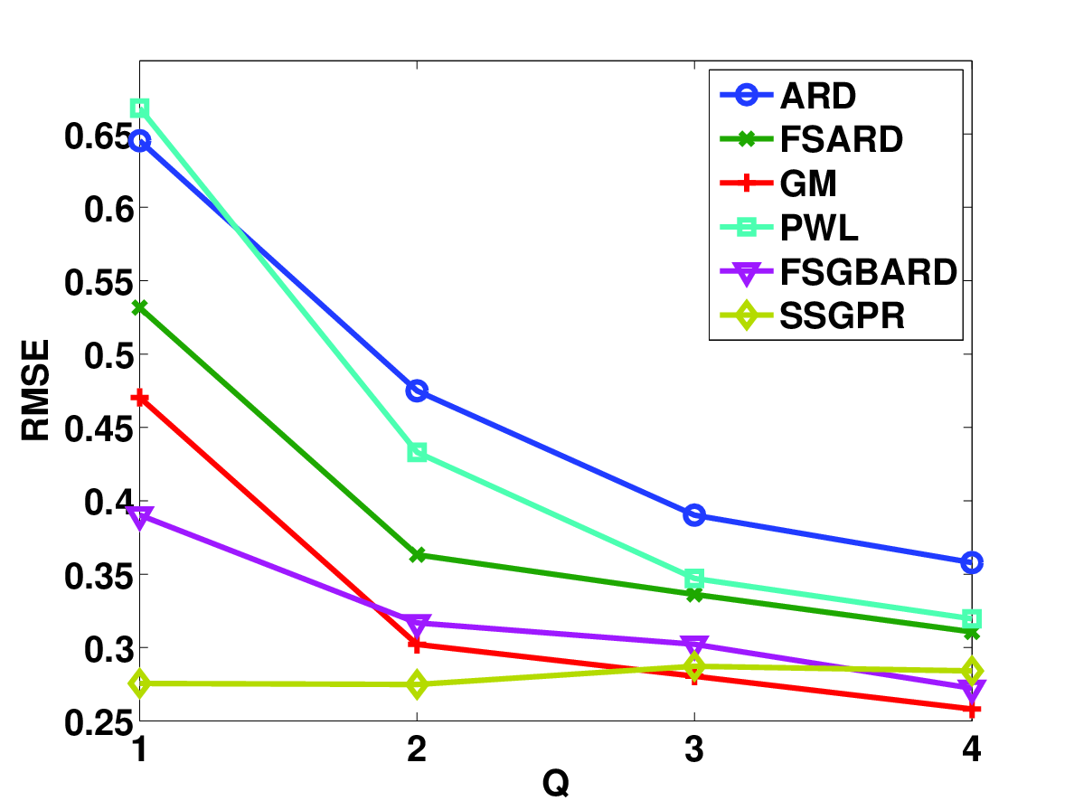
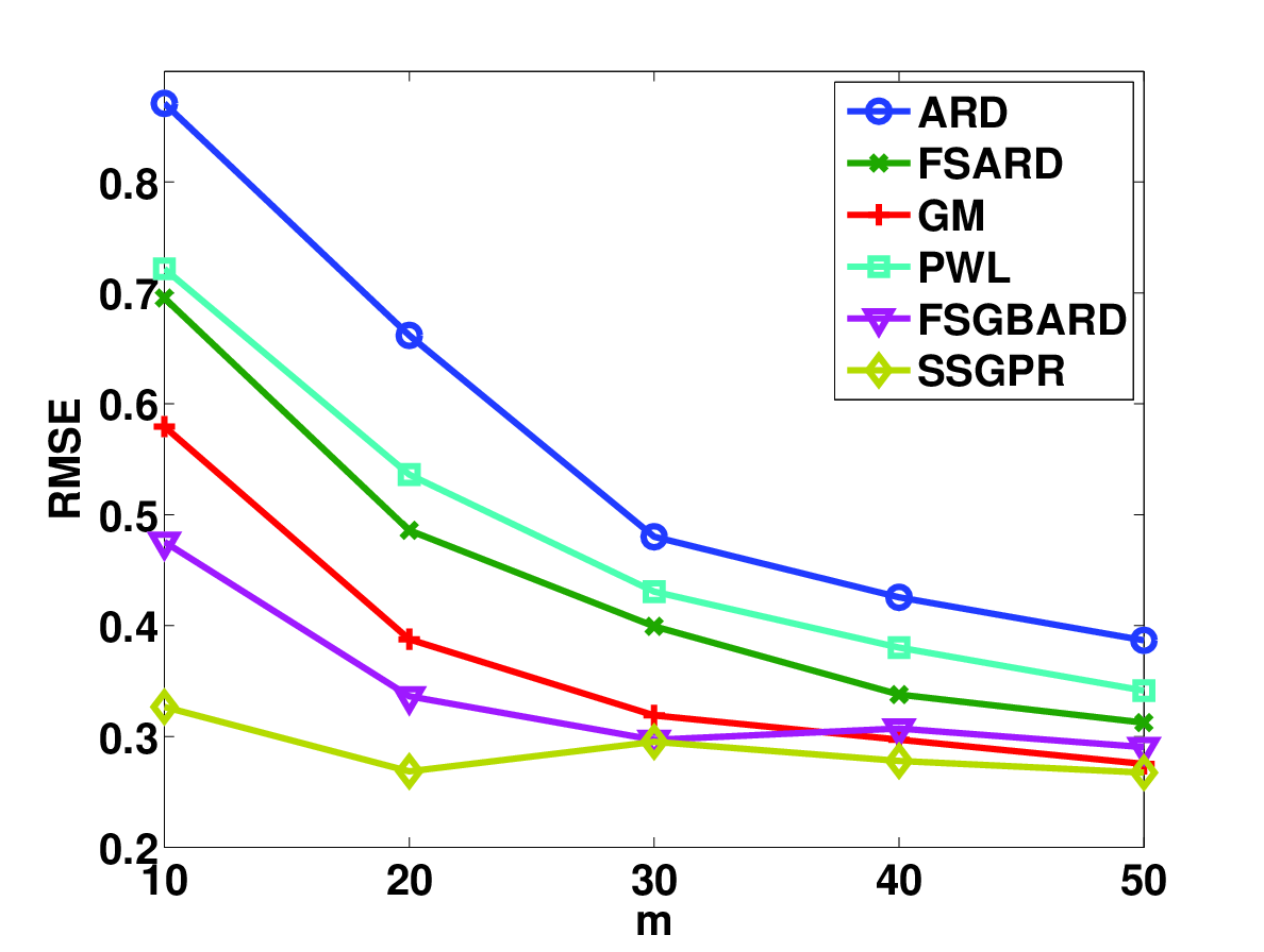
Figure 2: We analyze how the accuracy depends on the number of clusters $Q$ (left) and the number of basis functions $m$ (right). More specifically, for variable $Q$ the number of basis functions per group $m$ is fixed to $32$. For variable $m$ the number of clusters $Q$ is fixed to $2$. FRBF and FARD are Fastfood expansions of RBF and ARD kernels, respectively.

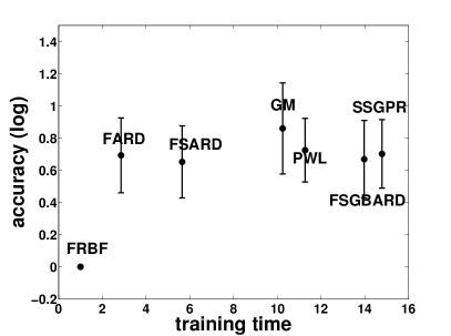
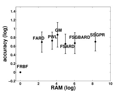
Figure 3: We compare all methods in terms of accuracy, training time (left) and memory (right). To make the methods comparable we compute the accuracy score of a given method as the improvement relative to the baseline (FRBF). That is, we compute $\text{accuracy}_{\text{method}}=\text{RMSE}_{\text{FRBF}}/\text{RMSE}_{\text{method}}$. By construction, FRBF has an accuracy score of $1$, and larger values of accuracy correspond to better algorithms. For runtime and memory we take the reciprocal of the analogous metric, so that a lower score corresponds to better performance. For instance, $\text{time}_{\text{method}}=\text{walltime}_{\text{method}}/\text{walltime}_{\text{FRBF}}$. $\log$ denotes an average of the log scores, across all datasets.

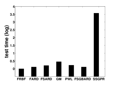
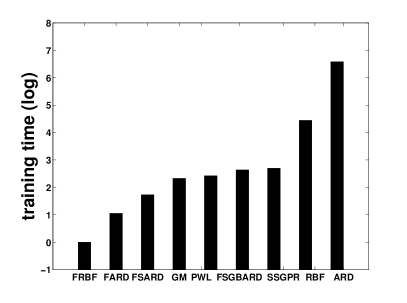
Figure 4: Test time (left) and training time (right), as a function of the method used. This also includes the average log training time for the exact ARD and RBF kernels across the smallest five medium datasets; Note that these methods are intractable on any larger datasets, hence we did not compare them on any of the larger datasets.

Table 1: Comparative RMSE performance on all datasets, with $n$ training points and $d$ the input dimensions. The results are averaged over 10 equal partitions of the data $\pm$ 1 standard deviation. We use exact RBF and ARD kernels on the small datasets, and Fastfood expansions of these kernels on the medium and large datasets. For GM and PWL, we set $Q=5$ and use $m=256$ sample points for each component. For FSARD and SSGPR, we set $m=512$. For medium datasets, we set $Q=3$ and $m=256$ for GM and PWL. On the large datasets 3D Road network and Buzz, GM and PWL use $Q=6$ and $m=16$, and $Q=5$ and $m=8$ for Song and Household electric. All other methods use $Qm$ basis functions. The terms ‘small’, ‘medium’ and ‘large’ are meant to be taken in the context of Gaussian process regression, which is typically intractable for $n>2000$ when kernel learning is taking place.

Datasets	n	d	RBF	ARD	FSARD	GM	PWL	FSGBARD	SSGPR
SMALL:
Challenger	23	4	0.63$\pm$0.26	0.63$\pm$0.26	0.72$\pm$0.34	0.61$\pm$0.27	0.68$\pm$0.28	0.77$\pm$0.39	0.75$\pm$0.38
Fertility	100	9	0.19$\pm$0.04	0.21$\pm$0.05	0.21$\pm$0.05	0.19$\pm$0.05	0.19$\pm$0.05	0.20$\pm$0.04	0.20$\pm$0.06
Slump	103	7	4.49$\pm$2.22	4.72$\pm$2.42	3.97$\pm$2.54	2.99$\pm$1.14	3.45$\pm$1.66	5.40$\pm$2.44	6.25$\pm$3.70
Automobile	159	15	0.14$\pm$0.04	0.18$\pm$0.07	0.18$\pm$0.05	0.15$\pm$0.0311	0.14$\pm$0.03	0.22$\pm$0.08	0.17$\pm$0.06
Servo	167	4	0.29$\pm$0.07	0.28$\pm$0.09	0.29$\pm$0.08	0.27$\pm$0.07	0.28$\pm$0.09	0.44$\pm$0.10	0.38$\pm$0.08
Cancer	194	34	32$\pm$4	35$\pm$4	43$\pm$9	31$\pm$4	35$\pm$6	34$\pm$5	33$\pm$5
Hardware	209	7	0.44$\pm$0.06	0.43$\pm$0.04	0.44$\pm$0.06	0.44$\pm$0.04	0.42$\pm$0.04	0.42$\pm$0.08	0.44$\pm$0.1
Yacht	308	7	0.29$\pm$0.14	0.16$\pm$0.11	0.13$\pm$0.06	0.13$\pm$0.08	0.12$\pm$0.07	0.12$\pm$0.06	0.14$\pm$0.10
Auto MPG	392	7	2.91$\pm$0.30	2.63$\pm$0.38	2.75$\pm$0.43	2.55$\pm$0.55	2.64$\pm$0.52	3.30$\pm$ 0.69	3.19$\pm$0.56
Housing	509	13	3.33$\pm$0.74	2.91$\pm$0.54	3.39$\pm$0.74	2.93$\pm$0.83	2.90$\pm$0.78	4.62$\pm$0.85	4.49$\pm$0.69
Forest fires	517	12	1.39$\pm$0.15	1.39$\pm$0.16	1.59$\pm$0.12	1.40$\pm$0.17	1.41$\pm$0.16	2.64$\pm$0.25	2.01$\pm$0.41
Stock	536	11	0.016$\pm$0.002	0.005$\pm$0.001	0.005$\pm$0.001	0.005$\pm$0.001	0.005$\pm$0.001	0.006$\pm$0.001	0.006$\pm$0.001
Pendulum	630	9	2.77$\pm$0.59	1.06$\pm$0.35	1.76$\pm$0.31	1.06$\pm$0.27	1.16$\pm$0.29	1.22$\pm$0.26	1.09$\pm$0.33
Energy	768	8	0.47$\pm$0.08	0.46$\pm$0.07	0.47$\pm$0.07	0.31$\pm$0.07	0.36$\pm$0.08	0.39$\pm$0.06	0.42$\pm$0.08
Concrete	1,030	8	5.42$\pm$0.80	4.95$\pm$0.77	5.43$\pm$0.76	3.67$\pm$0.71	3.76$\pm$0.59	4.86$\pm$0.97	5.03$\pm$1.35
Solar flare	1,066	10	0.78$\pm$0.19	0.83$\pm$0.20	0.87$\pm$0.19	0.82$\pm$0.19	0.82$\pm$0.18	0.91$\pm$0.19	0.89$\pm$0.20
Airfoil	1,503	5	4.13$\pm$0.79	1.69$\pm$0.27	2.00$\pm$0.38	1.38$\pm$0.21	1.49$\pm$0.18	1.93$\pm$0.38	1.65$\pm$0.20
Wine	1,599	11	0.55$\pm$0.03	0.47$\pm$0.08	0.50$\pm$0.05	0.53$\pm$0.11	0.48$\pm$0.03	0.57$\pm$0.04	0.66$\pm$0.06
MEDIUM:
Gas sensor	2,565	128	0.21$\pm$0.07	0.12$\pm$0.08	0.13$\pm$0.06	0.14$\pm$0.08	0.12$\pm$0.07	0.14$\pm$0.07	0.14$\pm$0.08
Skillcraft	3,338	19	1.26$\pm$3.14	0.25$\pm$0.02	0.25$\pm$0.02	0.25$\pm$0.02	0.25$\pm$0.02	0.29$\pm$0.02	0.28$\pm$0.01
SML	4,137	26	6.94$\pm$0.51	0.33$\pm$0.11	0.26$\pm$0.04	0.27$\pm$0.03	0.31$\pm$0.06	0.31$\pm$0.06	0.34$\pm$0.05
Parkinsons	5,875	20	3.94$\pm$1.31	0.01$\pm$0.00	0.02$\pm$0.01	0.00$\pm$0.00	0.04$\pm$0.03	0.02$\pm$0.00	0.08$\pm$0.19
Pumadyn	8,192	32	1.00$\pm$0.00	0.20$\pm$0.00	0.22$\pm$0.03	0.21$\pm$0.00	0.20$\pm$0.00	0.21$\pm$0.00	0.21$\pm$0.00
Pole Tele	15,000	26	12.6$\pm$0.3	7.0$\pm$0.3	6.1$\pm$0.3	5.4$\pm$0.7	6.6$\pm$0.3	4.7$\pm$0.2	4.3$\pm$0.2
Elevators	16,599	18	0.12$\pm$0.00	0.090$\pm$0.001	0.089$\pm$0.002	0.089$\pm$0.002	0.089$\pm$0.002	0.086$\pm$0.002	0.088$\pm$0.002
Kin40k	40,000	8	0.34$\pm$0.01	0.28$\pm$0.01	0.23$\pm$0.01	0.19$\pm$0.02	0.23$\pm$0.00	0.08$\pm$0.00	0.06$\pm$0.00
Protein	45,730	9	1.64$\pm$1.66	0.53$\pm$0.01	0.52$\pm$0.01	0.50$\pm$0.02	0.52$\pm$0.01	0.48$\pm$0.01	0.47$\pm$0.01
KEGG	48,827	22	0.33$\pm$0.17	0.12$\pm$0.01	0.12$\pm$0.01	0.12$\pm$0.01	0.12$\pm$0.01	0.12$\pm$0.01	0.12$\pm$0.01
CT slice	53,500	385	7.13$\pm$0.11	4.00$\pm$0.12	3.60$\pm$0.09	2.21$\pm$0.06	3.35$\pm$0.08	2.56$\pm$0.12	0.59$\pm$0.07
KEGGU	63,608	27	0.29$\pm$0.12	0.12$\pm$0.00	0.12$\pm$0.00	0.12$\pm$0.00	0.12$\pm$0.00	0.12$\pm$0.00	0.12$\pm$0.00
LARGE:
3D road	434,874	3	12.86$\pm$0.09	10.91$\pm$0.05	10.29$\pm$0.12	10.34$\pm$0.19	11.26$\pm$0.22	9.90$\pm$0.10	10.12$\pm$0.28
Song	515,345	90	0.55$\pm$0.00	0.49$\pm$0.00	0.47$\pm$0.00	0.46$\pm$0.00	0.47$\pm$0.00	0.46$\pm$0.00	0.45$\pm$0.00
Buzz	583,250	77	0.88$\pm$0.01	0.59$\pm$0.02	0.54$\pm$0.01	0.51$\pm$0.01	0.54$\pm$0.01	0.52$\pm$0.01	0.54$\pm$0.01
Electric	2,049,280	11	0.23$\pm$0.00	0.12$\pm$0.12	0.06$\pm$0.01	0.05$\pm$0.00	0.07$\pm$0.04	0.05$\pm$0.00	0.05$\pm$0.00

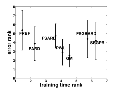
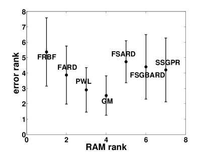
Figure 5: To assess the relative performance of the algorithms with respect to another, we compare their relative error rank as a function of training time (left) and memory footprint (right).

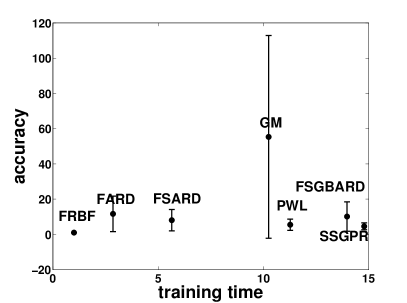
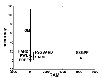
Figure 6: Accuracy of the algorithms as a function of training time (left) and memory (right).

We use the same number of basis functions for all methods. We use $Q$ to denote the number of components in GM and PWL and $m$ to denote the number of basis functions in each component. For all other methods, we use $Qm$ basis functions. For the largest datasets in Table 1 we favoured larger values of $Q$, as the flexibility of having more components $Q$ in GM and PWL becomes more valuable when there are many datapoints; although we attempted to choose sensible $Q$ and $m$ combinations for a particular model and number of datapoints $n$, these parameters were not fine tuned. We choose $Qm$ to be as large as is practical given computational constraints, and SSGPR is allowed a significantly larger parametrization.

Indeed SSPGR is allowed $Qmd+2$ free parameters to learn, and we set $Q\ll m$. This setup gives SSGPR a significant advantage over our proposed models. However, we wish to emphasize that the GM, PWL, and FSGBARD models are competitive with SSGPR, even in the adversarial situation when SSGPR has many orders of magnitude more free parameters than GM or PWL. For comparison, the RBF, ARD, PWL, GM, FSARD and FSGBARD methods respectively require $3,d+2,Q(d+3)+1,Q(2d+1)+1,Qm+d+2,$ and $3Qm+d+2$ hyperparameters.

Gaussian processes are most commonly implemented with exact RBF and ARD kernels, which we run on the smaller ($n<2000$) datasets in Table 1, where the proposed GM and PWL approaches generally perform better than all alternatives. On the larger datasets, exact ARD and RBF kernels are entirely intractable, so we compare to Fastfood expansions. That is, GM and PWL are both more expressive and profoundly more scalable than exact ARD and RBF kernels, far and above the most popular alternative approaches.

In Figure 2 we investigate how RMSE performance changes as we vary $Q$ and $m$. The GM and PWL models continue to increase in performance as more basis functions are used. This trend is not present with SSGPR or FSGBARD, which unlike GM and PWL, becomes more susceptible to over-fitting as we increase the number of basis functions. Indeed, in SSGPR, and in FSGBARD and FSARD to a lesser extent, more basis functions means more parameters to optimize, which is not true with the GM and PWL models.

To further investigate the performance of all methods, we compare each of the seven tested methods over all experiments, in terms of average normalised log predictive accuracy, training time, testing time, and memory consumption, shown in Figures 3 and 4 (higher accuracy scores and lower training time, test time, and memory scores, correspond to better performance). Despite the reduced parametrization, GM and PWL outperform all alternatives in accuracy, yet require similar memory and runtime to the much less expressive FARD model, a Fastfood expansion of the ARD kernel. Although SSGPR performs third best in accuracy, it requires more memory, training time, testing runtime (as shown in Fig 4), than all other models. FSGBARD performs similar in accuracy to SSGPR, but is significantly more time and memory efficient, because it leverages a Fastfood representation. For clarity, we have so far considered log plots. If we view the results without a log transformation, as in Fig 6 (supplement) we see that GM and SSGPR are outliers: on average GM greatly outperforms all other methods in predictive accuracy, and SSGPR requires profoundly more memory than all other methods.

6 Discussion

Kernel learning methods are typically intractable on large datasets, even though their flexibility is most valuable on large scale problems. We have introduced a family of flexible, scalable, general purpose and lightly parametrized kernel methods, which learn the properties of groups of spectral frequencies in Fastfood basis function expansions. We find, with a minimal parametrization, that the proposed methods have impressive performance on a large and diverse collection of problems – in terms of predictive accuracy, training and test runtime, and memory consumption. In the future, we expect additional performance and efficiency gains by automatically learning the relative numbers of spectral frequencies to assign to each group.

In short, we have shown that we can have kernel methods which are simultaneously scalable and expressive. Indeed, we hope that this work will help unify efforts in enhancing scalability and flexibility for kernel methods. In a sense, flexibility and scalability are one and the same problem: we want the most expressive methods for the biggest datasets.

References

- Doucet et al. [2001] A. Doucet, N. de Freitas, and N. Gordon. Sequential Monte Carlo Methods in Practice. Springer-Verlag, 2001.
- Halko et al. [2009] N. Halko, P.G. Martinsson, and J. A. Tropp. Finding structure with randomness: Stochastic algorithms for constructing approximate matrix decompositions, 2009. URL http://arxiv.org/abs/0909.4061. oai:arXiv.org:0909.4061.
- Kimeldorf and Wahba [1970] G. S. Kimeldorf and G. Wahba. A correspondence between Bayesian estimation on stochastic processes and smoothing by splines. Annals of Mathematical Statistics, 41:495–502, 1970.
- Lázaro-Gredilla et al. [2010] M. Lázaro-Gredilla, J. Quiñonero-Candela, C. E. Rasmussen, and A. R. Figueiras-Vidal. Sparse spectrum gaussian process regression. The Journal of Machine Learning Research, 99:1865–1881, 2010.
- Le et al. [2013] Q.V. Le, T. Sarlos, and A. J. Smola. Fastfood — computing hilbert space expansions in loglinear time. In International Conference on Machine Learning, 2013.
- Lu et al. [2014] Z. Lu, M. May, K. Liu, A.B. Garakani, Guo D., A. Bellet, L. Fan, M. Collins, B. Kingsbury, M. Picheny, and F. Sha. How to scale up kernel methods to be as good as deep neural nets. Technical Report 1411.4000, arXiv, November 2014. http://arxiv.org/abs/1411.4000.
- Mercer [1909] J. Mercer. Functions of positive and negative type and their connection with the theory of integral equations. Philos. Trans. R. Soc. Lond. Ser. A Math. Phys. Eng. Sci., A 209:415–446, 1909.
- Neal [1998] R. M. Neal. Assessing relevance determination methods using delve. In C. M. Bishop, editor, Neural Networks and Machine Learning, pages 97–129. Springer, 1998.
- Ong et al. [2003] C. S. Ong, A. J. Smola, and R. C. Williamson. Hyperkernels. In S. Thrun S. Becker and K. Obermayer, editors, Advances in Neural Information Processing Systems 15, pages 478–485. MIT Press, Cambridge, MA, 2003.
- Rahimi and Recht [2008] A. Rahimi and B. Recht. Random features for large-scale kernel machines. In J.C. Platt, D. Koller, Y. Singer, and S. Roweis, editors, Advances in Neural Information Processing Systems 20. MIT Press, Cambridge, MA, 2008.
- Rahimi and Recht [2009] A. Rahimi and B. Recht. Weighted sums of random kitchen sinks: Replacing minimization with randomization in learning. In Neural Information Processing Systems, 2009.
- Rasmussen and Williams [2006] C. E. Rasmussen and C. K. I. Williams. Gaussian Processes for Machine Learning. MIT Press, Cambridge, MA, 2006.
- Schoenberg [1942] I. Schoenberg. Positive definite functions on spheres. Duke Math. J., 9:96–108, 1942.
- Schölkopf et al. [2001] B. Schölkopf, R. Herbrich, and A. J. Smola. A generalized representer theorem. In D. P. Helmbold and B. Williamson, editors, Proc. Annual Conf. Computational Learning Theory, number 2111 in Lecture Notes in Comput. Sci., pages 416–426, London, UK, 2001. Springer-Verlag.
- Silverman [1986] B. W. Silverman. Density Estimation for Statistical and Data Analysis. Monographs on statistics and applied probability. Chapman and Hall, London, 1986.
- Williams [1998] C. K. I. Williams. Prediction with Gaussian processes: From linear regression to linear prediction and beyond. In M. I. Jordan, editor, Learning and Inference in Graphical Models, pages 599–621. Kluwer Academic, 1998.
- Wilson and Adams [2013] A. G. Wilson and R. P. Adams. Gaussian process kernels for pattern discovery and extrapolation. In Proceedings of the 30th International Conference on Machine Learning, 2013.
- Wilson [2014] A.G. Wilson. Covariance Kernels for Fast Automatic Pattern Discovery and Extrapolation with Gaussian Processes. PhD thesis, University of Cambridge, 2014.
- Wilson et al. [2014] A.G. Wilson, E. Gilboa, A. Nehorai, and J.P. Cunningham. Fast kernel learning for multidimensional pattern extrapolation. In Advances in Neural Information Processing Systems, 2014.