Qualitative Aspects of the Solutions of a Mathematical Model for the Dynamic Analysis of the Reversible Chemical Reaction $\mbox{SO}_{2\,(\mathrm{g})}\,+\,\frac{1}{2}\,\mbox{O}_{2\,(\mathrm{g})}\,\rightleftharpoons\,\mbox{SO}_{3\,(\mathrm{g})}$ in a Catalytic Reactor

Abstract

We present some qualitative aspects concerning the solution to the mathematical model describing the dynamical behavior of the reversible chemical reaction $\mbox{SO}_{2\,(\mathrm{g})}\,+\,\frac{1}{2}\,\mbox{O}_{2\,(\mathrm{g})}\,\rightleftharpoons\,\mbox{SO}_{3\,(\mathrm{g})}$ carried out in a catalytic reactor used in the process of sulfuric acid production.

PACS numbers:

I Introduction

The production of most industrially important chemicals involves catalysis. Catalysis is relevant to many aspects of environmental science, e.g. the catalytic converter in automobiles and the dynamics of the ozone hole. Catalytic reactions are preferred in environmentally friendly green chemistry due to the reduced amount of waste generated, as opposed to stoichiometric reactions in which all reactants are consumed and more collaterals products are formed. Particularly, the oxidation of sulfur dioxide to sulfur trioxide using oxygen or air and a suitable catalyst such as vanadium pentoxide is well known for the sulfuric acid production. In this sense, the idea that the performance of these continuous catalytic processes under invariable conditions is highly efficient has gained great popularity, among chemical engineers that design catalytic reactors where the reaction will be carried out ca . However, very often the optimal conditions of the process can be achieved with the unsteady-state operation and the steady-state operation will be a particular case of the unsteady-state conditions. Unsteady-state operation broadens the possibilities to form the profiles of the catalyst states, concentrations, and temperatures in reactors, thus providing more favorable conditions for the process performance mm . Research work like this involve many areas of chemistry and physical-chemistry, but mathematical modeling is an important tool for rapid and reliable reactor development and design carberry . The models are built from the basic studies of the reaction mechanism and kinetics, the transfer processes, and the interactions within the system. A detailed understanding of the elementary processes enables the construction of powerful and complex models for dynamic and steady-state simulation. With the aid of experimentally determined parameter values we can develop new processes or improve existing ones using dynamical simulations based on its mathematical models bales .

In this work, we present a mathematical model for the dynamical analysis of the reversible chemical reaction associated to the oxidation of sulfur dioxide to sulfur trioxide using oxygen in presence of the vanadium pentoxide catalyst, and we study some qualitative aspects concerning its solution as a previous step for the simulation of the catalytic reactor where the reaction will be carried out.

This paper is organized as follows. In Section II we present the mathematical model formulated as a problem of Cauchy or initial conditions for the state variables that they define to the studied catalytic system, using as reference a model presented in ctacv . In Section III we begin the qualitative study of the mathematical model demonstrating that this is a well-posed problem; in addition we present the characteristics of the set of steady-state. Next, Section IV is devoted to the study the solutions of the dynamics states for the system, we present the qualitative aspects concerning the behavior when the operation time is very long. In Section V we present a brief discussion from the physicochemical point of view and we finalize with the conclusions of this research in Section VI.

II Mathematical model

II.1 Description of the catalytic system

The studied catalytic system was the oxidation of sulfur dioxide (SO₂) to sulfur trioxide (SO₃) in presence of the vanadium pentoxide catalyst (Vn₂O₅). The stoichiometric equation is:

$$\mbox{SO}_{2\,(\mbox{g})}\,+\,\frac{1}{2}\,\mbox{O}_{2\,(\mbox{g})}\,\rightleftharpoons\,\mbox{SO}_{3\,(\mbox{g})}.$$ (1)

This reaction is exothermic in the forward direction, denoted by $\rightharpoonup$, and endothermic in the reverse direction, denoted by $\leftharpoondown$. Also, the reaction is a homogenous mixture, its reactans and products are in gaseous phase relative to the conditions of operation in the bed of the catalytic reactor. The speed of this reaction has been widely studied and the expression that suits best is the Eklund’s equation ( see mm ):

$$r_{\mbox{SO}_{2}}=k\sqrt{\frac{p_{\mbox{SO}_{2}}}{p_{\mbox{SO}_{3}}}}\left[p_{\mbox{O}_{2}}-\left(\frac{p_{\mbox{SO}_{3}}}{p_{\mbox{SO}_{2}}k_{p}}\right)^{2}\right],$$ (2)

where $r_{\mbox{SO}_{2}}$ is the reaction rate referred to the SO₂ ($\mbox{mol SO}_{2}/\mbox{s$\cdot$gr of the catalyst}$), $p_{i}$ is the partial pressure (atm) of the $i$-th component ($i=\mbox{SO}_{2},\mbox{ SO}_{3},\mbox{ O}_{2}$), $k$ is the kinetic coefficient of reaction rate and $k_{p}$ the coefficient of chemical equilibrium, both as a function of the temperature (for more details, see ca and fo ).

II.2 Formulation of the mathematical model

For the sake of simplicity, we consider a fixed volume element of catalyst bed, with cylindrical geometry of finite length $L$ and radius $R$, in which the reaction is carried out. We assume that gradients of concentration and temperature in the radial direction ($0\leq r\leq R$) of the catalyst bed do not exist. These gradients are more noticeable in the longitudinal direction ($0\leq z\leq L$), but this spatial variation is not considered for the dynamic study that we will address in this work. Finally, we consider only the variation of the concentration and temperature with respect to the time, and we assume that the changes in the total pressure of the system with respect to time are negligibles at each bed’s output, therefore a balance of momentum was not needed.

The complete problem of interest, obtained by a dynamic balance of matter and caloric energy, is described by the following equations:

$$\frac{dX_{\mbox{A}}(t)}{dt} = \frac{-r_{\mbox{A}}\left(1+\epsilon X_{\mbox{A}}(t)\right)\left(1-\phi\right)\rho_{c}}{C_{\mbox{A}_{0}}},$$

$$\frac{dT(t)}{dt} = \frac{-r_{\mbox{A}}\left(1+\epsilon X_{\mbox{A}}(t)\right)\left(1-\phi\right)\rho_{c}\left(-\Delta Hr\right)}{C_{\mbox{A}_{0}}\left(\sum_{i}\theta_{i}Cp_{i}+X_{\mbox{A}}(t)\Delta Cp\right)+C_{\mbox{I}}Cp_{\mbox{I}}},$$

with the initial data $X_{\mbox{A}}(0)=X_{\mbox{A}_{0}}$ and $T(0)=T_{0}$ for the state variables $X_{A}$ and $T$ respectively. The subscript (A) was used to denote component SO₂ and subscript (I) to denote inert present in the mixture such as bimolecular nitrogen. Therefore, $X_{\mbox{A}}$ represents the molar conversion of the $\mathrm{SO}_{2}$ in the mixture, $r_{\mbox{A}}=f(X_{\mbox{A}},T)$ is the Eklund’s expression written in terms of the molar conversion and of the temperature $T$ of the system. On the other hand $\epsilon$, $\phi$, $\rho_{c}$, $C_{\mbox{A}_{0}}$, $Cp_{i}$, $\theta_{i}$, $\Delta Cp$, $C_{\mbox{I}}$ and $Cp_{\mbox{I}}$ are (constant) given physical parameters. This model is complemented with the following relations:

• Coefficient of chemical equilibrium

  $$k_{p}=\exp{\left(\frac{11829\text{.}44}{T}-11\text{.}24\right)}.$$ (4)

• Kinetic coefficient of reaction rate

  $$k=\exp{\left(\frac{-97782\text{.}22}{T}-110\ln{(1\text{.}8T)}+912\text{.}8\right)}$$ (5)

• Heat of reaction

  $$\Delta H_{r}=34923\text{.}286-65\text{.}395T+0\text{.}0725T^{2}.$$ (6)

II.3 Abstraction of the mathematical model

We begin redefining the two state variables (conversion of the SO₂ and temperature of the system) as follows:

$$u_{1}=u_{1}(t)=X_{\mbox{A}}(t)\,\,\mbox{ and }\,\,u_{2}=u_{2}(t)=T(t),$$

such that, for all time $t\in[0,+\infty)$, $\mathbf{u}(t)=\left(u_{1}(t),u_{2}(t)\right)$ is the vectorial function of the two state variables to determine in the subset $\bar{\Omega}\subset\mathbb{R}^{2}$ given by

$$\bar{\Omega}=[0,u_{1}^{\ast}]\times[u_{2}^{-},u_{2}^{+}],$$

with $u_{1}^{\ast}=1-\delta$ for $0<\delta<1$, and where $u_{2}^{-}$ and $u_{2}^{+}$, respectively, are taken as

$$u_{2}^{-}=\min\limits_{t\in[0,+\infty)}\{0<T(t)<\infty\}\hskip 8.5359pt\mbox{and}\hskip 8.5359ptu_{2}^{+}=\max\limits_{t\in[0,+\infty)}\{0<T(t)<\infty\}.$$ (7)

The right side of each EDO in (LABEL:eq3) is a real valued function defined on $\bar{\Omega}$:

$$f_{1}(\mathbf{u})=\beta_{1}r_{A}(\mathbf{u})g_{1}(u_{1})\hskip 8.5359pt\mbox{and}\hskip 8.5359ptf_{2}(\mathbf{u})=f_{1}(\mathbf{u})g_{2}(\mathbf{u}),$$

where

$$g_{1}(u_{1})=1+\epsilon u_{1},\hskip 8.5359ptg_{2}(\mathbf{u})=\frac{b_{1}+b_{2}u_{2}+b_{3}u_{2}^{2}}{\beta_{2}+\beta_{3}u_{1}}\hskip 8.5359pt\mbox{and}\hskip 8.5359ptr_{A}(\mathbf{u})=K_{1}(u_{2})K_{2}(u_{1})K_{3}(\mathbf{u}),$$

with

$$K_{1}(u_{2})=\exp{\left(\frac{a_{1}}{u_{2}}+a_{2}\ln{(a_{3}u_{2})}+a_{4}\right)},\hskip 8.5359ptK_{2}(u_{1})=\sqrt{\frac{1-u_{1}}{\theta_{c}+u_{1}}},$$

$$K_{3}(\mathbf{u})=L_{1}(u_{1})-L_{2}(u_{1})L_{3}(u_{2}).$$

For $K_{3}$, functions $L_{1}$, $L_{2}$ and $L_{3}$ are given by:

$$L_{1}(u_{1})=\frac{a_{5}-a_{6}u_{1}}{g_{1}(u_{1})},\hskip 8.5359ptL_{2}(u_{1})=\left(\frac{\theta_{c}+u_{1}}{1-u_{1}}\right)^{2}\hskip 8.5359pt\mbox{and}\hskip 8.5359ptL_{3}(u_{2})=\frac{1}{\left(\exp{\left(\frac{a_{7}}{u_{2}}+a_{8}\right)}\right)^{2}}.$$

Here, $\beta_{1}$, $\beta_{2}$, $\beta_{3}$, $\theta_{c}$, $a_{3}$, $a_{4}$, $a_{5}$, $a_{6}$, $a_{7}$, $b_{1}$ and $b_{3}$ are constant strictly positive; $\epsilon$, $a_{1}$, $a_{2}$, $a_{8}$, $b_{2}$ and $b_{4}$ are constant strictly negative. For some of these constants, the physicochemical behavior of the system provides the following restrictions:

$$\beta_{2} > \beta_{3}>\beta_{1},$$

$$0 < \theta_{c}\ll 1,$$

$$a_{7}>a_{4} > a_{3}>a_{5}>a_{6},$$

$$a_{8} > a_{2}>a_{1},$$

$$b_{1} > b_{3},$$

$$\left|\epsilon\right| < 1,$$

$$-1/\epsilon \gg 1,$$

$$b_{2}^{2} \ll 4b_{3}b_{1}.$$

With all the above, the functions $f_{1}$ and $f_{2}$ define the components of a vectorial field (of directions):

$$\mathbf{f}:\bar{\Omega}\subseteq\mathbb{R}^{2}\rightarrow\mathbb{R}^{2}$$ (8)

and the mathematic model (LABEL:eq3)is rewritten as the problem of Cauchy, or initial conditions, for two nonlinear ordinary differential equations: given the vector $\mathbf{u}^{0}\in\bar{\Omega}$, to find $\mathbf{u}\in\bar{\Omega}$ solution of

$$\frac{d\mathbf{u}(t)}{dt} = \mathbf{f}(\mathbf{u}(t)),\hskip 8.5359pt\forall t\in[0,+\infty),$$

$$\mathbf{u}(0) = \mathbf{u}^{0}.$$

III Solutions of the mathematical model

III.1 Solutions of steady-state

The dynamic analysis of a chemical reaction by means of a mathematical model begins by the determination of the stationary states. For the reaction studied in this paper the steady-states are given by the following subset:

$$\Gamma=\left\{\mathbf{u}^{e}=(u^{e}_{1},u^{e}_{2})\in\bar{\Omega};\hskip 5.69046pt\mathbf{f}(\mathbf{u}^{e})=\mathbf{0},\hskip 2.84544ptu_{1}^{e}\in[0,u_{1}^{\ast}],\hskip 2.84544pt\mbox{whit}\hskip 5.69046ptu_{1}^{e}\neq-\frac{1}{\epsilon},u_{2}^{e}=h(u_{1}^{e})\right\},$$

where $h:[0,u_{1}^{\ast}]\rightarrow\mathbb{R}$ is defined as

$$h(u_{1})=\frac{a_{7}}{\ln{\biggl{(}\sqrt{\frac{L_{2}(u_{1})}{L_{1}(u_{1})}}\biggr{)}}-a_{8}},$$

for which it is easily verifiably that $\lim\limits_{u_{1}\rightarrow 1}{h(u_{1})=0}$ and thus, $u_{2}^{-}=h(u_{1}^{\ast})$ and $u_{2}^{+}=h(0)$.

The subset previously defined divides the set $\Omega$ into two simply connected subdomains $\Omega_{1}$ and $\Omega_{2}$:

$$\Omega_{1} = \{\mathbf{u}=(u_{1},u_{2});\hskip 5.69046ptu_{2}^{-}<u_{2}<u_{2}^{e},\hskip 2.84544pt\forall u_{1}\in(0,u_{1}^{\ast})\},$$

$$\Omega_{2} = \{\mathbf{u}=(u_{1},u_{2});\hskip 5.69046ptu_{2}^{e}<u_{2}<u_{2}^{+},\hskip 2.84544pt\forall u_{1}\in(0,u_{1}^{\ast})\};$$

indeed $\Gamma=\bar{\Omega}_{1}\cap\bar{\Omega}_{2}$. Figure 1 illustrates the continuous $\Gamma$ of steady-states and the subsets $\Omega_{1}$ and $\Omega_{2}$.

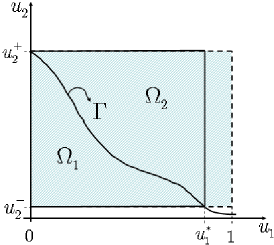
Figure 1: Continuous of steady-states $\Gamma$ and subsets $\Omega_{1}$ and $\Omega_{2}$

III.2 Existence and uniqueness of the solutions of dynamic state

The global existence and uniqueness of the solutions of dynamic state for the problem (LABEL:eq9.1), are a direct consequence of the associated global Lipschitz property to the vectorial field $\mathbf{f}$ on $\Omega\cup\Gamma$. Simultaneously, this property is a direct consequence of the existence and boundedness of the partials drivative $\partial f_{i}/\partial u_{j}$, $i,j=1,2$, on $\Omega\cup\Gamma$ (see ti , cl , ah and ii ), associated to the component functions (scalar fields) $f_{i}$. This is the objective of the following proposition.

Proposition 1.

For each scalar field $f_{i}:\Omega\cup\Gamma\rightarrow\mathbb{R}$, $i=1,2$, the partial derivative $\partial f_{i}/\partial u_{j}$, $i,j=1,2$, exist and is bounded on $\Omega\cup\Gamma$.

Proof. Thanks to the structure of each scalar field $f_{i}$ there exists $\partial f_{i}/\partial u_{j}$ for $i,j=1,2$. Indeed, we have:

$$\frac{\partial f_{1}}{\partial u_{1}} = \beta_{1}\left[g_{1}\frac{\partial r_{A}}{\partial u_{1}}+\epsilon r_{A}\right],$$

$$\frac{\partial f_{1}}{\partial u_{2}} = \beta_{1}g_{1}\frac{\partial r_{A}}{\partial u_{2}};$$

$$\frac{\partial f_{2}}{\partial u_{1}} = g_{2}\frac{\partial f_{1}}{\partial u_{1}}+f_{1}\frac{\partial g_{2}}{\partial u_{1}},$$

$$\frac{\partial f_{2}}{\partial u_{2}} = g_{2}\frac{\partial f_{1}}{\partial u_{2}}+f_{1}\frac{\partial g_{2}}{\partial u_{2}}.$$

Finally, as all the previous derivative are functions composed of continuous and bounded elementary functions on $\Omega\cup\Gamma$, then these derivatives also are continuous and bounded functions on $\Omega\cup\Gamma$ pz ; rb , i.e, for all well-know and fixed physicochemical parameters, there exists a constant $C^{i}_{j}$, for $i,j=1,2$, depending only on $\delta$ such that

$$\left|\frac{\partial f_{i}}{\partial u_{j}}\right|<C_{j}^{i}.$$

Indeed, taking the absolute-value in both members from the expressions (LABEL:eq18) and (LABEL:eq19) we have:

$$C^{1}_{1}=\frac{\beta_{1}M_{1}}{\theta^{{}^{1/2}}}\left[\frac{\Lambda_{1}(\theta_{c},\delta)\Lambda_{2}(\theta_{c},\delta)}{\biggl{(}\exp\biggl{(}\frac{a_{7}}{u_{2}^{+}}+a_{8}\biggr{)}\biggr{)}^{2}}+\frac{1}{|1+\epsilon(1-\delta)|}\biggl{(}(\Lambda_{3}(\theta_{c},\delta)+1)a_{5}+\frac{a_{6}+a_{5}}{|1+\epsilon(1-\delta)|}\biggr{)}\right],$$

$$C_{2}^{1}=\frac{\beta_{1}M_{1}}{\theta_{c}^{{}^{1/2}}(u_{2}^{-})^{2}}\left[\frac{\delta^{2}\Lambda_{1}^{2}(\theta_{c},\delta)(|a_{2}|u_{2}^{-}+a_{1}+2a_{7})}{\biggl{(}\exp\biggl{(}\frac{a_{7}}{u_{2}^{+}}+a_{8}\biggr{)}\biggr{)}^{2}}+\frac{a_{5}(|a_{2}|u_{2}^{-}+a_{1})}{|1+\epsilon(1-\delta)|}\right];\hskip 170.71652pt$$

$$C_{1}^{2}=\biggl{(}\frac{b_{1}+|b_{2}|u_{2}^{-}+b_{3}(u_{2}^{+})^{2}}{\beta_{2}}\biggr{)}\left[C_{1}^{1}\hskip 170.71652pt\right.$$

$$\hskip 142.26378pt\left.+\frac{\beta_{1}\beta_{3}M_{1}}{\beta_{2}\theta_{c}^{{}^{1/2}}}\left(\frac{\delta^{2}\Lambda_{1}^{2}(\theta_{c},\delta)}{\left(\exp\left(\frac{a_{7}}{u_{2}^{+}}+a_{8}\right)\right)^{2}}+\frac{a_{5}}{|1+\epsilon(1-\delta)|}\right)\right],$$

$$C_{2}^{2}=\biggl{(}\frac{b_{1}+|b_{2}|u_{2}^{-}+b_{3}(u_{2}^{+})^{2}}{\beta_{2}}\biggr{)}C_{2}^{1}\hskip 170.71652pt$$

$$\hskip 99.58464pt+\frac{\beta_{1}M_{1}(|b_{2}|+2b_{3}u_{2}^{+})}{\beta_{2}\theta_{c}^{{}^{1/2}}}\left(\frac{\delta^{2}\Lambda_{1}^{2}(\theta_{c},\delta)}{\left(\exp\left(\frac{a_{7}}{u_{2}^{+}}+a_{8}\right)\right)^{2}}+\frac{a_{5}}{|1+\epsilon(1-\delta)|}\right),$$

where

$$\Lambda_{1}(\delta) = \frac{\theta_{c}-\delta+1}{\delta^{2}};$$

$$\Lambda_{2}(\delta) = \frac{4\theta_{c}\delta^{{}^{1/2}}(1+\theta_{c})+\delta(\theta_{c}+1)(\theta_{c}-\delta+1)+2\theta_{c}\delta^{{}^{3/2}}(\theta_{c}-\delta+1)}{2\theta_{c}\delta^{{}^{1/2}}};$$

$$\Lambda_{3}(\delta) = \frac{\theta_{c}+1}{2\theta_{c}\delta^{{}^{1/2}}}.$$

$\blacksquare$

The following corollary is a consequence of the above Proposition.

Corollary 1.

Each scalar field $f_{i}$, $i=1,2$, is a function of class $\mathcal{C}^{1}(\Omega\cup\Gamma,\mathbb{R})$.

By this Corollary and classic results of continuous and differentiable functions (see ii ), the following proposition is automatic.

Proposition 2.

The scalar field $f_{i}:\Omega\cup\Gamma\rightarrow\mathbb{R}$, $i=1,2$, satisfies a global Lipschitz condition on $\Omega\cup\Gamma$.

Proposition 2 guarantees that (LABEL:eq9.1) is a well-posed problem. Therefore, we finalize this section formulating the following result.

Proposition 3.

The problem (LABEL:eq9.1) has a unique solution $\mathbf{u}\in\mathcal{C}^{1}([0,+\infty),\Omega\cup\Gamma)$ that verifies the given initial conditions $\mathbf{u}^{0}(t_{0})\in\Omega\cup\Gamma$ for all $t_{0}\in[0,+\infty)$.

IV Behavior of the solutions of dynamic state for long times

Great part of the dynamic analysis of the reactive systems centers its attention in predicting what will happen to the state variables when these evolve from an initial time $t_{0}\geq 0$ or equivalent, to establish the dynamic behavior of the system for all times $t>t_{0}$. Particularly it is of interest for the engineer to know how the system will behave when time becomes large, because this will allow him to determine operation’s ranks by means of automatic control systems designed and implemented consistently with the desired state. Typically, the state desired at the industrial level corresponds with a steady-state, therefore, from the mathematical point of view we are concerned to find out solutions $\mathbf{u}(t)$ of the model (LABEL:eq9.1) that start at an initial value $\mathbf{u}^{0}$ near or distant a steady-state $\mathbf{u}^{e}\in\Gamma$, will tend to this steady-state or another when time $t$ tends to infinite. For this reason, in this work we combine our analysis with some reported numerical simulations in ctacv that were generated by means of a computer code based on the method of Runge-Kutta to fourth order.

Figures 2 and 3 are the simulations of four solutions $u_{i}=u_{i}(t)$, $i=1,2$, that start from four different initial states $u_{i}^{0}=u_{i}(0)$, $i=1,2$, and Figure 4 illustrates a phase portrait where the evolution of the dynamic states defined by the pair $\mathbf{u}(t)=(u_{1}(t),u_{2}(t))\in\bar{\Omega}$, for all time $t>t_{0}$, can be demonstrated.

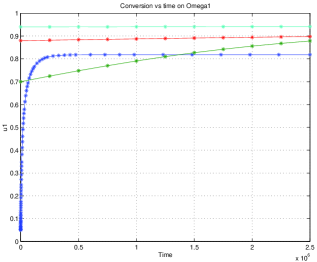
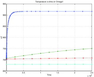
Figure 2: Simulations of the conversion and temperature for three initials conditions in $\Omega_{1}$

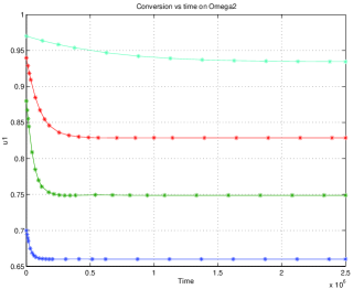
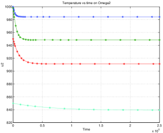
Figure 3: Simulations of the conversion and temperature for three initials conditions in $\Omega_{2}$

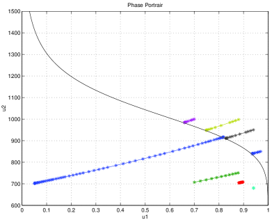
Figure 4: Phase portrait

The numerical evidences suggest that there exists sufficient conditions to state that all $\mathbf{u}=\mathbf{u}(t)$ of the system with initial value $\mathbf{u}^{0}=\mathbf{u}(0)\in\Omega_{i}$, $i=1$ or $i=2$, be it sufficiently close or distant to a steady-state $\mathbf{u}^{e}\in\Gamma$, remain confined on $\Omega_{i}$, for $i=1$ or $i=2$, and tend to this steady-state when time $t$ tends to infinite. Then if $\mathbf{u}^{0}=\mathbf{u}(0)\in\Omega_{1}$ and $\mathbf{\mathbf{u}}(t)\rightarrow\mathbf{u}^{e}$ when $t\rightarrow\infty$ we can assume that on $\Omega_{1}$ each component $u_{i}(t)$, for $i=1,2$, is an monotone increasing function or in fact that for any $\mathbf{u}(t)\in\Omega$ the vectorial field $\mathbf{u}^{\prime}(t)=\mathbf{f}(\mathbf{u}(t))$ has strictly positive sign. Similarly, if $\mathbf{u}^{0}=\mathbf{u}(0)\in\Omega_{2}$ and $\mathbf{\mathbf{u}}(t)\rightarrow\mathbf{u}^{e}$ when $t\rightarrow\infty$ on $\Omega_{2}$ each component $u_{i}(t)$, for $i=1,2$, is an monotone decreasing function or in fact that for any $\mathbf{u}(t)\in\Omega$ the vectorial field $\mathbf{u}^{\prime}(t)=\mathbf{f}(\mathbf{u}(t))$ has strictly negative sign. In order to establish these affirmations formally, we have the following results.

Proposition 4.

Let $(\xi_{1},\xi_{2})$ be a point in $\Omega_{1}$ where a solution of problem (LABEL:eq9.1) begins. The vectorial field $\mathbf{u}^{\prime}(t)=\mathbf{f}(\mathbf{u}(t))$ is strictly positive on $\Omega_{1}$ for all time $t$ in the interval $I(\xi_{1},\xi_{2})\cap[0,\infty)$.

Proof. Let $(\xi_{1},\xi_{2})\in\Omega_{1}$ be the corresponding point to the initial condition for problem (LABEL:eq9.1) in $t_{0}=0$, such that $\mathbf{u}^{\prime}(0)=\mathbf{f}(\xi_{1},\xi_{2})=\left(f_{1}(\xi_{1},\xi_{2}),f_{2}(\xi_{1},\xi_{2}))\right)$. Then the sign of vectorial field $\mathbf{f}$ on $\Omega_{1}$ depends on the sign that takes each component $f_{i}$, $i=1,2$ for all initial point $(\xi_{1},\xi_{2})\in\Omega_{1}$ and all $t\in I(\xi_{1},\xi_{2})\cap[0,\infty)$. Indeed

$$f_{1}(\xi_{1},\xi_{2})=\beta_{1}g_{1}(\xi_{1})K_{1}(\xi_{2})K_{2}(\xi_{1})K_{3}(\xi_{1},\xi_{2})\hskip 8.5359pt\mbox{and}\hskip 8.5359ptf_{2}=f_{1}(\xi_{1},\xi_{2})g_{2}(\xi_{1},\xi_{2}),$$

where if the constant $\beta_{1}$ is positive and by definition, for all points of the domain, $\Omega$, functions $g_{1}$, $K_{1}$, $K_{2}$ and $g_{2}$ are strictly positive, then the sign of $f_{1}(\xi_{1},\xi_{2})$ and $f_{2}(\xi_{1},\xi_{2})$ will be positive only if $K_{3}(\xi_{1},\xi_{2})$ has strictly positive sign. This can be verified if we assume that there exists a point $(\xi_{1},\xi_{2})\in\Omega_{1}$ for which $K_{3}(\xi_{1},\xi_{2})\leq 0$. Then if $K_{3}(\xi_{1},\xi_{2})=0$ implies that $\xi_{2}=u_{2}^{e}$, which is a contradiction because by definition of subset $\Omega_{1}$ must satisfy that $\xi_{2}<u_{2}^{e}$. Similarly, if $K_{3}(\xi_{1},\xi_{2})<0$ then, fixing $\xi_{1}\in(0,u_{1}^{\ast})$, we find that $\frac{1}{u_{2}^{e}}>\frac{1}{\xi_{2}}$ implying that $\xi_{2}>u_{2}^{e}$; again a contradiction. With this we verified that $K_{3}(\xi_{1},\xi_{2})>0$ for all $(\xi_{1},\xi_{2})\in\Omega_{1}$ and we concluded the proof. $\blacksquare$

The next proposition is proved in a similar way.

Proposition 5.

Let $(\zeta_{1},\zeta_{2})$ be a point in $\Omega_{2}$ where a solution of problem (LABEL:eq9.1) begins. The vectorial field $\mathbf{u}^{\prime}(t)=\mathbf{f}(\mathbf{u}(t))$ is strictly negative on $\Omega_{2}$ for all time $t$ in the interval $I(\zeta_{1},\zeta_{2})\cap[0,\infty)$.

Based on the two previous propositions, with the following corollary we establish the important property on the behavior of the solutions in $\Omega_{1}$ and $\Omega_{2}$ that was demonstrated in the numerical simulations.

Corollary 2.

For each $i=1,2$, solutions $u_{i}(t)$ of the problem (LABEL:eq9.1) are increasing functions on $\Omega_{1}$ and decreasing functions on $\Omega_{2}$ for all $t\geq t_{0}$.

Finally, the confinement property of the solutions in each $\Omega_{i}$, $i=1,2$, and the tendency of these to a stationary point of $\Gamma$ when time $t$ tends to infinite is established with the following lemma.

Lemma 1.

All solution $\mathbf{u}(t)$ of (LABEL:eq9.1) that begins in the region defined by subdomain $\Omega_{i}$, for each $i=1,2$, in the time $t=t_{0}$ remains in that region for all future time $t\geq t_{0}$, and finally tends to the stationary solution in $\Gamma$.

Proof. The proof shall be presented schematically for $\Omega_{1}$; for $\Omega_{2}$ is similar.

We assume that a solution $\mathbf{u}(t)=\left(u_{1}(t),u_{2}(t)\right)$ of (LABEL:eq9.1) leaves the region defined by $\Omega_{1}$ in time $t=t^{\ast}$. Then $\mathbf{u}^{\prime}(t^{\ast})=\mathbf{0}$, since the unique way in which a solution can leave the region defined by $\Omega_{1}$ is crossing curve $\Gamma$.

Corollary 2 assures this, because it indicates that in that region $\mathbf{u}^{\prime}(t)>0$ for all $t$. On the other hand the study of existence and uniqueness of solution of the problem (LABEL:eq9.1) guarantees that two solutions cannot be cut. For such reason, as $\Gamma$ is the set of trivial solutions of the problem, any solution that begins in $\Omega_{1}$ will not cross a solution in $\Gamma$. Then, this contradicts the fact that $\mathbf{u}^{\prime}(t^{\ast})=\mathbf{0}$, assuring that the solutions initiated in $\Omega_{1}$ remain in that region for all future time $t\geq t_{0}$. In addition, this implies that each $u_{i}(t)$, $i=1,2$, is an monotone increasing function of the time for $t\geq t_{0}$ that is bounded in such region, therefore has a limit when $t$ tends to infinite. We only must verify that this limit is a component of all point in $\Gamma$. Indeed, if we denote $\eta_{i}$ the limit of each function $u_{i}(t)$ when $t$ tends to infinite, then this will imply that $\left|u_{i}(t_{1})-u_{i}(t_{2})\right|$ tends to zero when $t_{1}$ and $t_{2}$ tend to infinite, since

$$\left|u_{i}(t_{1})-u_{i}(t_{2})\right| = \left|\left(u_{i}\left(t_{1}\right)-\eta_{i}\right)+\left(\eta_{i}-u_{i}\left(t_{2}\right)\right)\right|$$

$$\leq \left|u_{i}\left(t_{1}\right)-\eta_{i}\right|+\left|u_{i}\left(t_{2}\right)-\eta_{i}\right|.$$

In particular, let $t_{1}=t$ and $t_{2}=t_{1}+\kappa$ for some fixed positive number $\kappa$. Then, $\left|u_{i}(t+\kappa)-u_{i}(t)\right|$ tends to zero when $t$ tends to infinite. But

$$u_{i}(t+\kappa)-u_{i}(t)=\kappa\frac{du_{i}(\tau)}{dt}=\kappa f_{i}\left(u_{1}(\tau),u_{2}(\tau)\right)$$

where $\tau$ is an arbitrary number between $t$ and $t+\kappa$. We observe finally that $f_{i}\left(u_{1}(\tau),u_{2}(\tau)\right)$ must tend to $f_{i}\left(\eta_{1},\eta_{2}\right)$ when $t$ tends to infinite. Therefore, $f_{i}\left(\eta_{1},\eta_{2}\right)=0$ for each $i=1,2$, and with this we conclude the proof. $\blacksquare$

Lemma 1 guarantees that solutions of the system that begin either in subdomains, $\Omega_{1}$ and $\Omega_{2}$, tend to a steady-state located on curve $\Gamma$ when the time tends to infinite whatever the initial starting condition within each region is, therefore situation shown in the figure 5, and illustrated on each subdomain for the curves drawn up by segments that start in $(\xi_{1}^{0},\xi_{2}^{0})\in\Omega_{1}$ and in $(\zeta_{1}^{0},\zeta_{2}^{0})\in\Omega_{2}$, cannot happen.

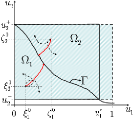
Figure 5: Situations that cannot happen with $\mathbf{u}(t)$

V Brief discussion

The two regions $\Omega_{1}$ and $\Omega_{2}$ characterized in this work, are the regions in which both direct and inverse chemical reaction take place. This can be affirmed because we demonstrated with Corollary (2) that in $\Omega_{1}$ when increasing the conversion of $\mbox{SO}_{2}$, the temperature of the system increases too; indeed, $\Omega_{1}$ is the region where the exothermic character of the reaction predominates. Similarly, it is proved that the region defined by $\Omega_{2}$ is where the endothermic character of the reaction predominates (diminution of the conversion of $\mbox{SO}_{2}$ and temperature of the system).

On the other hand, with Lemma 1 we demonstrated that the solutions of the model (LABEL:eq9.1) tend to a steady-state whatever the starting state in $\Omega_{i}$, for each $i=1,2$, and remain confined in this region. This behavior is consistent with the physical phenomenon, since, experimentally we know that with very long time steps the reaction tends to the equilibrium because always there exist infinitesimal changes in the conversion and temperature; which define states called quasi-steady states.

Also we know that the course of reaction changes if the system is perturbed providing or removing energy from it. This perturbation will locate the reaction in a new initial state on the same subdomain or on the other subdomain; in the latter, the change of subdomain is not a natural behavior of the system. This change is caused by an external factor that modifies the initial conditions of the problem; therefore, the solutions of the mathematical model must remain in the origin region as long as they are not perturbed.

VI Conclusions

The solutions of a mathematical model that is used to analyze the dynamic behavior of reversible reaction $\mbox{SO}_{2\,(\mathrm{g})}\,+\,\frac{1}{2}\,\mbox{O}_{2\,(\mathrm{g})}\,\rightleftharpoons\,\mbox{SO}_{3\,(\mathrm{g})}$ carried out in a catalytic reactor, were studied qualitatively by means of the abstraction of the model in terms of the state variables: conversion of the $\mbox{SO}_{2}$ and temperature of the system. In this sense, we demonstrated that the model is a well-posed Cauchy problem; i.e., there exists an unique solution for each initial condition related to the state variables.

The trivial solutions of the mathematical model correspond with the steady-states of the reactive system and conform a continuous front on the phase portrait for conversion versus temperature. In fact, the phase portrait was divided in two separated regions by the continuous steady-states, and we demonstrated that in a region the reaction advances exothermically and in the other region it advances endothermically as we expect from the physicochemical point of view. Also, we proved that when time becomes sufficiently large, conversion of the $\mbox{SO}_{2}$ and temperature of the reactive system will remain near some steady-state whatever the point in the phase portrait from which the state variables begin. All these theoretical results were complemented with numerical simulations by means of which we observed a priori the hypotheses and conclusions of the Propositions, Corollaries and Lemmas that we presented in this article.

References

- (1) Amann H. , Ordinary Differential Equations: An Introduction to Nolinear Analysis. De Gruyter. Walter, 1990.
- (2) Angulo W., Contreras J., Crespo M., Toro J. y Verrushi M., Simulación Dinámica de una Reacción Catalítica, Tesis de la Universidad Experimental Politécnica Antonio José de Sucre, Barquisimeto-Venezuela, 2003.
- (3) Bartle R.G., Introducción al Análisis Matemático, Limusa Noriega, México, España, Venezuela, 1990.
- (4) Bales V., Acai P., Mathematical analysis of the performance of a packed bioreactor with immobilised cells., Recents Progress en Genierdes Procedes, 13, 71, (1999), 335–342.
- (5) Carberry, J. Chemical and Catalytic Reaction Engineering, Mc Graw Hill, USA, 1976.
- (6) Carberry J.J., Wendel M.M., Computer model of the fixed catalytic reactor., A.I.Ch.E. Journal, 9, (1963), 129–133.
- (7) Coddington E. and Levinson N., Theory of Ordinary Differential Equations. McGraw-Hill, New York, 1995.
- (8) Fogler, S. Elementos de Ingeniería de las Reacciones Químicas, Editorial Prentice Hall, 3ra edition, 2001.
- (9) Irribarren I., Cálculo Diferencial en Espacios Normados, EQUINOCCIO, Ediciones de la Universidad Simón Bolívar (USB), Caracas-Venezuela, 1980.
- (10) Mars, P. and Maessen, J. The Mechanism and the Kinetics of Sulfur Dioxide Oxidation on Catalyst Containing Vanadium an Alcali Oxide, Journal of Catalisis, 10 (1968), 51–55.
- (11) Parzynski W.R. and Zipse P.W., Introduction to Mathematical Analysis, McGraww-Hill, New York, St. Louis, 1982.
- (12) Tineo A. y Rivero J., Ecuaciones Diferenciales Ordinarias, Publicación de la Universidad de los Andes, Mérida-Venezuela, 2002.