Generalized Uncertainty Principle Corrections to the Simple Harmonic Oscillator in Phase Space

Abstract

We compute Wigner functions for the harmonic oscillator including corrections from generalized uncertainty principles (GUPs), and study the corresponding marginal probability densities and other properties. We show that the GUP corrections to the Wigner functions can be significant, and comment on their potential measurability in the laboratory.

, ,

Keywords: generalized uncertainty principle, harmonic oscillator, Wigner functions, phase space quantum mechanics, quantum gravity

1 Introduction

It is currently not possible to access the natural energy scale of quantum gravity, the Planck energy. It is feasible, however to consider low-energy effects, e.g., the quantum-gravity induced perturbative corrections to non-relativistic quantum mechanics. One avenue is the study of corrections to the Schrödinger equation originating from the GUP proposed in various candidate theories of quantum gravity (such as string theory, loop quantum gravity, etc.). A modification is postulated of the usual Heisenberg algebra (and the resulting Heisenberg uncertainty principle), to

$$[\hat{x}_{i},\hat{p}_{j}]\ =\ i\hbar\,f_{i,j}(\hat{p})\ .$$ (1)

For the 1-dimensional case considered in this paper, $f_{i,j}$ becomes a single function, $f(p)$. In [1], the quadratic form $f(p)=1+\beta p^{2}$ was suggested, while in [2], a linear $+$ quadratic function,

$$f(p)\ =\ 1\,+\,\alpha p\,+\,\beta p^{2}\,,\ \$$ (2)

was proposed. Here $\alpha=\alpha_{0}/{M_{\rm Pl}\,c}=\alpha_{0}\ell_{\rm Pl}/\hbar,M_{\rm Pl}=$ Planck mass, $\ell_{\rm Pl}\approx 10^{-35}~{}$metre = Planck length. $\alpha_{0}$ can be assumed to be order unity, and $\beta={\cal O}(\alpha^{2})$.

Over the years, various modifications of the canonical commutation relations have been considered, with many different motivations. We focus on (1, 2) because we are ultimately interested in the low-energy effects of quantum gravity, and because, in that context, modifications (1, 2) are quite general. The form (2) of $f(p)$ has been suggested by various approaches to quantum gravity, as well as from black hole physics and doubly special relativity theories [5]. Various perturbative and non-perturbative effects of the correction terms were studied in a number of papers including those for low energy systems, the fundamental nature of spacetime, and cosmology (for a related review, see [6]; see also references therein).

Naturally, one of the first examples studied in this context was the harmonic oscillator, in which GUP corrections to the eigenvalues and eigenfunctions were computed [1, 2]. It is anticipated that effects of at least some of these corrections may be observable in the low energy laboratory, for example in quantum optics.

To explore this further, in this paper we study the GUP corrections to the harmonic oscillator in phase space, and in particular compute and plot the Wigner functions corresponding to the unperturbed and perturbed eigenfunctions for various $n$, and then study their differences. We note that, depending on the value of $\alpha_{0}$, these differences could be significant, and therefore in principle may have observational consequences. In the following sections, we briefly review Wigner functions, and compute and plot them for the problem described above. In the concluding section, we comment on potential applications.

2 Wigner Functions

Rather than using the operator formalism, it is possible to work with a phase-space formulation of quantum mechanics, developed by Groenewold and Moyal. In it, observables are represented by (generalized) functions in phase space, that are multiplied using an associative (Moyal) star product,

$$\star\ =\ \exp\left\{\frac{i\hbar}{2}\left(\overleftarrow{\partial_{x}}\,\overrightarrow{\partial_{p}}-\overleftarrow{\partial_{p}}\,\overrightarrow{\partial_{x}}\right)\right\}\ ,$$ (3)

and states are described by the well-known Wigner function (see [8], e.g., for recent reviews, and [9] for pedagogical treatments). The Wigner transform maps an operator $\hat{g}$ to the corresponding phase-space function,

$${\cal{W}}(\hat{g})=\hbar\int dy\,e^{-ipy}\left\langle x+{\hbar y}/{2}\big{|}\,\hat{g}\,\big{|}x-{\hbar y}/{2}\right\rangle\ ,$$ (4)

such that the star product of observables in phase space is homomorphic to the operator product,

$${\cal W}\big{(}\hat{a}\,\hat{b}\big{)}\ =\ {\cal W}(\hat{a})\,\star\,{\cal W}(\hat{b})\ .$$ (5)

Up to a multiplicative constant, the Wigner function is nothing but the Wigner transform of the density matrix $\hat{\rho}$:

$$W(x,p)\,=\,\frac{{\cal{W}}(\hat{\rho})}{2\pi\hbar}\,=\,\frac{{\cal{W}}(\ket{\psi}\bra{\psi})}{2\pi\hbar}\,=\,\frac{1}{2\pi}\int_{-\infty}^{\infty}\,\psi^{*}\left(x-{\hbar y}/{2}\right)\,\psi\left(x+{\hbar y}/{2}\right)\,e^{-ipy}\,dy\ .$$ (6)

Here $\hat{\rho}$ is the density matrix, $\psi$ is the wave function in $x$-space, $x$ is the position, and $p$ is the momentum. The Wigner function can also be found using the wave function, $\phi$, in $p$-space:

$$W(x,p)=\frac{1}{\hbar}\int_{-\infty}^{\infty}\phi^{*}\left(p+{u}/{2}\right)\,\phi\left(p-{u}/{2}\right)\,e^{ixu/\hbar}\,du\ .$$ (7)

One other alternative method to find the Wigner function is to solve the stargenvalue equations

$$H\star W(x,p) \ =\ E\,W(x,p)\ ,$$ (8)

$$W(x,p)\star H \ =\ E\,W(x,p)\ \ .$$ (9)

$H$ is the Hamiltonian of the system, and $E$ is the energy.
For example, Figure 1 displays the Wigner functions of two energy eigenstates of the simple harmonic oscillator.
Important properties of the Wigner function include: (i) reality, $W(x,p)=W(x,p)^{*}$, (ii) position probability density, $P(x)=|\psi(x)|^{2}=\int W(x,p)\,dp$, (iii) momentum probability density, $P(p)=|\phi(p)|^{2}=\int W(x,p)\,dx$, and (iv) normalization, $\int W(x,p)\,dx\,dp=1$. Using the Wigner function, the expectation value $\langle a\rangle$ of an operator $\hat{a}$ is

$$\langle a\rangle\ =\ \int\,W(x,p)\,a(x,p)\,\,dx\,dp\ ,$$ (10)

where $a(x,p)={\cal W}(\hat{a})$ is the Weyl transform of $\hat{a}$.

The equivalence of phase space quantum mechanics to the operator formulation follows from the Wigner transform ${\cal W}$, and its inverse, ${\cal W}^{-1}$, known as the Weyl map. The latter’s relation to Weyl operator ordering is made plain by expanding

$${\cal W}^{-1}\left(e^{\zeta x+\eta p}\right)\ =\ e^{\zeta\hat{x}+\eta\hat{p}}\$$ (11)

in powers of $\zeta$ and $\eta$. This last equation also indicates how general functions in phase space map to operators: Fourier component by component.

Using $[\hat{x},\hat{p}]=i\hbar$ and a simple Baker-Campbell-Hausdorff formula, one finds

$$\exp\left(\zeta\hat{x}+\eta\hat{p}\right)\,\exp\left(\zeta^{\prime}\hat{x}+\eta^{\prime}\hat{p}\right)\ =\ \exp\left[(\zeta+\zeta^{\prime})\hat{x}+(\eta+\eta^{\prime})\hat{p}\right]\,\exp\left[i\hbar(\zeta\eta^{\prime}-\eta\zeta^{\prime})/2\right]\ ,$$ (12)

the defining relation of the Heisenberg-Weyl group. Then (5) leads to the form (3) of the Moyal star product.

If the Heisenberg commutation relations are generalized to $[\hat{x},\hat{p}]=i\hbar(1+\alpha\hat{p}+\beta\hat{p}^{2})$, then a similar computation yields a modified GUP star product

$$\log\left(\,\tilde{\star}\,\right)\ =\ \log\left(\,\star\,\right)\,\cdot\,\left\{\,F_{0}\,+\,\frac{F_{1}}{6}\,\left(\overleftarrow{\partial_{x}}-\overrightarrow{\partial_{x}}\right)\,-\,\frac{F_{2}}{12}\,\overleftarrow{\partial_{x}}\,\overrightarrow{\partial_{x}}\,+\,\ldots\,\right\}\ .$$ (13)

Here

$$F_{n}\ :=\ \left[i\hbar f(p)\frac{d}{dp}\right]^{n}\,f(p)\ ,$$ (14)

and the exponent in (13) does not terminate for polynomial $f(p)$, such as (2). This GUP star product encodes completely the effects of the GUP in phase-space quantum mechanics. As a simple example, the $\tilde{\star}$-commutator realizes the generalized commutation relation $x\tilde{\star}p-p\tilde{\star}x=i\hbar f(p)$.

Clearly, it is impracticable to solve equations (8)-(9) for the GUP-corrected Wigner functions, if the GUP star product $\tilde{\star}$ is used. We will instead take the simpler approach of finding the GUP-corrected wave functions in momentum space first (building on the work of [1]), and then use (7) to calculate the Wigner functions.

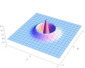
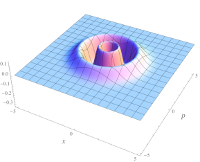
Figure 1: The simple harmonic oscillator Wigner functions for $n=2$ (left) and $n=3$ (right). With $m=\hbar=\omega=1$, they only depend on $x^{2}+p^{2}$; the circular symmetry is evident. Because the Wigner function can be negative, it is known as a quasi-probability distribution.

3 Corrections to harmonic oscillator from quadratic GUP

We will first review the work of [1] in which $f(p)=1+\beta p^{2}$, the simplest case of the previously mentioned quantum gravity phenomenologies ($\alpha=0$), for which the GUP assumes the form

$$\Delta x\Delta p\geq\frac{\hbar}{2}\left(1+\beta\langle{p^{2}}\rangle\right)\,\ .$$ (15)

For small $\beta$, with $\displaystyle{\epsilon=2E/m\hbar^{2}\omega^{2}}$ and $\displaystyle{\eta^{2}=1/(m\hbar\omega)^{2}}$ , the GUP-corrected Schrödinger equation for the harmonic oscillator in momentum space becomes [1]

$$\frac{d^{2}\phi(p)}{dp^{2}}+\frac{2\beta p}{1+\beta p^{2}}\frac{d\phi(p)}{dp}+\frac{1}{\left(1+\beta p^{2}\right)^{2}}\left[\epsilon-\eta^{2}p^{2}\right]\phi(p)=0\,.$$ (16)

The solution is [1]

$$\phi(p)\,=\,\frac{{\cal N}}{\left(1+\beta p^{2}\right)^{\sqrt{q+r}}}\ {}_{2}F_{1}\left(a,b;c;\frac{1}{2}+i\frac{\sqrt{\beta}}{2}p\right)\,,$$ (17)

where $q=\epsilon/4\beta,\ r=\eta^{2}/4\beta^{2},\ a=\frac{1}{2}\left(1-\sqrt{1+16r}\right)-2\sqrt{q+r},\ b=\frac{1}{2}\left(1+\sqrt{1+16r}\right)-2\sqrt{q+r},\ c=1-2\sqrt{q+r}.$ The solution is normalizable, with normalization constant ${\cal N}$, if $b=-n\in{\mathbb{Z}}^{-}\cup\{0\}$ ($a$, $c$, and $\sqrt{q+r}$ can each be expressed in terms of $n$). The energy eigenvalues are then [1]

$$E_{n}=\hbar\omega\left(n+\frac{1}{2}\right)\left(\frac{\beta}{2\eta}+\sqrt{1+\frac{\beta^{2}}{4\eta^{2}}}\right)+\hbar\omega\frac{\beta}{2\eta}n^{2}\ .$$ (18)

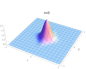
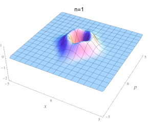
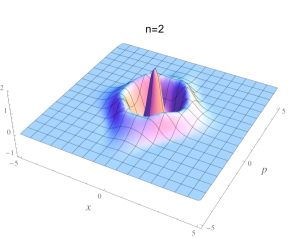
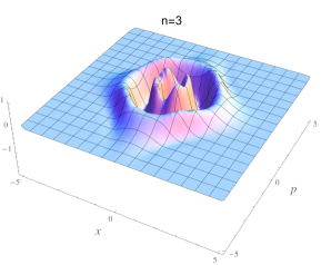
Figure 2: $n=0,1,2,3$ Wigner functions of the simple harmonic oscillator with a GUP correction for vanishing $\alpha$ ( see equation (2) ). We have set $m=\epsilon=\eta=1$ and $\beta=0.1$. Notice that the circular symmetry is broken, but the quasi-probability distributions are unchanged by $p\to-p$, and/or $x\to-x$.

The normalization constant in (17) is

$${\cal N}=\bigg{(}2^{\,k+m}\sqrt{\beta}\sum_{k,m=0}^{n}\lambda_{km}\tau_{km}\bigg{)}^{-1/2}\,,$$ (19)

where

$$\lambda_{km}=\frac{(a)_{k}(a)_{m}(-n)_{k}(-n)_{m}}{(c)_{k}(c)_{m}k!m!}$$ (20)

(given in terms of the Pochhammer symbol) and

$$\tau_{km}=\frac{i}{\mu}\big{[}\pi A(\mu,\kappa)-B(\mu,\kappa)\big{]}+\frac{i}{\kappa}\big{[}\pi A(\kappa,\mu)-B(\kappa,\mu)\big{]}\,,$$ (21)

with

$$\kappa=k-2\sqrt{q+r}+1\,,$$

$$\mu=m-2\sqrt{q+r}+1\,,$$

$$A(\mu,\kappa)=\frac{2^{\kappa+\mu-1}\Gamma(\mu+1)e^{i\pi\mu}\csc(\kappa+\mu)}{\Gamma(1-\kappa)\Gamma(\kappa+\mu)}\,,$$

$$B(\mu,\kappa)=2^{\kappa+\mu-1}\,{}_{2}F_{1}(\kappa+\mu,\kappa;\kappa+1;-1).$$ (22)

So far, we have reviewed the results obtained by [1]. As a new contribution, we will now consider the Wigner functions for the wave functions just described. By numerically integrating equation (7), using equation (17), we found the Wigner functions associated with the simple harmonic oscillator corrected by a GUP motivated by quantum gravity (Figure 2).

Notice the deformation of the circular symmetry about the centre of the Wigner function. The quasi-probability distributions remain invariant under parity tranformations in both $x$- and $p$-space, however. See also the probability densities plotted in Figure 3. Unlike for the regular simple harmonic oscillator, which enjoys symmetry under $x\leftrightarrow-p$, the two probability densities do not look the same.

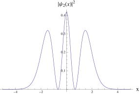
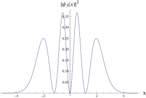
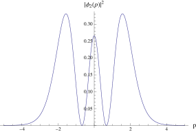
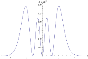
Figure 3: The probability densities of the GUP-corrected $n=2$ and $n=3$ simple harmonic oscillator energy eigenstates for $\alpha=0,\beta\not=0$. The top two plots are the $x$-space densities while the bottom plots are in $p$-space. The transformations $x\to-x$ and $p\to-p$ leave the densities invariant. We have set $m=\omega=\hbar=1$ and $\beta=0.1$.

4 Corrections to harmonic oscillator from linear + quadratic GUP

Next, we consider the modified Heisenberg algebra proposed in [2], corresponding to the quantum gravity phenomenology described by (2) in (1). The GUP is now

$$\Delta x\Delta p\ \geq\ \frac{\hbar}{2}\left(1+\alpha\langle p\rangle+\beta\langle p^{2}\rangle\right)\ ,$$ (23)

and the time-independent Schrödinger equation is

$$\frac{d^{2}\phi(p)}{dp^{2}}+\frac{\alpha+2\beta p}{1+\alpha p+\beta p^{2}}\,\frac{d\phi(p)}{dp}+\frac{\epsilon-\eta^{2}p^{2}}{\left(1+\alpha p+\beta p^{2}\right)^{2}}\,\phi(p)\,=\,0\,,$$ (24)

with $\epsilon$ and $\eta$ as defined above. Letting

$$\phi(p)\,=:\,\Phi(z)\,,\quad\ z\,=\,\frac{{2\beta p+\alpha+\sqrt{\alpha^{2}-4\beta}}}{2{\sqrt{\alpha^{2}-4\beta}}}\ ,$$ (25)

we can convert equation (24) into the form of the Riemann equation:

$$\frac{d^{2}\Phi(z)}{dz^{2}}\,+\,\frac{(2z-1)}{z\left(z-1\right)}\frac{d\Phi(z)}{dz}\,+\,\frac{q-r\left(\alpha+\sqrt{\alpha^{2}-4\beta}-2z\sqrt{\alpha^{2}-4\beta}\right)^{2}}{z^{2}\left(z-1\right)^{2}}\Phi(z)\,=0\ ,$$ (26)

where

$$q=\frac{\epsilon}{\left(\alpha^{2}-4\beta\right)}\,,\hskip 28.45274ptr=\frac{\eta^{2}}{4\beta^{2}\left(\alpha^{2}-4\beta\right)}\ .$$ (27)

Solving using the Riemann $P$-symbol [10],

$$\Phi(z)\propto\mathcal{P}\left\{\begin{array}[]{cccc}0&1&\infty\\ s&t&u_{-}&z\\ -s&-t&u_{+}\end{array}\right\}=z^{s}(1-z)^{t}\,{}_{2}F_{1}\left(a,b;c;z\right)\ ,$$ (31)

where

$$s=-\sqrt{-q+2r\alpha^{2}+2r\alpha\sqrt{\alpha^{2}-4\beta}-4r\beta}\ ,$$

$$t=-\sqrt{-q+2r\alpha^{2}-2r\alpha\sqrt{\alpha^{2}-4\beta}-4r\beta}\ ,$$

$$u_{\pm}=\frac{1}{2}\left(1\pm\sqrt{1+\frac{4\eta^{2}}{\beta^{2}}}\right)\ ,$$

$$a=u_{-}+s+t\,,\hskip 28.45274ptb=u_{+}+s+t\,,\quad c=1+2s\ .$$ (32)

With no restrictions on $\alpha$ and $\beta$, we note that there exist non-integrable singularities. However, if we assume $\alpha^{2}<4\beta$, we find $s=t^{*}$, thus, eliminating this problem.

To analyze the asymptotics of the wave function, we use $z^{v}w^{v^{*}}=z^{x+iy}w^{x-iy}=(zw)^{x}e^{iy\ln\left(\frac{z}{w}\right)},$ valid for arbitrary $z,v,w\in{\mathbb{C}},$ $x,y\in{\mathbb{R}}$. We find

$$\Phi(z)\propto\left[z(1-z)\right]^{{\rm Re}(s)}e^{i\,{\rm Im}(s)\ln\frac{z}{1-z}}\,{}_{2}F_{1}\left(a,b;c;z\right)\ .$$ (33)

Since we want to ensure that the square of the norm of the wave function converges when integrated, we consider two cases: 1) $a=-n$ and 2) $b=-n$; here $n\in{\mathbb{Z}}^{+}\cup\{0\}$ so that the Gauss hypergeometric function reduces to a polynomial of order $n$. For $a=-n$, we find:

$$b=-n+\sqrt{1+\frac{4\eta^{2}}{\beta^{2}}}\,,$$

$$c=1-n-u_{-}+2i\,{{\rm Im}}(s),$$

$${{\rm Re}}(s)=-\frac{n+u_{-}}{2}\,,$$ (34)

so that

$$\Phi_{1}(z)\ =\ \left[z(1-z)\right]^{-\frac{n+u_{-}}{2}}e^{i\,{{\rm Im}}(s)\,\ln\frac{z}{1-z}}\,{}_{2}F_{1}\left(-n,-n+\sqrt{1+\frac{4\eta^{2}}{\beta^{2}}};1-n-u_{-}+2i\,{{\rm Im}}(s);z\right)$$

$$\sim z^{-u_{-}}\ ,\ \ {\rm for\ large}\ |z|\ \ .$$ (35)

For $b=-n$:

$$a=-n-\sqrt{1+\frac{4\eta^{2}}{\beta^{2}}}\,,$$

$$c=1-n-u_{+}+2i\,{{\rm Im}}(s)\,,$$

$${{\rm Re}}(s)=-\frac{n+u_{+}}{2}\,,$$ (36)

so that

$$\Phi_{2}(z)\ =\ \left[z(1-z)\right]^{-\frac{n+u_{+}}{2}}\,e^{i\,{{\rm Im}}(s)\ln\frac{z}{1-z}}\,{}_{2}F_{1}\left(-n-\sqrt{1+\frac{4\eta^{2}}{\beta^{2}}},-n;1-n-u_{+}+2i\,{{\rm Im}}(s);z\right)$$

$$\sim z^{-u_{+}}\ ,\ \ {\rm for\ large}\ |z|\ \ .$$ (37)

We see that, as $z\to\infty$, $\Phi_{1}$ diverges, thus $\phi(p)\propto\Phi_{2}(z)$,

$$\phi(p)\,\propto\,\left[\alpha^{2}-4\beta-(2p\beta+\alpha)^{2}\right]^{-\frac{n+u_{+}}{2}}\exp\left\{i\,{{\rm Im}}(s)\,\ln\left[\frac{2\,p\beta+\alpha+\sqrt{{\alpha}^{2}-4\,\beta}}{\sqrt{{\alpha}^{2}-4\,\beta}-2\,p\beta-\alpha}\right]\right\}$$

$${}\quad\times\,{}_{2}F_{1}\left(-n-\sqrt{1+\frac{4\eta^{2}}{\beta^{2}}},-n;1-n-u_{+}+2\,{{\rm Im}}(s);\,\frac{2\beta p+\alpha+\sqrt{\alpha^{2}-4\beta}}{2\sqrt{\alpha^{2}-4\beta}}\right)\ .$$ (38)

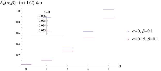
Figure 4: Energy levels are indicated for the simple harmonic oscillator with the 1-parameter GUP correction (blue, $\alpha=0$, $\beta=0.1$), and with the 2-parameter GUP correction (red, $\alpha=0.15$, $\beta=0.1$). The differences between the corrected and uncorrected energies are shown; in all cases they are larger for the 1-parameter correction. The inset shows the small energy difference between the 2 cases for $n=0$. We have set $m=\epsilon=\eta=\hbar=1$.

4.1 GUP Corrected Energy Spectrum

Using

$$\epsilon=\frac{2E}{\hbar^{2}\omega^{2}}\ ,\qquad q=\frac{\epsilon}{(\alpha^{2}-4\beta)}\ ,\qquad-n=b=u_{+}+s+t\ ,$$ (39)

we find that

$$E_{n} \ =\ \frac{\alpha^{2}m\omega^{2}\hbar^{2}\left[n\xi\left(2\sigma\left\{1+\theta+n[3\xi+2\theta]\right\}-n\xi\sigma^{2}\left\{1+\theta+2n[\xi+\theta]\right\}-8\right)-2\right]}{16\left(\sigma n^{2}+\sigma n-1\right)^{2}}$$ (40)

$$\qquad\qquad\qquad+\ \frac{4\beta m\omega^{2}\hbar^{2}\left[1+\theta+2n(\xi+\theta)\right]\left[n\xi\sigma-1\right]^{2}}{16(\sigma n^{2}+\sigma n-1)^{2}}\ ,$$

where $\displaystyle{\theta=\sqrt{1+\frac{4}{\sigma}}}$, $\xi=1+n$, and $\sigma=(m\beta\omega\hbar)^{2}$. Note that for $\alpha\to 0$, the spectrum (18) is recovered. Subsequently taking $\beta\to 0$, the energies reduce to the expected $E_{n}=\left(n+1/2\right)\hbar\omega$.

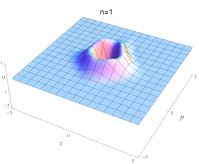
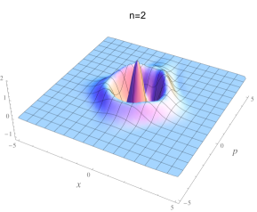
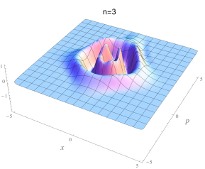
Figure 5: GUP-corrected Wigner functions with $\alpha=0.15$ and $\beta=0.1$. We have set $m=\epsilon=\eta=\hbar=1$.

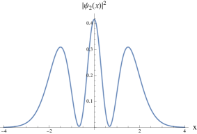
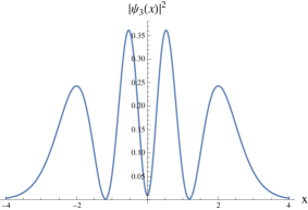
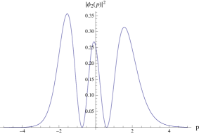
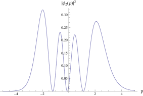
Figure 6: GUP-corrected probability densities with $\alpha=0.15$ and $\beta=0.1$ for $n=2$ and $n=3$. The top (bottom) 2 plots show $x$-space ($p$-space). The symmetry $x\to-x$ ($p\to-p$) is intact (broken). We have set $m=\epsilon=\eta=\hbar=1$.

Figure 4 depicts the lowest energies ($n=0,\ldots,4$) of the spectra for $\alpha=\beta=0$ (unperturbed simple harmonic oscillator), $\alpha=0$, $\beta=0.1$ (simple harmonic oscillator with 1-parameter GUP correction), and $\alpha=0.15$, $\beta=0.1$ (simple harmonic oscillator with 2-parameter GUP correction). Notice that, even for small $n$, the difference in energy levels grows rapidly. Also, while the perturbations raise the energies in both cases, the effect is smaller when both $\alpha,\beta\not=0$.

4.2 GUP Corrected Wigner Functions

The quantum gravity-modified Wigner functions for a GUP (2) with both $\alpha$ and $\beta$ non-vanishing (Figure 5) exhibit a modified deformation from that for $\alpha=0$ (Figure 2), with the difference becoming clearer as $n$ becomes larger. While invariance under $x\to-x$ remains intact, symmetry under $p\to-p$ is broken.

Correspondingly, the probability densities for the 2-parameter GUP correction differ from those for the 1-parameter case (Figure 6). Note that the disappearance of the symmetry between the $x$- and $p$-space probability densities is more pronounced. Further, though the $x$-space probability densities are symmetric about $x=0$, there is a greater probability of finding a particle in the region $p>0$. This is consistent with the broken $p$-parity.

5 Conclusion

We first point out our main results. For the GUP specified by $[\hat{x},\hat{p}]=i\hbar(1+\alpha\hat{p}+\beta\hat{p}^{2})$, we have derived the wave functions (38) for the simple harmonic oscillator in momentum space, and energy spectrum (40). These generalize the results (17) and (18) of [1], to $\alpha\not=0$ .

The wave functions, both old and new, allowed us to investigate for the first time, the corresponding Wigner functions in phase space, by implementing (7) numerically. We have included several plots of the Wigner functions, that illustrate the effects of the GUP corrections, both when $\alpha$ is zero, and non-zero. Significant changes to the uncorrected Wigner functions (see Figure 1) are found, that intensify with increasing oscillator energy, and break the circular symmetry (dependence on only $x^{2}+p^{2}$) in phase space (see Figures 2 and 5). The probability densities in both coordinate and momentum space are also illustrated in Figures. 3 and 6. For $\alpha=0$, $\beta\not=0$, invariance under both $x\to-x$ and $p\to-p$ remain. For both $\alpha,\beta\not=0$, only the parity symmetry $x\to-x$ survives.

Our supposition is that these, or similar corrections to Wigner functions may be observable. The Wigner functions corresponding to quadratures of electromagnetic fields can be reconstructed in quantum optical systems, either by homodyne detection in cavities and then by a Radon inverse transform [11], or directly via photon-number-resolving detection [12]. It may therefore be possible to measure quantum gravity corrections to the Wigner function in similar systems. Interestingly, the techniques that may be useful are also pertinent to the study of the classical limit in quantum mechanics [11]. We hope to study this in detail and report elsewhere.

References

References

[1]
A. Kempf, G. Mangano, R.B. Mann, Phys. Rev. D 52 (1995) 2.
[2]
A.F. Ali, S. Das, E.C. Vagenas, Phys. Rev. D 84 (2011) 044013; S. Das, E.C. Vagenas, Phys. Rev. Lett.101 (2008) 22.
[3]
E. Ercolessi, G. Marmo, G. Morandi, Riv. Nuovo Cim.33 (2010) 401-590; I.V. Man’ko, G. Marmo, E.C.G. Sudarshan, F. Zaccaria, Int. J. Mod. Phys.B11 (1997) 1281
[4]
J.F. Carinena, L.A. Ibort, G. Marmo, A. Stern, Phys. Rep.263 (1995) 153
[5] D. Amati, M. Ciafaloni, G. Veneziano, Phys. Lett. B
216
(1989) 41; M. Maggiore, Phys. Lett. B
304
(1993)
65 [arXiv:hep-th/9301067]; M. Maggiore, Phys. Rev. D
49
(1994) 5182 [arXiv:hep-th/9305163]; M. Maggiore,
Phys. Lett. B
319
(1993) 83 [arXiv:hep-th/9309034];
L. J. Garay, Int. J. Mod. Phys. A
10
(1995) 145 [arXiv:gr-
qc/9403008]; F. Scardigli, Phys. Lett. B
452
(1999)
39 [arXiv:hep-th/9904025]; S. Hossenfelder, M. Bleicher,
S. Hofmann, J. Ruppert, S. Scherer and H. Stoecker,
Phys. Lett. B
575
(2003) 85 [arXiv:hep-th/0305262];
C. Bambi and F. R. Urban, Class. Quant. Grav.
25
(2008) 095006 [arXiv:0709.1965 [gr-qc]].
[6] S. Hossenfelder, Living Rev. Relativity16 (2013) 2.
[7] M. Asghari, P. Pedram, K. Nozari, Phys. Lett. B 725 (2013) 451.
[8] T. Curtright, D. Fairlie, C. Zachos, A Concise Treatise on Quantum Mechanics in Phase Space (Singapore: World Scientific, 2014); C. Zachos, D. Fairlie, T. Curtright, Quantum Mechanics in Phase Space: An Overview with Selected Papers (Singapore: World Scientific, 2005); O.V. Man’ko, V.I. Man’ko, G. Marmo, J. Phys. A: Math. Gen.35 (2002) 699; A.M. Ozorio de Almeida, Phys. Rep.295 (1998) 265; T.A. Osborn, F.H. Molzahn, Ann. Phys.241 (1995) 79.
[9] J. Hancock, M.A. Walton, B. Wynder, Eur. J. Phys.25 (2004) 4; A.C. Hirshfeld, P. Henselder, Am. J. Phys.70 (2002) 537.
[10]
V.I. Smirnov, A Course of Higher Mathematics: Volume III Part Two, trans. D.E. Brown, I.N. Sneddon (Oxford: Pergamon Press, 1964).
[11] L. Davidovich, Quantum Optics in Cavities, Phase Space Representations, and the Classical Limit of Quantum Mechanics, in Hacyan S et al (eds.),
New Perspectives on Quantum Mechanics (New York: American Institute of Physics, 1999)
[12] N. Sridhar et al, J. Opt. Soc. Am. B 31 (2014) 10.