The Neutrino Opacity of Neutron Rich Matter

Abstract

The study of neutron rich matter, present in neutron star, proto-neutron stars and core-collapse supernovae, can lead to further understanding of the behavior of nuclear matter in highly asymmetric nuclei. Heterogeneous structures are expected to exist in these systems, often referred to as nuclear pasta. We have carried out a systematic study of neutrino opacity for different thermodynamic conditions in order to assess the impact that the structure has on it. We studied the dynamics of the neutrino opacity of the heterogeneous matter at different thermodynamic conditions with semiclassical molecular dynamics model already used to study nuclear multifragmentation. For different densities, proton fractions and temperature, we calculate the very long range opacity and the cluster distribution. The neutrino opacity is of crucial importance for the evolution of the core-collapse supernovae and the neutrino scattering.

1 Introduction

Most neutron stars are supernovae remnants, that happen when the hot and dense iron core of a dying massive star collapses. This gives rise to a system known as proto-neutron star, which eventually ends up in a neutron star. During the collapse, several nuclear processes take place in the inner core of the star — electron capture, photodisintegration, Urca, etc. Neutrinos are copiously produced in core collapse supernovae, proto-neutron star and, to a lesser extent, in the core of neutron stars. These neutrinos flow outwards, and their emission is the main mean by which the proto-neutron stars cool down. Therefore, the interaction between the neutrinos and heterogeneous neutron rich matter is key to comprehend the dynamics of the systems under study.

Several models have been developed to study nuclear pasta, and they have shown that these structures arise due to the interplay between nuclear and Coulomb forces in an infinite medium. Nevertheless, the dependence of the observables in different thermodynamic conditions has not been studied in depth. The original works of Ravenhall et al. [1] and Hashimoto et al. [2] used a compressible liquid drop model, and have shown that the now known as the pasta phases –lasagna, spaghetti and gnocchi– are solutions to the ground state of neutron star matter. From then on, different approaches have been taken, that we roughly classify in two categories: mean field or microscopic.

Mean field works include the Liquid Drop Model, by Lattimer et al. [3], Thomas-Fermi, by Williams and Koonin [4], among others [5, 6, 7, 8, 9, 10]. Microscopic models include Quantum Molecular Dynamics, used by Maruyama et al. [11, 12] and by Watanabe et al.[13], Simple Semiclassical Potential, by Horowitz et al. [14] and Classical Molecular Dynamics, used in our previous works [15].

In some recent studies, phases different from the typical nuclear pasta were found. The work by Nakazato et al. [10], inspired by polymer systems, found also gyroid and double-diamond structures, with a compressible liquid drop model. Dorso et al. [15] obtained pasta phases different from those already mentioned with molecular dynamics, studying mostly their characterization at very low temperatures. In our previous work [16] we have shown that these new pasta phases had an opacity peak (i. e., a local maximum in the opacity) in the characteristic wavelength of the Urca neutrinos for symmetrical neutron star matter. We will refer to all these different non homogeneous phases as Generalized Nuclear Pasta (GNP).

Among the advantages of classical or semiclassical models are the accessibility to position and momentum of all particles at all times, which allows the calculation of correlations of all orders. Moreover, no specific structure is hardcoded in the model, as it happens with most mean field models. This enables the study of the structure of the nuclear medium from a particle-wise point of view. Many models exist with this goal, including quantum molecular dynamics [11], simple-semiclassical potential [14] and classical molecular dynamics [17]. In these models the Pauli repulsion between nucleons of equal isospin is hard-coded in the interaction. On the other hand, a specific Pauli potential developed in [18] was used in the QCNM [19] and later in Ref. [20].

In the works done by Horowitz et al. [21, 14], the neutrino opacity and mean free path was calculated for a specific temperature and proton fraction. With these results they showed that a very long range structure (nuclear pasta) emerges in calculations using models with long-range Debye-like repulsion and short-range nuclear-like interaction. For the studied system, this very long range structure has an opacity peak in the energy region of Urca neutrinos for the very diluted gnocchi phase.

We build the present work upon this result, for a different microscopic model with the same qualitative characteristics, also extending the studied thermodynamic region for different proton fractions, temperatures and densities. We calculate i) the opacity for long wavelengths compared to the interparticle distance of nuclear matter ($r_{nn}\approx 1.8\,\text{fm}$) and ii) the cluster mass distribution. This later quantity allows us to determine whether the pasta phase is finite or infinite, the characteristics of each phase and insight into the neutron rich gas in equilibrium with it.

In Section 2 we introduce the model used along this work, that includes the potential parametrization (2.1), the Coulomb interaction (2.2) and magnitudes of interest (2.3): cluster distribution and neutrino opacity. Section 3.1 shows the cluster distribution for different configurations, and in Section 3.2 we study in greater detail the opacity of the pasta to long wavelength neutrinos, for different thermodynamic parameters. Finally, we draw conclusions in Section 4. In the appendix, a detailed analysis of the static structure factor calculation is performed.

2 The Model

2.1 Classical Molecular Dynamics

In this work, we study GNP with the classical molecular dynamics model CMD.It has been used in several heavy-ion reaction studies to: help understand experimental data [22]; identify phase-transition signals and other critical phenomena [23, 24, 25, 26, 27]; and explore the caloric curve [28] and isoscaling [29, 30]. CMD uses two two-body potentials to describe the interaction of nucleons, which are a combination of Yukawa potentials:

$$V^{\text{CMD}}_{np}(r) =v_{r}\exp(-\mu_{r}r)/{r}-v_{a}\exp(-\mu_{a}r)/{r}$$ (1)

$$V^{\text{CMD}}_{nn}(r) =v_{0}\exp(-\mu_{0}r)/{r}$$ (2)

where $V_{np}$ is the potential between a neutron and a proton, and $V_{nn}$ is the repulsive interaction between either $nn$ or $pp$. The cutoff radius is $r_{c}=5.4\,\text{fm}$ and for $r>r_{c}$ both potentials are set to zero. The Yukawa parameters $\mu_{r}$, $\mu_{a}$ and $\mu_{0}$ were determined to yield an equilibrium density of $\rho_{0}=0.16\,\text{fm}^{-3}$, a binding energy $E(\rho_{0})=16\,\text{MeV/nucleon}$ and a compressibility of $250\,\text{MeV}$.

To simulate an infinite medium, we used this potential with $N=5500$ particles under periodic boundary conditions, with different proton fraction (i. e. with $x=Z/A=0.1<x<0.5$) in cubical boxes with sizes adjusted to have densities between $\rho=0.001\,\text{fm}^{-3}\leq\rho\leq 0.08\,\text{fm}^{-3}$. This simulations have been done with LAMMPS [31], using its GPU package [32].

2.2 Coulomb interaction in the model

Since a neutralizing electron gas embeds the nucleons in the neutron star crust, the Coulomb forces among protons are screened. We model this screening effect with the Thomas-Fermi approximation, used with various nuclear models [11, 15, 21]. According to this approximation, protons interact via a Yukawa-like potential, with a screening length $\lambda$:

$$V_{TF}(r)=q^{2}\frac{e^{-r/\lambda}}{r}.$$ (3)

Theoretical estimates for the screening length $\lambda$ are $\lambda\sim 100\,\text{fm}$ [33], but we set the screening length to $\lambda=20\,\text{fm}$. This choice was based on previous studies [34], where we have shown that this value is enough to adequately reproduce the expected length scale of density fluctuations for this model, while larger screening lengths would be a computational difficulty. We analyze the opacity to neutrinos of the structures for different proton fractions and densities.

2.3 Magnitudes of Interest

2.3.1 Neutrino Opacity

Neutron rich matter is a neutral system composed of a neutron enriched mixture of neutrons and protons embedded in a degenerate electron gas. This kind of matter can develop heterogeneous structures usually referred to as nuclear pasta. As seen in Ref. [14, 21], the neutron-neutron static structure factor $S(q)$ of the nuclear pasta describes coherent neutrino scattering. This phenomenon is expected to dominate the neutrino opacity for certain wavelengths. The scattering cross section is related to the static structure factor through

$$\sigma_{\text{total}}=\sigma_{\text{free neutron}}\times S(q)$$ (4)

The neutrino scattering cross section of a free neutron is given by:

$$\sigma_{\text{free neutron}}=\frac{G_{F}^{2}E_{\nu}^{2}}{6\pi}$$ (5)

with $G_{F}$ the Fermi coupling and $E_{\nu}$ the energy of the neutrino. With this in mind, the cross section is:

$$\sigma_{\text{total}}=\frac{G_{F}^{2}E_{\nu}^{2}}{6\pi}\,S(q)$$ (6)

Since the neutrino mass ($m_{\nu}\approx 10^{-2}\,\text{eV}$) is negligible for energies in the MeV range, the relation between the energy and the wave number is $E_{\nu}=\hbar q$.

To find the opacity of heterogeneous matter we calculated the structure factor of the system for a broad range of wavelengths of interest related to the pasta structure, and then searched for the maximum. To have an idea of the mass distribution of the system we calculate the pair distribution function of the neutrons $g_{nn}(r)$, which is related to the average number of neutrons at a distance $r$ away from a given neutron, in a shell of thickness $\text{d}r$:

$$\text{d}n=\frac{N}{V}g_{nn}(r)4\pi r^{2}\text{d}r$$ (7)

The structure factor $S(q)$ is the Fourier transform of the pair distribution function:

$$S_{nn}(q)=1+\rho\int_{V}{\text{d}r\,\text{e}^{-i\,q\,r}\left[g_{nn}(r)-1\right]}$$ (8)

This expression is for an angle averaged $S(q)$, since collapsing cores are polycrystalline, and the orientation of each grain of the crystal is random [35].

Since there is a transition from infinite clusters (totally connected structures) to finite clusters (usually small spherical clusters of neutron star matter), dependent on the density and the temperature, it is of relevance to relate the neutrino opacity with the cluster structure of the system. The finite pasta, gnocchi, exists for densities below a given threshold and, as shown below, it is the finite pasta that accounts for the opacity for long wavelengths.

2.3.2 Cluster recognition: Identifying pasta phases

In typical configurations we have not only the structure known as nuclear pasta, but also a nucleon gas that surrounds the nuclear pasta. In order to properly characterize the pasta phases, we must identify which atoms belong to the pasta phases and which belong to this gas. To do so, we have to find the clusters that are formed along the simulation.

One of the algorithms to identify cluster formation is Minimum Spanning Tree (MST). In MST algorithm, two particles belong to the same cluster $\{C^{\text{MST}}_{n}\}$ if the relative distance between the particles is less than a cutoff distance $r_{cut}$:

$$i\in C^{\text{MST}}_{n}\Leftrightarrow\exists j\in C_{n}\mid r_{ij}<r_{cut}$$ (9)

This cluster definition works correctly for systems in which relative velocities between particles are not relevant (for example, the asymptotic state of a fragmenting nucleus), and it is based on the attractive tail of the nuclear interaction. However, if the system has a high temperature, we can have two particles that are closer than the cutoff radius, but with a large relative kinetic energy.

To deal with situations of non-zero temperatures, we need to take into account the relative momentum among particles. One of the most sophisticated methods to accomplish this is the Early Cluster Recognition Algorithm (ECRA) [36]. In this algorithm, the particles are partitioned in different disjoint clusters $C^{\text{ECRA}}_{n}$, with the total energy in each cluster:

$$\epsilon_{n}=\sum_{i\in C_{n}}K^{CM}_{i}+\sum_{i,j\in C_{n}}V_{ij}$$ (10)

where $K^{CM}_{i}$ is the kinetic energy relative to the center of mass of the cluster and $V_{ij}$ is the interaction potential energy between particles $i$ and $j$. The set of clusters $\{C_{n}\}$ then is the one that minimizes the sum of all the cluster energies $E_{\text{partition}}=\sum_{n}\epsilon_{n}$.

ECRA algorithm can be easily used for small systems [37], but being a combinatorial optimization, it cannot be used in large systems. While finding ECRA clusters is very expensive computationally, using simply MST clusters can lead to results extremely biased in favor of large clusters. We have decided to go for a middle ground choice, the Minimum Spanning Tree Energy (MSTE) algorithm [15]. This algorithm is a modification of MST, taking into account the kinetic energy. According to MSTE, two particles belong to the same cluster $\{C^{\text{MSTE}}_{n}\}$ if they are energy bound:

$$i\in C^{\text{MSTE}}_{n}\Leftrightarrow\exists j\in C_{n}:V_{ij}+K_{ij}\leq 0$$ (11)

While this algorithm doesn’t yield the same theoretically sound results from ECRA, it still avoids the largest pitfall of naïve MST implementations for the temperatures used in this work. To illustrate this concept, we show in figure 1 the relative kinetic energy of pairs that are bound by MST algorithm, with $r_{cut}=5.4\,\text{fm}$, for a system with $x=0.5$, $\rho=0.04\,\text{fm}^{-3}$, $T=1.0\,\text{MeV}$. We can see that a considerable amount of pairs have a relative energy larger than $5\,\text{MeV}$.

Even further, for systems of density $\rho=0.01\,\text{fm}^{-3}$ and proton fraction $x=0.3$ with the lowest temperature studied ($T=0.5\,\text{MeV}$), we tallied the binding energy per nucleon $E_{B}$ for the different cluster mass (this is related to the $\epsilon_{n}$ from the ECRA definition: $E_{B}=-\epsilon_{n}/m_{n}$, with $m$ the mass of the cluster $C_{n}$) that appeared along the different snapshots. This was done both for MST and MSTE clusters, and the obtained results are in figure 2. In this figure we can see that for every cluster size, MSTE clusters have a larger binding energy than MST clusters.

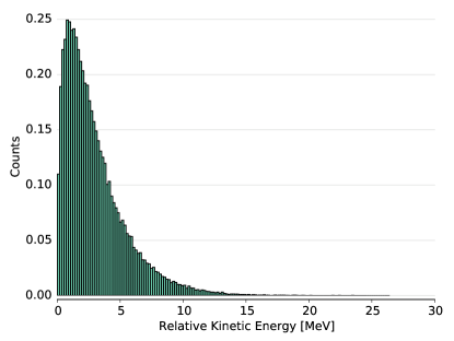
Figure 1: (Color online) Relative kinetic energy for pairs inside MST clusters.

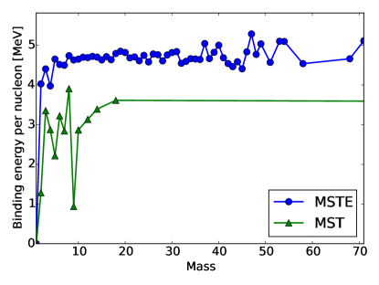
Figure 2: (Color online) Binding energy for MST and MSTE clusters. We can see that for every cluster size, MSTE clusters are more bound than MST ones.

3 Results

3.1 Clusters

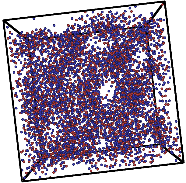
(a) $x=0.4,\,T=0.5\,\text{MeV}$

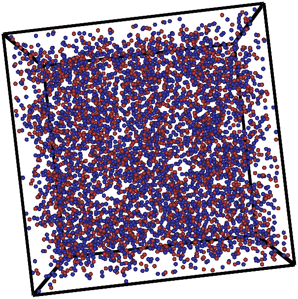
(b) $x=0.4,\,T=1.0\,\text{MeV}$

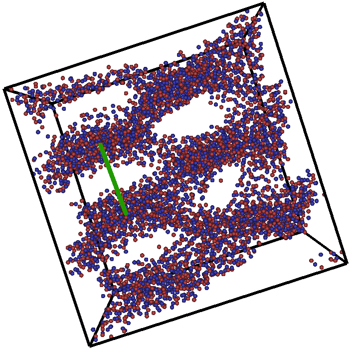
(c) $x=0.5,\,T=0.5\,\text{MeV}$

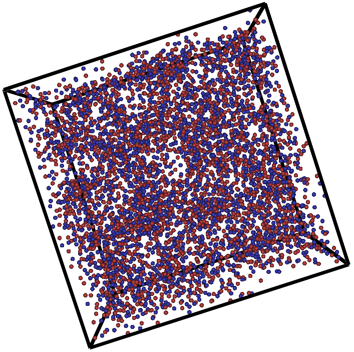
(d) $x=0.5,\,T=1.0\,\text{MeV}$

Figure 3: (Color online) Snapshots of a system with density $\rho=0.04\,\text{fm}^{-3}$ for different values of proton fraction and temperature, generated with VisIt [38]. Structures obtained at $T=0.5\,\text{MeV}$ differ substantially. Nevertheless both show inhomogeneities. We can see in panel 3(c) a green line marking a correlation length of $\approx 15\,\text{fm}$.

In figure 3 we show four different snapshots for proton fractions of $x=0.4$ and $x=0.5$ and temperature $T=0.5\,\text{MeV}$ and $T=1.0\,\text{MeV}$. We clearly see that the structures are no longer limited to those originally proposed by Ravenhall et al. [1]. To study them further we can see in figure 4 the corresponding cluster distribution according to MSTE algorithm. In this figure, we can see that for a proton fraction $x=0.2$ there are many isolated nucleons that are almost exclusively neutrons. These form the previously mentioned neutron gas that embeds the underlying proton structure.

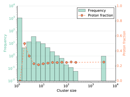
(a) $x=0.2$

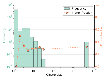
(b) $x=0.3$

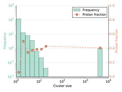
(c) $x=0.4$

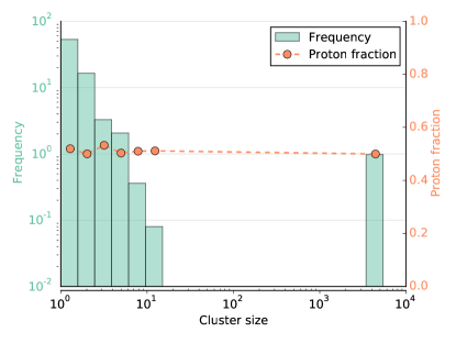
(d) $x=0.5$

Figure 4: (Color online) Cluster distribution with MSTE algorithm for temperature $T=2.0\,\text{MeV}$, density $\rho=0.04\,\text{fm}^{-3}$ and different proton fractions. For the lowest of the studied proton fractions, $x=0.2$, the large cluster has a higher proton fraction (about $30\%$ higher) and there are many isolated neutrons. Please note that the scales are different for each graph.

Another consequence of the neutron gas is that the proton fraction of the GNP structure is slightly higher than the proton fraction in the simulation cell. We can see from figure 4 that the proton fraction in the large cluster is about $x=0.24$, while the macroscopic proton fraction is $x=0.2$. In figure 5 we show the mass fraction of the largest cluster in terms of the temperature and the proton fraction, and note that even for very high temperatures ($T=2.0\,\text{MeV}$) a large cluster appears for every proton fraction. In particular, the smallest of the largest clusters contains more than $50\%$ of the total mass of the system.

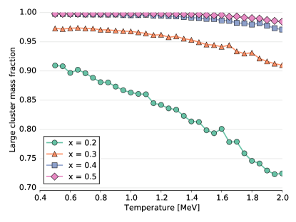
Figure 5: (Color online) Mass fraction of the largest cluster for $\rho=0.04\,\text{fm}^{-3}$ for different values of $x$.

3.2 Neutrino Opacity

As explained in Section 2.3.1, we calculate the neutrino opacity of the neutron rich matter. Figure 6 shows the pair distribution function, structure factor (see appendix for a detailed explanation of its calculation) and opacity for the gnocchi phase. In the pair distribution function we can identify (marked with $\color[rgb]{0,1,0}\blacktriangledown$) the peak that corresponds to the crystalline structure of the nucleons within the pasta — neutron correlation with nearest neighbors —, and also a very long range order (marked with a dashed line $\color[rgb]{1,0,0}-\,-$.); this interaction leads to the peak for low wavenumbers in the structure factor, related to the pasta structures. The structure factor displays a pasta peak (see Figure 6) located at $q_{\text{peak}}=0.37\,\text{fm}^{-1}$ (that translates to a neutrino energy of $E_{\nu}\approx 70\,\text{MeV}$) for this gnocchi phase and with a full width at half maximum of about $\Delta q_{\text{FWHM}}=0.08\,\text{fm}^{-1}$ ($\Delta E_{\text{FWHM}}\approx 15\,\text{MeV}$), by so defining a range of wavelengths in which the structure is considerably opaque.

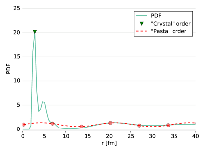
(a) Pair distribution function.

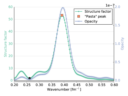
(b) Static structure factor.

Figure 6: (Color online) 6(a) Pair distribution function; and 6(b) static structure factor and opacity for a system with proton fraction $x=0.4$, density $\rho=0.01\,\text{fm}^{-3}$ and temperature $T=0.5\,\text{MeV}$. The first peak in the $g(r)$ due to crystalline structures is marked with $\color[rgb]{0,1,0}\blacktriangledown$, while the very long range order is marked with a dashed line $\color[rgb]{1,0,0}-\,-$. In the structure factor we can see the peak located at $q_{\text{peak}}=0.37\,\text{fm}^{-1}$ with a width of about $\text{FWHM}=0.08\,\text{fm}^{-1}$. The ripples for low wavenumbers are due to finite size effects.

We simulated the system for a total of about 1000 different configurations (4 different proton fractions, 10 different densities and 30 different temperatures). For each configuration of given proton fraction, density and temperature, we calculate the structure factor and calculate the corresponding opacity, according to equation (6) and extract its maximum value for long wavelengths. We will refer to this value as opacity peak. A word of caution must be said about the low temperatures. As we have shown in a previous work [16], below a certain temperature (near $1\,\text{MeV}$) the system might lock in one of many local minima. Because of this, the system cannot be directly simulated at low temperatures. Instead, the low temperature limit must be obtained coming from high temperatures, carefully lowering the temperature and checking whether the system is thermalized or not.

Figure 7 shows the opacity peak wavelength and opacity peak height for the lowest temperature studied in this work ($T=0.5\,\text{MeV}$) as a function of the density. We observe that the opacity peak wavelength decreases as the density increases, meaning that the correlation length of the structure is lower as the density increases. This is to be expected, since the higher the density, the closer the structures are. Nevertheless, we emphasize that the structure changes with the density, not only with transition in morphology (e. g. from spaghetti to lasagna) but also, for example, gnocchi clusters have different sizes for different densities. This interplay between the structures changing internally and also changing their spatial distribution is what results in the figure 7(a). We can see that the opacity peak wavelength changes rapidly for low densities (those of gnocchi), but tends to stabilize for the other pasta phases. Consider also that, since the $S(q)$ has a certain width near the peak, the structure would scatter neutrinos in a range of wavelengths that are near said maximum. Interestingly, the opacity peak height reaches its maximum for $\rho=0.01\,\text{fm}^{-3}$, where we still have gnocchi as can be evidenced by the cluster distributions in figure 8.

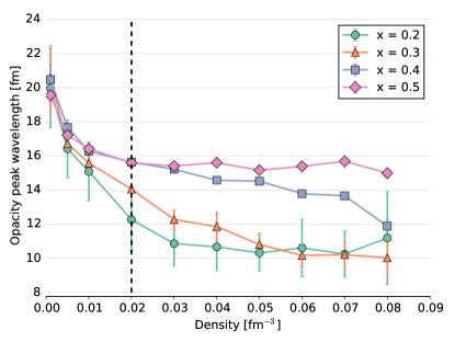
(a) Opacity peak wavelength

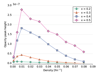
(b) Opacity peak height

Figure 7: (Color online) Opacity peak 7(a) wavelength and 7(b) height for low temperature ($T=0.5\,\text{MeV}$) as a function of density for different proton fractions. We can see the wavelength changing rapidly for $\rho<0.02\,\text{fm}^{-3}$ (gnocchi phase) and stabilizing for higher densities.

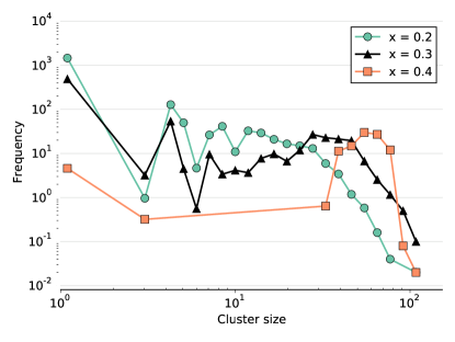
Figure 8: (Color online) Cluster distribution with MSTE algorithm for temperature $T=0.5\,\text{MeV}$, density $\rho=0.01\,\text{fm}^{-3}$ and different proton fractions. We can see that all of them have gnocchi mass distributions.

In figure 9 we show the opacity peak for the different thermodynamic configurations. We can see there that as the proton fraction decreases, the opacity decreases as well. For every proton fraction studied, the opacity peak falls rapidly for temperatures higher than $T=0.8\,\text{MeV}$, and it is about $1/4$ of the opacity peak at $T=0.5\,\text{MeV}$. The system opacity goes down as the proton fraction is reduced because the backbone structure is due to the proton long-range Coulomb interaction. When there is one neutron for each proton ($x=0.5$), the neutron structure follows almost identically that of the proton backbone. However, as the neutron proportion rises, the neutron structure is smeared out and its long range correlation begins to vanish. This effect can be seen in the cluster distribution for $x=0.2$, where we have many isolated neutrons, that are the embedding neutron gas. These characteristics affect the inhomogeneities that appear in $x=0.5$, suppressing their long range opacity.

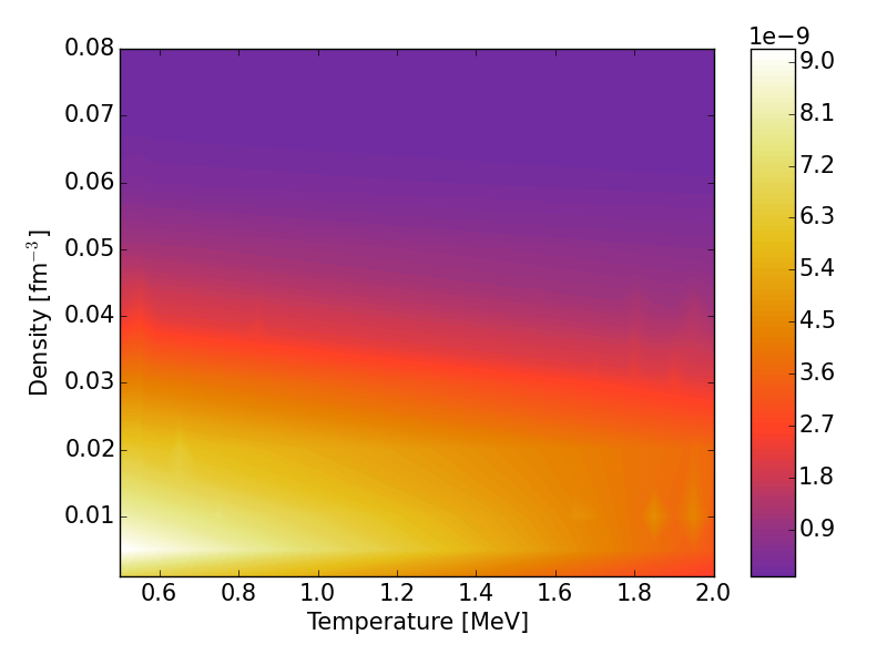
(a) $x=0.2$

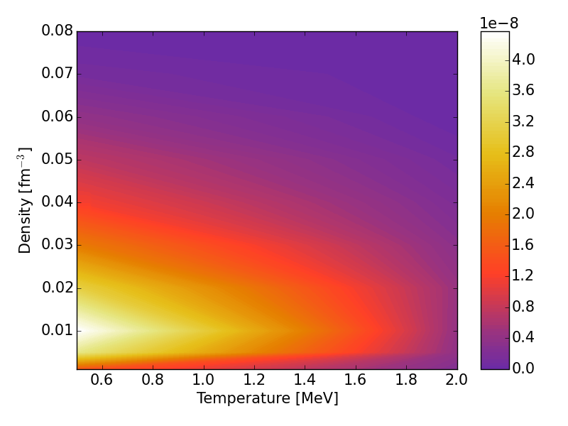
(b) $x=0.3$

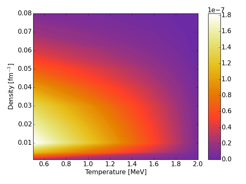
(c) $x=0.4$

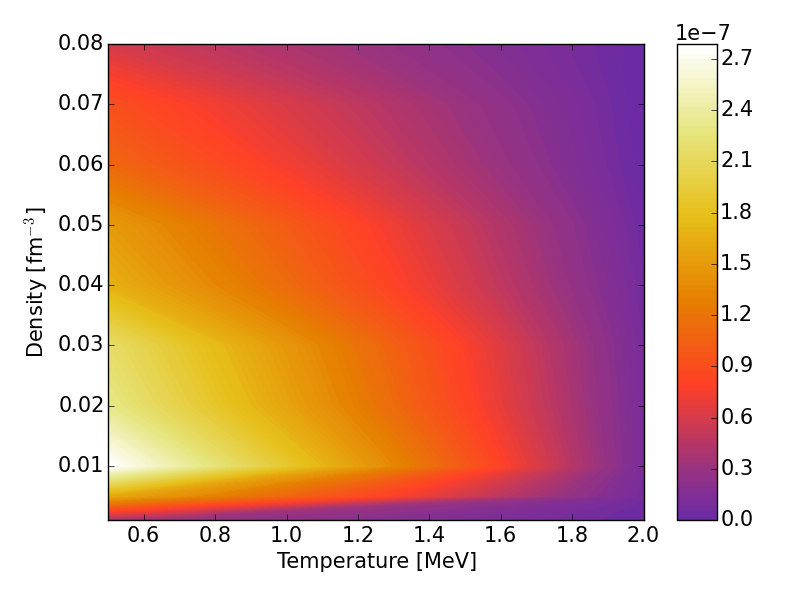
(d) $x=0.5$

Figure 9: (Color online) Opacity peak height in the very long wavelength for different proton fractions as a function of temperature and density. It can be seen that the opacity decreases drastically for $T\gtrsim 0.8\,\text{MeV}$. We also show here that the opacity is affected by the proton fraction, as it can be noted from the scales on the color bar. Also note that in the opacity for $x=0.2$ and $x=0.3$, the results are governed by noise.

From figure 5 we can see that even for very high temperatures ($T=2.0\,\text{MeV}$) a large cluster appears for every proton fraction. This large structure is the Generalized Nuclear Pasta, that is responsible for the long range interaction. The reason why the opacity gets drastically depressed as the temperature rises therefore is not because the large cluster disappears, but because of structural changes.

4 Discussion and Concluding Remarks

Neutron rich matter develops non-homogeneous structures (usually referred to as nuclear pasta) that strongly alter its opacity to neutrinos. By analyzing the behavior of the neutron-neutron static structure factor and radial distribution function over a wide range of densities, temperatures and proton fractions, we are able to calculate the wavelength at which maximum scattering takes place. We have seen that at high densities, where very big clusters are expected (spaghetti and lasagna), the wavelength stays relatively constant and the maximum opacity is obtained for rather energetic neutrinos ($E_{\nu}\approx 80\,\text{MeV}$, typical of a very early stage of the evolution of proto-neutron stars). As the density goes down, we move into the gnocchi pasta phase, in which clusters are of finite size. In this case, the maximum opacity moves to lower energies. As seen in figure 9 this increase on the opacity not only takes place when heterogeneities are of the commonly referred nuclear pasta, but also appears when these structures are quite deformed (the generalized nuclear pasta that we can see in figure 3).

We expect these results to be qualitatively correct, but quantitatively dependent on the model chosen to describe neutron rich matter. The model we are using in this work has been extensively studied in collisions and heavy ion physics; that is the reason why we have chosen it to describe quantitatively neutron rich matter.

Neutron rich matter hydrodynamic models [39, 40, 41, 42, 43] can yield proton fraction, density and temperature for different conditions (supernovae, proto-neutron stars, neutron stars). From this work, we are able to find, for this specific model, the neutrino opacity for different thermodynamic conditions. Therefore, combining these two results with eventual measurements of the neutrino opacity in neutron stars, we can check the validity of different nuclear models and, consequently, move a step forward towards finding the nuclear equation of state.

Appendix A On the calculation of the structure factor

The structure factor of a system is defined by the sample scattering amplitude [44]

$$\Psi(\mathbf{Q})=\frac{1}{\langle b\rangle}\sum_{i}b_{i}\text{e}^{i\mathbf{Q}\cdot\mathbf{R}_{i}}$$ (12)

with $\mathbf{Q}$ the diffraction vector or momentum transfer. $\mathbf{R}_{i}$ is the position of the particle $i$, and $\langle b\rangle$ is the average of the scattering amplitude of each particle in the vacuum $b_{i}$. From this moment on, we will consider that all of the atoms are of the same species, $b_{i}=b$.

From $\Psi(\mathbf{Q})$ we define the structure factor $S(\mathbf{Q})$ as

$$S(\mathbf{Q})=\frac{1}{N}|\Psi(\mathbf{Q})|^{2}$$ (13)

What follows immediately from this expression is that the structure function must be always positive for every value of $\mathbf{Q}$. We can expand the scattering amplitude and use $|z|=z\cdot z^{*}$ and, if all the atoms are of the same type,

$$S(\mathbf{Q}) =\frac{1}{N}\left(\sum_{i}\text{e}^{i\mathbf{Q}\cdot\mathbf{R}_{i}}\right)\left(\sum_{j}\text{e}^{-i\mathbf{Q}\cdot\mathbf{R}_{j}}\right)$$ (14)

$$=\frac{1}{N}\sum_{i,j}\text{e}^{i\mathbf{Q}\cdot(\mathbf{R}_{i}-\mathbf{R}_{j})}$$ (15)

$$=\frac{1}{N}\left[N+\sum_{i<j}\left(\text{e}^{i\mathbf{Q}\cdot(\mathbf{R}_{i}-\mathbf{R}_{j})}+\text{e}^{i\mathbf{Q}\cdot(\mathbf{R}_{i}-\mathbf{R}_{j})}\right)\right]$$ (16)

$$=1+\frac{2}{N}\sum_{i<j}\cos{\mathbf{Q}\cdot\mathbf{R}_{ij}}$$ (17)

Usually we are interested in the powder average of the structure factor. This is the structure factor averaged for every possible orientation of the diffraction vector - because in a powder we have a lot of structures randomly oriented. We calculate therefore

$$S(q)=\frac{1}{4\pi}\int\text{d}\phi\text{d}(\cos\theta)S(\mathbf{Q})$$ (18)

This integral can be performed easily if we put the $z$ axis along with the direction of $\mathbf{Q}$ and perform the integration by rotating the distances $\mathbf{R}_{ij}$

$$S(q) =\frac{1}{4\pi}\int\text{d}\phi\text{d}(\cos\theta)\left[1+2\sum_{i<j}\cos\left(q\,r_{ij}\,\cos\theta\right)\right]$$ (19)

$$=1+\frac{1}{2N}\int\text{d}(\cos\theta)2\sum_{i<j}\cos\left(q\,r_{ij}\,\cos\theta\right)$$ (20)

$$=1+\frac{1}{2N}2\sum_{i<j}\left.\frac{\sin(q\,r_{ij}u)}{q\,r_{ij}}\right|_{u=-1}^{u=1}$$ (21)

$$=1+\frac{2}{N}\sum_{i<j}\frac{\sin(q\,r_{ij})}{q\,r_{ij}}$$ (22)

This is the famous Debye formula and, since its the average of an always positive quantity, it must be always positive.

One of the most usual problems when we model and study systems in computer simulations is that we don’t have actual infinite systems. We do, however, use the periodic boundary conditions (PBC) usually to emulate the behavior of infinite systems. With the periodic boundary conditions we use the minimum image convention: from all the possible positions through the boundaries for particle $i$ and $j$, we pick whichever pair is closest. By using the above mentioned method for a very simple test case (a simple cubic 3D lattice with 4$\times$4$\times$4=64 atoms) we calculated the structure factor that can be seen in figure 10.

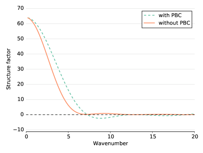
Figure 10: Comparison of structure factor with and without PBC.It’s evident that the structure factor calculated with periodic boundary conditions shows negative values, which should not exist from the definition of the structure factor.

We can see that the structure factor calculated with PBC attains negative values, even though those values ought to be forbidden. The reason for this behavior is the minimum image convention: the pair distance now isn’t always $r_{ij}=r_{j}-r_{i}$, but depends on whether we use the original particles or their images. Therefore, this “new” structure factor isn’t the product of two complex conjugate numbers. To explore the effect that the minimum image convention has on the structure factor, we show a comparison of the structure factor with and without boundary conditions (i. e., with the 64 atoms in a void) in figure 10.

This shows that the structure factor, when we use its definition without minimum image convention, is (as expected) always positive.

The question then, remains: how can we simulate an infinite medium when calculating structure factor? The first answer is that it is not that obvious that we would actually need this infinite medium, since the periodic images of the cell would be aligned in a crystal that might interfere with the structure within the cell — the one we actually do want to study. However, a couple of replicas should be enough to smear out the finite size effects. One of the possibilities is to replicate explicitly the box, creating the particles in the neighboring cells by duplication of the original ones. This, though, implies a calculation much harder, since the sum is over $N^{2}$ particles, and replicating only one cell right and left in each direction would imply a computational time of ${(3^{3}\cdot N)}^{2}\approx 700\cdot N^{2}$. In general, the complexity $\mathcal{O}(N^{2})$ makes structure factor calculation very expensive for large systems.

There is an alternative to add the boundary conditions. We begin with the definition of the sample scattering amplitude as in 12, but writing explicitly the periodic boundary images we want to consider:

$$\Psi(\mathbf{Q})=\sum_{i}\sum_{j}\text{e}^{i\mathbf{Q}\cdot(\mathbf{R}_{i}+\mathbf{\Delta L}_{j})}$$ (23)

where $\mathbf{\Delta L}_{j}$ is the distance between a particle and its $j$-th periodic replica. Since the sums are independent, we can write:

$$\Psi(\mathbf{Q})=\left(\sum_{i}\text{e}^{i\mathbf{Q}\cdot\mathbf{R}_{i}}\right)\left(\sum_{j}\text{e}^{i\mathbf{Q}\cdot\mathbf{\Delta L}_{j}}\right)$$ (24)

Multiplying by the conjugate gives us the structure factor

$$S(\mathbf{Q}) =\left|\sum_{i}\text{e}^{i\mathbf{Q}\cdot\mathbf{R}_{i}}\right|^{2}\left|\sum_{j}\text{e}^{i\mathbf{Q}\cdot\mathbf{\Delta L}_{j}}\right|^{2}$$ (25)

$$=S_{\text{cell}}(\mathbf{Q})\,S_{\text{PBC}}(\mathbf{Q})$$ (26)

The advantage of this calculation is that it is linear in the sum of the number of particles $N$ and the number of replicas $M$ consider, $\mathcal{O}(N+M)$, much lower than the previous $\mathcal{O}(N^{2}M^{2})$. Consequently, if we want to focus on a region of $\mathbf{Q}$, this new approach will be useful. We are left with only one detail, respecting the powder average. It is not trivial how to calculate this integral, since we need to give proper weights to each angle. In this work we used the Lebedev quadrature [45], although other methods like Importance Sampling Montecarlo can be useful in this situation.

References

- [1] D. G. Ravenhall, C. J. Pethick, and J. R. Wilson, “Structure of Matter below Nuclear Saturation Density,” Phys. Rev. Lett., vol. 50, pp. 2066–2069, June 1983.
- [2] M.-a. Hashimoto, H. Seki, and M. Yamada, “Shape of Nuclei in the Crust of Neutron Star,” Prog. Theor. Phys., vol. 71, pp. 320–326, Feb. 1984.
- [3] D. Page, J. M. Lattimer, M. Prakash, and A. W. Steiner, “Minimal Cooling of Neutron Stars: A New Paradigm,” ApJS, vol. 155, p. 623, Dec. 2004.
- [4] R. D. Williams and S. E. Koonin, “Sub-saturation phases of nuclear matter,” Nuclear Physics A, vol. 435, pp. 844–858, Mar. 1985.
- [5] K. Oyamatsu, “Nuclear shapes in the inner crust of a neutron star,” Nuclear Physics A, vol. 561, pp. 431–452, Aug. 1993.
- [6] C. P. Lorenz, D. G. Ravenhall, and C. J. Pethick, “Neutron star crusts,” Phys. Rev. Lett., vol. 70, pp. 379–382, Jan. 1993.
- [7] K. S. Cheng, C. C. Yao, and Z. G. Dai, “Properties of nuclei in the inner crusts of neutron stars in the relativistic mean-field theory,” Phys. Rev. C, vol. 55, pp. 2092–2100, Apr. 1997.
- [8] G. Watanabe, K. Iida, and K. Sato, “Thermodynamic properties of nuclear “pasta” in neutron star crusts,” Nuclear Physics A, vol. 676, pp. 455–473, Aug. 2000.
- [9] G. Watanabe and K. Iida, “Electron screening in the liquid-gas mixed phases of nuclear matter,” Phys. Rev. C, vol. 68, p. 045801, Oct. 2003.
- [10] K. Nakazato, K. Oyamatsu, and S. Yamada, “Gyroid Phase in Nuclear Pasta,” Phys. Rev. Lett., vol. 103, p. 132501, Sept. 2009.
- [11] T. Maruyama, K. Niita, K. Oyamatsu, T. Maruyama, S. Chiba, and A. Iwamoto, “Quantum molecular dynamics approach to the nuclear matter below the saturation density,” Phys. Rev. C, vol. 57, pp. 655–665, Feb. 1998.
- [12] T. Kido, T. Maruyama, K. Niita, and S. Chiba, “MD simulation study for nuclear matter,” Nuclear Physics A, vol. 663–664, pp. 877c–880c, Jan. 2000.
- [13] G. Watanabe, K. Sato, K. Yasuoka, and T. Ebisuzaki, “Structure of cold nuclear matter at subnuclear densities by quantum molecular dynamics,” Phys. Rev. C, vol. 68, p. 035806, Sept. 2003.
- [14] C. Horowitz, M. Pérez-García, J. Carriere, D. Berry, and J. Piekarewicz, “Nonuniform neutron-rich matter and coherent neutrino scattering,” Phys. Rev. C, vol. 70, p. 065806, Dec. 2004.
- [15] C. O. Dorso, P. A. Giménez Molinelli, and J. A. López, “Topological characterization of neutron star crusts,” Phys. Rev. C, vol. 86, p. 055805, Nov. 2012.
- [16] P. N. Alcain, P. A. Giménez Molinelli, and C. O. Dorso, “Beyond nuclear “pasta” : Phase transitions and neutrino opacity of new “pasta” phases,” Phys. Rev. C, vol. 90, p. 065803, Dec. 2014.
- [17] R. J. Lenk, T. J. Schlagel, and V. R. Pandharipande, “Accuracy of the Vlasov-Nordheim approximation in the classical limit,” Phys. Rev. C, vol. 42, pp. 372–385, July 1990.
- [18] C. Dorso, S. Duarte, and J. Randrup, “Classical simulation of the Fermi gas,” Physics Letters B, vol. 188, pp. 287–294, Apr. 1987.
- [19] C. Dorso and J. Randrup, “Classical simulation of nuclear systems,” Physics Letters B, vol. 215, pp. 611–616, Dec. 1988.
- [20] C. Hartnack, L. Zhuxia, L. Neise, G. Peilert, A. Rosenhauer, H. Sorge, J. Aichelin, H. Stöcker, and W. Greiner, “Quantum molecular dynamics a microscopic model from UNILAC to CERN energies,” Nuclear Physics A, vol. 495, pp. 303–319, Apr. 1989.
- [21] C. J. Horowitz, M. A. Pérez-García, and J. Piekarewicz, “Neutrino-“pasta” scattering: The opacity of nonuniform neutron-rich matter,” Phys. Rev. C, vol. 69, p. 045804, Apr. 2004.
- [22] A. Chernomoretz, L. Gingras, Y. Larochelle, L. Beaulieu, R. Roy, C. St-Pierre, and C. O. Dorso, “Quasiclassical model of intermediate velocity particle production in asymmetric heavy ion reactions,” Phys. Rev. C, vol. 65, p. 054613, May 2002.
- [23] J. A. López and C. Dorso, Lectures Notes on Phase Transformations in Nuclear Matter. WORLD SCIENTIFIC, Aug. 2000.
- [24] A. Barranon, C. O. Dorso, and J. A. Lopez, “Searching for criticality in nuclear fragmentation,” Revista mexicana de física, vol. 47, pp. 93–97, 2001.
- [25] C. O. Dorso and J. A. López, “Selection of critical events in nuclear fragmentation,” Phys. Rev. C, vol. 64, p. 027602, July 2001.
- [26] A. Barranón, R. Cárdenas, C. O. Dorso, and J. A. López, “The critical exponent of nuclear fragmentation,” APH N.S., Heavy Ion Physics, vol. 17, pp. 59–73, Jan. 2003.
- [27] A. Barrañón, C. O. Dorso, and J. A. López, “Time dependence of isotopic temperatures,” Nuclear Physics A, vol. 791, pp. 222–231, July 2007.
- [28] A. Barrañón, J. Roa, and J. López, “Entropy in the nuclear caloric curve,” Phys. Rev. C, vol. 69, p. 014601, Jan. 2004.
- [29] C. O. Dorso, C. R. Escudero, M. Ison, and J. A. López, “Dynamical aspects of isoscaling,” Phys. Rev. C, vol. 73, p. 044601, Apr. 2006.
- [30] C. A. Dorso, P. A. G. Molinelli, and J. A. López, “Isoscaling and the nuclear EoS,” J. Phys. G: Nucl. Part. Phys., vol. 38, p. 115101, Nov. 2011.
- [31] S. Plimpton, “Fast Parallel Algorithms for Short-Range Molecular Dynamics,” Journal of Computational Physics, vol. 117, pp. 1–19, Mar. 1995.
- [32] W. M. Brown, A. Kohlmeyer, S. J. Plimpton, and A. N. Tharrington, “Implementing molecular dynamics on hybrid high performance computers – Particle–particle particle-mesh,” Computer Physics Communications, vol. 183, pp. 449–459, Mar. 2012.
- [33] A. L. Fetter and J. D. Walecka, Quantum Theory of Many-particle Systems. Courier Dover Publications, 2003.
- [34] P. N. Alcain, P. A. Giménez Molinelli, J. I. Nichols, and C. O. Dorso, “Effect of Coulomb screening length on nuclear “pasta” simulations,” Phys. Rev. C, vol. 89, p. 055801, May 2014.
- [35] H. Sonoda, G. Watanabe, K. Sato, T. Takiwaki, K. Yasuoka, and T. Ebisuzaki, “Impact of nuclear “pasta” on neutrino transport in collapsing stellar cores,” Phys. Rev. C, vol. 75, p. 042801, Apr. 2007.
- [36] C. Dorso and J. Randrup, “Early recognition of clusters in molecular dynamics,” Physics Letters B, vol. 301, pp. 328–333, Mar. 1993.
- [37] C. O. Dorso and P. E. Balonga, “Fluctuation dynamics of fragmenting spherical nuclei,” Phys. Rev. C, vol. 50, pp. 991–995, Aug. 1994.
- [38] H. Childs, E. S. Brugger, K. S. Bonnell, J. S. Meredith, M. Miller, B. J. Whitlock, and N. Max, “A Contract-Based System for Large Data Visualization,” in Proceedings of IEEE Visualization 2005, (Minneapolis, Minnesota), pp. 190–198, 2005.
- [39] M. Ruffert, H.-T. Janka, and G. Schaefer, “Coalescing Neutron Stars – a Step Towards Physical Models. I. Hydrodynamic Evolution and Gravitational-Wave Emission,” arXiv:astro-ph/9509006, Sept. 1995. arXiv: astro-ph/9509006.
- [40] A. Mezzacappa, A. C. Calder, S. W. Bruenn, J. M. Blondin, M. W. Guidry, M. R. Strayer, and A. S. Umar, “An Investigation of Neutrino-driven Convection and the Core Collapse Supernova Mechanism Using Multigroup Neutrino Transport,” ApJ, vol. 495, p. 911, Mar. 1998.
- [41] U. Geppert, M. Küker, and D. Page, “Temperature distribution in magnetized neutron star crusts,” Astronomy & Astrophysics, vol. 426, no. 1, p. 11, 2004.
- [42] S. Woosley and T. Janka, “The physics of core-collapse supernovae,” Nature Physics, vol. 1, pp. 147–154, Dec. 2005.
- [43] M. Liebendörfer, M. Rampp, H.-T. Janka, and A. Mezzacappa, “Supernova Simulations with Boltzmann Neutrino Transport: A Comparison of Methods,” ApJ, vol. 620, p. 840, Feb. 2005.
- [44] T. Egami and S. J. L. Billinge, Underneath the Bragg Peaks, Volume 16: Structural Analysis of Complex Materials. Pergamon, 1 edition ed., Oct. 2003.
- [45] V. I. Lebedev, “Values of the nodes and weights of ninth to seventeenth order gauss-markov quadrature formulae invariant under the octahedron group with inversion,” USSR Computational Mathematics and Mathematical Physics, vol. 15, no. 1, pp. 44–51, 1975.