Minimally non-local nucleon-nucleon potentials with chiral two-pion exchange including $\Delta$’s

M. Piarullia, L. Girlandab,c, R. Schiavilla${}^{\,{\rm a,d}}$, R. Navarro Pérez${}^{\,{\rm e}}$, J.E. Amaro${}^{\,{\rm e}}$, and E. Ruiz Arriola${}^{\,{\rm e}}$ ${}^{\,{\rm a}}$Department of Physics, Old Dominion University, Norfolk, VA 23529, USA
${}^{\,{\rm b}}$Department of Mathematics and Physics, University of Salento, I-73100 Lecce, Italy
${}^{\,{\rm c}}$INFN-Lecce, I-73100 Lecce, Italy
${}^{\,{\rm d}}$Theory Center, Jefferson Lab, Newport News, VA 23606, USA
${}^{\,{\rm e}}$Departamento de Física Atómica, Molecular y Nuclear and Instituto Carlos I de Física Teórica y Computacional
Universidad de Granada, E-18071 Granada, Spain
Abstract

We construct a coordinate-space chiral potential, including $\Delta$-isobar intermediate states in its two-pion-exchange component up to order $Q^{3}$ ($Q$ denotes generically the low momentum scale). The contact interactions entering at next-to-leading and next-to-next-to-next-to-leading orders ($Q^{2}$ and $Q^{4}$, respectively) are rearranged by Fierz transformations to yield terms at most quadratic in the relative momentum operator of the two nucleons. The low-energy constants multiplying these contact interactions are fitted to the 2013 Granada database, consisting of 2309 $pp$ and 2982 $np$ data (including, respectively, 148 and 218 normalizations) in the laboratory-energy range 0–300 MeV. For the total 5291 $pp$ and $np$ data in this range, we obtain a $\chi^{2}$/datum of roughly 1.3 for a set of three models characterized by long- and short-range cutoffs, $R_{\rm L}$ and $R_{\rm S}$ respectively, ranging from $(R_{\rm L},R_{\rm S})=(1.2,0.8)$ fm down to $(0.8,0.6)$ fm. The long-range (short-range) cutoff regularizes the one- and two-pion exchange (contact) part of the potential.

pacs:
13.75.Cs,21.30.-x,21.45.Bc

I Introduction

The nucleon-nucleon ($NN$) interaction is a basic building block in nuclear physics as it makes it possible to describe nuclear structure and nuclear reactions. If the forces were known accurately and precisely, the nuclear many-body problem would become a large-scale computation where precision and accuracy are defined in terms of the preferred numerical method. However, the lack of direct knowledge of the forces among constituents at separation distances relevant for nuclear structure and reactions drastically changes the rules of the game. Indeed, the use of a large but finite body of scattering data below a given maximal energy to provide constraints on the interaction transforms the whole setup into a statistical inference problem, based on the conventional least $\chi^{2}$-method. This fact was recognized already in 1957 Stapp:1956mz (see Ref. arndt1966chi for an early review) and, after many years, culminated in the admirable Nijmegen partial wave analysis (PWA) of 1993 Stoks93 , based on the crucial observations that charge-dependent one-pion-exchange (CD-OPE), tiny but essential electromagnetic and relativistic effects, and a judicious selection of the scattering database could actually provide a satisfactory fit with $\chi^{2}/{\rm datum}\sim 1$ for a total number of data consisting, as of 1993, of 1787 $pp$ and 2514 $np$ (normalizations included) at the $3\,\sigma$ level. These criteria have set the standard for PWA’s and the design of high quality phenomenological potentials Stoks94 ; Wiringa95 ; Rentmeester:1999vw ; Machleidt:2000ge ; Rentmeester:2003mf ; Gross08 ; Navarro13 ; Perez:2013oba ; Navarro14 . The inference point of view is mainly phenomenological and requires a balanced interplay between which data qualify as constraints and which models provide the most likely description of the data. None of these choices is free of prejudices and they are actually intertwined; a circumstance that should be kept in mind when assessing the reliability and predictive power of the theory aiming at a faithful representation of the input data and their uncertainties.

The quantum mechanical nature of the PWA with a given cutoff in energy leads to inverse scattering ambiguities which increase at short distances (see, for example, Refs. Inverse ; Baye:2014oea and references therein). Remarkably, a universal and model-independent low-energy interaction arises when unobserved high energy components above the cutoff are explicitly integrated out of the Hilbert space preserving the scattering amplitude Bogner:2001gq ; Bogner:2003wn . While this $V_{\rm low-k}$ framework is an extremely appealing setup based on Wilsonian renormalization, to date this universal interaction has not been determined from data directly and one has to proceed via a fitted and bare $NN$ interaction since off-shellness is required Arriola:2014fqa . However, inferring a $NN$ interaction from data, is not the full story, and three-nucleon, and possibly higher multi-nucleon, interactions are needed to describe residual contributions to nuclear binding energies Carlson2014 . As is well known, their strength and form are also affected by the chosen off-shell behavior of the $NN$ interaction and a universal $V_{\rm low-k}$ three-nucleon interaction remains to be found.

In an ideal situation all steps in the inference process, including the scattering data selection itself, should be carried out with the “true” theory, which for nuclear physics is quantum chromodynamics (QCD), the fundamental theory of interacting quarks and gluons. Assuming, as we do, that the theory is correct, QCD would just tell us which experiments are right and which are wrong, or whether the reported uncertainties are realistic with a given confidence level on the side of the experiment. At the same time one would set constraints on the QCD parameters such as the light quark masses and $\Lambda_{\rm QCD}$, or equivalently the pion mass $m_{\pi}$ and the pion weak decay constant $F_{\pi}$. While there has been impressive progress in bringing lattice QCD simulations for light quarks closer to nuclear physics working conditions (see Refs. Hatsuda:2012hw ; Detmold:2015jda and references therein), we do not yet envisage, at least not in the near future, the realization of conditions that would allow one to establish, on QCD grounds, the correctness of the about 8000 currently available published $pp$ and $np$ scattering data below pion production threshold. Instead, already in the early 90’s the phenomenological analysis carried out by the Nijmegen group made it possible to pin down the pion masses with a precision of 1 MeV from their PWA of $pp$ and $np$ data Klomp:1991vz .

In practice, we must content ourselves with an approximation scheme to the true theory in conjunction with a phenomenological approach. This specifically means assuming a sufficiently flexible parametrization of the interaction in terms of the relevant degrees of freedom which does not overlook some relevant physical feature. In what follows it is instructive to briefly review both the process and criteria taken into account to select a consistent database as well as the QCD-based theory used to describe it. Our aim is to make the reader aware of all the fine details which are needed in order to credibly falsify the theoretical model, QCD grounded or not, against the data and keep an open mind about the out-coming result.

On the theoretical side, we will assume along with Weinberg Weinberg:1990rz that there is a chiral effective field theory ($\chi$EFT) capable of systematically describing the strong interactions among nucleons, $\Delta$-isobars, and pions, as well as the electroweak interactions of these hadrons with external (electroweak) fields. In the specific case of two nucleons, the requirements imposed by $\chi$EFT can be incorporated into a non-relativistic quantum mechanical potential, constructed by a perturbative matching, order by order in the chiral expansion, between the on-shell scattering amplitude and the solution of the Schrödinger equation (see, for example, the review paper by Machleidt and Entem Entem11 ). Such a theory provides the most general scheme accommodating all possible interactions compatible with the relevant symmetries of QCD at low energies, in particular chiral symmetry. By its own nature, $\chi$EFT needs to be organized within a given power counting scheme and the resulting chiral potentials can conveniently be separated into long- and short-distance contributions, the latter (short-distance ones) featuring the needed counter-terms for renormalization. At leading order in the chiral expansion one has the venerable one-pion-exchange (OPE) potential which, as already mentioned, emerges as a universal and indispensable long-distance feature for an accurate description of proton-proton and neutron-proton scattering data Stoks93 . Higher orders in the chiral expansion incorporate the two-pion-exchange (TPE) potential Kaiser:1997mw , due to leading and sub-leading $\pi N$ couplings (the sub-leading couplings $c_{1}$, $c_{3}$, and $c_{4}$ can consistently be obtained from low energy $\pi N$ scattering data). The inclusion of TPE allows one to reduce the short-range cutoff separating long- and short-distance contributions, which helps in reducing the impact of details in the unknown short-distance behavior of the potentials. Nonetheless, we will note in Sec. IV that uncertainties are dominated by this diffuse separation between short and long distances.

There are many practical advantages deriving from a $\chi$EFT that explicitly includes $\Delta$-isobar degrees of freedom, the most immediate one being a numerical consistency between the values of the low-energy constants $c_{1}$, $c_{3}$ and $c_{4}$ inferred from either $\pi N$ or $NN$ scattering. Such a theory also naturally leads to three-nucleon forces induced by TPE with excitation of an intermediate $\Delta$ (the Fujita-Miyazawa three-nucleon force) as well as to two-nucleon electroweak currents (see for example Ref. Pastore2008 ). In addition, there are rather strong indications from phenomenology that $\Delta$ isobars play an important role in nuclear structure and reactions. An illustration of this are the three-nucleon forces involving excitation of intermediate $\Delta$’s, needed to reproduce the observed energy spectra and level ordering of low-lying states in s- and p-shell nuclei or the correct spin-orbit splitting of P-wave resonances in low-energy $n$-$\alpha$ scattering (for a review, see Ref. Carlson2014 ). Another illustration is the relevance of electroweak $N$-to-$\Delta$ transition currents in radiative and weak capture processes involving few-nucleon systems Schiavilla92 , specifically the radiative captures of thermal neutrons on deuteron and 3He Viviani96 ; Girlanda10 or the weak capture of protons on 3He (the so-called $hep$ process) Marcucci01 . It is for these reasons that in the present work we construct a minimally non-local coordinate space chiral potential, that includes $\Delta$ intermediate states in its TPE component—it is described in detail in Sec. II. Such a coordinate-space representation offers many computational advantages for ab initio calculations of nuclear structure and reactions, in particular for the type of quantum Monte Carlo calculations of s- and p-shell nuclei very recently reviewed in Ref. Carlson2014 .

On the experimental side, there are currently $\sim 8000$ published $pp$ and $np$ scattering data below pion production threshold corresponding to 24 different scattering observables, including differential cross sections, spin asymmetries, and total cross sections Bystricky1 ; Bystricky2 , see Ref. Navarro14 for updated $pp$ and $np$ abundance plots in the $(E_{\rm lab},\theta_{\rm cm})$ plane. However, not all of these data are mutually compatible and a decision has to be made as to which are more likely to be correct. In principle, the $NN$ scattering amplitude can be determined uniquely, provided a complete set of experiments is given—a rare situation for the case under consideration. Therefore, a theoretical model is needed to provide a smooth energy dependence which allows one to interpolate between different energy values, and helps in deciding on the mutual consistency of nearby data in $(E_{\rm lab},\theta_{\rm cm})$ plane. The PWA carried out in Granada parametrizes Navarro13 111The Granada database is located in the HADRONICA website http://www.ugr.es/~amaro/hadronica/. the interaction, for inter-nucleon distances $r$ less than 3 fm, in terms of a set equidistant delta-shells separated by $\Delta r=0.6$ fm (in other words, a coarse-grained parametrization), while retaining only the OPE component for $r>3$ fm. The choice of $\Delta r$ corresponds to the shortest de Broglie wavelength at about pion production threshold, and consequently all the data are weighted with their quoted experimental uncertainty. The result of the analysis has been a $3\,\sigma$ self-consistent database comprising a total of 6713 $pp$ and $np$ scattering data. More details on the data analysis specific to our potential are presented in Sec. III. One important aspect of the Granada PWA is the correlation pattern among the fitting parameters, namely different partial waves are mostly uncorrelated which, together with the large number of selected data, speaks in favor of a lack of bias in the selection process. Actually the correlation length which decides on the specific form of the potential should be smaller than the distance $\Delta r=0.6$ fm in the coarse-grained parametrization.

Chiral potentials have been subjected to PWA and confronted to $pp$ and $np$ scattering data up to lab energy of 350 MeV. Within the $\chi$EFT framework the Nijmegen group used the TPE potential Kaiser:1997mw to carry out $pp$ Rentmeester:1999vw and $np+pp$ Rentmeester:2003mf analyses determining the chiral constants $c_{3}$ and $c_{4}$ from these data while constraining $c_{1}$ from $\pi N$ data. Taking the chiral constants from $\pi N$ analyses, Entem and Machleidt Entem03 used a next-to-next-to-next-to-leading order (N3LO or $Q^{4}$, $Q$ generically specifying the low momentum scale) chiral potential to fit $pp$ and $np$ scattering data up to lab energy of 290 MeV. The resulting $\chi^{2}$/datum were 1.1 for 2402 $np$ data and 1.50 for 2057 $pp$ data, and consequently a global $\chi^{2}$/datum of 1.28. The chiral TPE potential Kaiser:1997mw was also used within the coarse grained framework to determine the chiral constants in Ref. Perez:2013oba with a global $\chi^{2}$/datum of 1.07, based on 6713 $pp$ and $np$ scattering data.

Other available chiral potentials Epelbaum:2004fk ; Entem2015 have not been confronted to scattering data directly but rather to phase shifts obtained in the Nijmegen analysis (the recent upgrade Epelbaum:2014efa of Ref. Epelbaum:2004fk relies on the same procedure, while in Ref. Entem2015 a study of peripheral phase shifts is carried out with two- and three-pion exchange potentials up to order $Q^{5}$). As we will show in Sec. IV, there is a substantial difference between fitting scattering data and fitting phase shifts mainly because of the existing correlations among the many partial waves and mixing angles. Actually, a good $\chi^{2}$-fit to phase shifts may yield quite a bad $\chi^{2}$ in a fit to data. Moreover, the spread in phase-shift values among different high-quality potentials fitting the same data reflects the differences in the potential representation and turns out to be larger than the estimated statistical errors (compare Fig. 1 of Ref. NavarroPerez:2012vr with Fig. 3 of Ref. Perez:2014jsa ). The consequences of these larger errors have been discussed in Ref. Perez:2013za .

The previous comments address the use of chiral potentials to fit selected $NN$ scattering databases which have been obtained from phenomenological representations of the interactions. An obvious question which comes to mind is whether chiral potentials, being credible and general low energy representations of QCD in the $NN$ sector, should be used themselves to select the database. Within the coarse grained framework the impact of chiral interactions on the selection of the database has also been studied in Ref. Perez:2013oba . The result was that a larger number of data were rejected but at the same time the number of parameters was reduced. This poses the interesting question on what is the meaning of improvement—a particularly critical issue when the potential itself (chiral or not) must be tested against the selected data. Obviously an incorrect model will appear to be correct if a sufficiently large number of data is discarded. However, the theory with just delta-shells+OPE is more general than that with delta-shells+(OPE+TPE), and hence data selection based on the former is more reliable. In any case, the results of Ref. Perez:2013oba show also that the long range part of the next-to-next-to-leading order (N2LO or $Q^{3}$) chiral potential can indeed fit the delta-shells+OPE selected data satisfactorily with a $\chi^{2}$/datum of 1.07, when the potential is taken to be valid for inter-nucleon distances ranging from 1.8 fm outwards.

The present paper is organized as follows. In the next section we describe the potential, while in Sec. III we provide a brief discussion of the data fitting. In Sec. IV we report the $\chi^{2}$ values obtained in the fits as well as the values for the low-energy constants that characterize the potential, and show the calculated phase shifts for the lower partial waves (S, P, and D waves) and compare them to those from recent PWA’s. There, we also provide tables of the $pp$, $np$ and $nn$ effective range parameters and of deuteron properties, including a figure of the deuteron S and D waves. Finally, in Sec. V we summarize our conclusions. A number of details are relegated to Appendices A-E.

II Potentials

The two-nucleon potential includes a strong interaction component derived from χ𝜒\chiEFT up to next-to-next-to-next-to-leading order (N3LO or Q4superscript𝑄4Q^{4}) and denoted as v12subscript𝑣12v_{12}, and an electromagnetic interaction component, including up to terms quadratic in the fine structure constant α𝛼\alpha (first and second order Coulomb, Darwin-Foldy, vacuum polarization, and magnetic moment interactions), and denoted as v12EMsuperscriptsubscript𝑣12EMv_{12}^{\rm EM}. The v12EMsuperscriptsubscript𝑣12EMv_{12}^{\rm EM} component is the same as that adopted in the Argonne v18subscript𝑣18v_{18} (AV18) potential Wiringa95 . The component induced by the strong interaction is separated into long- and short-range parts, labeled, respectively, v12Lsuperscriptsubscript𝑣12Lv_{12}^{\rm L} and v12Ssuperscriptsubscript𝑣12Sv_{12}^{\rm S}. The v12Lsuperscriptsubscript𝑣12Lv_{12}^{\rm L} part includes the one 
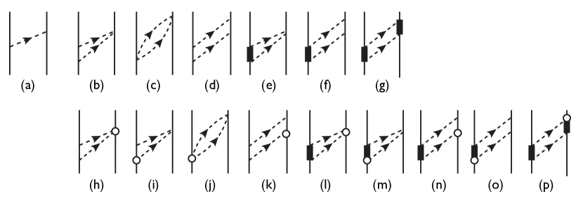
pion-exchange (OPE) and two pion-exchange (TPE) contributions, illustrated in Fig. 1: panel (a) represents the OPE contribution at leading order (LO or Q0superscript𝑄0Q^{0}); panels (b)-(g) represent the TPE contributions at next-to leading order (NLO or Q2superscript𝑄2Q^{2}) without and with ΔΔ\Delta-isobars in the intermediate states; lastly, panels (h)-(p) represent sub-leading TPE contributions at next-to-next-to leading order (N2LO or Q3superscript𝑄3Q^{3}). The NLO and N2LO loop corrections contain ultraviolet divergencies, which are isolated in dimensional regularization and then reabsorbed into contact interactions by renormalization of the associated low energy constants (LEC’s) Epelbaum98 ; Pastore09 . Additional loop corrections at NLO and N2LO only lead to renormalization of OPE and contact interactions Epelbaum98 ; Viviani14 , and will not be discussed any further here.

Refer to caption
Figure 1: OPE and TPE contributions at LO [(a)], NLO [(b)-(g)], and N2LO [(h)-(p)]. Nucleons, $\Delta$ isobars, and pions are denoted, respectively, by the solid, thick-solid, and dashed lines; both direct and crossed box contributions are retained in diagrams (d), (f)-(g), (k), (n)-(p). The open circles denote $\pi N$ and $\pi N\Delta$ couplings from the sub-leading chiral Lagrangians $\mathcal{L}_{\pi N}^{(2)}$ Fettes00 and $\mathcal{L}_{\pi N\Delta}^{(2)}$ Krebs07 . Note that relativistic $1/M_{N}$-corrections ($M_{N}$ is the nucleon mass) included in $\mathcal{L}_{\pi N}^{(2)}$ Lagrangian are not considered here. In particular the contributions of diagrams (i), (k) and (n) are neglected.
Table 1: Values of (fixed) low energy constants (LEC’s): $g_{A}$ and $h_{A}=3\,g_{A}/\sqrt{2}$ are adimensional, $F_{\pi}=2\,f_{\pi}$ is in MeV, and the remaining LEC’s are in GeV-1.
$g_{A}$ $h_{A}$ $F_{\pi}$ $c_{1}$ $c_{2}$ $c_{3}$ $c_{4}$ $b_{3}+b_{8}$
$1.29$ $2.74$ $184.80$ $-0.57$ $-0.25$ $-0.79$ $1.33$ $1.40$

The LO, NLO, and N2LO terms are well known, and explicit expressions for them can be found in Refs. Epelbaum98 ; Pastore09 ; Kaiser1998 ; Epelbaum04 ; Krebs07 . The LO and NLO terms depend on the the pion decay amplitude $F_{\pi}$, and the nucleon and $N$-to-$\Delta$ axial coupling constants, respectively $g_{A}$ and $h_{A}=3\,g_{A}/\sqrt{2}$ (this value for $h_{A}$ is from the large $N_{c}$ expansion or strong-coupling model Green76 , and is in good agreement with the value inferred from the empirical $\Delta$-width). The sub-leading N2LO terms also depend on the LEC’s $c_{1}$, $c_{2}$, $c_{3}$, and $c_{4}$ and the combination of LEC’s $(b_{3}+b_{8})$, respectively from the second order $\pi N$ and $\pi N\Delta$ chiral Lagrangians $\mathcal{L}_{\pi N}^{(2)}$ Fettes00 and $\mathcal{L}_{\pi N\Delta}^{(2)}$ Krebs07 . The values of these LEC’s, as determined by fits to $\pi N$ scattering data Krebs07 , and of the masses and other physical constants adopted in the present study are listed in Tables 1 and 2.

Table 2: Values of charged and neutral pion masses, proton and neutron masses, $\Delta$-nucleon mass difference, and electron mass (all in MeV), and of the (adimensional) fine structure constant $\alpha$. Note that $\hbar c$ is taken as 197.32697 MeV fm.
$m_{\pi_{0}}$ $m_{\pi_{\pm}}$ $M_{n}$ $M_{p}$ $\Delta M$ $m_{e}$ $\alpha^{-1}$
$134.9766$ $139.5702$ $939.56524$ $938.27192$ $293.1$ $0.510999$ $137.03599$

In the static limit, the momentum-space LO, NLO, N2LO terms are functions of the momentum transfer ${\bf k}$; hereafter, we define ${\bf k}={\bf p}^{\prime}-{\bf p}$ and ${\bf K}=({\bf p}^{\prime}+{\bf p})/2$, where ${\bf p}$ and ${\bf p}^{\prime}$ are the initial and final relative momenta of the two nucleons. Coordinate-space expressions for the TPE terms are obtained by using the spectral function representation Epelbaum04 , however with no spectral cutoff 222This detail is important, since the lack of a spectral cutoff ensures the correct analytical properties of the partial wave scattering amplitude in the complex $p_{\rm cm}$ plane, namely the proper branch-cut structure of the TPE potential with the opening of the left cut at $p_{\rm cm}=\pm i\,m_{\pi}$. Moreover, it produces the correct asymptotic behavior of the potential avoiding mid-range distortions. We refer to Refs. Valderrama:2008kj ; PavonValderrama:2010fb for a discussion of these issues. As a matter of fact, the N3LO-$\not{\Delta}$ upgrade in Ref. Epelbaum:2014efa improves over the work in Ref. Epelbaum:2004fk by removing the spectral cutoff.,

$$v_{\rm L}^{l,{\rm TPE}}(r)\!=\!\frac{1}{2\pi^{2}r}\int_{2m_{\pi}}^{\infty}d\mu\,\mu\,e^{-\mu r}f^{l}(\mu)\,{\rm Im}[\,\widetilde{v}_{\rm L}^{\,l,{\rm TPE}}(0^{+}-i\mu)\,]\,,$$ (1)

in terms of the left-cut discontinuity at $k=0^{+}-i\,\mu$. Here $f^{c}(\mu)=f^{\tau}(\mu)=1$, $f^{\sigma}(\mu)=f^{\sigma\tau}(\mu)=2/3$ and $f^{t}(\mu)=f^{t\tau}(\mu)=-(3+3\mu r+\mu^{2}r^{2})/(3\,r^{2})$, and the functions $\widetilde{v}_{\rm L}^{\,l,{\rm TPE}}(k)$ are the momentum-space TPE components of the potential at NLO and N2LO,

$$\widetilde{v}_{12}^{\,{\rm L,TPE}}=\sum_{l=1}^{6}\widetilde{v}_{\rm L}^{\,l,{\rm TPE}}(k)\,\widetilde{O}^{\,l}_{12}\ ,$$ (2)

with $\widetilde{O}^{l=1,\dots,6}_{12}=[{\bf 1}\,,\,{\bm{\sigma}}_{1}\cdot{\bm{\sigma}}_{2}\,,\,{\bm{\sigma}}_{1}\cdot{\bf k}\,\,{\bm{\sigma}}_{2}\cdot{\bf k}]\otimes[{\bf 1}\,,\,{\bm{\tau}}_{1}\cdot{\bm{\tau}}_{2}]$ denoted as $c,\tau,\sigma,\sigma\tau,t,t\tau$. Those corresponding to diagrams (b)-(d) and (h)-(k) in Fig. 1 are known in closed form (see, for example, Ref. Epelbaum04 ) and are listed in Appendix A for completeness; the remaining ones corresponding to diagrams (e)-(g) and (l)-(p) have been derived in terms of a parametric integral, and they too are given in Appendix A. The radial functions $v_{\rm L}^{l}(r)$ are singular at the origin (they behave as $1/r^{n}$ with $n$ taking on values up to $n=6$, see Refs. Valderrama:2008kj ; PavonValderrama:2010fb for analytical expressions), and each is regularized by a cutoff of the form

$$C_{R_{\rm L}}(r)=1-\frac{1}{(r/R_{\rm L})^{6}\,e^{(r-R_{\rm L})/a_{L}}+1}\ ,$$ (3)

where in the present work three values for the radius $R_{L}$ are considered $R_{L}=(0.8,1.0,1.2)$ fm with the diffuseness $a_{L}$ fixed at $a_{L}=R_{L}/2$ in each case. The potential $v_{12}^{\rm L}$, including the well known OPE components at LO regularized by the cutoff in Eq. (3), then reads in coordinate space

$$v_{12}^{\rm L}=\left[\sum_{l=1}^{6}v_{\rm L}^{l}(r)\,O^{l}_{12}\right]+v_{\rm L}^{\sigma T}(r)\,O^{\sigma T}_{12}+v_{\rm L}^{tT}(r)\,O^{tT}_{12}\ ,$$ (4)

where

$$O^{l=1,...,6}_{12}=\left[{\bf 1}\,,\,{\bm{\sigma}}_{1}\cdot{\bm{\sigma}}_{2}\,,\,S_{12}\right]\otimes\left[{\bf 1}\,,\,{\bm{\tau}}_{1}\cdot{\bm{\tau}}_{2}\right]\ ,$$ (5)

$O^{\sigma T}_{12}={\bm{\sigma}}_{1}\cdot{\bm{\sigma}}_{2}\,T_{12}$, and $O^{tT}_{12}=S_{12}\,T_{12}$, and $T_{12}=3\,\tau_{1z}\tau_{2z}-{\bm{\tau}}_{1}\cdot{\bm{\tau}}_{2}$ is the isotensor operator. The terms proportional to $T_{12}$ account for the charge-independence breaking induced by the difference between the neutral and charged pion masses in the OPE. However, this difference is ignored in the NLO and N2LO loop corrections which have been evaluated with $m_{\pi}=\left(2\,m_{\pi^{+}}+m_{\pi^{0}}\right)/3$. Additional (and small) isospin symmetry breaking terms arising from OPE Friar04 and TPE Epelbaum05 and from OPE and one-photon exchange Kolck98 ; Kaiser06 have also been neglected.

The potential $v_{12}^{\rm S}$ includes charge-independent (CI) contact interactions at LO, NLO and N3LO, and charge-dependent (CD) ones at LO and NLO, in momentum-space $v_{12}^{\rm S}({\bf k},{\bf K})=v_{12}^{\rm S,CI}({\bf k},{\bf K})+v_{12}^{\rm S,CD}({\bf k},{\bf K})$ with

$\displaystyle\!\!\!\!v_{12}^{\rm S,CI}({\bf k},{\bf K})\!\!$ $\displaystyle=$ $\displaystyle\!\!\left(C_{S}+C_{1}\,k^{2}+D_{1}\,k^{4}\right)+\left(C_{2}\,k^{2}+D_{2}\,k^{4}\right){\bm{\tau}}_{1}\cdot{\bm{\tau}}_{2}+\left(C_{T}+C_{3}\,k^{2}+D_{3}\,k^{4}\right){\bm{\sigma}}_{1}\cdot{\bm{\sigma}}_{2}$ (6)
$\displaystyle+\left(C_{4}\,k^{2}+D_{4}\,k^{4}\right){\bm{\sigma}}_{1}\cdot{\bm{\sigma}}_{2}\,{\bm{\tau}}_{1}\cdot{\bm{\tau}}_{2}+\left(C_{5}+D_{5}\,k^{2}\right)S_{12}({\bf k})+\left(C_{6}+D_{6}\,k^{2}\right)S_{12}({\bf k})\,{\bm{\tau}}_{1}\cdot{\bm{\tau}}_{2}$
$\displaystyle+i\left(C_{7}+D_{7}\,k^{2}\right){\bf S}\cdot\left({\bf K}\times{\bf k}\right)+i\,D_{8}\,k^{2}\,{\bf S}\cdot\left({\bf K}\,\times{\bf k}\right){\bm{\tau}}_{1}\cdot{\bm{\tau}}_{2}+D_{9}\left[{\bf S}\cdot\left({\bf K}\times{\bf k}\right)\right]^{2}+D_{10}\left({\bf K}\times{\bf k}\right)^{2}$
$\displaystyle+D_{11}\left({\bf K}\times{\bf k}\right)^{2}{\bm{\sigma}}_{1}\cdot{\bm{\sigma}}_{2}+D_{12}\,k^{2}K^{2}+D_{13}\,k^{2}K^{2}{\bm{\sigma}}_{1}\cdot{\bm{\sigma}}_{2}+D_{14}\,K^{2}\,S_{12}({\bf k})$
$\displaystyle+D_{15}\,K^{2}\,S_{12}({\bf k})\,{\bm{\tau}}_{1}\cdot{\bm{\tau}}_{2}\ ,$
$\displaystyle\!\!\!\!v_{12}^{\rm S,CD}({\bf k},{\bf K})\!\!$ $\displaystyle=$ $\displaystyle\!\!\left[C_{0}^{\rm IT}+C_{1}^{\rm IT}\,k^{2}+C_{2}^{\rm IT}\,k^{2}\,{\bm{\sigma}}_{1}\cdot{\bm{\sigma}}_{2}+C_{3}^{\rm IT}\,S_{12}({\bf k})+i\,C_{4}^{\rm IT}{\bf S}\cdot\left({\bf K}\times{\bf k}\right)\right]T_{12}$ (7)
$\displaystyle+\left[C_{0}^{\rm IV}+C_{1}^{\rm IV}\,k^{2}+C_{2}^{\rm IV}\,k^{2}\,{\bm{\sigma}}_{1}\cdot{\bm{\sigma}}_{2}+C_{3}^{\rm IV}\,S_{12}({\bf k})+i\,C_{4}^{\rm IV}{\bf S}\cdot\left({\bf K}\times{\bf k}\right)\right](\tau_{1z}+\tau_{2z})\ ,$

where $S_{12}({\bf k})=3\,{\bm{\sigma}}_{1}\cdot{\bf k}\,\,{\bm{\sigma}}_{2}\cdot{\bf k}-k^{2}\,{\bm{\sigma}}_{1}\cdot{\bm{\sigma}}_{2}$, $C_{S}$ and $C_{T}$ are the LO LEC’s in standard notation, while $C_{i=1,\dots,7}$ and $D_{i=1,\dots,15}$ are generally linear combinations of those in the “standard” set, as defined, for example, in Ref. Entem11 . In the NLO and N3LO contact interactions terms proportional to $K^{2}$ and $K^{4}$, which would lead to $p^{2}$ and $p^{4}$ operators in coordinate space (${\bf p}\longrightarrow-i{\bm{\nabla}}$ is the relative momentum operator), have been removed by a Fierz rearrangement, for example

$$K^{m}\longrightarrow-\frac{1+{\bm{\tau}}_{1}\cdot{\bm{\tau}}_{2}}{2}\,\frac{1+{\bm{\sigma}}_{1}\cdot{\bm{\sigma}}_{2}}{2}\,\frac{k^{m}}{2^{m}}$$ (8)

with $m=2$ or 4. Of course, mixed terms of the type $k^{2}\,K^{2}$ or ${\bf K}\times{\bf k}$ cannot be Fierz-transformed away. In the potential $v_{12}^{\rm S,CD}({\bf k},{\bf K})$ only terms up to NLO, involving charge-independence breaking (proportional to $T_{12}$) and charge-symmetry breaking (proportional to $\tau_{1z}+\tau_{2z}$), are accounted for. The associated LEC’s, while providing some additional flexibility in the data fitting discussed below (especially $C_{0}^{\rm IV}$ in reproducing the singlet $nn$ scattering length), are not well constrained.

A couple of comments are now in order. The first is that strict adherence to power counting would require inclusion of additional one-loop as well as two-loop TPE and three-pion exchange contributions at order $Q^{4}$. These contributions have been neglected, since they are known to be small (see, for example, Ref. Entem11 ). Furthermore it is the $D_{i}$ LEC’s at $Q^{4}$ that are critical for a good reproduction of phase shifts in lower partial waves, particularly D-waves, and a good fit to the $NN$ database Entem11 in the 0–300 MeV range of energies considered in the present study.

The second comment is in reference to isospin symmetry breaking. We have not included explicitly contributions from OPE and one-photon exchange Kolck98 ; Kaiser06 . As noted in Ref. Perez:2013oba , this $\pi$-$\gamma$ interaction is small and ambiguous, and requires regularization at short distances. So its main effect can be effectively shifted into a counter-term. While this can be improved, we will see below our final fitting results do not seem to require these long-range isospin breaking effects.

The potential $v_{12}^{\rm S}({\bf k},{\bf K})$ is regularized via a Gaussian cutoff depending only on the momentum transfer $k$,

$$\widetilde{C}_{R_{\rm S}}(k)\!=\!e^{-R^{2}_{\rm S}k^{2}/4}\longrightarrow C_{R_{\rm S}}(r)=\frac{1}{\pi^{3/2}R_{\rm S}^{3}}e^{-(r/R_{\rm S})^{2}},$$ (9)

which leads to a coordinate-space representation only mildly non-local, containing at most terms quadratic in the relative momentum operator. It reads (see Appendix B)

$\displaystyle v_{12}^{\rm S}$ $\displaystyle=$ $\displaystyle\left[\sum_{l=1}^{19}v_{\rm S}^{l}(r)\,O^{l}_{12}\right]+\{\,v_{\rm S}^{p}(r)+v_{\rm S}^{p\sigma}(r)\,{\bm{\sigma}}_{1}\cdot{\bm{\sigma}}_{2}$ (10)
$\displaystyle+v_{\rm S}^{pt}(r)\,S_{12}+v_{\rm S}^{pt\tau}(r)\,S_{12}\,{\bm{\tau}}_{1}\cdot{\bm{\tau}}_{2}\,\,,\,\,{\bf p}^{2}\,\}\ ,$

where $O^{l=1,\dots,6}_{12}$ have been defined above,

$$O^{l=7,\dots,11}_{12}={\bf L}\cdot{\bf S}\,,\,{\bf L}\cdot{\bf S}\,{\bm{\tau}}_{1}\cdot{\bm{\tau}}_{2}\,,\,({\bf L}\cdot{\bf S})^{2}\,,\,{\bf L}^{2}\,,\,{\bf L}^{2}\,{\bm{\sigma}}_{1}\cdot{\bm{\sigma}}_{2}\ ,$$ (11)

referred to as $b$, $b\tau$, $bb$, $q$, $q\sigma$, and

$$O^{l=12,\dots,19}_{12}=\left[{\bf 1}\,,\,{\bm{\sigma}}_{1}\cdot{\bm{\sigma}}_{2}\,,\,S_{12}\,,\,{\bf L}\cdot{\bf S}\right]\otimes\left[T_{12}\,,\,\tau_{1}^{z}+\tau_{2}^{z}\right]\ ,$$ (12)

referred to as $T$, $\tau z$, $\sigma T$, $\sigma\tau z$, $tT$, $t\tau z$, $bT$, $b\tau z$. The four additional terms, denoted as $p$, $p\sigma$, $pt$, and $pt\tau$, in the anti-commutator of Eq. (10) are ${\bf p}^{2}$-dependent. We consider, in combination with $R_{L}=(0.8,1.0,1.2)$ fm, $R_{\rm s}=(0.6,0.7,0.8)$ fm, corresponding to typical momentum-space cutoffs $\Lambda_{\rm S}=2/R_{\rm S}$ from about 660 MeV down to 500 MeV. While the use of a Gaussian cutoff mixes up orders in the power counting—for example, the LO contact interactions proportional to $C_{S}$ and $C_{T}$ in Eq. (6) generate contributions at NLO and N3LO—such a choice nevertheless leads to smooth functions for the potential components $v_{\rm S}^{l}(r)$ and the resulting deuteron waves. Sharper cutoffs, like those $\propto{\rm exp}\left[-(r/R)^{n}\right]$ with $n=4$, as suggested in Ref Gezerlis14 , or $n=6$, as in one of the earlier versions of the present model, generate wiggles in the deuteron waves at $r\sim R$ (as well as mixing of power-counting orders).

III Data analysis

Setting aside electromagnetic (EM) contributions (Coulomb and higher order ones) for the time being, the invariant on-shell scattering amplitude $M$ for the $NN$ system can be expressed in terms of five independent complex functions—the Wolfenstein parametrization—as

$$M({\bf p}^{\prime},{\bf p})=a+m\,{\bm{\sigma}}_{1}\cdot\hat{\bf n}\,{\bm{\sigma}}_{2}\cdot\hat{\bf n}+(g-h)\,{\bm{\sigma}}_{1}\cdot\hat{\bf m}\,{\bm{\sigma}}_{2}\cdot\hat{\bf m}+(g+h)\,{\bm{\sigma}}_{1}\cdot\hat{\bf l}\,{\bm{\sigma}}_{2}\cdot\hat{\bf l}+c\left({\bm{\sigma}}_{1}+{\bm{\sigma}}_{2}\right)\cdot\hat{\bf n}\ ,$$ (13)

where $\hat{\bf l}$, $\hat{\bf m}$, $\hat{\bf n}$ are three orthonormal vectors along the directions of ${\bf p}^{\prime}+{\bf p}$, ${\bf p}^{\prime}-{\bf p}$, and ${\bf p}\times{\bf p}^{\prime}$, and ${\bf p}^{\prime}$, ${\bf p}$ are the final and initial relative momenta, respectively. The functions $a,m,g,h$, and $c$ are taken to depend on the energy in the laboratory (lab) frame and the scattering angle $\theta$ in the center-of-mass (cm) frame. Any scattering observable can be constructed out of these amplitudes Bystricky1 ; Bystricky2 .

The $NN$ amplitude is diagonal in pair spin $S$, and pair isospin and isospin projection $TM_{T}$, and is expanded in partial waves as

$\displaystyle M^{S,TM_{T}}_{M_{S}^{\prime}\,M_{S}}(E,\theta)$ $\displaystyle=$ $\displaystyle\sqrt{4\pi}\sum_{JLL^{\prime}}{i}^{L-L^{\prime}}\,\sqrt{2L+1}\,\frac{1-(-)^{L+S+T}}{2}\,\langle L^{\prime}(M_{S}-M^{\prime}_{S}),SM^{\prime}_{S}\mid JM_{S}\rangle$ (14)
$\displaystyle\langle L0,SM_{S}\mid JM_{S}\rangle\,Y_{L^{\prime}}^{M_{S}-M_{S}^{\prime}}(\theta,0)\,\frac{S^{JS,TM_{T}}_{L^{\prime}L}(p)-\delta_{L^{\prime}L}}{{i}\,p}\ ,$

where $L$ and $J$ denote respectively the orbital and total angular momenta, the $\langle\,\dots\,\rangle$ are Clebsch-Gordan coefficients, the $Y_{L}^{M_{L}}(\theta,\phi)$ are spherical harmonics, the $\delta_{L^{\prime}L}$ are Kronecker deltas, and the $S^{JS,TM_{T}}_{L^{\prime}L}$ are $S$-matrix elements. Denoting phase shifts as $\delta^{JS,TM_{T}}_{L^{\prime}L}$, the $S$-matrix is simply given by

$$S^{JS}_{JJ}=e^{2i\delta^{JS}}\ ,$$ (15)

in single channels with $L=L^{\prime}=J$, and by

$$S^{J}=\left[\begin{array}[]{c c}e^{2i\delta^{J}_{-}}\,\cos{2\epsilon_{J}}&i\,e^{i(\delta^{J}_{-}+\delta^{J}_{+})}\sin{2\epsilon_{J}}\\ i\,e^{i(\delta^{J}_{-}+\delta^{J}_{+})}\sin{2\epsilon_{J}}&e^{2i\delta^{J}_{+}}\cos{2\epsilon_{J}}\end{array}\right],$$ (16)

in coupled channels with $S=1$ and $L,L^{\prime}=J\mp 1$ ($\epsilon_{J}$ is the mixing angle). Hereafter, for notational simplicity we drop from the phase shifts unnecessary subscripts as well as the superscripts $TM_{T}$, with $T=1$ and $M_{T}=1,0,-1$ for respectively $pp$, $np$, and $nn$. The $S$-matrix elements and phase shifts are obtained from solutions of the Schrödinger equation with suitable boundary conditions, as discussed Appendix C. In terms of the amplitudes $M^{S}_{M_{S}^{\prime}\,M_{S}}$, the functions $a,m,g,h$, and $c$ then read

$\displaystyle a$ $\displaystyle=$ $\displaystyle\left(M^{1}_{11}+M^{1}_{00}+M^{0}_{00}+M^{1}_{-1-1}\right)\!/4\ ,$ (17)
$\displaystyle c$ $\displaystyle=$ $\displaystyle i\left(M^{1}_{10}-M^{1}_{01}+M^{1}_{0-1}-M^{1}_{-10}\right)/(4\sqrt{2})\ ,$ (18)
$\displaystyle m$ $\displaystyle=$ $\displaystyle\left(-M^{1}_{1-1}+M^{1}_{00}-M^{0}_{00}-M^{1}_{-11}\right)/4\ ,$ (19)
$\displaystyle g$ $\displaystyle=$ $\displaystyle\left(M^{1}_{11}+M^{1}_{1-1}+M^{1}_{-11}+M^{1}_{-1-1}-2\,M^{0}_{00}\right)/8\ ,$ (20)
$\displaystyle h$ $\displaystyle=$ $\displaystyle{\rm cos}\,\theta\left(M^{1}_{11}-M^{1}_{1-1}-M^{1}_{-11}+M^{1}_{-1-1}-2\,M^{1}_{00}\right)/8$ (21)
$\displaystyle+\sqrt{2}\,{\rm sin}\,\theta\left(M^{1}_{10}+M^{1}_{01}-M^{1}_{0-1}-M^{1}_{-10}\right)/8\ ,$

and this can be further simplified by noting that $M^{1}_{0-1}=-M^{1}_{01}$, $M^{1}_{1-1}=M^{1}_{-11}$, $M^{1}_{-10}=-M^{1}_{10}$, and $M^{1}_{11}=M^{1}_{-1-1}$.

When EM interactions are included, the full scattering amplitudes $M$ are conveniently separated into a part due to nuclear interactions and another one stemming from EM interactions,

$$M=M_{\rm EM}+M_{\rm N}\ .$$ (22)

The $pp$ EM amplitudes contain Coulomb with leading relativistic corrections, vacuum polarization, and magnetic moments contributions, whereas the $np$ ones contain magnetic moment contributions only (see Ref. Navarro13 for a compendium of formulas and references to the original papers; for completeness, however, the determination of the $pp$ phase shifts relative to EM functions and of the $pp$ effective range expansion is summarized in Appendix D). Due to the finite range of the $NN$ force, the nuclear part of the scattering amplitudes, $M_{\rm N}$, converges with a maximum total angular momentum of $J=15$. In contrast, EM scattering amplitudes, $M_{\rm EM}$, require a summation of about thousand partial waves due to the long range and tensor character of the dipolar magnetic interactions. While these corrections are numerically tiny, they are nevertheless indispensable for an accurate description of the data Stoks:1990us .

We use the database developed in Granada and specified in detail in Ref. Navarro13 , where a selection of the large collection of $np$ and $pp$ scattering data taken from 1950 till 2013 was made. The adopted criterium was to represent the $NN$ interaction with a general and flexible parametrization, based on a minimal set of theoretical assumptions so as to avoid any systematic bias in the selection process. The aim of the method, first suggested by Gross and Stadler Gross08 , was to obtain a $3\,\sigma$ self-consistent database. This entails removing $3\,\sigma$ outliers and re-fitting iteratively until convergence. The procedure results in a database with important statistical features Navarro14 and therefore amenable to statistical analysis, and leads to the identification of a consistent subset among the large body of 6713 $np$ and $pp$ experimental cross sections and polarization observables 333This implies that experiments where the errors are overestimated or underestimated by the experimentalists may be rejected, not by the model itself, but by the incompatibility with the rest of the copious data proven to be faithfully represented by the model. An extensive discussion of these issues is presented in Refs. Navarro13 ; Navarro14 . . In the present study, in particular, we are concerned with a subset of this $3\,\sigma$-self-consistent database, namely data below 300 MeV lab energy. This database is organized in the following way: there are $N$ sets of data, each one corresponding to a different experiment. Each data set contains measurements at fixed $E_{\rm lab}$ and different scattering angles $\theta$. However a few observables are measured at different $E_{\rm lab}$ and fixed $\theta$, like, for example, total cross sections since their measurement does not involve the scattering angle ($\theta=0$). An experiment may have a specified systematic error (normalized data), no systematic error (absolute data), or an arbitrarily large systematic error (floated data).

We briefly describe the fitting procedure. The total figure of merit is defined as the usual $\chi^{2}$ function

$$\chi^{2}=\sum_{t=1}^{N}\chi_{t}^{2}\,,$$ (23)

where $\chi_{t}^{2}$ refers to the corresponding contribution from each data set, which we explain next. In all cases, the $\chi_{t}^{2}$ for a data set is given by

$$\chi^{2}_{t}=\sum_{i=1}^{n}\frac{\left(o_{i}/Z_{t}-t_{i}\right)^{2}}{\left(\delta o_{i}/Z_{t}\right)^{2}}+\frac{(1-1/Z_{t})^{2}}{(\delta_{\rm sys}/Z_{t})^{2}}\ ,$$ (24)

where $o_{i}$ and $t_{i}$ are the measured and calculated values of the observable at point $i$, $\delta o_{i}$ and $\delta_{\rm sys}$ are the statistical and systematic errors, respectively, and $Z_{t}$ is a scaling factor chosen to minimize the $\chi^{2}_{t}$,

$$Z_{t}=\left(\sum_{i}^{n}\frac{o_{i}t_{i}}{\delta o_{i}^{2}}+\frac{1}{\delta_{\rm sys}^{2}}\right)\Bigg{/}\left(\sum_{i}^{n}\frac{t_{i}^{2}}{\delta o_{i}^{2}}+\frac{1}{\delta_{\rm sys}^{2}}\right)\ .$$ (25)

The last term in Eq. (24) is denoted $\chi^{2}_{\rm sys}$. For absolute data $Z=1$ and $\chi^{2}_{\rm sys}=0$, while for floated data use of Eq. (25) is made with $\delta_{\rm sys}=\infty$ so that $\chi^{2}_{\rm sys}=0$. Normalized data have in most cases $Z\neq 1$ such that $\chi^{2}_{\rm sys}\neq 1$ and the normalization is counted as an extra data point 444This actually introduces some model dependence, since normalization of experimental data is in the eyes of the beholder, that is different models fitting the same data, may yield strictly speaking different values of $Z$ although not statistically significant differences in the values; what changes from potential to potential are the correlations between the normalization of data and the energy dependence. . For some normalized data the systematic error can give a rather large $\chi^{2}_{\rm sys}$ due to an underestimation of $\delta_{\rm sys}$. In order to account for this, we float data that have $\chi^{2}_{\rm sys}>9$ and no extra normalization data is counted. This is in line with the criterion used to build the $pp$ and $np$ database. Finally, the total $\chi^{2}$ is the sum of all the $\chi^{2}_{t}$ for each $pp$ and $np$ data set.

The minimization of the objective function $\chi^{2}$ with respect to the LEC’s in Eqs. (6) and (7) is carried out with the Practical Optimization Using no Derivatives (for Squares), POUNDerS POUNDerS . This derivative-free algorithm is designed for minimizing sums of squares and uses interpolation techniques to construct residuals at each point. In the optimization procedure, we fit first phase shifts and then refine the fit by minimizing the $\chi^{2}$ obtained from a direct comparison with the database. In fact, sizable changes in the total $\chi^{2}$ are found when passing from phase shifts to observables, so this refining is absolutely necessary to claim reasonable fits to data. This is a general feature which is often found, and reflects the different weights in the $\chi^{2}$ contributions of the two different fitting schemes. Indeed, the initial guiding fit to phase shifts chooses a prescribed energy grid arbitrarily, which does not correspond directly to measured energies, nor necessarily samples faithfully the original information provided by the experimental data. Moreover, there are different PWA’s which describe the same data but yield different phase shifts with significantly larger discrepancies than reflected by the inferred statistical uncertainties Perez:2013oba ; Navarro13 ; Navarro14 .

IV Results

We report results for the potentials $v_{12}+v_{12}^{\rm EM}$ corresponding to three different choices of cutoffs $(R_{\rm L},R_{\rm S})$: model a with $(1.2,0.8)$ fm, model b with $(1.0,0.7)$ fm, and model c with $(0.8,0.6)$ fm.

Table 3: Total $\chi^{2}$ for model a with $(R_{\rm L},R_{\rm S})=(1.2,0.8)$ fm, model b with $(1.0,0.7)$ fm, and model c $(0.8,0.6)$ fm, and the AV18; $N_{pp}$ ($N_{np}$) denotes the number of $pp$ ($np$) data, including observables and normalizations.
$\chi^{2}(pp)$ $\chi^{2}(np)$
Lab Energy (MeV) $N_{pp}^{\rm a}$ $N_{pp}^{\rm b}$ $N_{pp}^{\rm c}$ $N_{pp}^{18}$ $v_{12}^{\rm a}$ $v_{12}^{\rm b}$ $v_{12}^{\rm c}$ $v_{18}$ $N_{np}^{\rm a}$ $N_{np}^{\rm b}$ $N_{np}^{\rm c}$ $N_{np}^{18}$ $v_{12}^{\rm a}$ $v_{12}^{\rm b}$ $v_{12}^{\rm c}$ $v_{18}$
0–300 2262 2260 2258 2269 3353 3345 3430 4191 2957 2954 2949 2961 3548 3523 3636 3391

Models a,b, and c were fitted to the Granada database of $pp$ and $np$ cross sections, polarization observables, and normalizations up to lab energies of 300 MeV, to the $pp$, $np$, and $nn$ singlet scattering lengths, and to the deuteron binding energy. We list the number of $pp$ and $np$ data (including normalizations) and corresponding total $\chi^{2}$ for the three models in Table 3, where we also report for comparison the $\chi^{2}$ corresponding to the AV18 Wiringa95 (of course, without a refit of it) and the same database. The total number of data points changes slightly for each of the various models because of fluctuations in the number of normalizations included in the database according to the criterion discussed at the end of the previous section. In the range (0–300) MeV, the $\chi^{2}(pp)$/datum and $\chi^{2}(np)$/datum are about 1.48, 1.48, 1.52 and 1.20, 1.19, 1.23 for models a, b, and c, respectively; the corresponding global $\chi^{2}(pp+np)$/datum are 1.33, 1.33, 1.37. For the AV18, the $\chi^{2}(pp)$/datum, $\chi^{2}(np)$/datum, and global $\chi^{2}(pp+np)$/datum are 1.84, 1.14, and 1.46, respectively. Note that the global $\chi^{2}$ values above have been evaluated by taking into account the number of fitting parameters characterizing these models (34 in the case of models a, b, and c). Errors for $pp$ data are significantly smaller than for $np$, thus explaining the consistently higher $\chi^{2}(pp)$/datum. The quality of the fits deteriorates slightly as the $(R_{\rm L},R_{\rm S})$ cutoffs are reduced from the values (1.2,0.8) fm of model a down to (0.8,0.6) fm of model c.

The fitted values of the LEC’s in Eqs. (6) and (7) corresponding to models a, b, and c are listed in Table 4. The values for the $\pi N$ LEC’s in the OPE and TPE terms of these models have already been given in Tables 1 and 2. It is interesting to examine the extent to which these LEC’s satisfy the requirement of naturalness. To this end, following Machleidt and Entem Entem11 , we note that this criterion would imply that the LEC’s of the charge-independent part $v^{\rm S,CI}_{12}$ of the contact potential have the following magnitudes

$$\mid\!C_{S,T}\!\mid\,\sim\frac{1}{f_{\pi}^{2}}\simeq 4.6\,\,{\rm fm}^{2}\ ,\qquad\mid\!C_{i}\!\mid\,\sim\frac{1}{\Lambda_{\chi}^{2}\,f_{\pi}^{2}}\simeq 0.18\,\,{\rm fm}^{4}\ ,\qquad\mid\!D_{i}\!\mid\,\sim\frac{1}{\Lambda_{\chi}^{4}\,f_{\pi}^{2}}\simeq 0.0070\,\,{\rm fm}^{6}\ ,$$ (26)

where $f_{\pi}=92.4$ MeV and $\Lambda_{\chi}=1$ GeV.

Table 4: Fitted values of the LEC’s corresponding to potential models a, b, and c. The notation $(\pm\,n)$ means $10^{\pm n}$.
LECs Model a Model b Model c
$C_{S}$ (fm2) $0.2003672(+1)$ $0.8841864(+1)$ $0.2588776(+2)$
$C_{T}$ (fm2) $-0.1660743(+1)$ $-0.4168038(+1)$ $-0.9160861(+1)$
$C_{1}$ (fm4) $-0.1759574$ $-0.9367926(-1)$ $-0.4455626(-3)$
$C_{2}$ (fm4) $-0.2029026$ $-0.2520756$ $-0.3082608$
$C_{3}$ (fm4) $-0.1856897$ $-0.2589016$ $-0.3222661$
$C_{4}$ (fm4) $-0.5745498(-1)$ $-0.2453381(-1)$ $0.3773411(-1)$
$C_{5}$ (fm4) $-0.8813877(-1)$ $-0.4685034(-1)$ $-0.5156581(-2)$
$C_{6}$ (fm4) $-0.5857848(-1)$ $-0.2804770(-1)$ $-0.2762013(-1)$
$C_{7}$ (fm4) $-0.1140923$ $0.7338611$ $0.7568732$
$D_{1}$ (fm6) $-0.9498379(-1)$ $-0.6986704(-1)$ $-0.2565252(-1)$
$D_{2}$ (fm6) $-0.7149729(-2)$ $0.1681828(-3)$ $0.4909682(-2)$
$D_{3}$ (fm6) $-0.6502509(-2)$ $-0.6355876(-2)$ $-0.1721433(-1)$
$D_{4}$ (fm6) $-0.3217370(-2)$ $-0.1153354(-2)$ $0.2592172(-2)$
$D_{5}$ (fm6) $0.2692050(-2)$ $0.2258031(-2)$ $0.2101464(-2)$
$D_{6}$ (fm6) $-0.6654712(-2)$ $-0.2757790(-2)$ $-0.4252508(-2)$
$D_{7}$ (fm6) $-0.2318069(-1)$ $0.1451856(-1)$ $0.4247406(-1)$
$D_{8}$ (fm6) $-0.2899833(-1)$ $-0.2897869(-1)$ $-0.1122591(-1)$
$D_{9}$ (fm6) $0.2634392(-2)$ $0.3909073(-1)$ $0.4966263(-1)$
$D_{10}$ (fm6) $-0.1787025$ $-0.2061108$ $-0.1628166$
$D_{11}$ (fm6) $0.1758785(-1)$ $0.3667628(-2)$ $-0.2316157(-1)$
$D_{12}$ (fm6) $0.1126531$ $0.1023936$ $0.5361795(-1)$
$D_{13}$ (fm6) $-0.1649902(-1)$ $-0.9890485(-2)$ $0.1744601(-2)$
$D_{14}$ (fm6) $0.1989863(-2)$ $0.3066270(-2)$ $0.7219031(-2)$
$D_{15}$ (fm6) $0.4540768(-2)$ $0.2426771(-2)$ $0.2979197(-2)$
$C_{0}^{\rm IV}$ (fm2) $-0.8730299(-1)$ $-0.1162192$ $0.6195324$
$C_{0}^{\rm IT}$ (fm2) $0.5804662(-1)$ $0.6669167(-1)$ $0.7020630(-1)$
$C_{1}^{\rm IV}$ (fm4) $0.6961072(-1)$ $0.5088496(-1)$ $0.2174468(-1)$
$C_{2}^{\rm IV}$ (fm4) $0.3507986(-1)$ $0.2288370(-1)$ $-0.8112580(-2)$
$C_{3}^{\rm IV}$ (fm4) $0.3862077(-1)$ $-0.7707131(-2)$ $-0.6115902(-1)$
$C_{4}^{\rm IV}$ (fm4) $-0.7617836$ $-0.1581137(+1)$ $-0.1533212(+1)$
$C_{1}^{\rm IT}$ (fm4) $-0.2382471(-1)$ $-0.2373048(-1)$ $0.7623486(-2)$
$C_{2}^{\rm IT}$ (fm4) $-0.1325513(-1)$ $-0.1013726(-1)$ $0.1205547(-2)$
$C_{3}^{\rm IT}$ (fm4) $-0.1399371(-1)$ $-0.1098114(-3)$ $0.2109716(-1)$
$C_{4}^{\rm IT}$ (fm4) $0.2582607$ $0.5180368$ $0.4955952$

A glance at Table 4 indicates that the LEC’s are generally natural, but for the following exceptions: $C_{S,T}$ in model c, $C_{7}$ in models b and c, and $D_{1}$, $D_{10}$, and $D_{12}$ in al three models considered. As already noted, however, the use of a (momentum-space) Gaussian cutoff mixes orders in the power expansion, since

$$e^{-R_{\rm S}^{2}\,k^{2}/4}=1-\frac{R_{\rm S}^{2}\,k^{2}}{4}+\frac{R_{\rm S}^{4}\,k^{4}}{32}+\dots$$ (27)

and, as an example, the spin-isospin independent central component of $v^{\rm S,CI}_{12}$, after inclusion of this cutoff, is modified as

$$C_{S}+\left(C_{1}-\frac{R_{\rm S}^{2}}{4}\,C_{S}\right)k^{2}+\left(D_{1}-\frac{R_{\rm S}^{2}}{4}\,C_{1}+\frac{R_{\rm S}^{4}}{32}\,C_{S}\right)k^{4}+\dots\ ,$$ (28)

suggesting that some of the LEC’s multiplying terms linear and quadratic in $k^{2}$ may not be natural after all.

In order to estimate the size of the (nominally) LO ($Q^{0}$) and NLO ($Q^{2}$) LEC’s associated with the charge-dependent part $v^{\rm S,CD}_{12}$ of the contact potential, we note that the terms proportional to $C^{\rm IV}_{0}$ and $C^{\rm IT}_{0}$ in Eq. (7) should scale respectively as $\epsilon\,m^{2}_{\pi}$ and $\Delta m_{\pi}^{2}$, where $\epsilon$ is related to the $u$-$d$ quark mass difference—we assume that $\epsilon\sim e=\sqrt{4\pi\alpha}$, $e$ being the electric charge and $\alpha$ the fine structure constant—and $\Delta m_{\pi}^{2}$ is the squared-mass difference between the charged and neutral pions. Consequently, one would expect for the LO LEC’s

$$\mid\!C^{\rm IV}_{0}\!\mid\sim\frac{\sqrt{4\pi\alpha}}{\Lambda_{\chi}^{2}}\simeq 0.012\,\,{\rm fm}^{2}\ ,\qquad\mid\!C^{\rm IT}_{0}\!\mid\,\sim\frac{\Delta m_{\pi}^{2}}{m_{\pi}^{2}}\,\frac{1}{f_{\pi}^{2}}\simeq 0.15\,\,{\rm fm}^{2}\ ,$$ (29)

and for the NLO LEC’s

$$\mid\!C^{\rm IV}_{i}\!\mid\,\sim\frac{\sqrt{4\pi\alpha}}{\Lambda_{\chi}^{4}}\sim 0.0005\,\,{\rm fm}^{4}\ ,\qquad\mid\!C^{\rm IT}_{i}\!\mid\,\sim\frac{\Delta m_{\pi}^{2}}{m_{\pi}^{2}}\,\frac{1}{\Lambda_{\chi}^{2}f_{\pi}^{2}}\simeq 0.0058\,\,{\rm fm}^{4}\ .$$ (30)

These expectations are not borne out by the actual values reported in Table 4. Particularly striking are the very large values obtained for the LEC’s $C_{4}^{\rm IV}$ and $C_{4}^{\rm IT}$ associated with the spin-orbit term.

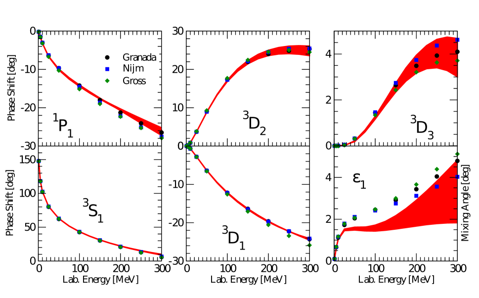
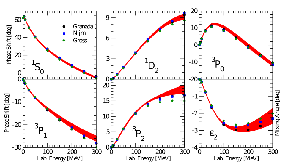
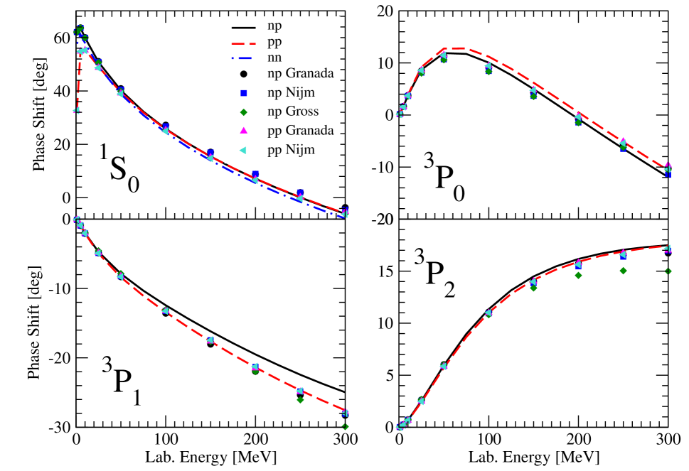
The S-wave, P-wave, and D-wave phase shits for $np$ (in $T=0$ and $T=1$) and $pp$ are displayed in Figs. 24 up to 300 MeV lab energies. The phases calculated with the full models a, b, and c including strong and electromagnetic interactions are represented by the band. The $np$ phases are relative to spherical Bessel functions, while the $pp$ phases are with respect to electromagnetic functions (see Appendix D). The cutoff sensitivity, as represented by the width of the shaded band, is very weak for $pp$, and generally remains modest for $np$, except for the $T=0$ 3D3 phase and $\epsilon_{1}$ mixing angle, particularly for energies larger than 150 MeV. The calculated phases are compared to those obtained in partial-wave analyses (PWA’s) by the Nijmegen Stoks93 ; Stoks94 , Granada Navarro13 , and Gross-Stadler Gross08 groups. Note that the recent Gross and Stadler’s PWA was limited to $np$ data only. We also should point out that, since the Nijmegen’s PWA of the early nineties which was based on about 1780 $pp$ and 2514 $np$ data in the lab energy range 0–350 MeV, the $NN$ elastic scattering database has increased very significantly. Indeed, in the same energy range the 2013 Granada database contains a total of 2972 $pp$ and 4737 $np$ data. Especially for the higher partial waves in the $np$ sector and at the larger energies there are appreciable differences between these various PWA’s. It is also interesting to observe that these differences are most significant for the $T=0$ 3D3 phase and $\epsilon_{1}$ mixing angle, and therefore correlate with the cutoff sensitivity displayed in these cases by models a, b, and c.

Refer to caption
Figure 2: (Color online) S-wave, P-wave, and D-wave phase shifts in the $np$ $T$=0 channel, obtained in the Nijmegen Stoks93 ; Stoks94 , Gross and Stadler Gross08 , and Navarro Pérez et al. Navarro13 partial-wave analyses, are compared to those of models a, b, and c, indicated by the band. For the mixing angle $\epsilon_{1}$ (phase shift 3D3) the lower limit of the band corresponds to model a (model b) and the upper limit to model c (model c).

The low-energy scattering parameters are listed in Table 5, where they are compared to experimental results. The singlet and triplet $np$, and singlet $pp$ and $nn$, scattering lengths are calculated with and without the inclusion of electromagnetic interactions. Without the latter, the effective range function is simply given by $F(k^{2})=k\,\cot\delta=-1/a+r\,k^{2}/2$ up to terms linear in $k^{2}$. In the presence of electromagnetic interactions, a more complicated effective range function must be used; it is reported in Appendix D, along with the relevant references. The latest determinations of the empirical values for the singlet scattering lengths and effective ranges, obtained by retaining only strong interactions (hence the superscript N), are Miller90 ; Machleidt01 ; Gonzalez06 ; Chen08 (as reported in Ref. Entem11 ):

${}^{1}a^{\rm N}_{pp}$ $\displaystyle=$ $\displaystyle-17.3\pm 0.4\,\,{\rm fm}\ ,\qquad^{1}r^{\rm N}_{pp}=2.85\pm 0.04\,\,{\rm fm}\ ,$ (31)
${}^{1}a^{\rm N}_{np}$ $\displaystyle=$ $\displaystyle-23.74\pm 0.02\,\,{\rm fm}\ ,\qquad^{1}r^{\rm N}_{np}=2.77\pm 0.05\,\,{\rm fm}\ ,$ (32)
${}^{1}a^{\rm N}_{nn}$ $\displaystyle=$ $\displaystyle-18.95\pm 0.4\,\,{\rm fm}\ ,\qquad^{1}r^{\rm N}_{nn}=2.75\pm 0.11\,\,{\rm fm}\ ,$ (33)

which imply that charge symmetry and charge independence are broken respectively by

$$\Delta a_{\rm CSB}=a_{pp}^{\rm N}-a_{nn}^{\rm N}=1.65\pm 0.60\,\,{\rm fm}\ ,\qquad\Delta r_{\rm CSB}=r_{pp}^{\rm N}-r_{nn}^{\rm N}=0.10\pm 0.12\,\,{\rm fm}\ ,$$ (34)

and

$$\Delta a_{\rm CIB}=(a_{pp}^{\rm N}+a_{nn}^{\rm N})/2-a_{np}^{\rm N}=5.6\pm 0.6\,\,{\rm fm}\ ,\qquad\Delta r_{\rm CIB}=(r_{pp}^{\rm N}+r_{nn}^{\rm N})/2-r_{np}^{\rm N}=0.03\pm 0.13\,\,{\rm fm}\ .$$ (35)

The more significant values for $\Delta a_{\rm CSB}$ and $\Delta a_{\rm CIB}$ can be compared to those inferred from Table 5: $(\Delta a_{\rm CSB},\Delta a_{\rm CIB})=(2.13,\,5.11)$ fm for model a, (2.34, 5.12) fm for model b, and (1.90, 5.08) fm for model c.

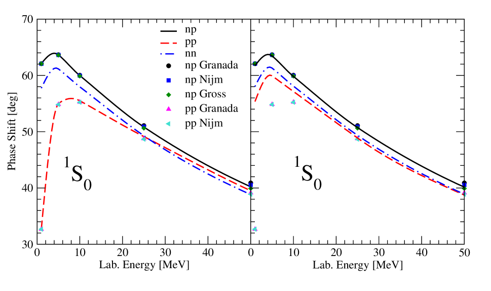
In the left upper panel of Fig. 5 we show the 1S0 phase shifts for $pp$, $np$ and $nn$ calculated with and without the inclusion of electromagnetic interactions (only model b is considered). There is excellent agreement between these phases and those obtained in the the Granada, Gross and Stadler, and Nijmegen PWA’s, when electromagnetic effects are fully accounted for. Particularly at low energies (see Fig. 6), the latter provide most of the splitting between the $pp$ and $np$ phases, with remaining differences originating from isospin symmetry breaking due to the OPE term in $v^{\rm L}_{12}$ and the central terms in $v^{\rm S,CD}_{12}$, proportional to the LEC’s $C_{i}^{\rm IT}$ and $C_{i}^{\rm IV}$ with $i=0$–2. In the absence of electromagnetic interactions, the splitting between the $pp$ and $nn$ 1S0 phases is induced by the charge-symmetry breaking terms of $v^{\rm S,CD}_{12}$ proportional to the LEC’s $C_{i}^{\rm IV}$ with $i=0$–2; it is smaller than that between $pp$ and $np$ 1S0 phases.

The effects of isospin symmetry breaking are also seen in the $pp$ and $np$ 3PJ phases with $J=0,1,2$ in the upper right and lower panels of Fig. 5, especially at the higher energies. The calculated phases, which correspond again to model b, include electromagnetic effects, but the latter are negligible beyond 100 MeV. The splitting between the $pp$ and $np$ 3PJ phases is mostly due to the isotensor and isovector terms of $v^{\rm S,CD}_{12}$, in particular those proportional to the LEC’s $C_{i}^{IV}$ and $C_{i}^{IT}$ with $i=3$ and 4 associated respectively with the tensor and spin-orbit components of $v^{\rm S,CD}_{12}$—we have already remarked on the unnaturally large values obtained for $C_{4}^{IV}$ and $C_{4}^{IT}$ in the fits. There is no evidence on the basis of the Granada and Nijmegen PWA’s for such a large splitting, and so the latter is likely to be an artifact of the parametrization adopted for $v^{\rm S,CD}_{12}$.

Refer to caption
Figure 3: (Color online) Same as in Fig. 2, but for the S-wave, P-wave, and D-wave phase shifts in the $np$ $T$=1 channel. For the mixing angle $\epsilon_{2}$ the lower limit of the band corresponds to model c and the upper limit to model b.
Refer to caption
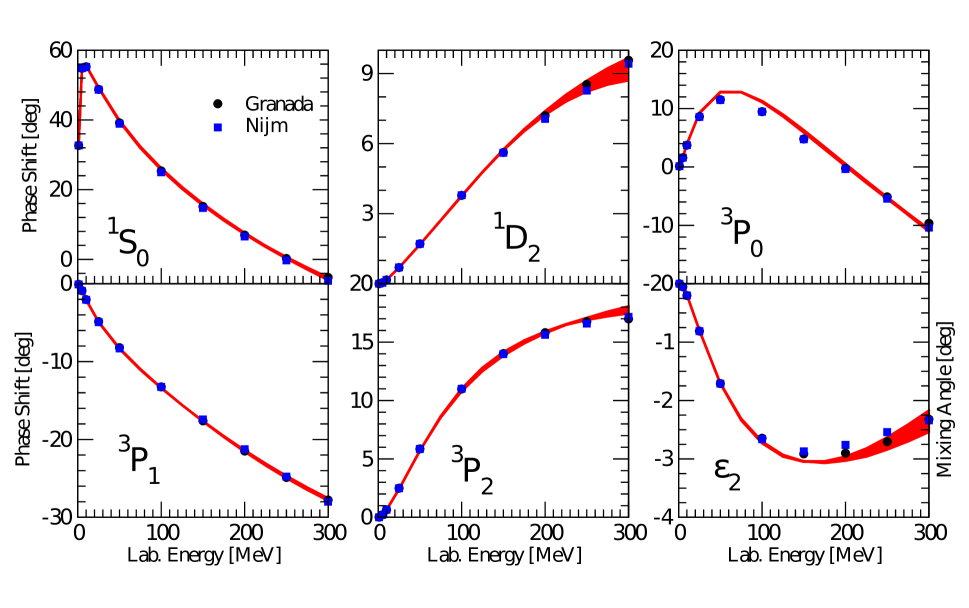
Figure 4: (Color online) S-wave, P-wave, and D-wave phase shifts in the $pp$ $T$=1 channel, obtained in the Nijmegen and Navarro Pérez et al. partial-wave analyses, are compared to those of models a, b, and c, indicated by the band.
Table 5: The singlet and triplet $np$, and singlet $pp$ and $nn$, scattering lengths and effective ranges corresponding to the three potential models with $(R_{\rm L},R_{\rm S})$=(1.2,0.8) fm (model a), (1.0,0.7) fm (model b), and (0.8,0.6) fm (model c).
Experiment $v_{12}^{a}$ w/o $v_{12}^{\rm EM}$ $v_{12}^{b}$ w/o $v_{12}^{\rm EM}$ $v_{12}^{c}$ w/o $v_{12}^{\rm EM}$
${}^{1}a_{pp}$ $-7.8063(26)$ $-7.766$ $-17.014$ $-7.766$ $-16.956$ $-7.763$ $-17.137$
$-7.8016(29)$
${}^{1}r_{pp}$ $2.794(14)$ $2.742$ $2.818$ $2.743$ $2.820$ $2.730$ $2.802$
$2.773(14)$
${}^{1}a_{nn}$ $-18.90(40)$ $-18.867$ $-19.148$ $-19.025$ $-19.301$ $-18.719$ $-19.039$
${}^{1}r_{nn}$ $2.75(11)$ $2.831$ $2.827$ $2.799$ $2.795$ $2.738$ $2.732$
${}^{1}a_{np}$ $-23.740(20)$ $-23.752$ $-23.196$ $-23.755$ $-23.248$ $-23.745$ $-23.167$
${}^{1}r_{np}$ $2.77(5)$ $2.665$ $2.670$ $2.672$ $2.677$ $2.638$ $2.644$
${}^{3}a_{np}$ $5.419(7)$ $5.408$ $5.391$ $5.404$ $5.389$ $5.412$ $5.396$
${}^{3}r_{np}$ $1.753(8)$ $1.741$ $1.740$ $1.737$ $1.734$ $1.740$ $1.745$
Refer to caption
Figure 5: (Color online) The $pp$, $np$, and $nn$ 1S0 and the $pp$ and $np$ 3P0, 3P1, and 3P2 phase shifts obtained with potential model b, including the full electromagnetic component.
Refer to caption
Figure 6: (Color online) The $pp$, $np$, and $nn$ 1S0 up to lab energy of 50 MeV including (panel left) and ignoring (panel right) the full electromagnetic component of potential model b.

The static deuteron properties are shown in Table 6 and compared to experimental values Vandl82 ; Ericson83 ; Rodning90 ; Huber98 ; Bishop79 . The binding energy Edsubscript𝐸𝑑E_{d} is fitted exactly and includes the contributions (about 20 keV) of electromagnetic interactions, among which the largest is that due to the magnetic moment term. The asymptotic S-state normalization, ASsubscript𝐴SA_{\rm S}, and the D/S ratio, η𝜂\eta, are both 2similar-toabsent2\sim 2 standard deviations from experiment for all models considered. The deuteron (matter) radius, rdsubscript𝑟𝑑r_{d}, is exactly reproduced with model b, but is under-predicted (over-predicted) by about 1.4% (0.7%) with model a (model c). It is should be noted that this observable has negligible contributions due to two-body electromagnetic operators Piarulli13 . The magnetic moment, μdsubscript𝜇𝑑\mu_{d}, and quadrupole moment, Qdsubscript𝑄𝑑Q_{d}, experimental values are underestimated by all three models, but these observables are known to have significant corrections from (isoscalar) two-body terms in nuclear electromagnetic charge and current Piarulli13 . Their inclusion would bring the calculated values considerably closer to, if not in agreement with, experiment. 
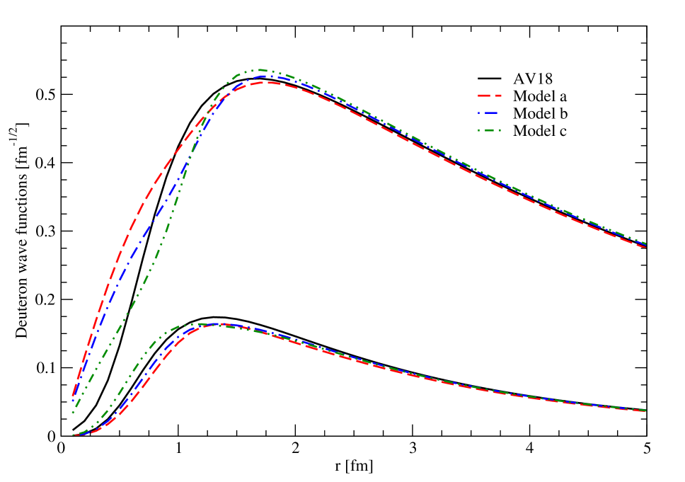
Finally, the S- and D-wave components of the deuteron wave function are displayed in Fig. 7, where they are compared to those of the Argonne v18subscript𝑣18v_{18} (AV18) model. There is significant cutoff dependence as (RL,RS)subscript𝑅Lsubscript𝑅S(R_{\rm L},R_{\rm S}) are reduced from the values (1.2, 0.8) fm of model a down to (0.8, 0.6) fm of model c. For r1less-than-or-similar-to𝑟1r\lesssim 1 fm, the S-wave becomes smaller (is pushed out), while the D-wave becomes larger (is pushed in) in going from model a to model c. The D-state percentage increases correspondingly (see Table 6).

We note in closing that in Appendix E we provide figures of the various components of potential models a, b, and c (their charge-independent parts only) as well as tables of numerical values for the $pp$ and $np$ S, P, D, F, and G phase shifts obtained with model b.

Table 6: Same as in Table 5 but for the deuteron static properties; experimental values are form Refs. Vandl82 ; Ericson83 ; Rodning90 ; Huber98 ; Bishop79 .
Experiment $v_{12}^{\rm a}$ $v_{12}^{\rm b}$ $v_{12}^{\rm c}$
$E_{d}$ (MeV) 2.224575(9) 2.224575 2.224574 2.224575
$A_{\rm S}$(fm-1/2) 0.8781(44) 0.8777 0.8904 0.8964
$\eta$ 0.0256(4) 0.0245 0.0248 0.0246
$r_{d}$ (fm) 1.97535(85) 1.948 1.975 1.989
$\mu_{d}$ ($\mu_{0}$) 0.857406(1) 0.852 0.850 0.848
$Q_{d}$ (fm2) 0.2859(3) 0.257 0.268 0.269
$P_{d}$ (%) 4.94 5.29 5.55
Refer to caption
Figure 7: (Color online) The $S$-wave and $D$-wave components of the deuteron wave function corresponding to models a (dashed lines), b (dotted-dashed lines) and c (dotted-dashed-dotted lines) are compared with those corresponding to the AV18 (solid lines).

V Conclusions

In the present study, we have constructed a coordinate-space nucleon-nucleon potential with an electromagnetic interaction component including first and second order Coulomb, Darwin-Foldy, vacuum polarization, and magnetic moment terms, and a strong interaction component characterized by long- and short-range parts. The long-range part includes OPE and TPE terms up to N2LO, derived in the static limit from leading and sub-leading $\pi N$ and $\pi N\Delta$ chiral Lagrangians. Its strength is fully determined by the nucleon and nucleon-to-$\Delta$ axial coupling constants $g_{A}$ and $h_{A}$, the pion decay amplitude $F_{\pi}$, and the sub-leading LEC’s $c_{1}$, $c_{2}$, $c_{3}$, $c_{4}$, and $b_{3}+b_{8}$, constrained by reproducing $\pi N$ scattering data (the values adopted for all these couplings are listed in Table 1). In coordinate space, this long-range part is represented by charge-independent central, spin, and tensor components without and with the isospin dependence ${\bm{\tau}}_{1}\cdot{\bm{\tau}}_{2}$ (the so-called $v_{6}$ operator structure), and by charge-dependence-breaking central and tensor components induced by OPE and proportional to the isotensor operator $T_{12}$.

The short-range part is described by charge-independent contact interactions specified by a total of 24 LEC’s (2 at LO, 7 at NLO, and 15 at N3LO) and by charge-dependent ones characterized by 10 LEC’s (2 at LO and 8 at NLO), 5 of which multiply charge-symmetry breaking terms proportional to $\tau_{1z}+\tau_{2z}$ and the remaining 5 multiply charge-dependence breaking terms proportional to $T_{12}$. In the NLO and N3LO contact interactions, Fierz transformations have been used in order to rearrange terms that in coordinate space would otherwise lead to powers of ${\bf p}$—the relative momentum operator—higher than two. The resulting charge-independent (coordinate-space) potential contains, in addition to the $v_{6}$ operator structure, spin-orbit, ${\bf L}^{2}$, quadratic-spin-orbit, and ${\bf p}^{2}$ components, while the charge-dependent one retains central, tensor, and spin-orbit components.

The 34 LEC’s in the short-range potential have been constrained by fitting 5291 $pp$ and $np$ scattering data (including normalizations) up to 300 MeV lab energies, as assembled in the Granada database, and the $pp$, $np$, and $nn$ scattering lengths, and the deuteron binding energy. The global $\chi^{2}(pp+np)$/datum is 1.33 for the three different models we have investigated, each specified by a pair of (coordinate-space) cutoffs, respectively, $R_{\rm L}$ and $R_{\rm S}$ for the long- and short-range parts: $(R_{\rm L},R_{\rm S})=(1.2,0.8)$ fm for model a, $(1.0,0.7)$ fm for model b, and $(0.8,0.6)$ fm for model c. These cutoffs are close to the $1/(2\,m_{\pi})\sim 0.7$ fm TPE range. The values of the LEC’s corresponding to the three models are given in Table 4. They are generally of natural size, but for a few exceptions, most notably the LEC’s $C_{4}^{\rm IV}$ and $C_{4}^{\rm IT}$ multiplying the charge-dependent spin-orbit terms, which lead to relatively large splitting between the $pp$ and $np$ 3P0 and 3P1 phase shifts—a splitting that is not consistent with that obtained in both the Nijmegen and Granada PWA’s. It should also be noted that the degree of unnaturalness increases as the short-distance cutoffs are reduced.

Our results suggest that discrepancies between the phases calculated here and those from available PWA’s in some of the partial waves, such as the $\epsilon_{1}$ mixing angle, could hardly be resolved by carrying out the database selection using the present interaction. We should also note that the renowned Entem and Machleidt N3LO fit up to $E_{\rm lab}=290$ MeV provides a $\chi^{2}$/datum of 1.1 for 2402 $np$ data and 1.5 for 2057 $pp$, and hence a global $\chi^{2}$/datum of 1.3. In our case, we describe 2161 (2764) scattering data and 148 (218) normalizations for $pp$ ($np$), which means that the average contribution to the $\chi^{2}$ from each additional datum is homogeneous and of order one out of about 800 extra data. So, our fit is as good as the one of Entem and Machleidt with these additional data.

According to our findings the largest uncertainty in the chiral theory when fitting up to a maximum lab energy of 300 MeV is provided by the cutoff dependence. Under these circumstances it makes little sense to analyze further uncertainties, but it is nonetheless surprising that precisely the model implementing many QCD motivated theoretical constraints should end up magnifying the uncertainty to a larger extent than the spread historically found in all so far successful PWA’s to $pp$ and $np$ scattering data. On the other hand, the reliability of the long distance chiral interaction does not depend on how the short distance unknown interaction is organized. This has been proven by the first chiral potential fits by the Nijmegen group from their $pp$ Rentmeester:1999vw and $np+pp$ Rentmeester:2003mf analyses and more recently verified with increased statistics by the Granada group Perez:2013oba . This leaves open the possibility that better fits than those found here should be possible by properly altering the short distance structure. This point has recently been discussed in Ref. Perez:2014bua .

Of course, this cutoff uncertainty could be greatly reduced if the fitting energy range were to be lowered so as to ensure that differences between fitted data and fitting theory fulfill the normality requirement and, at the same time, statistical uncertainties remain at the same level as cutoff uncertainties. Following the recent suggestion Perez:2014bua , we find that this happens with the current form of the potential when $E_{\rm lab}\leq 125$ MeV. In a companion paper we will analyze the statistical properties of the present fit and how there is a trade-off of different uncertainty sources.

We conclude by observing that, apart from the ${\bf p}^{2}$-dependent terms, the potential constructed here has the same operator structure of the AV18, and is of slightly better quality than the AV18 (the AV18 global $\chi^{2}(pp+np)$/datum on the same database up to 300 MeV lab energies is 1.46). It should be fairly straightforward to incorporate it in the few-nucleon calculations based on hyperspherical-harmonics expansion techniques favored by the Pisa group Kievsky08 , or in the quantum Monte Carlo ones preferred by the ANL/ASU/JLab/LANL collaboration Carlson2014 . The Fortran computer program generating the potential will be made available upon request.

Acknowledgements.
We like to thank J. Sarich and S.M. Wild in the Mathematics and Computer Science Division at Argonne National Laboratory for advise on the implementation of POUNDerS in the $\chi^{2}$-minimization programs. Conversations with F. Gross, J.W. Van Orden, and R.B. Wiringa at various stages of this project are gratefully acknowledged. Finally, we also like to thank D. Lonardoni and A. Lovato for help on the parallelization of the minimization programs. The work of R.S. is supported by the U.S. Department of Energy, Office of Nuclear Science, under contract DE-AC05-06OR23177. The work of R.N.P., J.E.A., and E.R.A. is supported by the Spanish DGI (grant FIS2011-24149) and Junta de Andalucía (grant FQM225). R.N.P. is also supported by a Mexican CONACYT grant. The calculations were made possible by grants of computing time from the National Energy Research Supercomputer Center (NERSC).

Appendix A Coordinate-space representation of the potential $v^{\rm L}_{12}$

The LO (OPE) terms corresponding to diagram (a) in Fig. 1 are given by

$\displaystyle v^{\rm LO}_{\sigma\tau}(r)$ $\displaystyle=$ $\displaystyle\frac{Y_{0}(r)+2\,Y_{+}(r)}{3}\ ,$ (36)
$\displaystyle v^{\rm LO}_{t\tau}(r)$ $\displaystyle=$ $\displaystyle\frac{T_{0}(r)+2\,T_{+}(r)}{3}\ ,$ (37)

where

$\displaystyle Y_{\alpha}(r)$ $\displaystyle=$ $\displaystyle\frac{g_{A}^{2}}{12\,\pi}\,\frac{m^{3}_{\pi_{\alpha}}}{F_{\pi}^{2}}\,\frac{e^{-x_{\alpha}}}{x_{\alpha}}\ ,$ (38)
$\displaystyle T_{\alpha}(r)$ $\displaystyle=$ $\displaystyle Y_{\alpha}(r)\left(1+\frac{3}{x_{\alpha}}+\frac{3}{x^{2}_{\alpha}}\right)\ ,$ (39)

and $x_{\alpha}=m_{\pi_{\alpha}}r$. The NLO terms corresponding to diagrams (b)-(d) read Kaiser:1997mw

$\displaystyle v^{\rm NLO}_{\tau}(r;\not{\Delta})$ $\displaystyle=$ $\displaystyle\frac{1}{8\pi^{3}r^{4}}\frac{m_{\pi}}{F_{\pi}^{4}}\,\bigg{[}\,x\left[1+10g_{A}^{2}-g_{A}^{4}(23+4x^{2})\right]K_{0}(2x)$ (40)
$\displaystyle+\left[1+2g_{A}^{2}(5+2x^{2})-g_{A}^{4}(23+12x^{2})\right]K_{1}(2x)\bigg{]}\ ,$
$\displaystyle v^{\rm NLO}_{\sigma}(r;\not{\Delta})$ $\displaystyle=$ $\displaystyle\frac{1}{2\pi^{3}r^{4}}\frac{g_{A}^{4}}{F_{\pi}^{4}}\,m_{\pi}\bigg{[}3x\,K_{0}(2x)+(3+2x^{2})K_{1}(2x)\bigg{]}\ ,$ (41)
$\displaystyle v^{\rm NLO}_{t}(r;\not{\Delta})$ $\displaystyle=$ $\displaystyle-\frac{1}{8\pi^{3}r^{4}}\frac{g_{A}^{4}}{F_{\pi}^{4}}\,m_{\pi}\bigg{[}12x\,K_{0}(2x)+(15+4x^{2})K_{1}(2x)\bigg{]}\ ,$ (42)

where $x=m_{\pi}r$ ($m_{\pi}$ is the average pion mass) and $K_{n}$ are modified Bessel functions of the second kind. The NLO terms corresponding to diagrams (e)-(f) with a single $\Delta$ intermediate state are given by

$\displaystyle v^{\rm NLO}_{c}(r;\Delta)$ $\displaystyle=$ $\displaystyle-\frac{1}{6\pi^{2}r^{5}\,y}\frac{g_{A}^{2}h_{A}^{2}}{F_{\pi}^{4}}e^{-2x}\left(6+12x+10x^{2}+4x^{3}+x^{4}\right)\ ,$ (43)
$\displaystyle v^{\rm NLO}_{\tau}(r;\Delta)$ $\displaystyle=$ $\displaystyle-\frac{1}{216\pi^{3}r^{5}}\frac{h_{A}^{2}}{F_{\pi}^{4}}\Bigg{[}\int_{0}^{\infty}d\mu\frac{\mu^{2}}{\sqrt{\mu^{2}+4x^{2}}}e^{-\sqrt{\mu^{2}+4x^{2}}}(12x^{2}+5\mu^{2}+12y^{2})$ (44)
$\displaystyle-12y\int_{0}^{\infty}d\mu\frac{\mu}{\sqrt{\mu^{2}+4x^{2}}}e^{-\sqrt{\mu^{2}+4x^{2}}}(2x^{2}+\mu^{2}+2y^{2})\arctan{\frac{\mu}{2y}}\Bigg{]}$
$\displaystyle-\frac{1}{216\pi^{3}r^{5}}\frac{g_{A}^{2}h_{A}^{2}}{F_{\pi}^{4}}\Bigg{[}-\int_{0}^{\infty}d\mu\frac{\mu^{2}}{\sqrt{\mu^{2}+4x^{2}}}e^{-\sqrt{\mu^{2}+4x^{2}}}(24x^{2}+11\mu^{2}+12y^{2})$
$\displaystyle+\frac{6}{y}\int_{0}^{\infty}d\mu\frac{\mu}{\sqrt{\mu^{2}+4x^{2}}}e^{-\sqrt{\mu^{2}+4x^{2}}}(2x^{2}+\mu^{2}+2y^{2})^{2}\arctan{\frac{\mu}{2y}}\Bigg{]}\ ,$
$\displaystyle v^{\rm NLO}_{\sigma}(r;\Delta)$ $\displaystyle=$ $\displaystyle-\frac{1}{72\pi^{3}r^{5}}\frac{g_{A}^{2}h_{A}^{2}}{F_{\pi}^{4}}\Bigg{[}2\,\int_{0}^{\infty}d\mu\frac{\mu^{2}}{\sqrt{\mu^{2}+4x^{2}}}e^{-\sqrt{\mu^{2}+4x^{2}}}(\mu^{2}+4x^{2})$ (45)
$\displaystyle-\frac{1}{y}\int_{0}^{\infty}d\mu\frac{\mu}{\sqrt{\mu^{2}+4x^{2}}}e^{-\sqrt{\mu^{2}+4x^{2}}}(\mu^{2}+4x^{2})(\mu^{2}+4y^{2})\arctan{\frac{\mu}{2y}}\Bigg{]}\ ,$
$\displaystyle v^{\rm NLO}_{\sigma\tau}(r;\Delta)$ $\displaystyle=$ $\displaystyle\frac{1}{54\pi^{2}r^{5}\,y}\frac{g_{A}^{2}h_{A}^{2}}{F_{\pi}^{4}}e^{-2x}\left(1+x\right)\left(3+3x+x^{2}\right)\ ,$ (46)
$\displaystyle v^{\rm NLO}_{t}(r;\Delta)$ $\displaystyle=$ $\displaystyle\frac{1}{144\pi^{3}r^{5}}\frac{g_{A}^{2}h_{A}^{2}}{F_{\pi}^{4}}\Bigg{[}2\,\int_{0}^{\infty}d\mu\frac{\mu^{2}}{\sqrt{\mu^{2}+4x^{2}}}e^{-\sqrt{\mu^{2}+4x^{2}}}(3+3\sqrt{\mu^{2}+4x^{2}}+\mu^{2}+4x^{2})$ (47)
$\displaystyle-\frac{1}{y}\int_{0}^{\infty}d\mu\frac{\mu}{\sqrt{\mu^{2}+4x^{2}}}e^{-\sqrt{\mu^{2}+4x^{2}}}(\mu^{2}+4y^{2})(3+3\sqrt{\mu^{2}+4x^{2}}+\mu^{2}+4x^{2})\arctan{\frac{\mu}{2y}}\Bigg{]}\ ,$
$\displaystyle v^{\rm NLO}_{t\tau}(r;\Delta)$ $\displaystyle=$ $\displaystyle-\frac{1}{54\pi^{2}r^{5}\,y}\frac{g_{A}^{2}h_{A}^{2}}{F_{\pi}^{4}}e^{-2x}\left(1+x\right)\left(3+3x+2x^{2}\right)\ ,$ (48)

where $y=\Delta Mr$ ($\Delta M$ is the $\Delta$-nucleon mass difference) and the parametric integral over $\mu$ is carried out numerically. The NLO terms corresponding to diagram (g) with $2\,\Delta$ intermediate states are

$\displaystyle v^{\rm NLO}_{c}(r;2\Delta)$ $\displaystyle=$ $\displaystyle-\frac{1}{108\pi^{3}r^{5}}\frac{h_{A}^{4}}{F_{\pi}^{4}}\Bigg{[}\int_{0}^{\infty}d\mu\frac{\mu^{2}}{\sqrt{\mu^{2}+4x^{2}}}e^{-\sqrt{\mu^{2}+4x^{2}}}\left[4y^{2}+2\frac{(2x^{2}+\mu^{2}+2y^{2})^{2}}{(\mu^{2}+4y^{2})}\right]$ (49)
$\displaystyle+\frac{1}{y}\int_{0}^{\infty}d\mu\frac{\mu}{\sqrt{\mu^{2}+4x^{2}}}e^{-\sqrt{\mu^{2}+4x^{2}}}(2x^{2}+\mu^{2}+2y^{2})(2x^{2}+\mu^{2}-6y^{2})\arctan{\frac{\mu}{2y}}\Bigg{]}\ ,$
$\displaystyle v^{\rm NLO}_{\tau}(r;2\Delta)$ $\displaystyle=$ $\displaystyle-\frac{1}{1944\pi^{3}r^{5}}\frac{h_{A}^{4}}{F_{\pi}^{4}}\Bigg{[}\int_{0}^{\infty}d\mu\frac{\mu^{2}}{\sqrt{\mu^{2}+4x^{2}}}e^{-\sqrt{\mu^{2}+4x^{2}}}\left[(24x^{2}+11\mu^{2}+24y^{2})+6\frac{(2x^{2}+\mu^{2}+2y^{2})^{2}}{(\mu^{2}+4y^{2})}\right]$ (50)
$\displaystyle-\frac{3}{y}\int_{0}^{\infty}d\mu\frac{\mu}{\sqrt{\mu^{2}+4x^{2}}}e^{-\sqrt{\mu^{2}+4x^{2}}}(2x^{2}+\mu^{2}+2y^{2})(2x^{2}+\mu^{2}+10y^{2})\arctan{\frac{\mu}{2y}}\Bigg{]}\ ,$
$\displaystyle v^{\rm NLO}_{\sigma}(r;2\Delta)$ $\displaystyle=$ $\displaystyle-\frac{1}{1296\pi^{3}r^{5}}\frac{h_{A}^{4}}{F_{\pi}^{4}}\Bigg{[}-6\int_{0}^{\infty}d\mu\frac{\mu^{2}}{\sqrt{\mu^{2}+4x^{2}}}e^{-\sqrt{\mu^{2}+4x^{2}}}(\mu^{2}+4x^{2})$ (51)
$\displaystyle+\frac{1}{y}\int_{0}^{\infty}d\mu\frac{\mu}{\sqrt{\mu^{2}+4x^{2}}}e^{-\sqrt{\mu^{2}+4x^{2}}}(\mu^{2}+4x^{2})(\mu^{2}+12y^{2})\arctan{\frac{\mu}{2y}}\Bigg{]}\ ,$
$\displaystyle v^{\rm NLO}_{\sigma\tau}(r;2\Delta)$ $\displaystyle=$ $\displaystyle-\frac{1}{7776\pi^{3}r^{5}}\frac{h_{A}^{4}}{F_{\pi}^{4}}\Bigg{[}-2\int_{0}^{\infty}d\mu\frac{\mu^{2}}{\sqrt{\mu^{2}+4x^{2}}}e^{-\sqrt{\mu^{2}+4x^{2}}}(\mu^{2}+4x^{2})$ (52)
$\displaystyle+\frac{1}{y}\int_{0}^{\infty}d\mu\frac{\mu}{\sqrt{\mu^{2}+4x^{2}}}e^{-\sqrt{\mu^{2}+4x^{2}}}(\mu^{2}+4x^{2})(-\mu^{2}+4y^{2})\arctan{\frac{\mu}{2y}}\Bigg{]}\ ,$
$\displaystyle v^{\rm NLO}_{t}(r;2\Delta)$ $\displaystyle=$ $\displaystyle\frac{1}{2592\pi^{3}r^{5}}\frac{h_{A}^{4}}{F_{\pi}^{4}}\Bigg{[}-6\int_{0}^{\infty}d\mu\frac{\mu^{2}}{\sqrt{\mu^{2}+4x^{2}}}e^{-\sqrt{\mu^{2}+4x^{2}}}(3+3\sqrt{\mu^{2}+4x^{2}}+\mu^{2}+4x^{2})$ (53)
$\displaystyle+\frac{1}{y}\int_{0}^{\infty}d\mu\frac{\mu}{\sqrt{\mu^{2}+4x^{2}}}e^{-\sqrt{\mu^{2}+4x^{2}}}(3+3\sqrt{\mu^{2}+4x^{2}}+\mu^{2}+4x^{2})(\mu^{2}+12y^{2})\arctan{\frac{\mu}{2y}}\Bigg{]}\ ,$
$\displaystyle v^{\rm NLO}_{t\tau}(r;2\Delta)$ $\displaystyle=$ $\displaystyle\frac{1}{15552\pi^{3}r^{5}}\frac{h_{A}^{4}}{F_{\pi}^{4}}\Bigg{[}-2\int_{0}^{\infty}d\mu\frac{\mu^{2}}{\sqrt{\mu^{2}+4x^{2}}}e^{-\sqrt{\mu^{2}+4x^{2}}}(3+3\sqrt{\mu^{2}+4x^{2}}+\mu^{2}+4x^{2})$ (54)
$\displaystyle+\frac{1}{y}\int_{0}^{\infty}d\mu\frac{\mu}{\sqrt{\mu^{2}+4x^{2}}}e^{-\sqrt{\mu^{2}+4x^{2}}}(3+3\sqrt{\mu^{2}+4x^{2}}+\mu^{2}+4x^{2})(-\mu^{2}+4y^{2})\arctan{\frac{\mu}{2y}}\Bigg{]}\ .$

Moving on to the loop corrections at N2LO, the terms corresponding to diagrams (h)-(k) are given by

$\displaystyle v^{\rm N2LO}_{c}(r;\not{\Delta})$ $\displaystyle=$ $\displaystyle\frac{3}{2\,\pi^{2}r^{6}}\frac{g_{A}^{2}}{F_{\pi}^{4}}e^{-2x}\left[2c_{1}x^{2}(1+x)^{2}+c_{3}(6+12x+10x^{2}+4x^{3}+x^{4})\right]\ ,$ (55)
$\displaystyle v^{\rm N2LO}_{\sigma\tau}(r;\not{\Delta})$ $\displaystyle=$ $\displaystyle\frac{1}{3\,\pi^{2}r^{6}}\frac{g_{A}^{2}}{F_{\pi}^{4}}c_{4}e^{-2x}\left(1+x\right)\left(3+3x+2x^{2}\right)\ ,$ (56)
$\displaystyle v^{\rm N2LO}_{t\tau}(r;\not{\Delta})$ $\displaystyle=$ $\displaystyle-\frac{1}{3\,\pi^{2}r^{6}}\frac{g_{A}^{2}}{F_{\pi}^{4}}c_{4}e^{-2x}\left(1+x\right)\left(3+3x+x^{2}\right)\ ,$ (57)

while those corresponding to diagrams (l)-(o) are given by

$\displaystyle v^{\rm N2LO}_{c}(r;\Delta)$ $\displaystyle=$ $\displaystyle\frac{1}{18\pi^{3}r^{6}}\frac{h_{A}^{2}\,y}{F_{\pi}^{4}}\Bigg{[}\int_{0}^{\infty}d\mu\frac{\mu^{2}}{\sqrt{\mu^{2}+4x^{2}}}e^{-\sqrt{\mu^{2}+4x^{2}}}[-24c_{1}x^{2}+c_{2}(5\mu^{2}+12x^{2}+12y^{2})-6c_{3}(\mu^{2}+2x^{2})]$ (58)
$\displaystyle+\frac{6}{y}\int_{0}^{\infty}\!\!d\mu\frac{\mu}{\sqrt{\mu^{2}+4x^{2}}}e^{-\sqrt{\mu^{2}+4x^{2}}}(\mu^{2}\!+\!2x^{2}\!+\!2y^{2})[4c_{1}x^{2}-2c_{2}y^{2}+c_{3}(\mu^{2}+2x^{2})]\,\arctan{\frac{\mu}{2y}}\Bigg{]}\ ,$
$\displaystyle v^{\rm N2LO}_{\tau}(r;\Delta)$ $\displaystyle=$ $\displaystyle-\frac{1}{54\pi^{3}r^{6}}\frac{(b_{3}+b_{8})\,h_{A}\,y}{F_{\pi}^{4}}\Bigg{[}+\int_{0}^{\infty}d\mu\frac{\mu^{2}}{\sqrt{\mu^{2}+4x^{2}}}e^{-\sqrt{\mu^{2}+4x^{2}}}(5\mu^{2}+12x^{2}+12y^{2})$ (59)
$\displaystyle-12\,y\int_{0}^{\infty}d\mu\frac{\mu}{\sqrt{\mu^{2}+4x^{2}}}e^{-\sqrt{\mu^{2}+4x^{2}}}(\mu^{2}+2x^{2}+2y^{2})\,\arctan{\frac{\mu}{2y}}\Bigg{]}$
$\displaystyle-\frac{1}{54\pi^{3}r^{6}}\frac{(b_{3}+b_{8})\,h_{A}\,g_{A}^{2}\,y}{F_{\pi}^{4}}\Bigg{[}-\int_{0}^{\infty}d\mu\frac{\mu^{2}}{\sqrt{\mu^{2}+4x^{2}}}e^{-\sqrt{\mu^{2}+4x^{2}}}(11\mu^{2}+24x^{2}+12y^{2})$
$\displaystyle+\frac{6}{y}\int_{0}^{\infty}d\mu\frac{\mu}{\sqrt{\mu^{2}+4x^{2}}}e^{-\sqrt{\mu^{2}+4x^{2}}}\left(\mu^{2}+2x^{2}+2y^{2}\right)^{2}\arctan{\frac{\mu}{2y}}\Bigg{]}\ ,$
$\displaystyle v^{\rm N2LO}_{\sigma}(r;\Delta)$ $\displaystyle=$ $\displaystyle-\frac{1}{18\pi^{3}r^{6}}\frac{(b_{3}+b_{8})\,h_{A}\,g_{A}^{2}\,y}{F_{\pi}^{4}}\Bigg{[}2\int_{0}^{\infty}d\mu\frac{\mu^{2}}{\sqrt{\mu^{2}+4x^{2}}}e^{-\sqrt{\mu^{2}+4x^{2}}}(\mu^{2}+4x^{2})$ (60)
$\displaystyle-\frac{1}{y}\int_{0}^{\infty}d\mu\frac{\mu}{\sqrt{\mu^{2}+4x^{2}}}e^{-\sqrt{\mu^{2}+4x^{2}}}(\mu^{2}+4x^{2})(\mu^{2}+4y^{2})\arctan{\frac{\mu}{2y}}\Bigg{]}\ ,$
$\displaystyle v^{\rm N2LO}_{\sigma\tau}(r;\Delta)$ $\displaystyle=$ $\displaystyle-\frac{1}{108\pi^{3}r^{6}}\frac{c_{4}\,h_{A}^{2}\,y}{F_{\pi}^{4}}\Bigg{[}2\,\int_{0}^{\infty}d\mu\frac{\mu^{2}}{\sqrt{\mu^{2}+4x^{2}}}e^{-\sqrt{\mu^{2}+4x^{2}}}(\mu^{2}+4x^{2})$ (61)
$\displaystyle-\frac{1}{y}\int_{0}^{\infty}d\mu\frac{\mu}{\sqrt{\mu^{2}+4x^{2}}}e^{-\sqrt{\mu^{2}+4x^{2}}}(\mu^{2}+4x^{2})(\mu^{2}+4y^{2})\,\arctan{\frac{\mu}{2y}}\Bigg{]}\ ,$
$\displaystyle v^{\rm N2LO}_{t}(r;\Delta)$ $\displaystyle=$ $\displaystyle\frac{1}{36\pi^{3}r^{6}}\frac{(b_{3}+b_{8})\,h_{A}\,g_{A}^{2}\,y}{F_{\pi}^{4}}\Bigg{[}2\int_{0}^{\infty}d\mu\frac{\mu^{2}}{\sqrt{\mu^{2}+4x^{2}}}e^{-\sqrt{\mu^{2}+4x^{2}}}(3+3\sqrt{\mu^{2}+4x^{2}}+\mu^{2}+4x^{2})$ (62)
$\displaystyle-\frac{1}{y}\int_{0}^{\infty}d\mu\frac{\mu}{\sqrt{\mu^{2}+4x^{2}}}e^{-\sqrt{\mu^{2}+4x^{2}}}(3+3\sqrt{\mu^{2}+4x^{2}}+\mu^{2}+4x^{2})(\mu^{2}+4y^{2})\arctan{\frac{\mu}{2y}}\Bigg{]}\ ,$
$\displaystyle v^{\rm N2LO}_{t\tau}(r;\Delta)$ $\displaystyle=$ $\displaystyle\frac{1}{216\pi^{3}r^{6}}\frac{c_{4}\,h_{A}^{2}\,y}{F_{\pi}^{4}}\Bigg{[}2\,\int_{0}^{\infty}d\mu\frac{\mu^{2}}{\sqrt{\mu^{2}+4x^{2}}}e^{-\sqrt{\mu^{2}+4x^{2}}}(3+3\sqrt{\mu^{2}+4x^{2}}+\mu^{2}+4x^{2})$ (63)
$\displaystyle-\frac{1}{y}\int_{0}^{\infty}d\mu\frac{\mu}{\sqrt{\mu^{2}+4x^{2}}}e^{-\sqrt{\mu^{2}+4x^{2}}}(3+3\sqrt{\mu^{2}+4x^{2}}+\mu^{2}+4x^{2})(\mu^{2}+4y^{2})\,\arctan{\frac{\mu}{2y}}\Bigg{]}\ .$

Lastly, the contributions corresponding to diagram (p) read

$\displaystyle v^{\rm N2LO}_{c}(r;2\Delta)$ $\displaystyle=$ $\displaystyle-\frac{2}{81\pi^{3}r^{6}}\frac{(b_{3}+b_{8})\,h_{A}^{3}\,y}{F_{\pi}^{4}}\Bigg{[}\int_{0}^{\infty}d\mu\frac{\mu^{2}}{\sqrt{\mu^{2}+4x^{2}}}e^{-\sqrt{\mu^{2}+4x^{2}}}[6\frac{(\mu^{2}+2x^{2}+2y^{2})^{2}}{\mu^{2}+4y^{2}}+11\mu^{2}+24x^{2}+12y^{2}]$ (64)
$\displaystyle-\frac{3}{y}\int_{0}^{\infty}d\mu\frac{\mu}{\sqrt{\mu^{2}+4x^{2}}}e^{-\sqrt{\mu^{2}+4x^{2}}}(\mu^{2}+2x^{2}+10y^{2})(\mu^{2}+2x^{2}+2y^{2})\arctan{\frac{\mu}{2y}}\Bigg{]}\ ,$
$\displaystyle v^{\rm N2LO}_{\tau}(r;2\Delta)$ $\displaystyle=$ $\displaystyle-\frac{1}{243\pi^{3}r^{6}}\frac{(b_{3}+b_{8})\,h_{A}^{3}\,y}{F_{\pi}^{4}}\Bigg{[}\int_{0}^{\infty}d\mu\frac{\mu^{2}}{\sqrt{\mu^{2}+4x^{2}}}e^{-\sqrt{\mu^{2}+4x^{2}}}[6\frac{(\mu^{2}+2x^{2}+2y^{2})^{2}}{\mu^{2}+4y^{2}}+11\mu^{2}+24x^{2}+12y^{2}]$ (65)
$\displaystyle-\frac{3}{y}\int_{0}^{\infty}d\mu\frac{\mu}{\sqrt{\mu^{2}+4x^{2}}}e^{-\sqrt{\mu^{2}+4x^{2}}}(\mu^{2}+2x^{2}+10y^{2})(\mu^{2}+2x^{2}+2y^{2})\arctan{\frac{\mu}{2y}}\Bigg{]}\ ,$
$\displaystyle v^{\rm N2LO}_{\sigma}(r;2\Delta)$ $\displaystyle=$ $\displaystyle-\frac{1}{162\pi^{3}r^{6}}\frac{(b_{3}+b_{8})\,h_{A}^{3}\,y}{F_{\pi}^{4}}\Bigg{[}-6\int_{0}^{\infty}d\mu\frac{\mu^{2}}{\sqrt{\mu^{2}+4x^{2}}}e^{-\sqrt{\mu^{2}+4x^{2}}}(\mu^{2}+4x^{2})$ (66)
$\displaystyle+\frac{1}{y}\int_{0}^{\infty}d\mu\frac{\mu}{\sqrt{\mu^{2}+4x^{2}}}e^{-\sqrt{\mu^{2}+4x^{2}}}(\mu^{2}+4x^{2})(\mu^{2}+12y^{2})\arctan{\frac{\mu}{2y}}\Bigg{]}\ ,$
$\displaystyle v^{\rm N2LO}_{\sigma\tau}(r;2\Delta)$ $\displaystyle=$ $\displaystyle-\frac{1}{972\pi^{3}r^{6}}\frac{(b_{3}+b_{8})\,h_{A}^{3}\,y}{F_{\pi}^{4}}\Bigg{[}-6\int_{0}^{\infty}d\mu\frac{\mu^{2}}{\sqrt{\mu^{2}+4x^{2}}}e^{-\sqrt{\mu^{2}+4x^{2}}}(\mu^{2}+4x^{2})$ (67)
$\displaystyle+\frac{1}{y}\int_{0}^{\infty}d\mu\frac{\mu}{\sqrt{\mu^{2}+4x^{2}}}e^{-\sqrt{\mu^{2}+4x^{2}}}(\mu^{2}+4x^{2})(\mu^{2}+12y^{2})\arctan{\frac{\mu}{2y}}\Bigg{]}\ ,$
$\displaystyle v^{\rm N2LO}_{t}(r;2\Delta)$ $\displaystyle=$ $\displaystyle\frac{1}{324\pi^{3}r^{6}}\frac{(b_{3}+b_{8})\,h_{A}^{3}\,y}{F_{\pi}^{4}}\Bigg{[}-6\int_{0}^{\infty}d\mu\frac{\mu^{2}}{\sqrt{\mu^{2}+4x^{2}}}e^{-\sqrt{\mu^{2}+4x^{2}}}(3+3\sqrt{\mu^{2}+4x^{2}}+\mu^{2}+4x^{2})$ (68)
$\displaystyle+\frac{1}{y}\int_{0}^{\infty}d\mu\frac{\mu}{\sqrt{\mu^{2}+4x^{2}}}e^{-\sqrt{\mu^{2}+4x^{2}}}(3+3\sqrt{\mu^{2}+4x^{2}}+\mu^{2}+4x^{2})(\mu^{2}+12y^{2})\arctan{\frac{\mu}{2y}}\Bigg{]}\ ,$
$\displaystyle v^{\rm N2LO}_{t\tau}(r;2\Delta)$ $\displaystyle=$ $\displaystyle\frac{1}{1944\pi^{3}r^{6}}\frac{(b_{3}+b_{8})\,h_{A}^{3}\,y}{F_{\pi}^{4}}\Bigg{[}-6\int_{0}^{\infty}d\mu\frac{\mu^{2}}{\sqrt{\mu^{2}+4x^{2}}}e^{-\sqrt{\mu^{2}+4x^{2}}}(3+3\sqrt{\mu^{2}+4x^{2}}+\mu^{2}+4x^{2})$ (69)
$\displaystyle+\frac{1}{y}\int_{0}^{\infty}d\mu\frac{\mu}{\sqrt{\mu^{2}+4x^{2}}}e^{-\sqrt{\mu^{2}+4x^{2}}}(3+3\sqrt{\mu^{2}+4x^{2}}+\mu^{2}+4x^{2})(\mu^{2}+12y^{2})\arctan{\frac{\mu}{2y}}\Bigg{]}\ .$

The radial functions of the charge-independent part of the potential $v^{\rm L}_{12}$ in Eq. (4) are defined as

$\displaystyle v^{c}_{\rm L}(r)$ $\displaystyle=$ $\displaystyle v^{\rm NLO}_{c}(r;\Delta)+v^{\rm NLO}_{c}(r;2\Delta)+v^{\rm N2LO}_{c}(r;\not{\Delta})+v^{\rm N2LO}_{c}(r;\Delta)+v^{\rm N2LO}_{c}(r;2\Delta)\ ,$ (70)
$\displaystyle v^{\tau}_{\rm L}(r)$ $\displaystyle=$ $\displaystyle v^{\rm NLO}_{\tau}(r;\not{\Delta})+v^{\rm NLO}_{\tau}(r;\Delta)+v^{\rm NLO}_{\tau}(r;2\Delta)+v^{\rm N2LO}_{\tau}(r;\Delta)+v^{\rm N2LO}_{\tau}(r;2\Delta)\ ,$ (71)
$\displaystyle v^{\sigma}_{\rm L}(r)$ $\displaystyle=$ $\displaystyle v^{\rm NLO}_{\sigma}(r;\not{\Delta})+v^{\rm NLO}_{\sigma}(r;\Delta)+v^{\rm NLO}_{\sigma}(r;2\Delta)+v^{\rm N2LO}_{\sigma}(r;\Delta)+v^{\rm N2LO}_{\sigma}(r;2\Delta)\ ,$ (72)
$\displaystyle v^{\sigma\tau}_{\rm L}(r)$ $\displaystyle=$ $\displaystyle v^{\rm LO}_{\sigma\tau}(r)+v^{\rm NLO}_{\sigma\tau}(r;\Delta)+v^{\rm NLO}_{\sigma\tau}(r;2\Delta)+v^{\rm N2LO}_{\sigma\tau}(r;\not{\Delta})+v^{\rm N2LO}_{\sigma\tau}(r;\Delta)$ (73)
$\displaystyle+v^{\rm N2LO}_{\sigma\tau}(r;2\Delta)\ ,$
$\displaystyle v^{t}_{\rm L}(r)$ $\displaystyle=$ $\displaystyle v^{\rm NLO}_{t}(r;\not{\Delta})+v^{\rm NLO}_{t}(r;\Delta)+v^{\rm NLO}_{t}(r;2\Delta)+v^{\rm N2LO}_{t}(r;\Delta)+v^{\rm N2LO}_{t}(r;2\Delta)\ ,$ (74)
$\displaystyle v^{t\tau}_{\rm L}(r)$ $\displaystyle=$ $\displaystyle v^{\rm LO}_{t\tau}(r)+v^{\rm NLO}_{t\tau}(r;\Delta)+v^{\rm NLO}_{t\tau}(r;2\Delta)+v^{\rm N2LO}_{t\tau}(r;\not{\Delta})+v^{\rm N2LO}_{t\tau}(r;\Delta)$ (75)
$\displaystyle+v^{\rm N2LO}_{t\tau}(r;2\Delta)\ ,$

while those of its charge-dependent part are defined as

$\displaystyle v^{\sigma T}_{\rm L}(r)$ $\displaystyle=$ $\displaystyle\frac{Y_{0}(r)-Y_{+}(r)}{3}\ ,$ (76)
$\displaystyle v^{tT}_{\rm L}(r)$ $\displaystyle=$ $\displaystyle\frac{T_{0}(r)-T_{+}(r)}{3}\ .$ (77)

Each is multiplied by the cutoff $C_{R_{\rm L}}(r)$,

$$v^{l}_{\rm L}(r)\longrightarrow C_{R_{\rm L}}(r)\,v^{l}_{\rm L}(r)\ ,$$ (78)

with $l=c,\tau,\sigma,\sigma\tau,t,t\tau,\sigma T,tT$.

Appendix B Coordinate-space representation of the potential $v^{\rm S}_{12}$

The coordinate-space representation of a (regularized) term $O({\bf K},{\bf{k}})$ in Eqs. (6) and (7) follows from

$\displaystyle O({\bf r})=\int\frac{d{\bf k}}{(2\pi)^{3}}\int\frac{d{\bf K}}{(2\pi)^{3}}\,e^{i\,{\bf k}\cdot({\bf r}^{\prime}+{\bf r})/2}\,O({\bf K},{\bf{k}})\,e^{i\,{\bf K}\cdot({\bf r}^{\prime}-{\bf r})}\ ,$ (79)

where ${\bf r}$ is the relative position and ${\bf K}\longrightarrow{\bf p}=-i\,{\bm{\nabla}}^{\prime}\delta({\bf r}^{\prime}-{\bf r})$, the relative momentum operator. For the momentum-space operator structures present in Eqs. (6) and (7) one finds:

$\displaystyle 1$ $\displaystyle\longrightarrow$ $\displaystyle C_{R_{\rm S}}(r)\ ,$ (80)
$\displaystyle k^{2}$ $\displaystyle\longrightarrow$ $\displaystyle-C^{(2)}_{R_{\rm S}}(r)-\frac{2}{r}\,C^{(1)}_{R_{\rm S}}(r)\ ,$ (81)
$\displaystyle k^{4}$ $\displaystyle\longrightarrow$ $\displaystyle C^{(4)}_{R_{\rm S}}(r)+\frac{4}{r}\,C^{(3)}_{R_{\rm S}}(r)\ ,$ (82)
$\displaystyle S_{12}({\bf k})$ $\displaystyle\longrightarrow$ $\displaystyle-\left[C^{(2)}_{R_{\rm S}}(r)-\frac{1}{r}\,C^{(1)}_{R_{\rm S}}(r)\right]S_{12}\ ,$ (83)
$\displaystyle i\,{\bf S}\cdot\left({\bf K}\times{\bf k}\right)$ $\displaystyle\longrightarrow$ $\displaystyle-\frac{1}{r}\,C^{(1)}_{R_{\rm S}}(r)\,{\bf L}\cdot{\bf S}\ ,$ (84)
$\displaystyle{\bf K}^{2}$ $\displaystyle\longrightarrow$ $\displaystyle\left\{{\bf p}^{2}\,,\,C_{R_{\rm S}}(r)\right\}\ ,$ (85)
$\displaystyle\left({\bf K}\times{\bf k}\right)^{2}$ $\displaystyle\longrightarrow$ $\displaystyle-\frac{1}{r^{2}}\left[C^{(2)}_{R_{\rm S}}(r)-\frac{1}{r}\,C^{(1)}_{R_{\rm S}}(r)\right]{\bf L}^{2}-\left\{{\bf p}^{2}\,,\,\frac{1}{r}\,C^{(1)}_{R_{\rm S}}(r)\right\}-\frac{1}{r}\,C^{(3)}_{R_{\rm S}}(r)\ ,$ (86)
$\displaystyle\left[{\bf S}\cdot\left({\bf K}\times{\bf k}\right)\right]^{2}$ $\displaystyle\longrightarrow$ $\displaystyle-\frac{1}{r^{2}}\left[C^{(2)}_{R_{\rm S}}(r)-\frac{1}{r}\,C^{(1)}_{R_{\rm S}}(r)\right]\left({\bf L}\cdot{\bf S}\right)^{2}-\left\{{\bf p}^{2}\frac{\left(1+{\bm{\sigma}}_{1}\cdot{\bm{\sigma}}_{2}\right)}{2}\!-\!{\bm{\sigma}}_{1}\cdot{\bf p}\,\,{\bm{\sigma}}_{2}\cdot{\bf p}\,\,,\,\frac{1}{r}\,C^{(1)}_{R_{\rm S}}(r)\right\}.$ (87)

where

$$C^{(n)}_{R_{\rm S}}(r)=\frac{d^{n}C_{R_{\rm S}}(r)}{dr^{n}}\ .$$ (88)

Using the above expressions, the functions $v^{l}_{\rm S}(r)$ are obtained as

$\displaystyle v^{c}_{S}(r)$ $\displaystyle=$ $\displaystyle C_{S}\,C_{R_{\rm S}}(r)+C_{1}\left[-C^{(2)}_{R_{\rm S}}(r)-\frac{2}{r}\,C^{(1)}_{R_{\rm S}}(r)\right]+D_{1}\left[C^{(4)}_{R_{\rm S}}(r)+\frac{4}{r}\,C^{(3)}_{R_{\rm S}}(r)\right]\ ,$ (89)
$\displaystyle v^{\tau}_{S}(r)$ $\displaystyle=$ $\displaystyle C_{2}\left[-C^{(2)}_{R_{\rm S}}(r)-\frac{2}{r}\,C^{(1)}_{R_{\rm S}}(r)\right]+D_{2}\left[C^{(4)}_{R_{\rm S}}(r)+\frac{4}{r}\,C^{(3)}_{R_{\rm S}}(r)\right]\ ,$ (90)
$\displaystyle v^{\sigma}_{S}(r)$ $\displaystyle=$ $\displaystyle C_{T}\,C_{R_{\rm S}}(r)+C_{3}\left[-C^{(2)}_{R_{\rm S}}(r)-\frac{2}{r}\,C^{(1)}_{R_{\rm S}}(r)\right]+D_{3}\left[C^{(4)}_{R_{\rm S}}(r)+\frac{4}{r}\,C^{(3)}_{R_{\rm S}}(r)\right]\ ,$ (91)
$\displaystyle v^{\sigma\tau}_{S}(r)$ $\displaystyle=$ $\displaystyle C_{4}\left[-C^{(2)}_{R_{\rm S}}(r)-\frac{2}{r}\,C^{(1)}_{R_{\rm S}}(r)\right]+D_{4}\left[C^{(4)}_{R_{\rm S}}(r)+\frac{4}{r}\,C^{(3)}_{R_{\rm S}}(r)\right]\ ,$ (92)
$\displaystyle v^{t}_{S}(r)$ $\displaystyle=$ $\displaystyle-C_{5}\left[C^{(2)}_{R_{\rm S}}(r)-\frac{1}{r}\,C^{(1)}_{R_{\rm S}}(r)\right]+D_{5}\left[C^{(4)}_{R_{\rm S}}(r)+\frac{1}{r}C^{(3)}_{R_{\rm S}}(r)-\frac{6}{r^{2}}C^{(2)}_{R_{\rm S}}(r)+\frac{6}{r^{3}}C^{(1)}_{R_{\rm S}}(r)\right]\ ,$ (93)
$\displaystyle v^{t\tau}_{S}(r)$ $\displaystyle=$ $\displaystyle-C_{6}\left[C^{(2)}_{R_{\rm S}}(r)-\frac{1}{r}\,C^{(1)}_{R_{\rm S}}(r)\right]+D_{6}\left[C^{(4)}_{R_{\rm S}}(r)+\frac{1}{r}C^{(3)}_{R_{\rm S}}(r)-\frac{6}{r^{2}}C^{(2)}_{R_{\rm S}}(r)+\frac{6}{r^{3}}C^{(1)}_{R_{\rm S}}(r)\right]\ ,$ (94)
$\displaystyle v^{b}_{S}(r)$ $\displaystyle=$ $\displaystyle-C_{7}\frac{1}{r}C^{(1)}_{R_{\rm S}}(r)+D_{7}\left[\frac{1}{r}C^{(3)}_{R_{\rm S}}(r)+2\,\frac{1}{r^{2}}C^{(2)}_{R_{\rm S}}(r)-\frac{2}{r^{3}}C^{(1)}_{R_{\rm S}}(r)\right]\ ,$ (95)
$\displaystyle v^{b\tau}_{S}(r)$ $\displaystyle=$ $\displaystyle D_{8}\left[\frac{1}{r}C^{(3)}_{R_{\rm S}}(r)+2\,\frac{1}{r^{2}}C^{(2)}_{R_{\rm S}}(r)-\frac{2}{r^{3}}C^{(1)}_{R_{\rm S}}(r)\right]\ ,$ (96)
$\displaystyle v^{bb}_{S}(r)$ $\displaystyle=$ $\displaystyle-D_{9}\frac{1}{r^{2}}\left[C^{(2)}_{R_{\rm S}}(r)-\frac{1}{r}\,C^{(1)}_{R_{\rm S}}(r)\right]\ ,$ (97)
$\displaystyle v^{q}_{S}(r)$ $\displaystyle=$ $\displaystyle-D_{10}\frac{1}{r^{2}}\left[C^{(2)}_{R_{\rm S}}(r)-\frac{1}{r}\,C^{(1)}_{R_{\rm S}}(r)\right]\ ,$ (98)
$\displaystyle v^{q\sigma}_{S}(r)$ $\displaystyle=$ $\displaystyle-D_{11}\frac{1}{r^{2}}\left[C^{(2)}_{R_{\rm S}}(r)-\frac{1}{r}\,C^{(1)}_{R_{\rm S}}(r)\right]\ ,$ (99)
$\displaystyle v^{p}_{S}(r)$ $\displaystyle=$ $\displaystyle D_{12}\left[-C^{(2)}_{R_{\rm S}}(r)-\frac{2}{r}\,C^{(1)}_{R_{\rm S}}(r)\right]\ ,$ (100)
$\displaystyle v^{p\sigma}_{S}(r)$ $\displaystyle=$ $\displaystyle D_{13}\left[-C^{(2)}_{R_{\rm S}}(r)-\frac{2}{r}\,C^{(1)}_{R_{\rm S}}(r)\right]\ ,$ (101)
$\displaystyle v^{pt}_{S}(r)$ $\displaystyle=$ $\displaystyle-D_{14}\left[C^{(2)}_{R_{\rm S}}(r)-\frac{1}{r}\,C^{(1)}_{R_{\rm S}}(r)\right]\ ,$ (102)
$\displaystyle v^{pt\tau}_{S}(r)$ $\displaystyle=$ $\displaystyle-D_{15}\left[C^{(2)}_{R_{\rm S}}(r)-\frac{1}{r}\,C^{(1)}_{R_{\rm S}}(r)\right]\ ,$ (103)
$\displaystyle v^{T}_{S}(r)$ $\displaystyle=$ $\displaystyle C_{0}^{\rm IT}\,C_{R_{\rm S}}(r)+C_{1}^{\rm IT}\left[-C^{(2)}_{R_{\rm S}}(r)-\frac{2}{r}\,C^{(1)}_{R_{\rm S}}(r)\right]\,\ ,$ (104)
$\displaystyle v^{\tau z}_{S}(r)$ $\displaystyle=$ $\displaystyle C_{0}^{\rm IV}\,C_{R_{\rm S}}(r)+C_{1}^{\rm IV}\left[-C^{(2)}_{R_{\rm S}}(r)-\frac{2}{r}\,C^{(1)}_{R_{\rm S}}(r)\right]\ ,$ (105)
$\displaystyle v^{\sigma T}_{S}(r)$ $\displaystyle=$ $\displaystyle C_{2}^{\rm IT}\left[-C^{(2)}_{R_{\rm S}}(r)-\frac{2}{r}\,C^{(1)}_{R_{\rm S}}(r)\right]\ ,$ (106)
$\displaystyle v^{\sigma\tau z}_{S}(r)$ $\displaystyle=$ $\displaystyle C_{2}^{\rm IV}\left[-C^{(2)}_{R_{\rm S}}(r)-\frac{2}{r}\,C^{(1)}_{R_{\rm S}}(r)\right]\ ,$ (107)
$\displaystyle v^{tT}_{S}(r)$ $\displaystyle=$ $\displaystyle-C_{3}^{\rm IT}\left[C^{(2)}_{R_{\rm S}}(r)-\frac{1}{r}\,C^{(1)}_{R_{\rm S}}(r)\right]\ ,$ (108)
$\displaystyle v^{t\tau z}_{S}(r)$ $\displaystyle=$ $\displaystyle-C_{3}^{\rm IV}\left[C^{(2)}_{R_{\rm S}}(r)-\frac{1}{r}\,C^{(1)}_{R_{\rm S}}(r)\right]\ ,$ (109)
$\displaystyle v^{bT}_{S}(r)$ $\displaystyle=$ $\displaystyle-C_{4}^{\rm IT}\frac{1}{r}C^{(1)}_{R_{\rm S}}(r)\ ,$ (110)
$\displaystyle v^{b\tau z}_{S}(r)$ $\displaystyle=$ $\displaystyle-C_{4}^{\rm IV}\frac{1}{r}C^{(1)}_{R_{\rm S}}(r)\ .$ (111)

Note that in Eqs. (86) and (87) only the terms proportional to ${\bf L}^{2}$ and $({\bf L}\cdot{\bf S})^{2}$ are retained.

Appendix C Solution of the Schrödinger equation with $v_{12}$

In this appendix, we discuss the solution of the Schrödinger equation with $v_{12}$, which contains ${\bf p}^{2}$-dependent central and tensor terms. For simplicity, we ignore the electromagnetic and charge-dependent parts of $v_{12}$—the treatment in the presence of $v_{12}^{\rm EM}$ is discussed in the following appendix. In spin $S$ and isospin $T$ channel, the potential reads

$$v^{TS}_{12}=v^{c}_{TS}(r)+v^{t}_{T}(r)\,S_{12}+v^{b}_{T}(r)\,{\bf L}\cdot{\bf S}+v^{q}_{TS}(r)\,{\bf L}^{2}+v^{bb}_{T}(r)\left({\bf L}\cdot{\bf S}\right)^{2}+\left\{v^{p}_{TS}(r)+v^{pt}_{T}(r)\,S_{12}\,,\,{\bf p}^{2}\right\}\ ,$$ (112)

with

$${\bf p}^{2}=\frac{{\bf L}^{2}}{r^{2}}-\frac{2}{r}\frac{d}{dr}-\frac{d^{2}}{dr^{2}}\ .$$ (113)

For single channels ($J=L$, where $L$ and $J$ are the orbital and total angular momenta), the Schrödinger equation for the reduced radial function $u_{TSJ}(r)$ reads

$$-\left(1+\overline{v}\right)u^{\prime\prime}-\overline{v}^{\,\prime}u^{\prime}+\left[v-\frac{\overline{v}^{\,\prime\prime}}{2}-k^{2}\right]u=0\ ,$$ (114)

where

$\displaystyle v_{TSJ}$ $\displaystyle=$ $\displaystyle 2\,\mu\left[v^{c}_{TS}+\delta_{S,1}\left(2\,v^{t}_{T}-v^{b}_{T}\right)+J(J+1)\left(v^{q}_{TS}+2\,\frac{v^{p}_{TS}}{r^{2}}+\delta_{S,1}\,4\,\frac{v^{pt}_{T}}{r^{2}}\right)+\delta_{S,1}v^{bb}_{T}\right]+\frac{J(J+1)}{r^{2}}\ ,$ (115)
$\displaystyle\overline{v}_{TS}$ $\displaystyle=$ $\displaystyle 4\,\mu\left(v^{p}_{TS}+\delta_{S,1}\,2\,v^{pt}_{T}\right)\ ,$ (116)

$\mu$ is the reduced mass, and the subscripts have been dropped for brevity. The dependence on the first derivative $u^{\prime}$ is removed by setting

$$u=\lambda\,w\ ,$$ (117)

and by requiring that terms proportional to $w^{\prime}$ vanish. One finds that $\lambda$ must satisfy

$$2\left(1+\overline{v}\right)\lambda^{\prime}+\overline{v}^{\,\prime}\lambda=0\ ,$$ (118)

which has the solution

$$\lambda=\left(1+\overline{v}\right)^{-1/2}\ .$$ (119)

The function $w$ then satisfies

$$w^{\prime\prime}=f\,w\ ,\qquad\left(1+\overline{v}\right)f=v-\frac{(\overline{v}^{\,\prime}/2)^{2}}{1+\overline{v}}-k^{2}\ ,$$ (120)

with the boundary condition (reinstating the appropriate superscripts and subscripts for the case under consideration)

$$\frac{w_{TSJ}(r)}{r}\simeq\frac{1}{2}\left[h^{(2)}_{J}(kr)+S^{JST}_{JJ}(k)\,h^{(1)}_{J}(kr)\right]\ ,$$ (121)

where the Hankel functions are defined as $h^{(1,2)}_{L}(kr)=j_{L}(kr)\pm i\,n_{L}(kr)$, $j_{L}(kr)$ and $n_{L}(kr)$ being the regular and irregular spherical Bessel functions, respectively. The differential equation above is solved with the standard Numerov method.

In coupled channels ($L=J\pm 1$) it is convenient to introduce the $2\times 2$ matrices $V$ and $\overline{V}$ with matrix elements given respectively by

$\displaystyle\!\!\!\!v^{TJ}_{--}\!\!$ $\displaystyle=$ $\displaystyle\!\!2\,\mu\left[v^{c}_{T1}-2\,\frac{J-1}{2J+1}\,v^{t}_{T}+(J-1)v^{b}_{T}+J(J-1)\left(v^{q}_{T1}+2\,\frac{v^{p}_{T1}}{r^{2}}-4\,\frac{J-1}{2J+1}\,\frac{v^{pt}_{T}}{r^{2}}\right)+(J-1)^{2}v^{bb}_{T}\right]$ (122)
$\displaystyle+\frac{J(J-1)}{r^{2}}\ ,$
$\displaystyle\!\!\!\!v^{TJ}_{++}\!\!$ $\displaystyle=$ $\displaystyle\!\!2\,\mu\left[v^{c}_{T1}-2\,\frac{J+2}{2J+1}\,v^{t}_{T}-(J+2)v^{b}_{T}+(J+1)(J+2)\left(v^{q}_{T1}+2\,\frac{v^{p}_{T1}}{r^{2}}-4\,\frac{J+2}{2J+1}\,\frac{v^{pt}_{T}}{r^{2}}\right)+(J+2)^{2}v^{bb}_{T}\right]$ (123)
$\displaystyle+\frac{(J+1)(J+2)}{r^{2}}\ ,$
$\displaystyle\!\!\!\!v^{TJ}_{-+}\!\!$ $\displaystyle=$ $\displaystyle\!\!12\,\mu\frac{\sqrt{J(J+1)}}{2J+1}\left(v^{t}_{T}+2\,\frac{J^{2}+J+1}{r^{2}}\,v^{pt}_{T}\right),\qquad v^{TJ}_{+-}=v^{TJ}_{-+}\ ,$ (124)

and

$\displaystyle\overline{v}^{TJ}_{--}$ $\displaystyle=$ $\displaystyle 4\,\mu\left(v^{p}_{T1}-2\,\frac{J-1}{2J+1}\,v^{pt}_{T}\right)\ ,$ (125)
$\displaystyle\overline{v}^{TJ}_{++}$ $\displaystyle=$ $\displaystyle 4\,\mu\left(v^{p}_{T1}-2\,\frac{J+2}{2J+1}\,v^{pt}_{T}\right)\ ,$ (126)
$\displaystyle\overline{v}^{TJ}_{-+}$ $\displaystyle=$ $\displaystyle 24\,\mu\,\frac{\sqrt{J(J+1)}}{2J+1}\,v^{pt}_{T}\ ,\qquad\overline{v}^{TJ}_{+-}=\overline{v}^{TJ}_{-+}\ .$ (127)

where the subscript $-$ or $+$ specifies the orbital angular momentum $L=J-1$ or $L=J+1$. With these definitions, the coupled-channel Schrödinger equation can be written as

$$-\left(1+\overline{V}\right)U^{\prime\prime}-\overline{V}^{\,\prime}U^{\prime}+\left[V-\frac{\overline{V}^{\,\prime\prime}}{2}-k^{2}\right]U=0\ ,$$ (129)

where the transpose of the $U$ vector is given by $U^{T}=\left(u_{--},u_{+-}\right)$ or $U^{T}=\left(u_{-+},u_{++}\right)$, depending on whether the incoming wave has $L=J-1$ or $L=J+1$. Introducing the $2\times 2$ matrix $\Lambda$ with

$$U=\Lambda\,W\ ,$$ (130)

and requiring that terms proportional to $W^{\prime}$ vanish lead to

$$2\left(1+\overline{V}\right)\Lambda^{\prime}+\overline{V}^{\,\prime}\Lambda=0\ .$$ (131)

The set of first order differential equations above is solved with the Runge-Kutta method by integrating out $\longrightarrow$ in. Note that in the limit $r\rightarrow\infty$, $\Lambda$ reduces to the identity matrix (and hence the asymptotic behavior of $w_{\mp}$ is the same as that of $u_{\mp}$). Straightforward manipulations allow one to cast the Schrödinger equation for $W$ in the standard form

$$W^{\prime\prime}=F\,W\ ,\qquad\left(1+\overline{V}\right)\Lambda\,F\,\Lambda^{-1}=V-\frac{1}{4}\,\overline{V}^{\,\prime}(1+\overline{V})^{-1}\,\overline{V}^{\,\prime}-k^{2}\ ,$$ (132)

with the boundary conditions (again, reinstating superscripts and subscripts)

$$\frac{w^{TSJ}_{L^{\prime}L}(r)}{r}\simeq\frac{1}{2}\left[\delta_{L^{\prime}L}\,h^{(2)}_{L^{\prime}}(kr)+S^{JST}_{L^{\prime}L}(k)\,h^{(1)}_{L^{\prime}}(kr)\right]\ ,$$ (133)

where $L=J\mp 1$ is the orbital angular momentum of the incoming wave.

Appendix D $pp$ phase shifts and effective range expansion

We discuss briefly the calculation of the $pp$ phase shifts and effective range expansion with inclusion of the full electromagnetic potential $v^{\rm EM}_{12}$ Wiringa95 . Radial wave functions behave in the asymptotic region ($r\gtrsim 30$ fm) as

$$\frac{u_{L}(r)}{r}\simeq\frac{1}{2}\left[\overline{h}^{\,(2)}_{L}(kr;\eta^{\prime})+e^{2i\delta^{\rm EM}_{L}}\,\overline{h}^{\,(1)}_{L}(kr;\eta^{\prime})\right]\ ,$$ (134)

where $L=J$ for single channels or $L=L^{\prime}=J\mp 1$ for coupled channels (the pair isospin and spin subscripts $T$ and $S$ have been dropped for simplicity), $\overline{h}^{\,(1,2)}_{L}(kr;\eta^{\prime})$ are defined in terms of regular, $\overline{F}_{L}(kr;\eta^{\prime})$, and irregular, $\overline{G}_{L}(kr;\eta^{\prime})$, electromagnetic (EM) functions as

$$\overline{h}^{\,(1,2)}_{L}(kr)=\frac{\overline{F}_{L}(kr;\eta^{\prime})}{kr}\mp i\,\frac{\overline{G}_{L}(kr;\eta^{\prime})}{kr}\ ,$$ (135)

$\delta_{L}^{\rm EM}$ are the EM phase shifts shown in Sec. IV, and the Coulomb parameter $\eta^{\prime}$ is defined Berg88 as

$$\eta^{\prime}=\frac{\alpha M_{p}}{2\,k}\,\frac{1+2\,k^{2}/M_{p}^{2}}{\sqrt{1+k^{2}/M_{p}^{2}}}\ .$$ (136)

The EM functions, generically denoted as $X_{L}(kr;\eta^{\prime})$, are solutions of the radial equation

$$\left[\frac{d^{2}}{dr^{2}}+k^{2}-\frac{L(L+1)}{r^{2}}-M_{p}\left[V_{C1}(r)+V_{C2}(r)+V_{VP}(r)\right]\right]X_{L}(kr;\eta^{\prime})=0\ ,$$ (137)

where $V_{C1}$ ($V_{C2}$) and $V_{VP}$ are respectively the first-order (second-order) Coulomb and vacuum polarization terms. These terms include form factors to remove singularities in the $r=0$ limit Wiringa95 . Note that the Darwin-Foldy and magnetic moment corrections are not included above, since at large $r$ the former falls off exponentially and the latter behaves as $1/r^{3}$.

Following Ref. Heller60 and treating the $V_{C2}(r)$ and $V_{VP}(r)$ corrections in first order perturbation theory, one finds that $\overline{F}_{L}(kr;\eta^{\prime}$ and $\overline{G}_{L}(kr;\eta^{\prime})$ can be expressed as

$\displaystyle\overline{F}_{L}(kr;\eta^{\prime})$ $\displaystyle=$ $\displaystyle F_{L}(kr;\eta^{\prime})\left[1-\int_{r}^{\infty}{\rm d}r^{\prime}\,G_{L}(kr^{\prime};\eta^{\prime})\,V(r^{\prime})\,F_{L}(kr^{\prime};\eta^{\prime})\right]$ (138)
$\displaystyle+G_{L}(kr;\eta^{\prime})\left[{\rm tan}(\rho_{L}+\tau_{L})+\int_{r}^{\infty}{\rm d}r^{\prime}\,F_{L}(kr^{\prime};\eta^{\prime})\,V(r^{\prime})\,F_{L}(kr^{\prime};\eta^{\prime})\right]$
$\displaystyle\overline{G}_{L}(kr;\eta^{\prime})$ $\displaystyle=$ $\displaystyle G_{L}(kr;\eta^{\prime})\left[1+\int_{r}^{\infty}{\rm d}r^{\prime}\,G_{L}(kr^{\prime};\eta^{\prime})\,V(r^{\prime})\,F_{L}(kr^{\prime};\eta^{\prime})\right]$ (139)
$\displaystyle-F_{L}(kr;\eta^{\prime})\left[{\rm tan}(\rho_{L}+\tau_{L})+\int_{r}^{\infty}{\rm d}r^{\prime}\,G_{L}(kr^{\prime};\eta^{\prime})\,V(r^{\prime})\,G_{L}(kr^{\prime};\eta^{\prime})\right]\ ,$

where the $F_{L}$ and $G_{L}$ are standard Coulomb functions, the function $V(r)$ is proportional to $V_{C2}(r)$ and $V_{VP}(r)$,

$$V(r)=\frac{M_{p}}{k}\,\left[V_{C2}(r)+V_{VP}(r)\right]\ ,$$ (140)

and the phase shifts $\rho_{L}$ and $\tau_{L}$ corresponding, respectively, to $V_{C2}$ and $V_{VP}$ are given (in first order perturbation theory) by

$${\rm tan}(\rho_{L}+\tau_{L})\simeq\rho_{L}+\tau_{L}=-\int_{0}^{\infty}{\rm d}r\,F_{L}(kr;\eta^{\prime})\,V(r)\,F_{L}(kr;\eta^{\prime})\ .$$ (141)

In the absence of $V_{C2}$ and $V_{VP}$, the solutions $\overline{F}_{L}$ and $\overline{G}_{L}$ reduce to the regular and irregular Coulomb functions. In the computer programs Eqs. (138)–(139) are used to construct the EM functions and Eq. (141) to obtain the phase shifts $\rho_{L}$ and $\tau_{L}$.

The effective range expansion in the 1S0 channel is obtained as Heller60 ; Berg88 ; Vands83

$$F_{\rm EM}(k^{2})=-\frac{1}{a_{\rm EM}}+\frac{1}{2}\,r_{\rm EM}\,k^{2}+\dots\ ,$$ (142)

with

$\displaystyle F_{\rm EM}(k^{2})=k\,C^{2}_{0}(\eta^{\prime})\,\frac{(1+\chi_{0})\,{\rm cot}\,\delta^{\rm EM}_{0}-{\rm tan}\,\tau_{0}}{(1+A_{1})(1-\chi_{0})}+2\,k\,\eta^{\prime}\,h(\eta^{\prime})\,(1-A_{2})+\,k^{2}\,d\left[C_{0}^{4}(\eta^{\prime})-1\right]+k\,{\widetilde{l}}_{0}\ ,$ (143)

where

$\displaystyle C_{0}^{2}(\eta^{\prime})=\frac{2\pi\,\eta^{\prime}}{e^{2\pi\eta^{\prime}}-1}\ ,\qquad h(\eta^{\prime})=-\gamma-{\rm ln}\,\eta^{\prime}+\sum_{n=1}^{\infty}\frac{\eta^{\prime 2}}{n\,(n^{2}+\eta^{\prime 2})}\ ,$ (144)
$\displaystyle\chi_{o}=-\frac{4\alpha}{3\pi}\,\eta^{\prime}\int_{0}^{\infty}dr\,\frac{I(r)}{r}\,F_{0}(kr;\eta^{\prime})\,G_{0}(kr;\eta^{\prime})\ ,\qquad\widetilde{l}_{0}=-\frac{4\,\alpha}{3\pi}\,\eta^{\prime}\int_{0}^{\infty}dr\,\frac{I(r)}{r}\Big{[}C^{2}_{0}(\eta^{\prime})\,G^{2}_{0}(kr;\eta^{\prime})-1\Big{]}\ ,$ (145)
$\displaystyle d=\frac{\alpha}{M_{p}}\ ,\qquad A_{1}=4\,d\,k\,\eta^{\prime}\left[{\rm ln}\left(2\,d\,k\,\eta^{\prime}\right)+h(\eta^{\prime})+2\,\gamma-1\right]\ ,\qquad A_{2}=2\,d\,k\,\eta^{\prime}\left(2\,{\rm ln}\,\alpha+2\,\gamma-1\right)+\frac{A_{1}}{2}\ ,$ (146)

$\gamma$ is Euler’s constant, and the function $I(r)$ entering the vacuum polarization potential $V_{VP}(r)$ is defined as in Ref. Heller60 ,

$$I(r)=\int_{1}^{\infty}dx\,e^{2m_{e}rx}\left(1+\frac{1}{2\,x^{2}}\right)\frac{\sqrt{x^{2}-1}}{x^{2}}\ .$$ (147)
Refer to caption
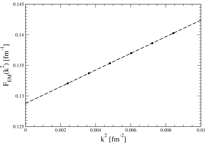
Figure 8: The effective range function of Eq. (143) for the potential model b with $(R_{\rm L},R_{\rm S})=(1.0,0.7)$ fm. The dashed line is a straight line fit.

The effective range function $F_{\rm EM}(k^{2})$ corresponding to model b is shown in Fig. 8. The numerical methods are stable down to lab energies of 1 keV.

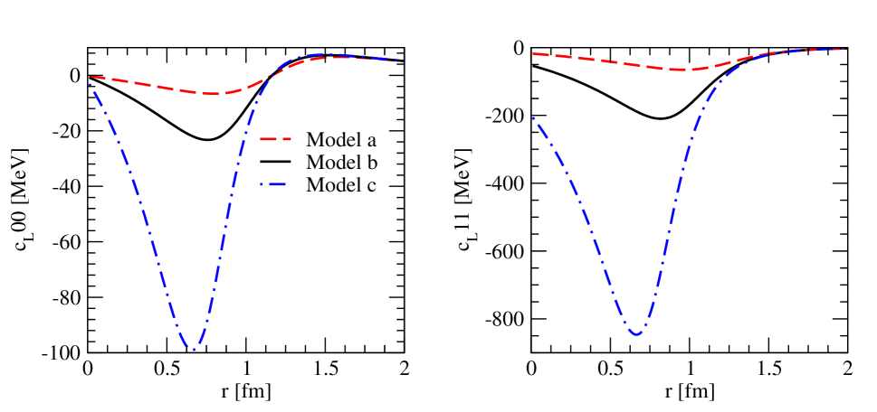
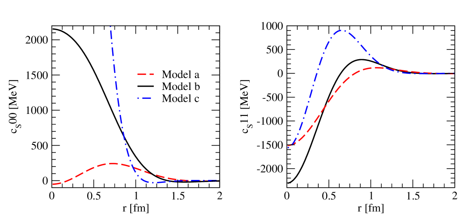
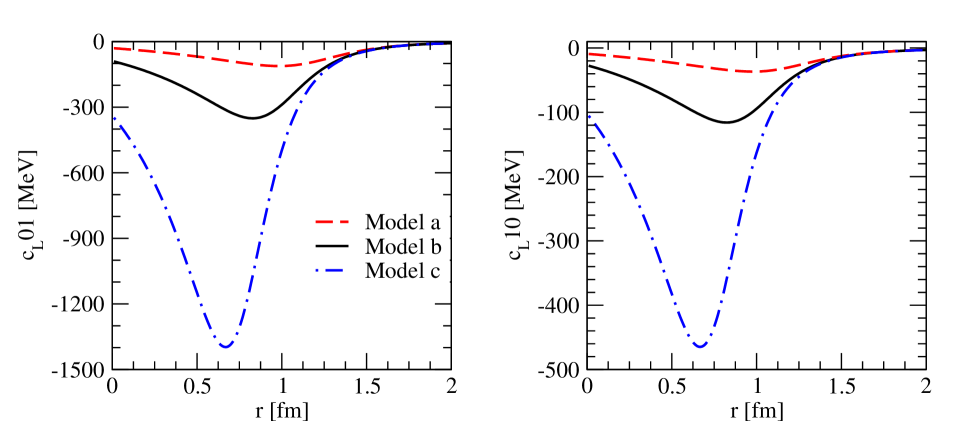
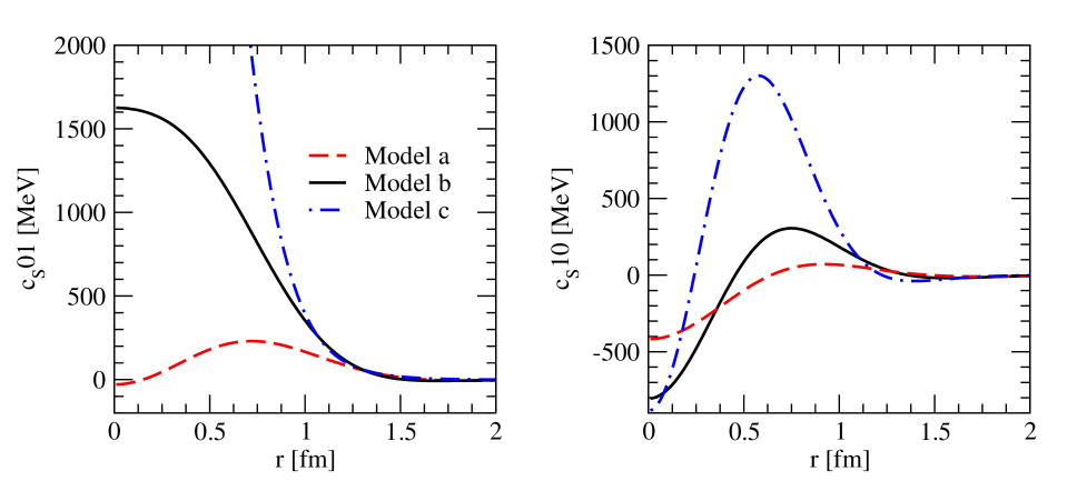
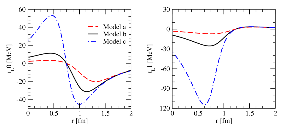
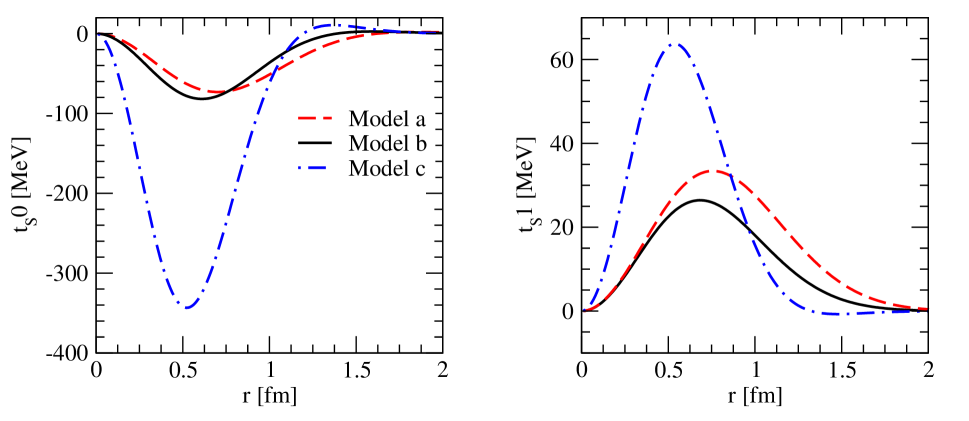
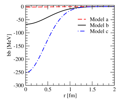
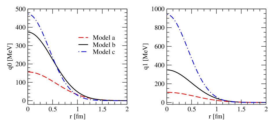
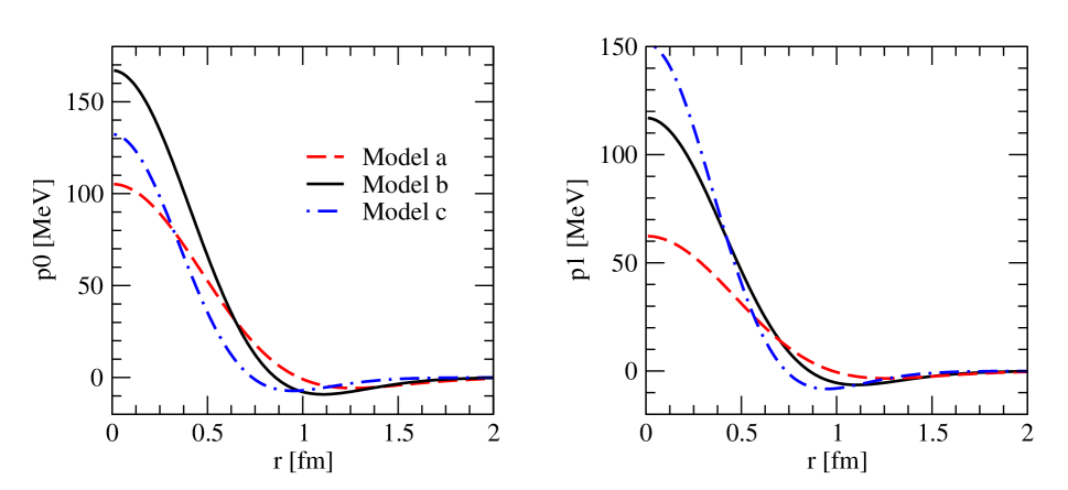
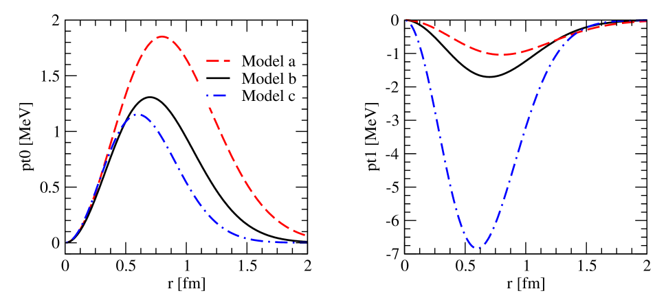
Appendix E Tables of phase shifts and figures of potential components

The $pp$ and $np$ phase shifts calculated with model b are listed in Tables 79, while the various components of the long-range ($v^{\rm L}_{12}$) and short-range ($v^{\rm S,CI}_{12}$) potentials corresponding to models a, b, and c and projected out in pair spin and isospin $S=0,1$ and $T=01$, are shown in Figs. 919.

Table 7: $pp$ phase shifts in degrees for potential model b with $(R_{\rm L},R_{\rm S})=(1.0,0.7)$ fm. The phases are relative to electromagnetic functions.
$E_{\rm lab}$ ${}^{1}S_{0}$ ${}^{1}D_{2}$ ${}^{1}G_{4}$ ${}^{3}P_{0}$ ${}^{3}P_{1}$ ${}^{3}F_{3}$ ${}^{3}P_{2}$ $\epsilon_{2}$ ${}^{3}F_{2}$ ${}^{3}F_{4}$
1 $32.69$ $0.00$ $0.00$ $0.14$ $-0.08$ $-0.00$ $0.02$ $-0.00$ $-0.00$ $0.00$
5 $55.00$ $0.04$ $0.00$ $1.64$ $-0.90$ $-0.00$ $0.22$ $-0.05$ $-0.01$ $0.01$
10 $55.49$ $0.17$ $0.00$ $3.90$ $-2.06$ $-0.03$ $0.64$ $-0.19$ $-0.01$ $0.02$
25 $49.13$ $0.69$ $0.04$ $9.21$ $-4.95$ $-0.23$ $2.42$ $-0.80$ $0.06$ $0.04$
50 $39.52$ $1.68$ $0.16$ $12.77$ $-8.38$ $-0.70$ $5.73$ $-1.71$ $0.27$ $0.14$
100 $25.66$ $3.77$ $0.43$ $11.21$ $-13.42$ $-1.58$ $11.02$ $-2.73$ $0.73$ $0.47$
150 $15.44$ $5.75$ $0.71$ $6.21$ $-17.63$ $-2.28$ $14.16$ $-3.05$ $1.10$ $0.97$
200 $7.20$ $7.38$ $1.01$ $0.50$ $-21.38$ $-2.90$ $15.90$ $-2.97$ $1.30$ $1.55$
250 $0.22$ $8.59$ $1.33$ $-5.18$ $-24.68$ $-3.52$ $16.89$ $-2.65$ $1.27$ $2.16$
300 $-5.88$ $9.36$ $1.66$ $-10.62$ $-27.55$ $-4.20$ $17.45$ $-2.19$ $0.98$ $2.76$
Table 8: $T=1$ $np$ phase shifts in degrees for potential model b with $(R_{\rm L},R_{\rm S})=(1.0,0.7)$ fm. The phases are relative to spherical Bessel functions.
$E_{\rm lab}$ ${}^{1}S_{0}$ ${}^{1}D_{2}$ ${}^{1}G_{4}$ ${}^{3}P_{0}$ ${}^{3}P_{1}$ ${}^{3}F_{3}$ ${}^{3}P_{2}$ $\epsilon_{2}$ ${}^{3}F_{2}$ ${}^{3}F_{4}$
1 $62.10$ $0.00$ $0.00$ $0.18$ $-0.11$ $-0.00$ $0.02$ $-0.00$ $0.00$ $0.00$
5 $63.65$ $0.04$ $0.00$ $1.67$ $-0.92$ $-0.00$ $0.24$ $-0.05$ $0.01$ $0.00$
10 $60.00$ $0.16$ $0.00$ $3.80$ $-2.02$ $-0.03$ $0.68$ $-0.19$ $0.02$ $0.00$
25 $50.83$ $0.67$ $0.03$ $8.71$ $-4.72$ $-0.20$ $2.53$ $-0.76$ $0.11$ $0.01$
50 $40.22$ $1.69$ $0.14$ $11.90$ $-7.88$ $-0.63$ $5.95$ $-1.63$ $0.33$ $0.08$
100 $25.84$ $3.86$ $0.40$ $10.06$ $-12.42$ $-1.46$ $11.35$ $-2.58$ $0.81$ $0.38$
150 $15.46$ $5.90$ $0.69$ $4.97$ $-16.17$ $-2.12$ $14.49$ $-2.81$ $1.20$ $0.84$
200 $7.13$ $7.58$ $1.00$ $-0.77$ $-19.50$ $-2.70$ $16.17$ $-2.64$ $1.44$ $1.41$
250 $0.09$ $8.81$ $1.33$ $-6.48$ $-22.43$ $-3.27$ $17.05$ $-2.24$ $1.45$ $2.01$
300 $-6.04$ $9.59$ $1.67$ $-11.93$ $-24.96$ $-3.89$ $17.49$ $-1.72$ $1.21$ $2.60$
Table 9: Same as in Table 8 but for $T=0$ $np$ phase shifts.
$E_{\rm lab}$ ${}^{1}P_{1}$ ${}^{1}F_{3}$ ${}^{3}D_{2}$ ${}^{3}G_{4}$ ${}^{3}S_{1}$ $\epsilon_{1}$ ${}^{3}D_{1}$ ${}^{3}D_{3}$ $\epsilon_{3}$ ${}^{3}G_{3}$
1 $-0.19$ $-0.00$ $0.01$ $0.00$ $147.81$ $0.10$ $-0.00$ $0.00$ $0.00$ $-0.00$
5 $-1.53$ $-0.01$ $0.22$ $0.00$ $118.32$ $0.63$ $-0.17$ $0.00$ $0.01$ $-0.00$
10 $-3.15$ $-0.07$ $0.85$ $0.01$ $102.80$ $1.06$ $-0.65$ $0.00$ $0.08$ $-0.00$
25 $-6.55$ $-0.43$ $3.70$ $0.17$ $80.86$ $1.53$ $-2.77$ $0.00$ $0.55$ $-0.04$
50 $-9.87$ $-1.16$ $8.89$ $0.73$ $63.00$ $1.62$ $-6.42$ $0.18$ $1.62$ $-0.25$
100 $-14.05$ $-2.33$ $17.21$ $2.20$ $43.53$ $1.67$ $-12.31$ $1.16$ $3.54$ $-0.97$
150 $-17.48$ $-3.12$ $22.33$ $3.71$ $31.32$ $1.92$ $-16.61$ $2.34$ $4.87$ $-1.88$
200 $-20.78$ $-3.69$ $25.02$ $5.10$ $22.35$ $2.34$ $-19.83$ $3.17$ $5.72$ $-2.83$
250 $-24.04$ $-4.14$ $26.09$ $6.36$ $15.26$ $2.84$ $-22.27$ $3.40$ $6.23$ $-3.76$
300 $-27.23$ $-4.56$ $26.10$ $7.46$ $9.40$ $3.39$ $-24.11$ $3.01$ $6.52$ $-4.62$
Refer to caption
Figure 9: (Color online) Central components of the long-range potential $v^{\rm L}_{12}$ in pair spin-isospin channels $ST=00$ and $11$.
Refer to caption
Figure 10: (Color online) Same as in Fig. 9, but for the short-range charge-independent potential $v^{\rm S,CI}_{12}$.
Refer to caption
Figure 11: (Color online) Same as in Fig. 9 but in pair spin-isospin channels $ST=01$ and $10$.
Refer to caption
Figure 12: (Color online) Same as in Fig. 10 but in pair spin-isospin channels $ST=01$ and $10$.
Refer to caption
Figure 13: (Color online) Tensor components of the long-range potential $v^{\rm L}_{12}$ in pair isospin channels $T=0$ and $1$.
Refer to caption
Figure 14: (Color online) Same as in Fig. 13 but for the short-range charge-independent potential $v^{\rm S,CI}_{12}$.
Refer to caption
Figure 15: (Color online) Spin-orbit components of the short-range charge-independent potential $v^{\rm S,CI}_{12}$ in pair isospin channels $T=0$ and $1$.
Refer to caption
Figure 16: (Color online) Spin and isospin independent quadratic spin-orbit components of the short-range charge-independent potential $v^{\rm S,CI}_{12}$.
Refer to caption
Figure 17: (Color online) Quadratic orbital angular momentum components of the short-range charge-independent potential $v^{\rm S,CI}_{12}$ in pair spin channels $S=0$ and $1$.
Refer to caption
Figure 18: (Color online) Quadratic relative momentum components of the short-range charge-independent potential $v^{\rm S,CI}_{12}$ in pair spin channels $S=0$ and $1$.
Refer to caption
Figure 19: (Color online) Quadratic-relative-momentum-tensor components of the short-range charge-independent potential $v^{\rm S,CI}_{12}$ in pair isospin channels $T=0$ and $1$.

References

  • (1) H.P. Stapp, T.J. Ypsilantis, and N. Metropolis, Phys. Rev.  105, 302 (1957).
  • (2) R.A. Arndt and M.H. MacGregor, Methods in Computational Physics 6, 253 (1966).
  • (3) V.G.J. Stoks, R.A.M. Klomp, M.C.M. Rentmeester, and J.J. de Swart, Phys. Rev. C 48, 792 (1993).
  • (4) V.G.J. Stoks, R.A.M. Klomp, C.P.F. Terheggen, and J.J. de Swart, Phys. Rev. C 49, 2950 (1994).
  • (5) R. B. Wiringa, V. G. J. Stoks, and R. Schiavilla, Phys. Rev. C 51, 38 (1995).
  • (6) M.C.M. Rentmeester, R.G.E. Timmermans, J.L. Friar, and J.J. de Swart, Phys. Rev. Lett.  82, 4992 (1999).
  • (7) R. Machleidt, Phys. Rev. C 63, 024001 (2001).
  • (8) M.C.M. Rentmeester, R.G.E. Timmermans, and J.J. de Swart, Phys. Rev. C 67, 044001 (2003).
  • (9) F.L. Gross and A. Stadler, Phys. Rev. C 78, 014005 (2008).
  • (10) R. Navarro Pérez, J.E. Amaro, and E. Ruiz Arriola, Phys. Rev. C 88, 064002 (2013).
  • (11) R. Navarro Pérez, J.E. Amaro, and E. Ruiz Arriola, Phys. Rev. C 89, 024004 (2014).
  • (12) R. Navarro Pérez, J.E. Amaro, and E. Ruiz Arriola, Phys. Rev. C 89, 064006 (2014).
  • (13) K. Chadan and P.C. Sabatier, Inverse Problems in Quantum Scattering Theory (Springer-Verlag, New York, 1989).
  • (14) D. Baye, J.M. Sparenberg, A.M. Pupasov-Maksimov, and B.F. Samsonov, J. Phys. A 47, 243001 (2014).
  • (15) S. K. Bogner, T. T. S. Kuo, A. Schwenk, D. R. Entem and R. Machleidt, Phys. Lett. B 576, 265 (2003)
  • (16) S. K. Bogner, T. T. S. Kuo and A. Schwenk, Phys. Rept.  386, 1 (2003)
  • (17) E. Ruiz Arriola, S. Szpigel and V. S. Timoteo, Annals Phys.  353, 129 (2014)
  • (18) J. Carlson, S. Gandolfi, F. Pederiva, S.C. Pieper, R. Schiavilla, K.E. Schmidt, and R.B. Wiringa, arXiv:1412.3081[nucl-th].
  • (19) T. Hatsuda, J. Phys. Conf. Ser.  381, 012020 (2012).
  • (20) W. Detmold, Lect. Notes Phys.  889, 153 (2015).
  • (21) R.A.M. Klomp, V.G.J. Stoks. and J.J. de Swart, Phys. Rev. C 44, 1258 (1991).
  • (22) S. Weinberg, Phys. Lett. B 251, 288 (1990).
  • (23) R. Machleidt and D.R. Entem, Phys. Rep. 503, 1 (2011).
  • (24) N. Kaiser, R. Brockmann, and W. Weise, Nucl. Phys. A 625, 758 (1997).
  • (25) S. Pastore, R. Schiavilla, and J.L. Goity Phys. Rev. C 78, 064002 (2008).
  • (26) R. Schiavilla, R.B. Wiringa, V.R. Pandharipande, and J. Carlson, Phys. Rev. C 45, 2628 (1992).
  • (27) M. Viviani, R. Schiavilla, and A. Kievsky, Phys. Rev. C 54, 534 (1996).
  • (28) L. Girlanda, A. Kievsky, L.E. Marcucci, S. Pastore, R. Schiavilla, and M. Viviani, Phys. Rev. Lett. 105, 232502 (2010).
  • (29) L.E. Marcucci, R. Schiavilla, M. Viviani, A. Kievsky, S. Rosati, and J.F. Beacom, Phys. Rev. C 63, 015801 (2001).
  • (30) J. Bystricky, F. Lehar, and P, Winternitz, J. Phys. 39, 1 (1978).
  • (31) J. Bystricky, C. Lechanoine-Leluc, and F. Lehar, J. Phys. 48, 199 (1987).
  • (32) D.R. Entem and R. Machleidt, Phys. Rev. C 68, 041001(R) (2003).
  • (33) E. Epelbaum, W. Glöckle, and U.-G. Meissner, Nucl. Phys. A 747, 362 (2005).
  • (34) D.R. Entem, N. Kaiser, R. Machleidt, and Y. Nosyk, Phys. Rev. C 91, 014002 (2015).
  • (35) E. Epelbaum, H. Krebs, and U.-G. Meissner, arXiv:1412.0142 [nucl-th].
  • (36) R. Navarro Perez, J.E. Amaro, and E. Ruiz Arriola, arXiv:1202.6624 [nucl-th].
  • (37) R. Navarro Perez, J.E. Amaro, and E. Ruiz Arriola, Phys. Lett. B 738, 155 (2014).
  • (38) R. Navarro Perez, J.E. Amaro, and E. Ruiz Arriola, PoS CD 12, 104 (2013).
  • (39) E. Epelbaum, W. Glöckle, and U.-G. Meissner, Nucl. Phys. A637, 107 (1998).
  • (40) S. Pastore, L. Girlanda, R. Schiavilla, M. Viviani, and R.B. Wiringa, Phys. Rev. C 80, 034004 (2009).
  • (41) M. Viviani, A. Baroni, L. Girlanda, A. Kievsky, L.E. Marcucci, and R. Schiavilla, Phys. Rev. C 89, 064004 (2014).
  • (42) N. Kaiser, S. Gerstendörfer, and W. Weise Nucl. Phys. A 637, 395 (1998).
  • (43) H. Krebs, E. Epelbaum, and Ulf.-G. Meißner, Eur. Phys. J. A 32, 127 (2007).
  • (44) E. Epelbaum, W. Glöckle, and U.-G. Meißner, Eur. Phys. J. A 19, 125 (2004).
  • (45) A.M. Green, Rep. Prog. Phys. 39, 1109 (1976).
  • (46) N. Fettes, U.-G. Meissner, M. Mojz̆is̆, S. Steininger, Ann. Phys. 283, 273 (2000).
  • (47) M. Pavón Valderrama and E. Ruiz Arriola, Phys. Rev. C 79, 044001 (2009).
  • (48) M. Pavón Valderrama and E. Ruiz Arriola, Phys. Rev. C 83, 044002 (2011).
  • (49) J.L. Friar, U. van Kolck, M.C.M. Rentmeester, and R.G.E. Timmermans, Phys. Rev. C 70, 044001 (2004).
  • (50) E. Epelbaum and U.-G. Meissner, Phys. Rev. C 72, 044001 (2005).
  • (51) U. van Kolck, M.C.M. Rentmeester, J.L. Friar, T. Goldman, and J.J. de Swart, Phys. Rev. Lett. 80, 4386 (1998).
  • (52) N. Kaiser, Phys. Rev. C 73, 044001 (2006).
  • (53) A. Gezerlis, I. Tews, E. Epelbaum, S. Gandolfi, K. Hebeler, A. Nogga, and A. Schwenk, Phys. Rev. Lett. 111, 032501 (2013); A. Gezerlis, I. Tews, E. Epelbaum, M. Freunek, S. Gandolfi, K. Hebeler, A. Nogga, and A. Schwenk, Phys. Rev. C 90, 054323 (2014).
  • (54) V.G.J. Stoks and J.J. de Swart, Phys. Rev. C 42, 1235 (1990).
  • (55) M. Kortelainen, T. Lesinski, J. More, W. Nazarewicz, J. Sarich, N. Schunck, M.V. Stoitsov, and S. Wild, Phys. Rev. C 82, 024313 (2010).
  • (56) G.A. Miller, M.K. Nefkens, and I. Slaus, Phys. Rep. 194, 1 (1990).
  • (57) R. Machleidt, Phys. Rev. C 63, 024001 (2001).
  • (58) D.E. González Trotter et al., Phys. Rev. C 73, 034001 (2006).
  • (59) Q. Chen et al., Phys. Rev. C 77, 054002 (2008).
  • (60) C. van der Leun and C. Alderlisten, Nucl. Phys. A 380, 261 (1982).
  • (61) T.E.O. Ericson and M. Rosa-Clot, Nucl. Phys. A 405, 497 (1983).
  • (62) N.L. Rodning and L.D. Knutson, Phys. Rev. C 41, 898 (1990).
  • (63) A. Huber et al., Phys. Rev. Lett. 80, 468 (1998).
  • (64) D.M. Bishop and L.M. Cheung, Phys. Rev. A 20, 381 (1979).
  • (65) M. Piarulli, L. Girlanda, L.E. Marcucci, S. Pastore, R. Schiavilla, and M. Viviani, Phys. Rev. C 87, 014006 (2013).
  • (66) A. Kievsky, S. Rosati, M. Viviani, L.E. Marcucci, and L. Girlanda, J. Phys. G 35, 063101 (2008).
  • (67) R. N. Perez, J. E. Amaro and E. R. Arriola, arXiv:1411.1212 [nucl-th].
  • (68) J.R. Bergervoet, P.C. van Campen, W.A. van de Sanden, and J.J. de Swart, Phys. Rev. C 38, 15 (1988).
  • (69) L. Heller, Phys. Rev. 120, 627 (1960).
  • (70) W.A. van de Sanden, A.H. Emmen, J.J. de Swart, Report No. THEF-NYM-83.11, Nijmegen (1983), unpublished; quoted in Berg88 .