Validity of ChPT – is $\;M_{\pi}=135\,\mathrm{MeV}\;$ small enough ?

Abstract:

I discuss the practical convergence of the SU(2) ChPT series in the meson sector, based on 2+1 flavor lattice data by the Wuppertal-Budapest and Budapest-Marseille-Wuppertal collaborations. These studies employ staggered and clover-improved Wilson fermions, respectively. In both cases large box volumes and several lattice spacings are used, and the pion masses reach down to the physical mass point. We conclude that LO and NLO low-energy constants can be determined with controlled systematics, if there is sufficient data between the physical mass point and about $350\,\mathrm{MeV}$ pion mass. Exploratory LO+NLO+NNLO fits with a wider range reveal some distress of the chiral series near $M_{\pi}\sim 400\,\mathrm{MeV}$ and suggest a complete breakdown beyond $M_{\pi}\sim 500\,\mathrm{MeV}$.

1 Introduction

Lattice QCD (LQCD) is the ab-initio approach to strong interactions, valid for any value of the gauge coupling. Chiral Perturbation Theory (ChPT) is the effective field theory approach to the same set of phenomena, valid for small quark masses, small momenta and large box-sizes.

The chiral framework is set up as an expansion about the 2-flavor or 3-flavor massless limit. The SU(2) Lagrangian [1] contains two low-energy constants (LECs) at the leading order (LO), the pion decay constant $F$ and the condensate parameter $B\!=\!\Sigma/F^{2}$, both defined via $m_{u,d}\!\to\!0$ and sometimes denoted $F^{(2)},B^{(2)}$, seven LECs at the NLO, $\bar{\ell}_{1..7}\!\equiv\!\ln(\Lambda_{1..7}^{2}/[135\!\,\mathrm{MeV}]^{2})$, as well as a large number of LECs at the NNLO. The SU(3) Lagrangian [2] contains two LECs at the leading order, $F$ and $B\!=\!\Sigma/F^{2}$, both defined via $m_{u,d,s}\!\to\!0$ and sometimes denoted $F^{(3)},B^{(3)}$, ten LECs at the NLO, $L_{1..10}^{\mathrm{ren}}(\mu\!\sim\!770\,\mathrm{MeV})$, and a large number of LECs at the NNLO. Below I will use $f$ and $F\!=\!f/\sqrt{2}$ in parallel, with $f_{\pi}^{\mathrm{phys}}\!\simeq\!130.4\,\mathrm{MeV}$ and $F_{\pi}^{\mathrm{phys}}\!\simeq\!92.2\,\mathrm{MeV}$.

In phenomenology, the convergence pattern is governed by the value of $m_{ud}^{\mathrm{phys}}\simeq 3.5\,\mathrm{MeV}$ [in ${\overline{\mathrm{MS}}}$ scheme at $\mu\!=\!2\,\mathrm{GeV}$] in the SU(2) framework, and by the value of $m_{s}^{\mathrm{phys}}\simeq 95\,\mathrm{MeV}$ in the SU(3) framework. The SU(2) LECs depend implicitly on $m_{s}^{\mathrm{phys}}$ (and heavier flavors), and the SU(3) LECs depend implicitly on $m_{c}^{\mathrm{phys}}$ (and heavier flavors).

The lattice can help phenomenology by determining the numerical values of the LECs from first principles. Conversely, chiral formulas can aid the lattice, since they connect different channels. However, by using chiral formulas, one implicitly performs an extrapolation to the respective chiral limit, and this opens the question whether the data used are suitable to sustain that limit. This proceedings contribution is about the selection of appropriate mass ranges (in $M_{\pi}^{2}$ or $m_{ud}$, and possibly $2M_{K}^{2}\!-\!M_{\pi}^{2}$ or $m_{s}$) to perform the matching between the lattice data and the chiral formulas such that the relevant LECs can be determined with controlled systematic uncertainties.

2 Features of ChPT

2.1 SU(2) and SU(3) ChPT versus 2 and 2+1 and 2+1+1 flavor lattice data

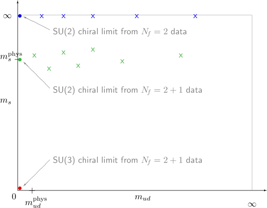
Figure 1: Sketch of different data taking strategies in the $(m_{ud},m_{s})$ plane. Simulations of QCD with $N_{\!f}=2$ work effectively at $m_{s}=\infty$. Most $N_{\!f}=2+1$ simulations use $m_{s}$ values in the vicinity of $m_{s}^{\mathrm{phys}}$; for a controlled extrapolation to the SU(3) chiral limit additional data with $m_{s}\ll m_{s}^{\mathrm{phys}}$ are mandatory.

With $N_{\!f}=2$ lattice data in hand one can only attempt to match to SU(2) ChPT. The resulting LECs are logically different from those in phenomenology, since they do not know about $m_{s}^{\mathrm{phys}}$, though the difference may be numerically small. With $N_{\!f}=2+1$ or $N_{\!f}=2+1+1$ data one has, in principle, the choice to match to SU(2) or SU(3) ChPT. Many collaborations opt for generating such ensembles with $m_{s}\simeq m_{s}^{\mathrm{phys}}$, see Fig.1. In the event that there is no significant “lever-arm” in $m_{s}$, one is restricted to comparing with SU(2) ChPT. The advantage compared to $N_{\!f}=2$ studies is that this time the LECs agree with those in phenomenology (up to effects $\propto\!1/m_{c}^{2}$ or $\propto\!1/m_{b}^{2}$).

2.2 Chiral expansion in $x$ versus in $\xi$

Chiral formulas are often presented as an expansion in the quark mass, for instance

$$M_{\pi}^{2}\! \!=\! \!M^{2}\,\bigg{\{}1+\frac{1}{2}x\ln\frac{M^{2}}{\Lambda_{3}^{2}}+\frac{17}{8}x^{2}\Big{(}\!\ln\frac{M^{2}}{\Lambda_{M}^{2}}\Big{)}^{2}+x^{2}k_{M}+O(x^{3})\bigg{\}}$$ (1)

$$F_{\pi}\! \!=\! \!F\;\;\;\bigg{\{}1-x\ln\frac{M^{2}}{\Lambda_{4}^{2}}-\frac{5}{4}x^{2}\Big{(}\!\ln\frac{M^{2}}{\Lambda_{F}^{2}}\Big{)}^{2}+x^{2}k_{F}+O(x^{3})\bigg{\}}\;,$$ (2)

where $x\equiv M^{2}/(4\pi F)^{2}$ with $M^{2}\equiv B(m_{1}\!+\!m_{2})$. In lattice analyses it may be convenient to invert these formulas such that they are an expansion in $\xi\equiv M_{\pi}^{2}/(4\pi F_{\pi})^{2}=M_{\pi}^{2}/(8\pi^{2}f_{\pi}^{2})$, whereupon

$$M^{2}\! \!=\! \!M_{\pi}^{2}\,\bigg{\{}1-\frac{1}{2}\xi\ln\frac{M_{\pi}^{2}}{\Lambda_{3}^{2}}-\frac{5}{8}\xi^{2}\Big{(}\!\ln\frac{M_{\pi}^{2}}{\Omega_{M}^{2}}\Big{)}^{2}+\xi^{2}c_{M}+O(\xi^{3})\bigg{\}}$$ (3)

$$F\! \!=\! \!F_{\pi}\;\;\bigg{\{}1+\xi\ln\frac{M_{\pi}^{2}}{\Lambda_{4}^{2}}-\frac{1}{4}\xi^{2}\Big{(}\!\ln\frac{M_{\pi}^{2}}{\Omega_{F}^{2}}\Big{)}^{2}+\xi^{2}c_{F}+O(\xi^{3})\bigg{\}}\;.$$ (4)

The scales $\Lambda_{3,4}$ and $\Lambda_{M,F}$ or $\Omega_{M,F}$ carry no quark mass dependence (w.r.t. the explicitly treated flavors) and no scale dependence. More details, e.g. the relation $\Lambda_{M,F}\leftrightarrow\Omega_{M,F}$, are found in [3]. Some of the early discussion of the issue “$x$ versus $\xi$ expansion” is found in [4, 5, 6].

2.3 Curvature and chiral logarithms

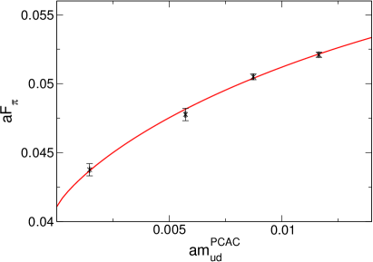
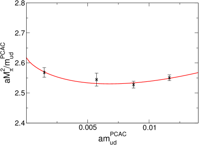
Figure 2: Typical example of possible curvature in $aF_{\pi}$ and $aM_{\pi}^{2}/m_{ud}$ versus $am_{ud}$. Figure taken from [8].

Evidently, chiral logs are linked to the curvature inherent in data that follow the chiral prediction (1, 2), see e.g. Fig. 2. Naively, one might guess that the location of the curvature in a standard chiral logarithm $f(M^{2})=M^{2}\log(M^{2}/\Lambda_{i}^{2})$ is linked to the scale $\Lambda_{i}$. However, taking derivatives yields $f^{\prime}(M^{2})=\log(M^{2}/\Lambda_{i}^{2})+1$ and hence $f^{\prime\prime}(M^{2})=1/M^{2}$. In other words, the curvature grows monotonically towards the chiral limit, and this means that one needs data sufficiently close to the chiral limit to be able to discriminate $f^{\prime\prime}(M^{2})$ against zero (with the given statistics).

2.4 Warning about finite volume effects

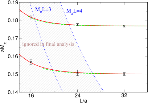
Figure 3: Illustration of $aM_{\pi}(L)>aM_{\pi}$ for two values of $am_{ud}$ at fixed $\beta$. Figure taken from [8], in which only the three data-points with $M_{\pi}(L)L>4$ would enter the final analysis.

In LQCD we work in euclidean boxes $L^{3}\!\times\!T$, and the finite spatial extent $L$ creates a potential threat to the chiral expansion. With periodic boundary conditions the lowest non-trivial momentum is $p_{\mathrm{min}}=2\pi/L$. With $L=2\,\mathrm{fm}$ one has $p_{\mathrm{min}}\simeq 630\,\mathrm{MeV}$, which is likely too much.

We are predominantly interested in the $p$-regime where $L^{-1}\ll M_{\pi}\ll 4\pi F_{\pi}$, and the counting rule reads $m_{q}\sim M_{\pi}^{2}\sim p^{2}\sim L^{-2}$. ChPT at the one-loop order predicts the finite volume effects [7]

$$M_{\pi}(L) = M_{\pi}\,\Big{\{}1+\frac{1}{2N_{\!f}}\xi\tilde{g}_{1}(M_{\pi}L)+O(\xi^{2})\Big{\}}$$ (5)

$$F_{\pi}(L) = \,F_{\pi}\,\,\Big{\{}1-\frac{N_{\!f}}{2}\,\xi\,\tilde{g}_{1}(M_{\pi}L)+O(\xi^{2})\,\Big{\}}$$ (6)

where the shape function $\tilde{g}_{1}$ is given as an expansion in terms of a Bessel function

$$\tilde{g}_{1}(z) = \frac{24}{z}K_{1}(z)+\frac{48}{\sqrt{2}z}K_{1}(\sqrt{2}z)+\frac{32}{\sqrt{3}z}K_{1}(\sqrt{3}z)+\frac{24}{2z}K_{1}(2z)+...$$ (7)

$$K_{1}(z) = \sqrt{\frac{\pi}{2z}}\,e^{-z}\,\Big{\{}1+\frac{3}{8z}-\frac{3\cdot 5}{2(8z)^{2}}+\frac{3\cdot 5\cdot 21}{6(8z)^{3}}-\frac{3\cdot 5\cdot 21\cdot 45}{24(8z)^{4}}+...\Big{\}}\;.$$ (8)

Finite-volume effects such as those shown in Fig. 3 might grow towards the chiral limit and might mimic chiral logs. For a given set of data one wants to know whether some curvature remains after the finite-volume effects have been compensated for. The rule of thumb is that data with $M_{\pi}L\geq 4$ and $L\geq 3\,\mathrm{fm}$ can be corrected for finite-volume effects by means of ChPT formulas.

3 Investigation with staggered fermions

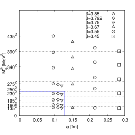
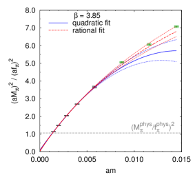
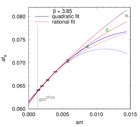
Figure 4: Overview of the “landscape” of simulation data available for the staggered investigation (left). For each $\beta$-value $M_{\pi}^{2}/f_{\pi}^{2}$ is interpolated or extrapolated, with a polynomial or rational function in $am_{ud}$, to the point where this ratio equals 1.06846; this yields $(am)^{\mathrm{phys}}$ (middle). For each $\beta$-value the polynomial or rational function $af_{\pi}$ is evaluated at $(am)^{\mathrm{phys}}$; identifying this $f_{\pi}$ with $f_{\pi}^{\mathrm{PDG}}$ yields $a$ (right).

The first investigation to be presented [9] uses staggered fermions. Fig. 4 shows that six lattice spacings are available, each of which features one ensemble with $M_{\pi}\simeq 135\,\mathrm{MeV}$. The 2nd and 3rd panel illustrate how the physical light quark mass and the lattice spacing are determined.

3.1 Joint SU(2) chiral fit at NLO

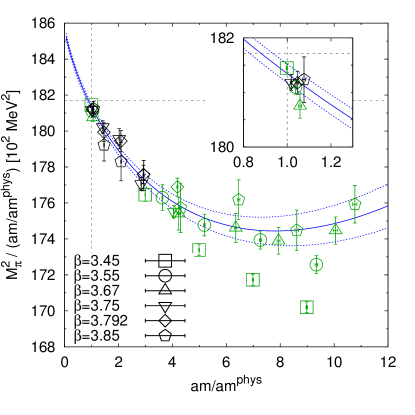
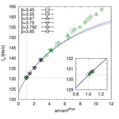
Figure 5: Our preferred joint LO+NLO fit to $M_{\pi}^{2}=M_{\pi}^{2}(m)$ and $f_{\pi}=f_{\pi}(m)$ uses data with $a^{-1}>1.6\,\mathrm{GeV}$ and $M_{\pi}<240\,\mathrm{MeV}$ (black data). The green data are shown for comparison; they are not used in the fit.

The goal is to determine $\bar{\ell}_{3,4}$ from a joint fit to the data shown in Fig. 5. After a two-fold cut, for instance $a^{-1}\!<\!1.6\,\mathrm{GeV}$ and $M_{\pi}\!<\!240\,\mathrm{MeV}$, the data can be fitted with the continuum NLO formulas (1, 2). The non-coarse green data deviate for $m_{ud}>5m_{ud}^{\mathrm{phys}}$ or $M_{\pi}>300\,\mathrm{MeV}$.

3.2 Sensitivity of LECs on chiral range

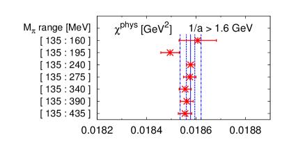
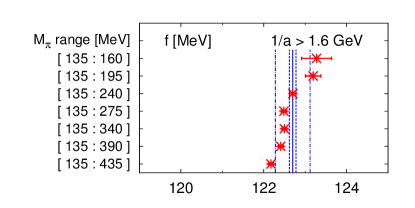
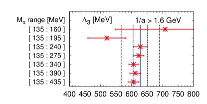
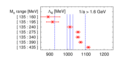
Figure 6: Summary of fitted LO ($B$ or $\chi^{\mathrm{phys}}\!\equiv\!2Bm_{ud}^{\mathrm{phys}}$, $f$) and NLO ($\Lambda_{3}$, $\Lambda_{4}$) low-energy constants, with $M_{\pi}^{\mathrm{min}}=135\,\mathrm{MeV}$ and $a^{-1}>1.6\,\mathrm{GeV}$ and several $M_{\pi}^{\mathrm{max}}$. The three inner lines indicate the respective central value and statistical error that come from the preferred fit ($M_{\pi}^{\mathrm{max}}=240\,\mathrm{MeV}$). The scatter of all results gives the systematic uncertainty which, when added in quadrature to the statistical error, yields the outer band.

Our preferred fit features $M_{\pi}^{\mathrm{max}}=240\,\mathrm{MeV}$. It is of paramount importance to compare its output to the parameters obtained with smaller and larger $M_{\pi}^{\mathrm{max}}$, in order to arrive at a reliable estimate of the theoretical uncertainty that comes from the chiral range used, see Fig. 6.

3.3 Sensitivity on cuts from above/below

One of the real benefits of a dataset that reaches down to the physical mass point is that we can artificially prune the data from below and observe how much of an effect this has on the fitted LO and NLO parameters. Some of this comparison is shown in Fig. 7. Quite generally, $\chi$ and $\bar{\ell}_{3}$ are fairly robust against variations of the chiral range, while $f$ and $\bar{\ell}_{4}$ are far more sensitive. Choosing $M_{\pi}^{\mathrm{min}}$ too large tends to yield $f$ values which are too low and $\bar{\ell}_{4}$ values which are too high.

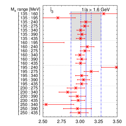
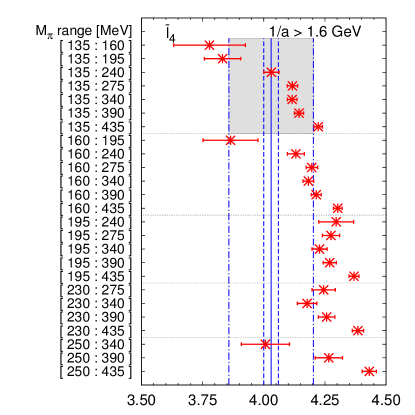
Figure 7: Comparison of the NLO fits shown in the previous figure (top panel, gray underlay) to those with $M_{\pi}^{\mathrm{min}}=160,195,230,250\,\mathrm{MeV}$ (lower four panels).

3.4 Breakup into LO/NLO/NNLO parts

One of the most interesting games that one can play with such a data set is an exploratory fit that includes the NNLO terms of equation (1, 2). The low-energy constants $\Lambda_{M,F}$ are determined through powers of $\Lambda_{1,2}$ (which are well known from phenomenology) and $\Lambda_{3,4}$ (which are determined through the NLO part of the fit under discussion); only $k_{M,F}$ are genuinely new. As a result, it makes sense to include the knowledge on $\Lambda_{1,2}$ as a prior. Still, to prevent instabilities, the fit range must be chosen somewhat wider than in the case of the LO+NLO fit.

Fig. 8 shows the break-up of the LO+NLO+NNLO fit into its LO-part (green) LO+NLO-part (red) and the full thing (blue). At $m_{ud}=m_{ud}^{\mathrm{phys}}$ we find an excellent convergence pattern, that is $|\mathrm{NNLO}|\ll|\mathrm{NLO}|$. At $m_{ud}=7m_{ud}^{\mathrm{phys}}$ or $M_{\pi}\!\sim\!350\,\mathrm{MeV}$ we find $|\mathrm{NNLO}|\simeq\frac{1}{2}|\mathrm{NLO}|$, which marks the beginning of some distress on the chiral series. At $m_{ud}\simeq 11m_{ud}^{\mathrm{phys}}$ or $M_{\pi}\!\sim\!450\,\mathrm{MeV}$ the ordering seems to get lost, and the chiral expansion breaks down.

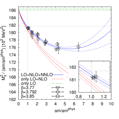
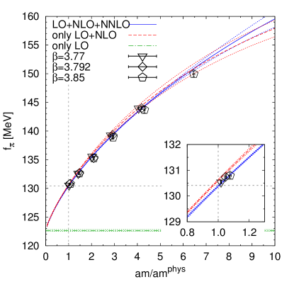
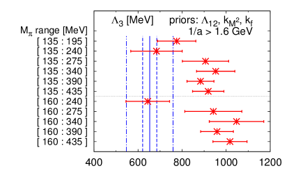
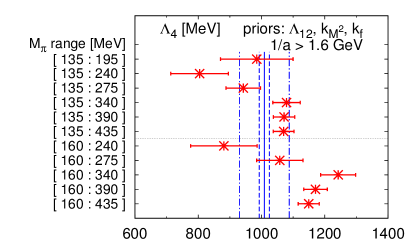
Figure 8: Top: Break-up of the joint LO+NLO+NNLO fit into its LO-part (green) LO+NLO-part (red) and the full thing (blue). Bottom: Comparing the resulting $\Lambda_{3,4}$ to those from Fig. 6 (indicated by the blue lines).

4 Investigation with Wilson fermions

The second investigation to be presented [10] uses tree-level clover improved Wilson fermions. Again, we use only data with $m^{\mathrm{sea}}=m^{\mathrm{val}}$. The presence of additive quark mass renormalization invites employing a global fit. This, in turn, suggests studying the issue of $x$ versus $\xi$ expansion.

4.1 NLO fit via $x$ and $\xi$ expansion

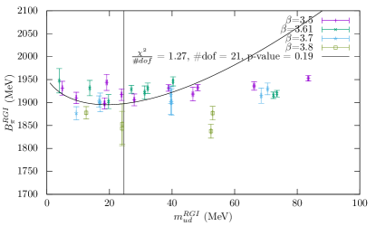
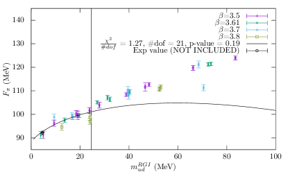
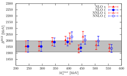
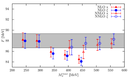
Figure 9: Top: $x$ expansion fit at NLO of $M_{\pi}^{2}/m_{ud}$ and $F_{\pi}$ versus $m_{ud}$ with $M_{\pi}^{\mathrm{max}}=300\,\mathrm{MeV}$. Bottom: fit parameters $B,F$ as a function of $M_{\pi}^{\mathrm{max}}$.

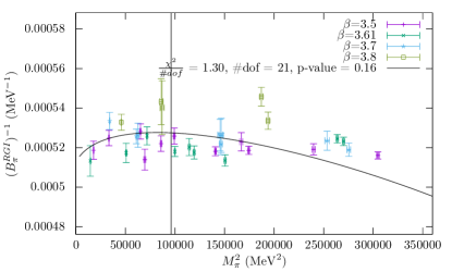
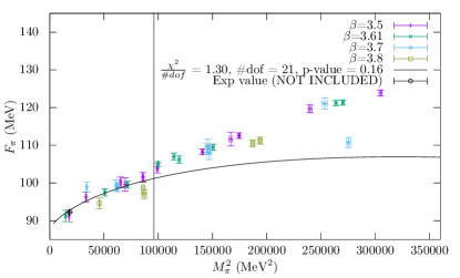
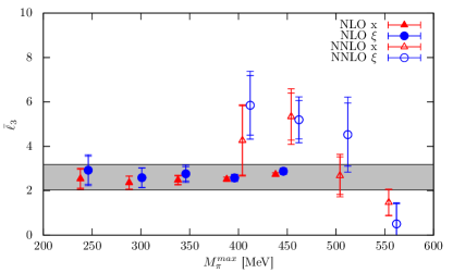
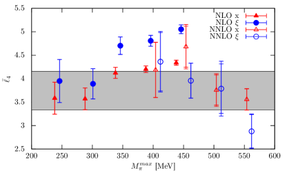
Figure 10: Top: $\xi$ expansion fit at NLO of $m_{ud}/M_{\pi}^{2}$ and $F_{\pi}$ versus $M_{\pi}^{2}$ with $M_{\pi}^{\mathrm{max}}=300\,\mathrm{MeV}$. Bottom: fit parameters $\bar{\ell}_{3},\bar{\ell}_{4}$ as a function of $M_{\pi}^{\mathrm{max}}$.

We perform joint LO+NLO fits, this time in the $x$ and $\xi$ expansion, and monitor how parameters shift as a function of $M_{\pi}^{\mathrm{max}}$. Fig. 9 shows our results for the LECs at the LO; $B$ is fairly insensitive to this cut, while $F$ is significantly affected if $M_{\pi}^{\mathrm{max}}>300\,\mathrm{MeV}$. Fig. 10 shows our results for the LECs at the NLO; $\bar{\ell}_{3}$ is fairly robust, while $\bar{\ell}_{4}$ shows a clear trend. All these findings are in complete analogy to what was found in the staggered case. A new ingredient is that we can now compare the $x$ and the $\xi$ expansion results (red triangles versus blue bullets) in case there is a drift. For $F$ there is no discrepancy (last panel of Fig. 9), while for $\bar{\ell}_{4}$ the onset of a discrepancy seems to signal the end of the regime where NLO ChPT is applicable (last panel of Fig. 10).

4.2 NNLO fit via $x$ and $\xi$ expansion

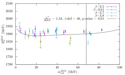
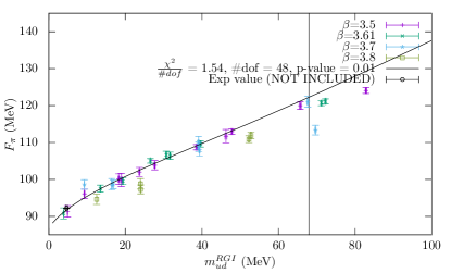
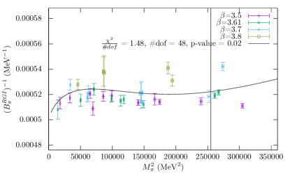
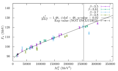
Figure 11: LO+NLO+NNLO fit in $x$ expansion (top) or $\xi$ expansion (bottom) of $M_{\pi}^{2}/m_{ud}$ or $m_{ud}/M_{\pi}^{2}$ (left) and $F_{\pi}$ (right) versus $m_{ud}$ or $M_{\pi}^{2}$, respectively.

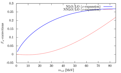
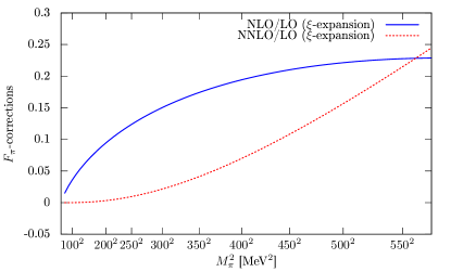
Figure 12: Breakup of LO+NLO+NNLO fit in $x$ or $\xi$ expansion to give NLO/LO and NNLO/LO ratios.

Given the large dataset, we attempt a provisional LO+NLO+NNLO fit. It is clear that such fits necessitate the inclusion of somewhat higher $M_{\pi}^{\mathrm{max}}$ values, see Fig. 11. We are not interested in the LECs at the NNLO, but rather how the LO and NLO counterparts compare to those obtained from the direct LO+NLO fit. The open symbols in Fig. 9 and Fig. 10 indicate that they tend to come with larger statistical errors, but within errors they are reasonably consistent with the earlier results.

Once more we can break up the complete fit into its LO, NLO, and NNLO contributions, and compare their relative importance. From Fig. 12 we learn that in $F_{\pi}=F_{\pi}(m_{ud})$ or $F_{\pi}=F_{\pi}(M_{\pi}^{2})$ the NLO contribution stays saturated at about 25% of the LO contribution, but the NNLO/NLO ratio exceeds $\frac{1}{2}$ at about $M_{\pi}\sim 450\,\mathrm{MeV}$ (which is a first sign of distress), and exceeds $1$ at about $M_{\pi}\sim 550\,\mathrm{MeV}$ (which clearly signals the breakdown of the chiral expansion). These results are again in qualitative agreement with what was found in the staggered case.

4.3 Sensitivity of LO+NLO fit on pruning data from below

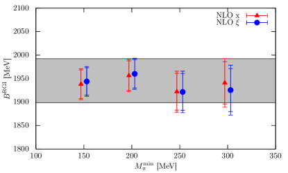
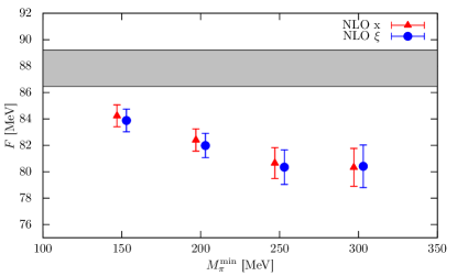
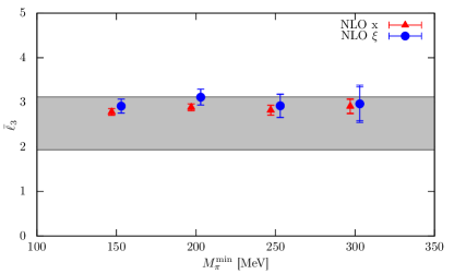
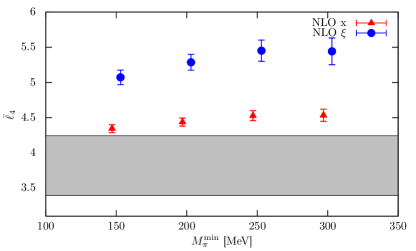
Figure 13: Sensitivity of LO (top) and NLO (bottom) low-energy constants on $M_{\pi}^{\mathrm{min}}$ in LO+NLO fits.

Fig. 13 shows the results for $B,F$ (top) as well as $\bar{\ell}_{3},\bar{\ell}_{4}$ (bottom) as a function of $M_{\pi}^{\mathrm{min}}$. We find that $B,\bar{\ell}_{3}$ are fairly robust, while $F,\bar{\ell}_{4}$ tend to come out too low and too high, respectively, in view of results that include our more chiral data (indicated by the gray bands). Again, the discrepancy between $x$ and $\xi$ expansion may signal an inappropriate mass range ($\bar{\ell}_{4}$) but need not do so ($F$).

5 FLAG review of LECs in SU(2) and SU(3) ChPT

Though this is a topical contribution, it might be adequate to highlight the FLAG summary [3] of LECs to show that there are several fine lattice calculations of LECs in SU(2) and SU(3) ChPT.

5.1 Summary of SU(2) LECs at NLO

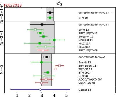
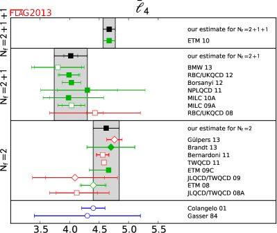
Figure 14: Summary of the SU(2) NLO low-energy constants $\bar{\ell}_{3}$ and $\bar{\ell}_{4}$ as compiled by FLAG [3].

Fig. 14 shows the FLAG compilation of SU(2) LECs at the NLO. The results are grouped into the categories $N_{\!f}=2$, $N_{\!f}=2+1$, and $N_{\!f}=2+1+1$. In addition, one or two phenomenological calculations of high standing are added for comparison. Some of the results are shown with red symbols, because one ingredient of the calculation is not state-of-the-art (e.g. data do not probe the chiral regime, or just one lattice spacing is used). Results which passed such quality checks are represented by green symbols. A filled symbol indicates that the result did enter the FLAG recommended value, an open symbol means that it did not (e.g. because the paper is not yet published or because it has been superseded by a more recent result by the same collaboration).

FLAG aims for very conservative error estimates. A standard mathematical average is formed, but then the error is stretched until the gray $\pm 1\sigma$ band covers the central values of all calculations which entered. This is done for each $N_{\!f}$ so that one can observe a potential $N_{\!f}$ dependence.

Concerning $\bar{\ell}_{3}$ the lattice approach is a success story. The results from $N_{\!f}=2$, $N_{\!f}=2+1$ and $N_{\!f}=2+1+1$ studies are consistent, and they achieve better precision than the phenomenological estimate “Gasser 84”. For $\bar{\ell}_{4}$ the situation is more challenging. For each $N_{\!f}$ the lattice results seem consistent, but there is a remnant dependence on whether a strange and/or charm quark is included in the sea. In principle, such an $N_{\!f}$ dependence is possible, but one would expect it to be monotonic. In addition, the lattice has difficulties in beating “Colangelo 01” in terms of precision.

5.2 Summary of SU(3) LECs at NLO

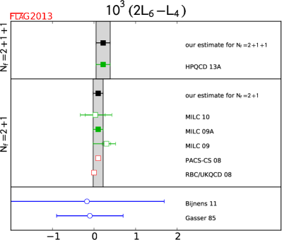
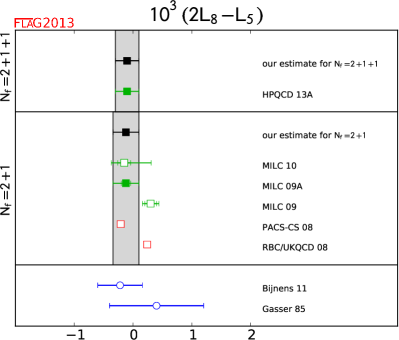
Figure 15: Summary of the SU(3) NLO low-energy constant combinations $2L_{6}^{\mathrm{ren}}-L_{4}^{\mathrm{ren}}$ and $2L_{8}^{\mathrm{ren}}-L_{5}^{\mathrm{ren}}$ as compiled by FLAG [3]. The renormalization scale is $\mu\sim 770\,\mathrm{MeV}$, as is customary in phenomenology.

Fig. 15 shows the FLAG compilation of SU(3) LECs at the NLO. The results are grouped into the categories $N_{\!f}=2+1$ and $N_{\!f}=2+1+1$. Again, one or two phenomenological calculations of high standing are added for comparison. The main difference to the SU(2) case is that there are fewer lattice determinations. This is not so much an effect of few collaborations generating $N_{\!f}=2+1$ ensembles, but of the requirement that, in order to control the SU(3) expansion, some ensembles with $m_{s}\ll m_{s}^{\mathrm{phys}}$ must be available (compare the discussion in Sec. 1 and Subsec. 2.1).

The situation looks quite favorable for the lattice approach, for both $2L_{6}-L_{4}$ and $2L_{8}-L_{5}$. The lattice results seem reasonably consistent, there is no visible $N_{\!f}$ dependence, and the latest generation of results is significantly more precise than the best phenomenological determinations.

In the future one would like to see tests of the large-$N_{\!c}$ prediction $L_{4,6}\to 0$, and one would like to see precision results for the flavor breaking ratios $F^{(2)}/F^{(3)}$, $\Sigma^{(2)}/\Sigma^{(3)}$, $B^{(2)}/B^{(3)}$, in order to test the Zweig rule (see Ref. [3] for details). As discussed in Subsec. 2.1 such studies require two different chiral limits to be performed from one set of $N_{\!f}=2+1$ or $N_{\!f}=2+1+1$ data.

6 Assorted remarks

Let me finish this proceedings contribution with two brief remarks – one concerning the way how LECs are calculated, one concerning the impact of a growing number of light flavors.

6.1 Rationale for log-free compounds

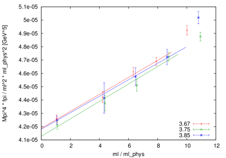
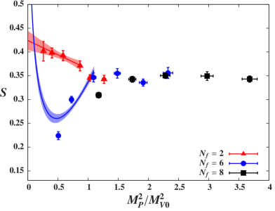
Figure 16: Left: $M_{\pi}^{4}f_{\pi}/m_{ud}^{2}$ as a function of $m_{ud}$, with quark masses normalized by $m_{ud}^{\mathrm{phys}}$, at the three finest lattice spacings of Ref. [9]. Right: $S$-parameter for $N_{\!f}=2,6,8$ as a function of $M_{P}^{2}/M_{V}^{2}$ from Ref. [11].

As discussed in Sec. 3 and Sec. 4 the dominant source of systematic uncertainty in a lattice determination of ChPT LECs at the NLO is typically the uncertainty about the impact that the choice of the fitting range $[M_{\pi}^{\mathrm{min}},M_{\pi}^{\mathrm{max}}]$ has. It was argued that sufficiently fine grained and sufficiently precise data in the range $[135\,\mathrm{MeV},350\,\mathrm{MeV}]$ are sufficient to determine the LO LECs $F,B$ as well as the NLO LECs $\bar{\ell}_{3},\bar{\ell}_{4}$ of SU(2) ChPT. The main difficulty is the lack of a clear criterion to decide where a standard chiral logarithm $\propto M_{\pi}^{2}\log(M_{\pi}^{2}/\Lambda^{2})$ is present and where something else, e.g. a higher-order chiral log or strong cut-off effects, contributes significantly.

For certain linear combinations of LECs the task is considerably easier. For instance

$$M_{\pi}^{4}F_{\pi}=M^{4}F\;\big{\{}1+x\log(\Lambda_{4}^{2}/\Lambda_{3}^{2})+O(x^{2})\big{\}}$$ (9)

is a direct consequence of (1, 2). In other words, the ratio $\Lambda_{4}^{2}/\Lambda_{3}^{2}$ or equivalently the difference $\bar{\ell}_{4}-\bar{\ell}_{3}=\log(\Lambda_{4}^{2}/\Lambda_{3}^{2})$ can be determined from the behavior of $M_{\pi}^{4}F_{\pi}$ as a function of the quark mass in the regime where this behavior is linear. The left panel of Fig. 16 shows this behavior for the three finest lattice spacings of Ref. [9] up to $m_{ud}=9m_{ud}^{\mathrm{phys}}$ or $M_{\pi}\sim 400\,\mathrm{MeV}$. Relative to formula (9) there is an extra factor $\sqrt{2}(m_{ud}^{\mathrm{phys}}/m_{ud})^{2}$, hence the intercept determines $(2Bm_{ud}^{\mathrm{phys}})^{2}f$, and the slope $6.4(4)(4)\,10^{-7}$ in terms of $m_{ud}/m_{ud}^{\mathrm{phys}}$ determines $\chi_{\mathrm{phys}}^{3}/(8\pi^{2}f)\cdot\log(\Lambda_{4}^{2}/\Lambda_{3}^{2})$. With $\chi_{\mathrm{phys}},f$ from that work this yields $\bar{\ell}_{4}-\bar{\ell}_{3}=0.96(06)(13)$ which is perfectly consistent with Ref. [9]. Note, finally, that the combination $M_{\pi}^{4}F_{\pi}$ is free of finite-volume effects through NLO.

The flip-side is that the orthogonal combination $\bar{\ell}_{4}+\bar{\ell}_{3}$ is determined from $M_{\pi}^{4}/(F_{\pi}m_{ud})$, and this combination is pounded with both genuine chiral logs and strong finite volume effects. Finally, let me add that the combination (9) follows from $\gamma_{3}=-\frac{1}{2},\gamma_{4}=2$ in SU(2) ChPT [1]. The replication of this trick in SU(3) ChPT is straightforward, since the $\Gamma_{i}$ are known [2].

6.2 $S$-parameter in $N_{\!f}\!=\!6,8,...$ theories

QCD is easily generalized to $N_{\!c}$ colors and $N_{\!f}$ light flavors. That technical difficulties increase sharply with $N_{\!f}$, at fixed $N_{\!c}=3$, is suggested by the right panel of Fig. 16, which is taken from Ref. [11]. The motivation to explore candidates of EW symmetry breaking is of no concern for us. What matters is that they study an observable, the $S$-parameter, for which there is a chiral prediction (red and blue fits). For $N_{\!f}=2$ there seems to be good agreement. For $N_{\!f}=6$ it seems to become difficult to enter the mass regime where the chiral expansion is applicable. For $N_{\!f}=8$ the authors do not even attempt a chiral fit. According to conventional wisdom cut-off effects are unlikely to cause these difficulties, since the authors use domain-wall fermions with $am_{\mathrm{res}}\simeq 0.003$.

7 Summary

In summary it seems fair to say that the computation of LO and NLO LECs of both SU(2) and SU(3) ChPT has grown into a mature field. In general there are two types of LECs – those which parameterize the momentum dependence of QCD Green’s function at low energy, and those which parameterize the quark mass dependence. The former set of LECs is usually well determined from experiment, but for the latter set of LECs the lattice has the unique opportunity of varying the quark mass. Accordingly, the initial statement in this paragraph is meant for this latter category.

These LECs are determined from matching some lattice data to LO+NLO chiral formulas. This implies that beyond the standard sources of systematic uncertainty ($a\!\to\!0$, $L\!\to\!\infty$, interpolation/extrapolation to $m_{q}^{\mathrm{phys}}$) the mass range used in the fit is an additional source of systematics, and in many cases it turns out to be the dominant one. In this proceedings contribution evidence was provided that in case of the low-energy constants $\bar{\ell}_{3},\bar{\ell}_{4}$ (or $\Lambda_{3},\Lambda_{4}$) these systematic uncertainties can be controlled and reliably estimated, if sufficiently precise data between 135 MeV and about 350 MeV are available. The preferred fits use a mass range up to 240 MeV and 300 MeV for staggered and Wilson fermions, respectively, but alternative (lower and higher) $M_{\pi}^{\mathrm{max}}$ values are needed to assess to systematic uncertainty. In addition, it was found that an $M_{\pi}^{\mathrm{min}}$ value not far from 135 MeV is needed to obtain correct results.

In some cases exploratory LO+NLO+NNLO fits have been attempted, and it is reassuring to see that the LO and NLO coefficients determined in this way agree with those obtained from direct LO+NLO fits. A break-up of these fits reveals some degradation of the convergence of the chiral expansion near $\sim\!400$ MeV and suggests a complete breakdown beyond $\sim\!500$ MeV. Also a comparison of results from LO+NLO fits in the $x$ and $\xi$ expansion can be useful to detect some stress in the chiral series, but it need not always provide this kind of service.

Last but not least let me recall that the field of pseudo-Goldstone boson dynamics in standard QCD is particularly favorable to ChPT. Evidence is mounting that it gets progressively harder to enter the chiral regime if $N_{\!f}$ is increased, and of course we know since a long time that even at $N_{\!f}\!=\!2$ the chiral expansion converges more slowly in the nucleon sector. It remains a noble goal to investigate whether this is linked to a change of the role played by scalar resonances.

Acknowledgments: I am indebted to my colleagues in the BMW collaboration and in FLAG. Special thanks go to Enno Scholz and Alfonso Sastre for the fine analysis work that was essential for Refs. [9, 10]. This work is in part supported by the German DFG through SFB-TR-55.

References

- [1] J. Gasser and H. Leutwyler, Annals Phys. 158, 142 (1984).
- [2] J. Gasser and H. Leutwyler, Nucl. Phys. B 250, 465 (1985).
- [3] S. Aoki et al. [FLAG Consortium], Eur. Phys. J. C 74, 2890 (2014) [arXiv:1310.8555].
- [4] J. Noaki et al. [JLQCD and TWQCD Coll.], Phys. Rev. Lett. 101, 202004 (2008) [arXiv:0806.0894].
- [5] R. Baron et al. [ETM Collaboration], JHEP 1008, 097 (2010) [arXiv:0911.5061].
- [6] S. R. Beane et al. [NPLQCD Collaboration], Phys. Rev. D 86, 094509 (2012) [arXiv:1108.1380].
- [7] J. Gasser and H. Leutwyler, Phys. Lett. B 184, 83 (1987).
- [8] S. Durr et al. [BMW Collaboration], JHEP 1108, 148 (2011) [arXiv:1011.2711].
- [9] S. Borsanyi et al., Phys. Rev. D 88, 014513 (2013) [arXiv:1205.0788].
- [10] S. Durr et al. [BMW Collaboration], Phys. Rev. D 90, 114504 (2014) [arXiv:1310.3626].
- [11] T. Appelquist et al. [LSD Collaboration], Phys. Rev. D 90, 114502 (2014) [arXiv:1405.4752].