Electronic transport and dynamics in correlated heterostructures.

Abstract

We investigate by means of the time-dependent Gutzwiller approximation the transport properties of a strongly-correlated slab subject to Hubbard repulsion and connected with to two metallic leads kept at a different electrochemical potential. We focus on the real-time evolution of the electronic properties after the slab is connected to the leads and consider both metallic and Mott insulating slabs. When the correlated slab is metallic, the system relaxes to a steady-state that sustains a finite current. The zero-bias conductance is finite and independent of the degree of correlations within the slab as long as the system remains metallic. On the other hand, when the slab is in a Mott insulating state, the external bias leads to currents that are exponentially activated by charge tunneling across the Mott-Hubbard gap, consistent with the Landau-Zener dielectric breakdown scenario.

Correlated materials such as the transition-metal oxides (TMOs) feature an impressive variety of interesting properties, usually caused by presence of electrons in the partially filled outer $d$-orbitals of the transition-metal atoms.Bednorz and Müller (1986); Anderson (1997); Kamihara et al. (2008) The electrons in these orbitals give rise to narrow electronic bands, which increase the relevance of electron-electron interactions with respect to inner orbital shells. The competition between the tendency of the electrons to localise near the ionic position to minimize the potential energy and the energy gained by delocalising through the lattice is at the heart of the diverse and remarkable features of these materials. The most paradigmatic effect of the strong correlation in the bulk of TMOs is the Mott metal-insulator transitionMott (1968); Imada et al. (1998): by changing pressure, temperature or chemical doping a metallic state can be transformed into a partially filled insulating state.

The effects of the strong correlation are nevertheless not limited to bulk properties, and they can induce subtle and remarkable effects at the surface or at the interface of materials.Okamoto and Millis (2004); Ishida and Liebsch (2008); Biscaras et al. (2010) Lately, the quest for a theoretical understanding of how bulk correlations influence the reconstruction of the surface electronic phase triggered a great deal of attention.Zubko et al. (2011); Tsymbal et al. (2012); Sulpizio et al. (2014) This is not only motivated by the advances in the engineering and control of heterostructures with potential applications ranging from electronics to sustainable energy, but it also helps to reconcile contrasting experimental evidences.Freericks (2004) A paradigmatic example in this sense is provided in the metallic state of the prototypical correlated compound V₂O₃, where surface-sensitive photoemission measurements fail to observe quasiparticle excitations, which are instead observed in bulk-sensitive experiments.Rodolakis et al. (2009) This evidence was theoretically interpreted in Ref. Borghi et al., 2009, where it has been shown that for an inhomogeneous correlated system the metallic character of the surface electronic states gets strongly suppressed with respect to the bulk.

More recently the development of time-resolved experiments triggered a huge interest into the non-equilibrium phenomena occurring in correlated systems.Orenstein (2012); Guiot et al. (2013); Aoki et al. (2014) In particular, the possibility to follow in real time the evolution of the electronic response offered a new opportunity to understand the formation and the properties of non-linearities in correlated heterostructures. This is a necessary step to to improve the design of electronic devices for technological applications. Nonetheless, the difficulty in the theoretical treatment of system breaking both space and time translation Aoki et al. (2014) invariance has slowed down the advance in this field. The initial steps focused mainly on stationary states in heterostructures, with the aim to identify the mechanism underlying the formation or the suppression of conductive channels in the presence of a sufficiently large potential bias.Okamoto (2007, 2008); Heary and Han (2009); Li et al. (2014); Amaricci and Capone (2014) The early stages of the investigation of non-equilibrium dynamics of strongly correlated systems focused on the real-time evolution of driven homogeneous systems. In this context important results were obtained using non-equilibrium formulation of dynamical mean-field theory Aoki et al. (2014) to investigate, e.g., the non-linear response to constant Joura et al. (2008); Amaricci et al. (2012) or periodic fields Tsuji et al. (2008, 2011) or to address the dielectric breakdown of Mott insulators.Eckstein et al. (2010) Insight into the electronic dynamics of inhomogeneous systems out of equilibrium has been obtained by mean of Time-Dependent Gutzwiller (TDG) method.Schiró and Fabrizio (2010) The initial focus was on the quench dynamics of a layered system of correlated planes coupled to phonons.André et al. (2012) The extension of non-equilibrium DMFT to the inhomogenoeus case allowed to study in more details the real-time dynamics of driven heterostructures either in presence of a voltage potential bias Eckstein and Werner (2013) and after shining ultra-short light pulses.Eckstein and Werner (2014)

In this work we study the non-equilibrium dynamics of a strongly correlated heterostructure coupled to external metallic leads and driven out of equilibrium by a voltage potential bias. Using a suitable formulation of the TDG Schiró and Fabrizio (2010) method we study the dynamics of the inhomogeneous system and its non-linear transport properties. In the first part of this work we focus on the correlated metallic regime where $U$ is smaller than the critical value for the Mott transition $U_{c}$. Here we follow the dynamical formation of surface states with enhanced metallic character after the sudden coupling to external metallic leads. We show that this effect is associated to a characteristic time scale which diverges at the Mott transition. Next, we show that the formation of current-carrying stationary states in presence of a finite voltage bias depends directly on the value of the coupling between the slab and the leads. While for small couplings a stationary state can always be reached, at strong coupling the system gets trapped in a metastable state caused by an effective decoupling of the slab from the leads. We study the current-voltage characteristic of the system and demonstrate both the existence of a universal behavior with respect to interaction at small bias and the presence of a negative differential resistivity for larger applied bias.

In the second part of this paper we focus on the Mott insulating regime for $U>U_{c}$. Following the same analysis of the metallic case, we study first the dynamical formation of a metallic surface state in the Mott insulating regime. Indeed, we show that this is determined by an avalanche effect leading to an exponential growth of the quasiparticle weight inside the slab bulk. Such quasiparticle weight becomes exponentially small in the bulk over a distance of the order of the Mott transition correlation lenght.Borghi et al. (2009) Finally, we show that for large enough voltage bias a conductive stationary state can be created from a Mott insulating slab with an highly non-linear current-bias characteristics. In particular, we show that the currents are exponentially activated with the applied bias and associate this behavior to a Landau-Zener dielectric breakdown mechanism.Oka and Aoki (2005); Oka et al. (2003)

The rest of the paper is divided as follows: In section I we introduce the inhomogeneous formulation of the TDG method and briefly discuss the derivation of some important relations. The technical aspects of this derivation and the details of the numerical solutions are outlined in appendix A. In Sec. II we apply the TDG method to study the non-equilibrium electronic transport in biased metallic inhomogeneous systems. We discuss first on the zero-bias regime and we relate it to the equilibrium description of the same system. Then we study the transport in, respectively, the small- and large-bias regimes. In section III we present our results for the case of a driven Mott insulating slab and discuss the properties of insulating dielectric breakdown caused by the applied voltage bias. Finally, in Sec. IV we summarize our results and discuss future perspectives.

I Model and Method

We consider a strongly correlated slab composed by a series of $N$ two-dimensional layers with in-plane and inter-plane hopping amplitudes and a purely local interaction term. We indicate the layer index with $z=1,\ldots,N$ while we assume discrete translational symmetry on the $xy$ plane of each layer. This enables us to introduce a two-dimensional momentum $\mathbf{k}$ so that the slab hamiltonian reads

$$H_{\text{Slab}} = \sum_{z=1}^{N}\sum_{\mathbf{k},\sigma}\epsilon_{\mathbf{k}}d^{\dagger}_{\mathbf{k},z,\sigma}d^{\phantom{\dagger}}_{\mathbf{k},z,\sigma}$$ (1)

$$+ \sum_{z=1}^{N-1}\sum_{\mathbf{k},\sigma}\Big{(}t_{z,z+1}\,d^{\dagger}_{\mathbf{k},z+1,\sigma}d^{\phantom{\dagger}}_{\mathbf{k},z,\sigma}+H.c.\Big{)}$$

$$+ \sum_{z=1}^{N}\sum_{\mathbf{r}}\,\bigg{(}\frac{U}{2}\,\left(n_{\mathbf{r},z}-1\right)^{2}+E_{z}\,n_{\mathbf{r},z}\bigg{)},$$

where $\epsilon_{\mathbf{k}}=-2t\,\big{(}\cos k_{x}+\cos k_{y}\big{)}$ is the electronic dispersion for nearest-neighbor tight-binding Hamiltonian on a square lattice, $\mathbf{r}$ label the sites on each two-dimensional layer, $t_{z,z+1}$ is the inter-layer hopping parameter and $E_{z}$ is a layer-dependent on-site energy. In the rest of this work we assume $t_{z,z+1}=t$ and we use $t=1$ as our energy unit.

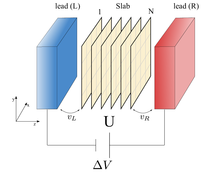
Figure 1: (Color online) Sketch of the correlated slab sandwiched between semi-infinite metallic leads. $v_{L}$ and $v_{R}$ represent respecitvely left and right slab-leads hybridization coupling.

A finite bias $\Delta V$ across the system is applied by coupling with an external environment composed by two, left ($L$) and right ($R$), semi-infinite metallic leads described by not interacting Hamiltonians with symmetrically shifted energy bands

$$H_{\text{Lead}}=\sum_{\alpha=L,R}\;\sum_{\mathbf{k},k_{\perp},\sigma}\big{(}\varepsilon^{\alpha}_{\mathbf{k}}+t^{\alpha}_{k_{\perp}}-\mu_{\alpha}\big{)}\,c^{\dagger}_{\mathbf{k}k_{\perp}\alpha\sigma}c^{\phantom{\dagger}}_{\mathbf{k}k_{\perp}\alpha\sigma},$$ (2)

where $k_{\perp}$ labels the $z-$component of the electron momentum. In Eq. (2) $\varepsilon^{\alpha}_{\mathbf{k}}=-2t_{\alpha}\big{(}\cos k_{x}+\cos k_{y}\big{)}$, $t^{\alpha}_{k_{\perp}}=-2t_{\alpha}\,\cos k_{\perp}$, where we shall assume $t_{L}=t_{R}=t$, and $\mu_{L/R}=\pm e\Delta V/2$, with $e$ the electron charge. We couple the system to the metallic leads through a finite tunneling amplitude between the left(right) lead and the first(last) layer, i.e.

$$H_{\text{Hyb}}=\sum_{\alpha=L,R}\sum_{\mathbf{k},k_{\perp},\sigma}\Big{(}v^{\alpha}_{k_{\perp}}\,c^{\dagger}_{\mathbf{k}k_{\perp}\alpha\sigma}d^{\phantom{\dagger}}_{\mathbf{k}z_{\alpha}\sigma}+H.c.\Big{)},$$ (3)

where $z_{L}=1$, $z_{R}=N$ and

$$v^{\alpha}_{k_{\perp}}=\sqrt{\frac{2}{N_{\perp}}}\;\sin k_{\perp}\,v_{\alpha},$$ (4)

which corresponds to open boundary conditions for the leads along the $z-$direction.

The final Hamiltonian is thus the sum of Eqs. (1), (2) and (3)

$$H=H_{\text{Slab}}+H_{\text{Leads}}+H_{\text{Hyb}}.$$ (5)

We drive the system out-of-equilibrium by suddenly switching the tunneling between the slab and the leads, that is $v_{L}(t)=v_{R}(t)=v_{\text{hyb}}\,\theta(t)$, and by turning on a finite bias $\Delta V(t)=\Delta V\,r(t)$ according to a time-dependent protocol $r(t)$ that, if not explicitly stated, we also take as a step function. We exploit the local energies $E_{z}$ in Eq. (1) to model the potential drop between left and right leads. Even though the profile of the inner potential should be self-consistently determined by the long range coulomb interaction, see e.g. Refs. Charlebois et al., 2013 and Chen and Freericks, 2007, we assume that a flat profile $E_{z}=0$ represents a reasonable choice for the system in its metallic phase, simulating the screening of the electric field inside the metal. On the other hand, in the insulating phase we shall assume a linear potential drop $E_{z}=e\Delta V(N+1-2z)/2(N+1)$ matching the left and right leads chemical potential for $z=0$ and $z=N+1$. In the rest of the work we will assume the units $e=1$ and $\hbar=1$.

Since an exact solution of the time-dependent Schrödinger equation for the model (5) is not feasible we resort the so called time-dependent Gutzwiller approximation Schiró and Fabrizio (2010) and its extension to inhomogeneous systems. André et al. (2012) While we refer the reader to Ref. Fabrizio, 2013 for a detailed derivation, we sketch the main steps that lead to the Gutzwiller dynamical equations for the present case of an inhomogeneous system coupled to semi-infinite leads.

As customary we split the Hamiltonian (5), $H=\mathcal{H}_{0}+\mathcal{H}_{loc}$, into a not-interacting term $\mathcal{H}_{0}$ and a purely local interaction part $\mathcal{H}_{loc}$

$$\begin{split}\mathcal{H}_{0}&=H_{\text{leads}}+H_{\text{hyb}}+\sum_{z=1}^{N}\sum_{\mathbf{k},\sigma}\epsilon_{\mathbf{k}}\,d^{\dagger}_{\mathbf{k},z,\sigma}d^{\phantom{\dagger}}_{\mathbf{k},z,\sigma}\\ &\phantom{=}+\sum_{z=1}^{N-1}\sum_{\mathbf{k},\sigma}\Big{(}t_{z,z+1}\,d^{\dagger}_{\mathbf{k},z+1,\sigma}d^{\phantom{\dagger}}_{\mathbf{k},z,\sigma}+H.c.\Big{)},\end{split}$$ (6)

$$\mathcal{H}_{loc}=\sum_{z=1}^{N}\sum_{\mathbf{r}}\,\frac{U}{2}\big{(}n_{\mathbf{r},z}-1\big{)}^{2}+E_{z}n_{\mathbf{r},z}\equiv\sum_{\mathbf{R}}\,\mathcal{H}_{loc,\mathbf{R}},$$ (7)

where $\mathbf{R}=(\mathbf{r},z)$, and define the time-dependent variational wavefunction

$$|{\Psi(t)}\rangle=\prod_{\mathbf{R}}\mathcal{P}_{\mathbf{R}}(t)|{\Psi_{0}(t)}\rangle,$$ (8)

where $|{\Psi_{0}(t)}\rangle$ is a time-dependent wavefunction for which Wick theorem holds, and $\mathcal{P}_{\mathbf{R}}$ are linear operators that act on the local Hilbert space at site $\mathbf{R}$ and control, through a set of time-dependent variational parameters, the weights of the local electronic configurations. The dynamics of the variational parameters and of the wavefunction $|{\Psi_{0}(t)}\rangle$ is obtained by applying the time-dependent variational principle $\delta\mathcal{S}=0$ on the action $\mathcal{S}=\int\,\langle{\Psi}|{\,i\partial_{t}-H\,}|{\Psi}\rangle$. Upon imposing the following constraints

$$\begin{split}&\langle{\Psi_{0}(t)}|{\,\mathcal{P}^{{\dagger}}_{\mathbf{R}}(t)\mathcal{P}_{\mathbf{R}}(t)\,}|{\Psi_{0}(t)}\rangle=1,\\ &\langle{\Psi_{0}(t)}|{\,\mathcal{P}^{{\dagger}}_{\mathbf{R}}(t)\mathcal{P}_{\mathbf{R}}(t)\,d^{\dagger}_{\mathbf{R}\sigma}d^{\phantom{\dagger}}_{\mathbf{R}\sigma^{\prime}}\,}|{\Psi_{0}(t)}\rangle\\ &\qquad\qquad\qquad=\langle{\Psi_{0}(t)}|{\,d^{\dagger}_{\mathbf{R}\sigma}d^{\phantom{\dagger}}_{\mathbf{R}\sigma^{\prime}}\,}|{\Psi_{0}(t)}\rangle,\end{split}$$ (9)

expectation values can be analytically computed in lattices with infinite coordination number. Fabrizio (2013) In particular, if one parametrizes the Gutzwiller operators $\mathcal{P}_{\mathbf{R}}$ through site- and time-dependent variational matrices $\hat{\Phi}_{\mathbf{R}}(t)$ in the basis of the local electronic configurations, the following closed set of coupled dynamical equations are readily obtained Fabrizio (2013)

$$i\,\frac{\partial\mid\Psi_{0}(t)\rangle}{\partial t} = \mathcal{H}_{*}[\hat{\Phi}(t)]\mid\Psi_{0}(t)\rangle,$$ (10)

$$i\frac{\partial\hat{\Phi}_{\mathbf{R}}(t)}{\partial t} = \mathcal{H}_{loc,\mathbf{R}}\hat{\Phi}_{\mathbf{R}}(t)$$ (11)

$$+\langle\Psi_{0}(t)\mid\frac{\partial\mathcal{H}_{*}[\hat{\Phi}(t)]}{\partial\hat{\Phi}_{\mathbf{R}}^{{\dagger}}(t)}\mid\Psi_{0}(t)\rangle.$$

In Eqs. (10) and (11) $\mathcal{H_{*}}[\hat{\Phi}(t)]$ is an effective not-interacting Hamiltonian that depends parametrically on the variational matrices $\hat{\Phi}_{\mathbf{R}}(t)$. Eq. (10) represents an effective Schrödinger equation for non-interacting electrons and is commonly interpreted as a Hamiltonian for the coherent quasiparticles. The dynamics of the local variational parameters determined by Eq. (11) can be associated to the incoherent excitations of the Hubbard bands. The two dynamical evolutions are coupled in a mean-field like fashion, each degree of freedom providing a time-dependent field for the other one. This aspect, although being an approximation that does not allow to reproduce a genuine relaxation to a steady state, still represents a great advantage of the present method with respect to the standard time-dependent Hartree-Fock.

If we use as local basis at site $\mathbf{R}$ the empty state $|{0}\rangle$, the doubly-occupied one, $|{2}\rangle$, and the singly-occupied ones, $|{\sigma}\rangle$ with $\sigma=\uparrow,\downarrow$ referring to the electron spin, and discard magnetism and $s$-wave superconductivity, the matrix $\hat{\Phi}_{\mathbf{R}}(t)$ can be chosen diagonal with matrix elements $\Phi_{\mathbf{R},00}(t)\equiv\Phi_{\mathbf{R},0}(t)$, $\Phi_{\mathbf{R},22}(t)\equiv\Phi_{\mathbf{R},2}(t)$, and $\Phi_{\mathbf{R},\uparrow\uparrow}(t)=\Phi_{\mathbf{R},\downarrow\downarrow}(t)\equiv\Phi_{\mathbf{R},1}(t)/\sqrt{2}$. Due to translational invariance within each $xy$ plane, the variational matrices depend explicitly only on the layer index $z$, i.e. $\hat{\Phi}_{\mathbf{R}}(t)=\hat{\Phi}_{z}(t)$, and the constraints (9) are satisfied by imposing

$$\left|\Phi_{z,0}(t)\right|^{2}+\left|\Phi_{z,2}(t)\right|^{2}+\left|\Phi_{z,1}(t)\right|^{2}=1,$$ (12)

and

$$\begin{split}\delta_{z}(t)&\equiv\left|\Phi_{z,0}(t)\right|^{2}-\left|\Phi_{z,2}(t)\right|^{2}\\ &=1-\sum_{\mathbf{k}\sigma}\,\langle{\Psi_{0}(t)}|{\,d^{\dagger}_{\mathbf{k}z\sigma}d^{\phantom{\dagger}}_{\mathbf{k}z\sigma}\,}|{\Psi_{0}(t)}\rangle,\end{split}$$ (13)

where $\delta_{z}(t)$ is the instantaneous doping of layer $z$. Through this choice we obtain the following effective Hamiltonian $\mathcal{H}_{*}[\hat{\Phi}(t)]$

$$\begin{split}\mathcal{H}_{*}[\hat{\Phi}(t)]&=H_{\text{Leads}}+\sum_{z=1}^{N}\sum_{\mathbf{k},\sigma}\left|R_{z}(t)\right|^{2}\epsilon_{\mathbf{k}}\,d^{\dagger}_{\mathbf{k},z,\sigma}d^{\phantom{\dagger}}_{\mathbf{k},z,\sigma}\\ &+\sum_{z=1}^{N-1}\sum_{\mathbf{k},\sigma}\,\Big{(}R^{*}_{z+1}(t)\,R_{z}(t)\;d^{\dagger}_{\mathbf{k},z+1,\sigma}d^{\phantom{\dagger}}_{\mathbf{k},z,\sigma}+H.c.\Big{)}\\ &+\sum_{\alpha=L,R}\,\sum_{\mathbf{k},k_{\perp},\sigma}\Big{(}v_{k_{\perp}}\,R_{z_{\alpha}}(t)\;c^{\dagger}_{\mathbf{k}k_{\perp}\alpha\sigma}d^{\phantom{\dagger}}_{\mathbf{k}z_{\alpha}\sigma}+H.c.\Big{)},\end{split}$$ (14)

where the layer-dependent hopping renormalization factor reads

$$R_{z}(t)=\sqrt{\frac{\displaystyle 2}{\displaystyle 1-\delta_{z}(t)^{2}}}\;\bigg{(}\Phi_{z,0}(t)\Phi^{*}_{z,1}(t)+\Phi_{z,2}^{*}(t)\Phi_{z,1}(t)\bigg{)}.$$ (15)

Straightforward differentiation of Eq. (14) with respect to $\hat{\Phi}^{{\dagger}}_{z}(t)$ yields the equations of motion for the variational matrices (11), which together with the effective Schrödinger equation (10) completely determine the variational dynamics within the TDG approximation. Though the derivation of the set of coupled dynamical equations is very simple, the final result is cumbersome so that we present it in the appendix A together with details on its numerical integration.

We characterize the non equilibrium behavior of the system by studying the electronic transport through the slab. In particular, in the following we shall define the electronic current flowing from the left/right lead to the first/last layer of the slab as the contact current with expression

$$j_{\alpha}(t)=-i\left[\sum_{\mathbf{k}\sigma}\sum_{k_{\perp}}v_{k_{\perp}}\langle{\Psi(t)}|{\,d^{\dagger}_{\mathbf{k}z\sigma}c^{\phantom{\dagger}}_{\mathbf{k}k_{\perp}\alpha\sigma}\,}|{\Psi(t)}\rangle-c.c.\right],$$ (16)

and the layer current as the current flowing from the $z$-th to the $z+1$-th layer, i.e.

$$j_{z}(t)=-i\left[\sum_{\mathbf{k}\sigma}\langle{\Psi(t)}|{d^{\dagger}_{\mathbf{k}z\sigma}d^{\phantom{\dagger}}_{\mathbf{k}z+1\sigma}}|{\Psi(t)}\rangle-c.c.\right].$$ (17)

Within the TDG approximation these two observables read, respectively,

$$j_{\alpha}(t)=-i\bigg{[}R_{z_{\alpha}}^{*}(t)\sum_{\mathbf{k}\sigma}\sum_{k_{\perp}}v_{k_{\perp}}\langle{d^{\dagger}_{\mathbf{k}z\sigma}c^{\phantom{\dagger}}_{\mathbf{k}k_{\perp}\alpha\sigma}}\rangle-c.c.\bigg{]}$$ (18)

and

$$j_{z}(t)=-i\bigg{[}R_{z}^{*}(t)R_{z+1}(t)\sum_{\mathbf{k}\sigma}\langle{d^{\dagger}_{\mathbf{k}z\sigma}d^{\phantom{\dagger}}_{\mathbf{k}z+1\sigma}}\rangle-c.c.\bigg{]},$$ (19)

where $\langle{\ldots}\rangle\equiv\langle{\Psi_{0}(t)}|{\ldots}|{\Psi_{0}(t)}\rangle$. Notice that, due to the left/right symmetry, $j_{L}=-j_{R}$ and we need only to consider currents for $z\leq N/2$.

II Non-equilibrium transport in the strongly correlated metal

In this section we consider the case of a correlated slab in its metallic phase, $U\!<\!U_{c}$ where $U_{c}\!\approx\!16$ is the critical value above which the system is Mott insulating in equilibrium.

II.1 Zero-bias dynamics

To start with we shall consider the dynamics at zero-bias $\Delta V\!=\!0$. In this case we assume that the non-equilibrium perturbation is the sudden switch of the tunnel amplitude $v_{\text{\tiny hyb}}$ between the correlated slab and the leads. In the equilibrium regime, the metallic character at the un-contacted surfaces is strongly suppressed with respect to the bulk as effect of the reduced kinetic energy. This suppression, commonly described in terms of a surface dead layer, extends over a distance which is quite remarkably controlled by a critical correlation length $\xi$ associated to the Mott transition. Indeed $\xi$ is found to grow approaching the metal-insulator transition and diverges at the transition point. Borghi et al. (2009) In presence of a contact with external metallic leads the surface state is characterized by a larger quasiparticle weight with respect to that of the bulk irrespective of its metallic or insulating character, realizing what is called a living layer. Borghi et al. (2010) As we shall see in the following, by switching on $v_{\text{\tiny hyb}}$ it should be possible to turn the dead layer into the living one on a characteristic time scale $\tau$: The dynamical counterpart of the correlation length $\xi$.

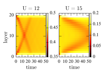
Figure 2: (Color online) Layer-resolved dynamics of the local quasiparticle weights $|R_{z}(t)|^{2}$ for a slab of $N=20$ layers and two values of the interaction $U$. The slab-lead hybridization is equal to the inter-layer hopping amplitude $v_{\text{\tiny hyb}}=1.0$.

In Fig. 2 we show the time-evolution of the layer-dependent quasiparticle weight $Z_{z}(t)\!\equiv\!\left|R_{z}(t)\right|^{2}$ for a $N\!=\!20$ slab and different values of the interaction $U$. The dynamics shows a characteristic light-cone effect, i.e. a constant velocity propagation of the perturbation from the junctions at the external layers $z\!=\!1$ and $z\!=\!N$ to the center of the slab. After few reflections the light-cone disappears leaving the system in a stationary state. The velocity of the propagation is found to be proportional to the bulk quasiparticle weight hence it decreases as the Mott transition is approached for $U\!\rightarrow\!U_{c}$.

The boundary layers are strongly perturbed by the sudden switch of the tunneling amplitude. In particular, we observe in Fig. 3(a) that the surface dead layers rapidly transform into living layers with stationary quasiparticle weights greater than the bulk ones and equal to the equilibrium values for the same set-up. Borghi et al. (2010) This has to be expected since the energy injected is not extensive. On the contrary, the bulk layers are weakly affected by the coupling with the metal leads, see Fig. 3(b). Their dynamics is only affected by small oscillations and temporary deviations from the stationary values due to the perturbation propagation described by the light-cone reflections.

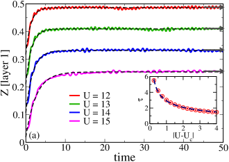
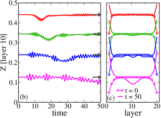
Figure 3: (Color online) (a) Dynamics of the local quasiparticle weight for the first layer. Dashed lines are the fitting curves obtained with Eq. (20). Arrows represent the hybridized slab equilibrium values. Inset: dead layer awakening time as a function of $U$. Dashed lines represents the fitting curve $\tau=\alpha/|U-U_{c}|^{\nu_{*}}$ with $\nu_{*}\approx 0.4895$ (b) Dynamics of the local quasiparticle weight for the bulk ($z=10$) layer. Arrows represent the hybridized slab equilibrium values. (c) Quasiparticle weight profiles at times $t=0$ (dotted lines) and $t=50$ (lines).

We characterize the evolution from the dead to the living layer by fitting the dynamics of the boundary layer quasiparticle weight with an exponential relaxation towards a stationary value:

$$Z(t)=Z_{\text{dead}}+\Big{(}Z_{\text{living}}-Z_{\text{dead}}\Big{)}\,\Big{(}1-e^{-t/\tau}\Big{)}.$$ (20)

As illustrated in Fig. 3(b) the dynamics shows a slowing-down upon approaching the Mott transition. In particular the dead-layer wake-up time $\tau$ diverges as $\tau\!\sim\!|U\!-\!U_{c}|^{-\nu_{*}}$ when we approach the critical value $U_{c}$ with a critical exponenent that we estimate as $\nu_{*}\!=\!0.4895$, very close to the mean-field value $\nu_{*}\!=\!1/2$. Such a mean-field dependence, similar to that of the correlation lenght $\xi\!\sim\!|U\!-\!U_{c}|^{-1/2}$  Borghi et al. (2010) implies, through $\tau\sim\xi^{\,\zeta}$, a dynamical critical exponent $\zeta\!=\!1$.

II.2 Small-bias regime

We shall now focus on the the dynamics in the presence of an applied bias. In the Fig. 4 we report our results for the real-time dynamics of the currents at the contacts and layers, defined by Eqs. (19)–(18), after a sudden switch of the bias $\Delta V$ and a flat inner potential.

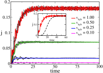
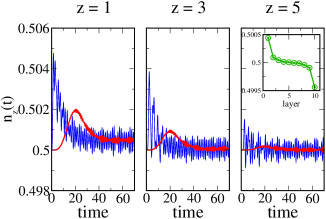
Figure 4: (Color online) Top: Real-time dynamics of the currents computed at the slab-lead contact (thick lines) and between two neighboring layers (light grey lines) after a bias quench with $\Delta V=0.5$ and $U=12$. for a $N=10$ slab and different values of the slab-leads coupling $v_{\text{\tiny hyb}}$. Inset: Current dynamics for a ramp-like switching protocol $r(t)=[1-3/2\cos(\pi t/\tau_{*})+1/2\cos(\pi t/\tau_{*})^{3}]/4$ compared to the sudden quench limit ($\tau_{*}=30$). Bottom: Dynamics of the local electronic densities $n_{z}(t)$ for the $1^{\text{st}}$, $3^{\text{rd}}$ and $5^{\text{th}}$ layer and $v_{\text{\tiny hyb}}=1.0$. Inset: stationary density profile showing an almost flat density distribution with slighlty doped regions near the left and right contacts.

We observe that the contact and the layer currents display very similar dynamics, characterized by a monotonic increase at early times and a saturation to stationary values at longer times. The stationary dynamics displays small undamped oscillations around the mean value due to oscillations of the layer-dependent electronic densities (see Fig. 4(b)). As we already mentioned, the persistence of oscillations, i.e.the absence of a true relaxation to a steady-state, is a characteristic of the essentially mean-field nature of the method. However, this problem can be overcome either by time-averaging the signal or, as shown in the inset of Fig. 4, using a finite-time switching protocol $r(t)$ for the voltage bias. In both cases we end up with the same currents and density profiles, which result almost flat as a function of the layer, as expected in the metallic case.

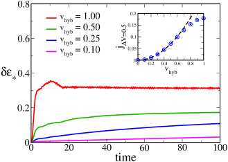
Figure 5: (Color online) Relative variation of the slab internal energy as defined in Eq. 21 for the same set of parameters of Fig. 4. Inset: Stationary current for $\Delta V=0.5$ as a function of the hybridization with the leads with a fitting curve $j(v_{\text{\tiny hyb}})=j_{0}\,v_{\text{\tiny hyb}}^{2}$ (dashed line).

We highlight that the non-equilibrium dynamics is strongly dependent on the coupling between the system (correlated slab) and the external environment (leads), represented in this case by the slab-lead tunneling amplitude $v_{\text{\tiny hyb}}$. This is evident from the stationary value of the current that increases as a function of $v_{\text{\tiny hyb}}$, as expected since this latter sets the rate of electrons/holes injection from the leads into the slab. Furthermore, the coupling to an external environment is essential to redistribute the energy injected into the system after a sudden perturbation so to lead to a final steady state characterized by a stationary value of the internal energy. In order to study the competition between energy dissipation and energy injection rate we plot, in Fig. 5, the time-dependence of the relative variation of the slab internal energy with respect to its equilibrium value:

$$\delta\epsilon_{*}(t)\equiv\frac{E_{*}(t)-E_{*}(t=0)}{\left|E_{*}(t=0)\right|},$$ (21)

where

$$\begin{split}E_{*}(t)\equiv&\langle{\Psi(t)}|{H_{\text{Slab}}}|{\Psi(t)}\rangle\approx\langle{\Psi_{0}(t)}|{\mathcal{H}_{*}\big{[}\hat{\Phi}(t)\big{]}}|{\Psi_{0}(t)}\rangle\\ &+\sum_{z}\mathrm{Tr}\left(\hat{\Phi}_{z}(t)^{{\dagger}}\mathcal{H}_{loc,z}\hat{\Phi}_{z}(t)\right).\end{split}$$

The last expression holds within the TDG approximation. We observe the existence of two regimes as a function of the coupling to the leads $v_{\text{\tiny hyb}}$. When the system is weakly coupled to the external environment the energy shows an almost linear increase in time without ever reaching any stationary value. This signals that the dissipation mechanism is not effective on the scale of the simulation time. For larger values of $v_{\text{\tiny hyb}}$, the dissipation mechanism becomes more effective. The internal energy shows a faster growth at initial times, due to the larger value of the current setting up through the system. Further increasing (see the case $v_{\text{\tiny hyb}}\!=\!1.0$ in the figure) the initial fast rise is of the energhy is followed by a downturn towards a stationary value, which in turn is reached very rapidly. As shown in the inset of Fig. 5 the crossover between the non-dissipative and dissipative regimes coincides with the point in which the current deviates from linear-response theory – which predicts a quadratically increasing current $j\!\propto\!v_{\text{\tiny hyb}}^{2}$– and bends towards smaller value.

II.3 Large-bias regime

The interplay between the energy injection and the dissipation highlighted in the dynamics of the slab internal energy (Fig. 5) is a direct consequence of the fact that in our model these two mechanisms are controlled by the coupling with the same external environment. Therefore, we may envisage a situation in which the internal energy of the slab grows so fast that the leads are unable to dissipate the injected energy preventing a stationary current to set in. This phenomenon occurs at large values of the voltage bias ($\Delta V\!\gtrsim\!1$) and of the tunneling amplitude $v_{\text{\tiny hyb}}$, i.e.when the slab is rapidly kicked away from equilibrium. In order to illustrate this point we report in Fig. 6 the current dynamics for the same parameters as in the previous Fig. 4 but for larger value of the voltage bias $\Delta V\!=\!2.0$. We observe that, while for weak tunneling ($v_{\text{\tiny hyb}}\!=\!0.1$) the current flows to a steady state, upon increasing $v_{\text{\tiny hyb}}$ the stationary state can not be reached and strong chaotic oscillations characterize the long-time evolution.

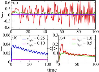
Figure 6: (Color online) (a) Real-time dynamics for the contact currents for the same parameters and values of hybridization coupling of Fig. 4 and $\Delta V=2.0$. (b) Blow-up of the currents dynamics for $v_{\text{\tiny hyb}}=0.1$ and $v_{\text{\tiny hyb}}=0.25$. (c) Dynamics of the current time average $\langle{j(t)}\rangle$ as defined in the main text for $v_{\text{\tiny hyb}}=0.5$ and $v_{\text{\tiny hyb}}=1.0$.

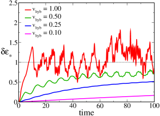
Figure 7: (Color online) Dynamics of the relative energy variation for the same parameters in Fig. 6.

Indeed, the inability of reaching a steady-state is intertwined with the fast increase of the slab internal energy, as revealed by our results in Fig. 7. In particular, for $v_{\text{\tiny hyb}}\!=\!1.0$ the relative variation of the internal energy rapidly reaches $\delta\epsilon_{*}(t)\!\approx\!1$, after which it starts to oscillate chaotically just like the currents does. The same behavior shows up in the dynamics of the quasiparticle weight averaged over all layers:

$$Z_{*}(t)\equiv\frac{1}{N}\sum_{z=1}^{N}Z_{z}(t)=\frac{1}{N}\sum_{z=1}^{N}\left|R_{z}(t)\right|^{2},$$ (22)

which displays fast and large oscillations whereas it is smooth in the case of small $v_{\text{\tiny hyb}}$ (see Fig. 8).

This behavior is similar to that observed across the dynamical phase-transition in the half-filled Hubbard model after an interaction quench Schiró and Fabrizio (2010); Eckstein et al. (2009) occurring when the injected energy exceeds a threshold.Sandri et al. (2012); Mazza and Fabrizio (2012) This correspondence is further supported by noting that the onset of chaotic behavior occurs precisely when the internal energy $E_{*}(t)$ of the slab reaches zero (see Fig. 9). The value $E_{*}\!=\!0$ is indeed the energy of a Mott insulating wavefunction within the Gutzwiller approximation. This anomalous behavior thus suggests that as soon as the energy crosses zero $E_{*}(t)\!\geq\!0$ the system gets trapped into an insulating state characterized by a strongly suppressed tunneling into the metal. This prevents the excess energy to flow back into the leads and does not allow for the relaxation to a metal with a steady current.

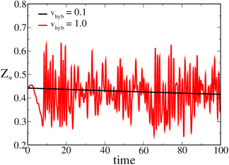
Figure 8: (Color online) Dynamics of the mean quasiparticle weight for the same parameters in Fig. 6 and $v_{\text{\tiny hyb}}=0.1$ (black line) and $v_{\text{\tiny hyb}}=1.0$ (red line).

We associate this behavior to a shortcoming of the TDG approximation, does not include all the dissipative processes and therefore artificially enhances the stability of such a metastable state. If we want to compare this behavior with a real system, we can argue that the TDG description only describes a transient state produced by the large initial heating of the slab that is temporarily pushed into a high-temperature incoherent phase of the Hubbard model, which takes a long time to equilibrate back with the metal leads but evidently not the infinite time that the TDG approximation suggests. This behavior is similar to what has been observed by DMFT in the case of an homogeneous system driven by a static electric field in the absence of external dissipative channels. Amaricci et al. (2012).

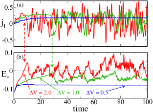
Figure 9: (Color online) Current (a) and internal energy dynamics (b) for $U=12$, $v_{\text{\tiny hyb}}\!=\!1.0$ and three values of the applied bias. The occourence of the breakdown of the stationary dynamics due to the dynamical transition is highlighted by the vertical arrows.

In the case of an interaction quench it was found that, even though the absence of a true exponential relaxation is faulty, the time-averaged values of observables as obtained within the TDG approximation might still be representative of the true dynamics.Schiró and Fabrizio (2010); Sandri et al. (2012) This allows us to define a sensible current by time averaging the real-time evolution, i.e.through

$$\langle{j(t)}\rangle=\frac{1}{t}\int_{0}^{t}d\tau j(\tau),$$ (23)

which indeed approaches a finite value at long enough times (see Fig. 6(c)).

II.4 Current-bias characteristics

The overall picture emerging from our investigation of the metallic case can be summarized by an inspection of the evolution of the current as a function of the bias (current-bias characterisctic) for different values of the interaction strength.

In the limit of weak coupling to the external environment, we have seen that the currents display a stationary dynamics in a wide range of bias values. In Fig. 10 we report these stationary values as a function of the bias for $v_{\text{\tiny hyb}}\!=\!0.1$ and a wide range of interaction strenghts.

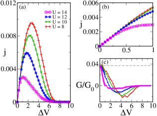
Figure 10: (Color online) (a): current-bias characteristics for a $N=10$ slab for different values of $U$ and $v_{\text{\tiny hyb}}=0.1$. (b) blow-up of the linear part of the current-bias characteristics. (c): Differential conductance measured respect to the quantum conductance $G_{0}=1/2\pi$ in our units. Grey line represents the universal zero-bias value.

All the curves show a crossover between a linear regime at small bias and a monotonic decrease for larger values. This behavior is similar to what was already observed in different contexts. Amaricci et al. (2012); Aron et al. (2012); Mierzejewski et al. (2011); Arrigoni et al. (2013) We connect the drop of the current for large biases to the reduction of energy overlap between the leads and the slab electronic states at large bias. In the linear regime we find that the zero-bias differential conductance $G(0)\!=\!\left.\partial j/\partial\Delta V\right|_{\Delta V=0}$ is universal with respect to the interaction strength Lanatà (2010); Li et al. (2014) as expected when the electronic transport is determined only by the low-energy quasiparticle excitations.

Within the TDG approximation this fact can be easily rationalized by noting that quasiparticles are controlled by the non-interacting Hamiltonian $\mathcal{H}_{*}$ in Eq. (14), characterized by a hopping amplitude renormalized by the factors $|R|\!\leq\!1$. This leads to an enhancement of the quasiparticle density of states by a factor $\nu\!\sim\!1/|R|^{2}$ that at low bias compensates the reduction of tunneling rate into the leads. Conversely, as the bias increases the current-bias characteristics starts deviating from the universal low-bias behavior and becomes strongly dependent on the interaction strenght $U$. Li et al. (2014) In particular, the crossover between the positive and the negative differential conductance regimes gets shifted towards smaller values of the bias as $U$ is increased as effect of the shrinking of the coherent quasiparticle density of states.

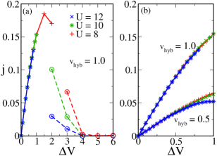
Figure 11: (Color online) Left: current-bias characteristics for a $N=10$ slab, different values of $U$ and $v_{\text{\tiny hyb}}=1.0$. Plus, cross and star symbols represents stationary currents values, while circles represent converged currents time averages values. Right: blow-up of the linear part of the current-bias characteristics for $v_{\text{\tiny hyb}}=0.5$ and $v_{\text{\tiny hyb}}=1.0$, showing universal zero-bias conductivity $G/G_{0}\approx 0.452$ and $1.203$ respectively.

As discussed in the previous section, increasing the coupling to the external environment leads to a chaotic regime at large bias, in a regime where we cannot identify anymore a stationary current. However, as mentioned above, we can still extract a meaningful estimate of the current through its time-average Eq. (23)), restricting to the range of bias for which the latter is well converged. This is explicitely illustrated in Fig. 11 for the current-bias characteristics at $v_{\text{\tiny hyb}}\!=\!1.0$. The open circles represent currents computed using converged time averaged while the other symbols represent currents characterized by a stationary dynamics. Our results show that the curves have qualitatively the same features of the small $v_{\text{\tiny hyb}}$ case with a universal linear conductance and a crossover to a negative conductance regime.

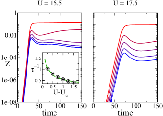
Figure 12: (Color online) Real-time dynamics for the quasiparticle weights from layer $1$ to $5$ (from top to bottom) of a $N=10$ Mott insulating slab suddenly coupled to the metallic leads ($v_{\text{hyb}}=1.0$). $U=16.5$ and $U=17.5$. Inset: inverse of the characteristic time for the exponential quasiparticle formation $\tau^{-1}\sim(U-U_{c})^{-\nu_{*}}$, $\nu_{*}\approx 0.4753$.

III Dielectric breakdown of the Mott insulating phase

We now move the discussion to the effect of an applied voltage bias to a slab which is in a Mott insulating regime because $U>U_{c}$. Unlike the metallic case, we now assume that the field penetrates inside the slab, leading to a linear potential profile of the form $E_{z}=\Delta V(N+1-2z)/2(N+1)$ matching the chemical potential of the left and right leads for $z=0$ and $z=N+1$ respectively.

III.1 Evanescent bulk quasiparticle

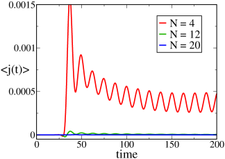
Figure 13: (Color online) Time-averaged currents for three slabs with applied bias $\Delta V=0.5$. $U=16.5>U_{c}$, $v_{\text{\tiny hyb}}=1.0$ and $N=4,12,20$ (from top to bottom).

Within the Gutzwiller approximation the Mott insulator is characterized by a vanishing number of doubly occupied and empty sites as well as by a zero renormalization factor $R\!=\!0$, leading to a trivial state with zero energy. However, it has been shown that in the presence of the metallic leads evanescent quasiparticles  Borghi et al. (2010); Zenia et al. (2009) appear inside the insulating slab. This is revealed by a finite quasiparticle weight which is maximum at the leads and decays exponentially in the bulk of the slab with a characteristic length $\xi\sim(U-U_{c})^{-1/2}$ which defines the critical correlation length of the Mott transition. Borghi et al. (2010)

In Fig. 12 we show the dynamics of the formation of evanescent quasiparticles after the sudden switch on of the coupling to the leads $v_{\text{\tiny hyb}}$. We observe a rapid increase of the quasiparticle weight as soon as the coupling is switched on. The rapid increase can be reasonably well parameterized as an exponential with a characteristic growth time $\tau$. The results for $\tau^{-1}$ reported in the inset of the left panel of Fig. 12) clearly show that the increase of the quasiparticle weight becomes faster as the Mott transition is approached. Interestingly, the exponential growth is not limited to the boundary layers close to the leads, but it is present throughout the slab, with a characteristic time $\tau(z)$ which is nearly uniform in space.

Such an exponential growth is suggestive of an avalanche effect, driven by the combined action of the high-energy excitations (Hubbard bands) and of the quasiparticles, which within the Gutzwiller approach can be associated to the variational parameters $\Phi_{z,n}(t)$ and to the non-interacting Slater determinant $\mid\!\Psi_{0}(t)\rangle$, respectively.

As outlined in Appendix B.1, we can reproduce the long-time approach to the steady state corresponding to evanescent quasiparticles at equilibrium, considering a simplified dynamics in which we neglect the dynamics of the Slater determinant $\mid\!\Psi_{0}(t)\rangle$ and take into account only that of $\Phi_{z,n}(t)$. The latter can be analytically written in terms of a Klein-Gordon-like equation for the hopping renormalization factors $R(z,t)$

$$\frac{\displaystyle 1}{\displaystyle c^{2}}\,\ddot{R}(z,t)-\nabla^{2}\,R(z,t)+m^{2}\,c^{2}\,R(z,t)=0,$$ (24)

with parameters (see Appendix B.1):

$$c^{2}=\frac{\displaystyle U}{\displaystyle 24},\qquad m^{2}c^{2}=6(U-1)=\xi^{-2}.$$ (25)

As anticipated above the simplified dynamics described by Eq. 24 correctly captures the long-time behaviour of the system, but it can not reproduce the short time exponential growth. In the latter regime the time evolution is indeed governed by the interplay between Hubbard bands and quasiparticles, responsible for the evenescent quasiparticle formation into the Mott insulating slab, which is neglected in the approximation leading to Eq. 24.

The presence of the evanescent bulk quasiparticle provides a conducting channel accross the slab, possibly leading to finite currents upon the application of a finite bias. In particular, we expect that if the slab lenght smaller than the decay length $\xi$ every finite bias $\Delta V$ is sufficient to induce a finite current through the slab. On the other hand we expect the current to be suppressed when the slab is longer than $\xi$ This is confirmed by the results reported in Fig. 13 where we show the average current for a bias $\Delta V=0.5$, in the linear regime in the metallic case, and different slab sizes $N$. A finite current is rapidly injected for small $N\!=\!4$, whereas it does not for larger systems (e.g. $N\!=\!12$ or $N\!=\!20$).

III.2 Dielectric breakdown currents

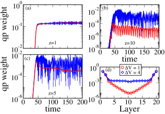
Figure 14: (Color online) Layer dependent quasiparticle weight dynamics for layers 1 (a), 5(b) and 10(c) of a $N=20$ slab, $U=16.5$, $v_{\text{\tiny hyb}}=1.0$ and two values of the applied bias $\Delta V=1.0$(red lines) and $\Delta V=4.0$ (blue lines). (d): time-averaged stationary quasiparticle weight profile.

Increasing the value of the applied bias we observe an enhancement of the quasiparticle weight throughout the slab. This effect is illustrated in Fig. 14 where panels (a-c) show the the dynamics of the quasiparticle weights in a driven Mott insulating slab with different values of the bias for three different layers ($z=1,5,10$). While the dynamics is characterized by strong oscillations reminescent of the inchoerent dynamics discussed in Sec. II for the metallic slab under a large applied bias, the time-averaged quantities in the long-time limit converge to stationary values. The spatial distribution as a function of the layer index shows a strong enhancement in the bulk upon increasing the bias (Fig. 14d).

Such enhancement results in a finite current flowing. Indeed, as shown in Fig. 15, the time-averaged current has a damped oscillatory behavior that converges towards a steady value, although the real-dynamics follows a seemingly chaotic pattern (see the inset). We extract the stationary values by fitting the current time-averages with:

$$\langle{j(t)}\rangle=j_{\text{steady}}+\frac{\alpha}{t}.$$ (26)

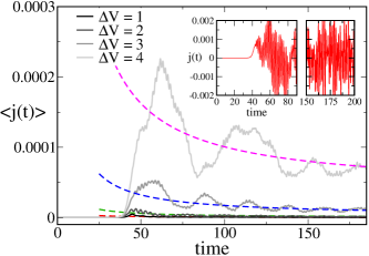
Figure 15: (Color online) Time-averaged currents for the same parameters in Fig. 14 and $\Delta V=4.0,3.0,2.0$ and $1.0$ (from top to bottom). Dashed lines are fitting curves from Eq. (26). Inset: Real time dynamics of the current for $\Delta V=4.0$.

As evident by looking at the results reported in Fig. 15, the stationary value of the current has a non-linear behavior as a function of the applied bias. This effect can be better appreciated in the next Fig. 16, where we plot the current-voltage characteristics for increasing values of the slab size $N$.

Interestingly, the current displays an exponential activated behavior with a characteristic threshold bias which is well described by

$$j_{\text{steady}}(\Delta V)=\gamma\,\Delta V\,\text{e}^{-\Delta V_{\text{th}}/\Delta V}.$$ (27)

Fitting the data with the above relation we obtain $\Delta V_{\text{th}}\propto N$ (see inset in Fig. 16) so that we can rewrite Eq. (27) as function of the electric field $\Delta V/N$:

$$\frac{\displaystyle j_{\text{steady}}(\Delta V)}{\displaystyle\Delta V}=\gamma\,\text{e}^{-E_{\text{th}}/E},$$ (28)

which introduces a size-independent threshold field $E_{\text{th}}$. This expression is suggestive of a Landau-Zener type of dielectric breakdownOka and Aoki (2005); Oka et al. (2003), similar to the results obtained within DMFT studies of either homogeneous Eckstein et al. (2010) and inhomogeneous systems. Okamoto (2007); Eckstein and Werner (2013)

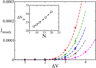
Figure 16: (Color online) Current bias characteristics for $U=16.5$ and different values of the slab lenght $N=8,10,12,16$ and $20$ (from top to bottom). Dashed lines represent fitting curves with Eq. (27). Insets: threshold bias $\Delta V_{th}$ as a function of the slab size.

The Gutzwiller scenario for the dielectric breakdown is further supported by the simple calculation for the stationary regime outlined in the Appendix B, which follows the analysis reported in Ref. Borghi et al., 2010 for the equilibrium case, considering a single metal-Mott insulator interface in the presence of an electrochemical potential $\mu(z)$. As detailed in B, we find that for weak $\mu(z)$, the hopping renormalization factor $R(z)$ satisfies the equation

$$\nabla^{2}R(z)=\Big{(}m^{2}c^{2}-\frac{2\mu(z)^{2}}{c^{2}}\Big{)}\,R(z),$$ (29)

which is nothing but the stationary Klein-Gordon equation (24) in the presence of a field, or alternatively, the Schrœdinger equation of a particle impinging on a potential barrier. For a constant electric field $\mu(z)\!=\!E\,z$ and within the WKB approximation, we obtain the stationary transmission probability beyond the turning point $z_{*}$ of the barrier (see Appendix B):

$$\left|R(z>z_{*})\right|^{2}\sim\exp\left(-\frac{\displaystyle E_{\text{th}}}{\displaystyle E}\right),$$ (30)

where

$$E_{\text{th}}=\frac{\displaystyle\pi}{\displaystyle\sqrt{8}}\;m^{2}\,c^{3}\sim\xi^{-2}.$$ (31)

This calculation identifies the transmission probability (Eq. 30) with the dielectric breakdown currents (Eq. 28) and predicts via the definition of the correlaton lenght (Eq. 25) a threshold electric field increasing with the interaction strenght. Eckstein et al. (2010)

III.3 Quasiparticle energy distribution

Inspired by the evidence that in our description the transport activation is driven by an enhancement of the bulk quasiparticle weight [see Fig. 14(d)] in this section we focus on the spatial distribution of the quasiparticle energy throughout the slab. In order to estimate the time evolution of the quasiparticle energy levels we compute the time-evolution of the layer-dependent chemical potential in the effective non-interacting model Eq. 14, introduced by the coupling to external voltage bias. This quantity can be easily extracted by means of the following unitary transformation of the uncorrelated wavefunction:

$$|{\varphi_{0}(t)}\rangle\!\equiv\!\mathcal{U}(t)\,|{\Psi_{0}(t)}\rangle\,,\;\mathcal{U}(t)\!=\!\prod_{\mathbf{r},z}\exp{\Big{[}i\lambda_{z}(t)\,\hat{n}_{\mathbf{r},z}\Big{]}}$$ (32)

where $\lambda_{z}(t)$ is the time-dependent phase of the hopping renormalization parameters $R_{z}(t)\!\equiv\!\rho_{z}(t)\text{e}^{i\lambda_{z}(t)}$, with real $\rho_{z}(t)\!\geq\!0$. Substituting Eq. (32) into Eq. (10) we obtain a transformed Hamiltonian that now contains only real hopping amplitudes at the cost of introducing a time-dependent local chemical potential terms $\mu_{*}(z,t)$, namely:

$$i\partial_{t}|{\varphi_{0}(t)}\rangle=h_{*}(t)\;|{\varphi_{0}(t)}\rangle$$ (33)

where the effective Hamiltonian reads:

$$\begin{split}h_{*}(t)&=H_{\text{Leads}}+\sum_{z=1}^{N}\sum_{\mathbf{k},\sigma}\,\rho_{z}(t)^{2}\,\epsilon_{\mathbf{k}}\,d^{\dagger}_{\mathbf{k},z,\sigma}d^{\phantom{\dagger}}_{\mathbf{k},z,\sigma}\\ &+\sum_{z=1}^{N-1}\sum_{\mathbf{k},\sigma}\Big{(}\rho_{z+1}(t)\,\rho_{z}(t)\;d^{\dagger}_{\mathbf{k},z+1,\sigma}d^{\phantom{\dagger}}_{\mathbf{k},z,\sigma}+H.c.\Big{)}\\ &+\sum_{\alpha=L,R}\,\sum_{\mathbf{k},k_{\perp},\sigma}\Big{(}v_{k_{\perp}}\rho_{z_{\alpha}}(t)c^{\dagger}_{\mathbf{k}k_{\perp}\alpha\sigma}d^{\phantom{\dagger}}_{\mathbf{k}z_{\alpha}\sigma}+H.c.\Big{)}\\ &+\sum_{z=1}^{N}\sum_{\mathbf{k},\sigma}\,\mu_{*}(z,t)\,d^{\dagger}_{\mathbf{k},z,\sigma}d^{\phantom{\dagger}}_{\mathbf{k},z,\sigma},\end{split}$$ (34)

and with $\mu_{*}(z,t)\!=\!\frac{\partial}{\partial t}\lambda_{z}(t)$ that plays the role of an effective chemical potential for the quasiparticles under the influence of the bias.

The time-average of this quantity in the long-time regime we obtain the energy profile as a function of the position in the slab of the stationary quasiparticle effective potential, reported in Fig. 17, locating the energies of the quasiparticles injected from the leads into the slab. As expected, for any value of the applied voltage bias the quasiparticles near the boundaries are injected at energies equal to the chemical potentials of the two leads, i.e.$\mu_{*}\!=\!\pm\Delta V/2$. On the other hand, the behavior inside the bulk of the slab depends strongly on the value of the applied bias.

At a small bias, represented in Fig.  17 by $\Delta V\!=\!1$, a value corresponding to an exponentially suppressed current, the chemical potential remains essentially flat as the bulk is approached from any of the two leads, despite the presence of a linear potential drop $E_{z}$. This gives rise to a step-like chemical potential profile with a jump $\Delta\mu_{*}\!\approx\!\Delta V$ at the center of the slab. The presence of this jump suppresses the overlap between the quasiparticle states on the two sides, preventing the tunneling from the left metallic lead to the right one and ultimately leading to an exponential reduction of the current.

On the opposite limit of a large enough bias (e.g.$\Delta V\!=\!4$) a finite current flows through the slab, corresponding to a smoother profile of effective chemical potentials. Indeed, in the bulk $\mu_{*}(z)$ takes a weak linear drop behavior as expected for a metal, and slightly reminiscent of the applied linear potential drop $E_{z}$. In this regime the large overlap between quasiparticle states near the center of the slab allows quasiparticle to easily tunnel from the left to the right side, giving rise to a finite current as outlined in the previous Fig.15.

The disappearence of the effective chemical potential discontinuity in the middle of the slab for large bias is determined by the presence of strong oscillations of this quantity between positive and negative values, as shown in the inset of Fig. 17. This suggests that, even though the the quasiparticle chemical potential averages to an almost zero value at very long times, the quasiparticles dynamically visit electronic states far away from the local Fermi energies. We interpret this behaviour as the signal of a strong feedback of the dynamics of the local degrees of freedom Eq. (11) onto the the quasiparticle evolution, due to the proximity of a resonance between quasiparticles and the incoherent Mott-Hubbard side bands. Interestingly, even though in our descpription there is no high-energy incoherent spectral weight, this scenario is reminiscent of the formation of coherent quasiparticle structures inside the Hubbard bands as observed in previous studies using steady-state formulation of non-equilibrium DMFT. Okamoto (2007)

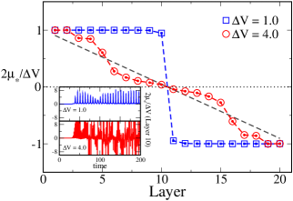
Figure 17: (Color online) Layer-dependent quasiparticle effective chemical potential profile. Parameters are the same of Fig. 15 for $\Delta V=1$ and $\Delta V=4$. The grey dashed line represents the applied bias linear profile. Inset: Real-time dynamics of the quasiparticle chemical potential on the $10^{\text{th}}$ layer. All data are plotted with respect to the leads’ chemical potential absolute value $\Delta V/2$.

IV Conclusions

We used the out-of-equilibrium extension of the inhomogeneous Gutzwiller approximation to study the dynamics of a correlated slab contacted to metal leads in the presence of a voltage bias. On one side this allowed us to investigate the non-equilibrium counterpart of known interface effects arising in strongly correlated heterostructures, such as the dead and living layer phenomena. On the other we studied the non-linear electronic transport of quasiparticles injected into the correlated slab under the influence of an applied bias.

In the first part of the paper we considered a slab in a metallic state in the absence of the bias, when the correlation strength is smaller than the critical value for a Mott transition. Initially we focused on the zero-bias regime and studied the spreading of the doubly occupied sistes injected into the slab after a sudden switch of a tunneling amplitude with the metal leads. Specifically we found a ballistic propagation of the perturbation inside the slab, leaving the system in a stationary state equal to the equilibrium one, with an excess of double occupancies concentrated near the contacts and a consequent enhancement of the quasiparticle weight at the boundaries of the slab. We characterized this “awakening” dynamics of the living layer from the initial dead one in terms of a characteristic time-scale which diverges at the Mott transition. This divergence allow us to identify this timescale as the dynamical counterpart of the equilibrium correlation lenght $\xi$. Borghi et al. (2009)

In the presence of a finite bias we studied the conditions for the formation of non-equilibrium states, characterized by a finite current flowing through the correlated slab. We demonstrated that this process is strongly dependent on the coupling with the external environment represented by the biased metal leads, which at the same time act as the source of the non-equilibrium perturbation and as the only dissipative channel. For weak coupling between the leads and the slab we found stationary currents flowing in a wide range of bias. Conversely for large couplings we identified a strong-bias regime in which the system is trapped into a metastable state characterized by an effective slab-leads decoupling. This is due to an exceedingly fast energy increase and to the lack of strong dissipative processes in the Gutzwiller method, which prevents the injected energy to flow back into the leads and the current to reach a stationary value. Studying the current-bias characteristics in the range of parameter for which the system is able to reach a non equilibrium stationary state, we observed a crossover from a low-bias linear regime, which we find universal with respect to the interaction $U$, to a regime with negative differential conductance typical of finite bandwith systems. Considering suitable long-time averages of the current we have been able to observe the same phenomenology in the region of parameters for which, due to the aforementioned anomalous heating, the current dynamics does not lead to an observable stationary value.

In the second part of this work we turned our attention to the dynamical effect of a bias on a Mott insulating slab, when the interaction strength exceeds the Mott threshold. Following the analysis carried out in the metallic case, we considered the formation of a evanescent bulk quasiparticles after a sudden switch of the slab-leads tunneling amplitude in a zero-bias setup. In this case, we have found that the living layer formation is accompanied by an exponential growth of the quasiparticle weight, suggestive of an avalanche effect determined by the interplay between the dynamics of the quasiparticles and the local degrees of freedom.

In the presence of a finite bias, we studied the conditions under which these evanescent quasiparticles can lead to the opening of a conducting channel through the insulating slab. We showed that at very low bias this is the case only for a very small slab, for which the correlation length $\xi$ is of the same order of the slab size. For larger samples we found that the currents are exponentially activated with a threshold bias $\Delta V_{\mathrm{th}}$ which increases with the slab size. This behavior is suggestive of a Landau-Zener type of dielectric breakdown, as found in previous DMFT studies and in agreement with equilibrium calculations of the tunneling amplitude for a quasiparticle thorugh an insulating slab.

Appendix A Details on the variational dynamics

A straightforward differentiation of Eq. (14) with respect to the variational matrices $\hat{\Phi}_{i}$ leads to the equation of motions

$$\begin{split}&i\frac{\partial}{\partial t}\left(\begin{array}[]{c}\Phi_{z,0}(t)\\ \Phi_{z,1}(t)\\ \Phi_{z,2}(t)\end{array}\right)=\\ &\left(\begin{array}[]{ccc}h_{00}(z,t)&h_{01}(z,t)&0\\ h_{01}^{*}(z,t)&0&h_{01}(z,t)\\ 0&h_{01}^{*}(z,t)&h_{22}(z,t)\end{array}\right)\left(\begin{array}[]{c}\Phi_{z,0}(t)\\ \Phi_{z,1}(t)\\ \Phi_{z,2}(t)\end{array}\right)\end{split}$$ (35)

with

$$\begin{split}h_{00}(z,t)=&\frac{U}{2}-E_{z}+\frac{\delta_{z}}{1-\delta_{z}^{2}}\,\Bigg{\{}2\left|R_{z}\right|^{2}\varepsilon_{z}\\ &-\bigg{[}R^{*}_{z+1}\,R_{z}\,\Delta_{z}\;\big{(}1-\delta_{z,N}\big{)}+c.c.\bigg{]}\\ &-\bigg{[}R^{*}_{z-1}\,R_{z}\,\Delta^{*}_{z-1}\;\big{(}1-\delta_{z,1})+c.c.\bigg{]}\\ &+\bigg{[}\delta_{z,1}\,R^{*}_{1}\,\Gamma_{L}+\delta_{z,N}\,R^{*}_{N}\,\Gamma_{R}+c.c.\bigg{]}\Bigg{\}},\end{split}$$ (36)

$$\begin{split}h_{22}(z,t)=&\frac{U}{2}+E_{z}-\frac{\delta_{z}}{1-\delta_{z}^{2}}\,\Bigg{\{}2\left|R_{z}\right|^{2}\,\varepsilon_{z}\\ &-\bigg{[}R^{*}_{z+1}\,R_{z}\,\Delta_{z}\,\big{(}1-\delta_{z,N})+c.c.\big{)}\bigg{]}\\ &-\bigg{[}R^{*}_{z-1}\,R_{z}\,\Delta^{*}_{z-1}\,\big{(}1-\delta_{z,1}\big{)}+c.c.\bigg{]}\\ &+\bigg{[}\delta_{z,1}R^{*}_{1}\Gamma_{L}+\delta_{z,N}R^{*}_{N}\Gamma_{R}+c.c.\bigg{]}\Bigg{\}},\end{split}$$ (37)

$$\begin{split}h_{01}(z,t)=&\frac{\sqrt{2}}{\sqrt{1-\delta_{z}^{2}}}\bigg{[}R^{*}_{z}\,\varepsilon_{z}-R^{*}_{z+1}\,\Delta_{z}\,\big{(}1-\delta_{z,N}\big{)}\\ &\!\!\!\!\!\!\!\!\!\!\!\!\!\!\!\!\!\!\!\!\!\!-R^{*}_{z-1}\,\Delta^{*}_{z-1}\,\big{(}1-\delta_{z,1}\big{)}+\delta_{z,1}\,\Gamma^{*}_{L}+\delta_{z,N}\,\Gamma^{*}_{R}\bigg{]}.\end{split}$$ (38)

The quantities appearing in the equations of motion (36-38) are defined by quantum averages of fermionic operators over the uncorrelated wavefunction $|{\Psi_{0}(t)}\rangle$

$$\begin{split}&\varepsilon_{z}(t)=\sum_{\mathbf{k}\sigma}\,\langle{\Psi_{0}(t)}|{\,d^{\dagger}_{\mathbf{k}z\sigma}d^{\phantom{\dagger}}_{\mathbf{k}z\sigma}\,}|{\Psi_{0}(t)}\rangle\\ &\Delta_{z}(t)=\sum_{\mathbf{k}\sigma}\,\langle{\Psi_{0}(t)}|{\,d^{\dagger}_{\mathbf{k}z+1\sigma}d^{\phantom{\dagger}}_{\mathbf{k}z\sigma}\,}|{\Psi_{0}(t)}\rangle\\ &\Gamma_{\alpha}(t)=\sum_{\mathbf{k}\sigma}\,\sum_{k_{\perp}}v_{k_{\perp}}\langle{\Psi_{0}(t)}|{\,d^{\dagger}_{\mathbf{k}z_{\alpha}\sigma}c^{\phantom{\dagger}}_{\mathbf{k}k_{\perp}\alpha\sigma}\,}|{\Psi_{0}(t)}\rangle,\end{split}$$ (39)

and their time evolution is determined by the effective Scrödinger equation (10).

To solve for the dynamics of the effective Hamiltonian we introduce the Keldysh Greens’ functions on the uncorrelated wavefunction for $c$ and $d$ operators

$$\mathcal{G}^{K}_{\mathbf{k}\sigma}(z,z^{\prime};t,t^{\prime}) = -i\,\langle{T_{K}\,\bigg{(}d^{\phantom{\dagger}}_{\mathbf{k}z\sigma}(t)\,d^{\dagger}_{\mathbf{k}z^{\prime}\sigma}(t^{\prime})\bigg{)}}\rangle$$ (40)

$$g^{K}_{\mathbf{k}k_{\perp}\alpha\sigma}(z;t,t^{\prime}) = -i\,\langle{T_{K}\,\bigg{(}c^{\phantom{\dagger}}_{\mathbf{k}k_{\perp}\alpha\sigma}(t)d^{\dagger}_{\mathbf{k}z^{\prime}\sigma}(t^{\prime})\bigg{)}}\rangle$$ (41)

and express the quantities in Eqs. 39 in terms of their lesser components computed at equal time

$$\begin{split}\langle{d^{\dagger}_{\mathbf{k}z\sigma}d^{\phantom{\dagger}}_{\mathbf{k}z^{\prime}\sigma}}\rangle(t)=&-i\,\mathcal{G}^{<}_{\mathbf{k}\sigma}(z^{\prime},z;t,t)\\ \langle{d^{\dagger}_{\mathbf{k}z\sigma}c^{\phantom{\dagger}}_{\mathbf{k}k_{\perp}\alpha\sigma}}\rangle(t)=&-i\,g^{<}_{\mathbf{k}k_{\perp}\alpha\sigma}(z;t,t).\end{split}$$ (42)

We compute the equations of motion for the lesser components at equal times, Eq. (42), using the Heisenberg evolution for operators $c$ and $d$ with Hamiltonian $\mathcal{H}_{*}$. In order to get a closed set of differential equations we have to further introduce the dynamics for the leads lesser Green function, which due to the hybridization with the slab lose its translational invariance in the $z$-direction

$$\bigg{[}G^{\alpha\alpha^{\prime}}_{\mathbf{k}k_{\perp}k_{\perp}^{\prime}\sigma}\bigg{]}^{<}(t,t)=i\langle{c^{\dagger}_{\mathbf{k}k_{\perp}\alpha\sigma}c^{\phantom{\dagger}}_{\mathbf{k}k_{\perp}^{\prime}\alpha^{\prime}\sigma}}\rangle.$$ (43)

Dropping, for the sake of simplicity, the lesser symbol and the spin index we get for each $\mathbf{k}$ point the following equations of motion

$$\begin{split}i\partial_{t}\mathcal{G}_{\mathbf{k}}(z,z^{\prime})=&\;\epsilon_{\mathbf{k}}\Big{(}|R_{z}|^{2}-|R_{z^{\prime}}|^{2}\Big{)}\,\mathcal{G}_{\mathbf{k}}(z,z^{\prime})+\sum_{i=\pm 1}\,R_{z+i}^{*}\,R_{z}\,\mathcal{G}_{\mathbf{k}}(z+i,z^{\prime})-R_{z}^{*}\,R_{z+i}\,\mathcal{G}_{\mathbf{k}}(z,z^{\prime}+i)\\ &+\sum_{\alpha=L,R}\,\delta_{z,z_{\alpha}}\,R^{*}_{z_{\alpha}}\,\sum_{k_{\perp}}\,v_{k_{\perp}}^{\alpha}\,g_{\mathbf{k}k_{\perp}}^{\alpha}(z^{\prime})\,+\sum_{\alpha=L,R}\,\delta_{z^{\prime}z_{\alpha}}\,R_{z_{\alpha}}\,\sum_{k_{\perp}}\,v_{k_{\perp}}^{\alpha}\Big{[}g_{\mathbf{k}k_{\perp}}^{\alpha}(z)\Big{]}^{*},\end{split}$$ (44)

$$\begin{split}i\partial_{t}g_{\mathbf{k}k_{\perp}}^{\alpha}(z)=&\;\Big{(}\varepsilon_{\mathbf{k}}^{\alpha}+t_{k_{\perp}}^{\alpha}\Big{)}\,g_{\mathbf{k}k_{\perp}}^{\alpha}(z)-R^{*}_{z+1}\,R_{z}\;g_{\mathbf{k}k_{\perp}}^{\alpha}(z+1)-R^{*}_{z-1}\,R_{z}\;g_{\mathbf{k}k_{\perp}}^{\alpha}(z-1)+v_{k_{\perp}}^{\alpha}\,R_{z_{\alpha}}\,\mathcal{G}_{\mathbf{k}}(z_{\alpha},z)\\ &-\sum_{\alpha^{\prime}=L,R}\,\delta_{z_{\alpha^{\prime}},z}\,\sum_{k_{\perp}}\,v_{k_{\perp}}^{\alpha}\,R_{z_{\alpha^{\prime}}}\,G_{\mathbf{k}k_{\perp}k_{\perp}^{\prime}}^{\alpha\alpha^{\prime}},\end{split}$$ (45)

$$\begin{split}i\partial_{t}G_{\mathbf{k}k_{\perp}k_{\perp}^{\prime}}^{\alpha\alpha^{\prime}}=&\Big{(}t_{k_{\perp}}^{\alpha}-t_{k_{\perp}^{\prime}}^{\alpha^{\prime}}\Big{)}\,G_{\mathbf{k}k_{\perp}k_{\perp}^{\prime}}^{\alpha\alpha^{\prime}}-v_{k_{\perp}^{\prime}}^{\alpha^{\prime}}\,R^{*}_{z_{\alpha^{\prime}}}\;g_{\mathbf{k}k_{\perp}}^{\alpha}(z)-v_{k_{\perp}}^{\alpha}\,R_{z_{\alpha^{\prime}}}\;\Big{[}g_{\mathbf{k}k_{\perp}^{\prime}}^{\alpha^{\prime}}(z)\Big{]}^{*}.\end{split}$$ (46)

The set of differential equations, composed by Eqs. (44-46) and 35, completely determines the dynamics within the time dependendent Gutzwiller and it is solved using a standard 4$-th$ order implicit Runge-Kutta method.H. Brunner and P.J. van der Houven (1986) We mention that this strategy for the solution of the Gutzwiller dynamics correspond to a discretization of the semi-infinite metallic leads. In principle, the latter can be integrated-out exactly at the cost of solving the dynamics for the lesser($<$) and greater($>$) component of the Keldysh Greens’ function on the whole two times $(t,t^{\prime})$-plane. However, such a route can be extremly costly from a computational point of view and restric the simulations to small evolution times. We explicitly checked that the dynamics using the above leads discretization coincides with the dynamics obtained with the two time $(t,t^{\prime})$-plane evolution, up to times for which finite size effects occour. The latter can be however pushed far away with respect to the maximum times reachable within the two time $(t,t^{\prime})$-plane evolution.

Appendix B Landau-Zener stationary tunneling within the Gutzwiller approximation

We believe it is instructive to explicitly show how the Landau-Zener stationary tunnelling across the Mott-Hubbard gap in the presence of a voltage drop translates into the language of the TDG approximation. Here, the gap and the voltage bias are actually absorbed into layer-dependent hopping renormalization factors $R_{z}(t)$ so that, an electron entering the Mott insulating slab from the metal lead translates into a free quasiparticle with hopping parameters that decay exponentially inside the insulator. In other words, quasiparticles within the Gutzwiller approximation do not experience a tunneling barrier in the insulating side but rather an exponentially growing mass.

From this viewpoint, the living layer that appears at the metal-Mott insulator interface can be legitimately regarded as the evanescent wave yielded by tunnelling across the Mott-Hubbard gap. Such a correspondence can be made more explicit following Ref. Borghi et al., 2010 and its Supplemental Material.

Specifically, we shall consider a single metal-Mott insulator interface at equilibrium, with the metal and the Mott insulator confined in the regions $z<0$ and $z\geq 0$, respectively. The new ingredient that we add with respect to Ref. Borghi et al., 2010 is an electrochemical potential $\mu(z)$, which is constant and for convenience zero on the metal side, i.e. $\mu(z<0)=0$, while finite on the insulating side, $\mu(z\geq 0)\not=0$, thus mimicking the bending of the Mott-Hubbard side bands at the junction.

If the correlation length $\xi$ of the Mott insulator is much bigger that the inverse Fermi wavelength, in the Gutzwiller approach we can further neglect as a first approximation the $z$-dependence of the averages of hopping operators over the uncorrelated Slater determinant $\mid\!\Psi_{0}\rangle$. Borghi et al. (2010) We can thus write the energy of the system as a functional of the variational matrices only,

$$E = -\frac{2}{24\,L}\,\sum_{z}\,R(z)^{2}-\frac{1}{24\,L}\sum_{z}\,R(z)\,R(z+1)+\frac{\displaystyle 1}{\displaystyle 2\,L}\,\sum_{z}\,U(z)\,\Big{(}\mid\!\Phi_{0}(z)\!\mid^{2}+\mid\!\Phi_{2}(z)\!\mid^{2}\Big{)}-\frac{1}{L}\,\sum_{z}\,\mu(z)\,\delta(z),\;\;$$ (47)

where

$$R(z) = \sqrt{\frac{\displaystyle 2}{\displaystyle 1-\delta(z)^{2}}}\;\;\Big{(}\Phi_{1}(z)^{*}\,\Phi_{0}(z)^{\phantom{\dagger}}+\Phi_{2}(z)^{*}\,\Phi_{1}(z)^{\phantom{\dagger}}\Big{)},$$

is the hopping renormalization factor, and

$$\delta(z)=\mid\Phi_{0}(z)\mid^{2}-\mid\Phi_{2}(z)\mid^{2},$$

is the doping of layer $z$ with respect to half-filling, i.e. $n(z)=1-\delta(z)$. We have chosen units such that the Mott transition occurs at $U=1$, so that $U(z<0)=U_{\text{metal}}\ll 1$ on the metal side, and $U(z\geq 0)=U\gtrsim 1$ on the insulating one.

The minimum of $E$ in Eq. (47) can be always found with real parameters $\Phi_{n}(z)$, so that, since

$$\Phi_{0}(z)^{2}+\Phi_{1}(z)^{2}+\Phi_{2}(z)^{2}=1,$$

there are actually two independent variables per layer. We can always choose these variables as $R(z)\in[0,1]$ and $\delta(z)\in[-1,1]$, in which case

$$\mid\Phi_{0}(z)\mid^{2}+\mid\Phi_{2}(z)\mid^{2} = \frac{\displaystyle 1}{\displaystyle 2}\,\Bigg{(}\Xi\big{[}R(z),\delta(z)\big{]}$$

$$\qquad\qquad+\frac{\displaystyle\delta(z)^{2}}{\displaystyle\Xi\big{[}R(z),\delta(z)\big{]}}\Bigg{)},$$

where

$$\Xi\big{[}R(z),\delta(z)\big{]} = 1-\sqrt{1-R(z)^{2}}\;\;\sqrt{1-\delta(z)^{2}}$$

$$\simeq 1-\sqrt{1-R(z)^{2}}+\frac{\displaystyle\delta(z)^{2}}{\displaystyle 2}\,\sqrt{1-R(z)^{2}},$$

the last expression being valid for small doping. Minimizing $E$ in Eq. (47) with respect to $\delta(z)$ leads to

$$\delta(z) \simeq \frac{\displaystyle 4\mu(z)}{\displaystyle U}\;\frac{\displaystyle 1-\sqrt{1-R(z)^{2}}}{\displaystyle 1+R(z)^{2}+\sqrt{1-R(z)^{2}}},$$ (48)

for $z\geq 0$, and $\delta(z)=0$ for $z<0$.

Through Eq. (48) we find an equation for $R(z)$ in the insulating side $z\geq 0$ that, after taking the continuum limit, reads

$$\frac{\displaystyle\partial^{2}R(z)}{\displaystyle\partial z^{2}}=-\frac{\displaystyle\partial}{\displaystyle\partial R(z)}\;V\Big{[}R(z),z\Big{]},$$ (49)

which looks like a classical equation of motion with $z$ playing the role of time $t$, $R(z)$ that of the coordinate $q(t)$, and $V$ that of a time-dependent potential

$$V\big{(}q,t\big{)} = -6U\,\bigg{(}1-\sqrt{1-q^{2}}\bigg{)}+3q^{2}$$ (50)

$$+\frac{\displaystyle 48\mu(t)^{2}}{\displaystyle U}\;\frac{\displaystyle 1-\sqrt{1-q^{2}}}{\displaystyle 1+q^{2}+\sqrt{1-q^{2}}}.$$

On the metallic side $R(z<0)\simeq R_{\text{metal}}\simeq 1$, so that the role of the junction is translated into appropriate boundary conditions at $z=0$.

Far inside the insulator, $R(z)\ll 1$ and we can expand

$$V\Big{[}R(z),z\Big{]} \simeq \left(-3U+3+24\,\frac{\displaystyle\mu(z)^{2}}{\displaystyle U}\right)\,R(z)^{2},$$

so that the linearized equation reads

$$\frac{\displaystyle\partial^{2}R(z)}{\displaystyle\partial z^{2}}=\left[6U-6-\frac{\displaystyle 48}{\displaystyle U}\;\mu(z)^{2}\right]\;R(z),$$ (51)

for $z>0$, while, in the metal side, $z<0$, where $R(z)$ is approximately constant,

$$\frac{\displaystyle\partial^{2}R(z)}{\displaystyle\partial z^{2}}=0.$$ (52)

Equations (51) and (52) can be regarded as the Shrœdinger equation of a zero-energy particle impinging on a potential barrier at $z\geq 0$. Within the WKB approximation, the transmitted wavefunction at $z$ reads

$$R(z)\propto\exp\bigg{(}-\int_{0}^{z_{*}}\,d\zeta\,\sqrt{6U-6-\frac{\displaystyle 48}{\displaystyle U}\;\mu(\zeta)^{2}}\;\bigg{)},\;\;\;$$ (53)

where, assuming a monotonous $\mu(\zeta)$, the upper limit of integration is $z_{*}=z$ if $8\mu(z)^{2}\leq U\,(U-1)$ otherwise is the turning point, i.e. $z_{*}$ such that $8\mu(z_{*})^{2}=U\,(U-1)$.

Let us for instance take $\mu(z)=\text{E}\,z$, which corresponds to a constant electric field. In this case

$$|\text{E}|\,z_{*}=\sqrt{\frac{\displaystyle U(U-1)}{\displaystyle 8}},$$ (54)

so that the transmission probability

$$\left|R(z>z_{*})\right|^{2}\sim\exp\Bigg{(}-\frac{\displaystyle E_{\text{th}}}{\displaystyle E}\Bigg{)},$$ (55)

where the threshold field

$$E_{\text{th}}=\frac{\displaystyle\pi}{\displaystyle 2}\;\sqrt{\frac{\displaystyle U}{\displaystyle 48}}\;\xi^{-2},$$ (56)

with the definition of the correlation length $\xi^{-1}=\sqrt{6(U-1)}$ of Ref. Borghi et al., 2010.

We observe that Eq. (55) has exactly the form predicted by the Zener tunnelling in a semiconductor upon identifying

$$E_{g}\,\sqrt{\frac{\displaystyle m_{*}\,E_{g}}{\displaystyle\hbar^{2}}}\sim U-U_{c},$$ (57)

where $E_{g}$ is the semiconductor gap, $m_{*}$ the mass parameter and $U_{c}$ the dimensional value of the interaction at the Mott transition.

B.1 Growth of the living layer

The same approximate approach just outlined can be also extended away from equilibrium. We shall here consider the simple case of constant and vanishing electrochemical potential $\mu(z)=0$. We need to find the saddle point of the action

$$S=\int dt\,i\sum_{n=0}^{2}\sum_{z}\,\Phi_{n}(z,t)^{*}\,\dot{\Phi}_{n}(z,t)^{\phantom{\dagger}}-E(t),$$ (58)

where $E(t)$ is the same functional of Eq. (47) where now all parameters $\Phi_{n}(z,t)$ are also time dependent. At $\mu(z)=0$ we can set

$$\Phi_{0}(z,t) = \Phi_{2}(z,t)=\frac{\displaystyle 1}{\displaystyle\sqrt{2}}\;\text{e}^{i\phi(z,t)}\;\sin\frac{\displaystyle\theta(z,t)}{\displaystyle 2},$$ (59)

$$\Phi_{1}(t) = \cos\frac{\displaystyle\theta(z,t)}{\displaystyle 2},$$ (60)

so that the equations of motion read

$$\sin\theta(z,t)\,\dot{\phi}(z,t) = -2\,\frac{\displaystyle\partial E}{\displaystyle\partial\theta(z,t)},$$ (61)

$$\sin\theta(z,t)\,\dot{\theta}(z,t) = 2\,\frac{\displaystyle\partial E}{\displaystyle\partial\phi(z,t)}.$$ (62)

Upon introducing the parameters

$$\sigma_{x}(z,t) = \sin\theta(z,t)\,\cos\phi(z,t),$$ (63)

$$\sigma_{y}(z,t) = \sin\theta(z,t)\,\sin\phi(z,t),$$ (64)

$$\sigma_{z}(z,t) = \cos\theta(z,t),$$ (65)

where $\sigma_{x}(z,t)=R(z,t)$ is the time dependent hopping renormalizaton, the equations of motion can be written as

$$\dot{\sigma}_{x}(z,t) = -2\sigma_{y}(z,t)\,\frac{\displaystyle\partial E}{\displaystyle\partial\sigma_{z}(z,t)}=\frac{U}{2}\,\sigma_{y}(z,t),$$ (66)

$$\dot{\sigma}_{y}(z,t) = 2\sigma_{x}(z,t)\,\frac{\displaystyle\partial E}{\displaystyle\partial\sigma_{z}(z,t)}-2\sigma_{z}(z,t)\,\frac{\displaystyle\partial E}{\displaystyle\partial\sigma_{x}(z,t)}$$ (67)

$$=-\frac{U}{2}\,\sigma_{x}(z,t)-2\sigma_{z}(z,t)\,\frac{\displaystyle\partial E}{\displaystyle\partial\sigma_{x}(z,t)},$$

$$\dot{\sigma}_{z}(z,t) = 2\sigma_{y}(z,t)\,\frac{\displaystyle\partial E}{\displaystyle\partial\sigma_{x}(z,t)},$$ (68)

where

$$\frac{\displaystyle\partial E}{\displaystyle\partial\sigma_{x}(z,t)} = -\frac{1}{6}\,\sigma_{x}(z,t)-\frac{1}{24}\,\Big{(}\sigma_{x}(z+1,t)+\sigma_{x}(z-1,t)\Big{)}$$ (69)

$$\simeq-\frac{1}{4}\,\sigma_{x}(z,t)-\frac{1}{24}\,\frac{\displaystyle\partial^{2}\sigma_{x}(z,t)}{\displaystyle\partial z^{2}}.$$

The Eqs. (66)–(68) show that the Gutzwiller equations of motion actually coincide to those of a Ising model in a transverse field treated within mean-field, as originally observed in Ref. Schiró and Fabrizio, 2010.

Inside the Mott insulating slab we can safely assume $\sigma_{z}(z,t)\sim 1$ and obtain the equation for $R(z,t)=\sigma_{x}(z,t)$

$$\ddot{R}(z,t)=-\frac{U}{4}\,\big{(}U-1\big{)}\,R(z,t)+\frac{\displaystyle U}{\displaystyle 24}\,\frac{\displaystyle\partial^{2}R(z,t)}{\displaystyle\partial z^{2}},$$ (70)

which is the time dependent version of Eq. (51) and is just a Klein-Gordon equation

$$\frac{\displaystyle 1}{\displaystyle c^{2}}\,\ddot{R}-\nabla^{2}\,R+m^{2}\,c^{2}\,R=0,$$ (71)

with light velocity $c$ and mass $m$ given by

$$c^{2} = U/24,$$ (72)

$$m^{2}\,c^{2} = 6\,\big{(}U-1\big{)}=\xi^{-2}.$$ (73)

In dimensionless units

$$\frac{\displaystyle z}{\displaystyle\xi}\rightarrow z,\qquad\frac{\displaystyle ct}{\displaystyle\xi}\rightarrow t.$$

Eq. (71) reads

$$\ddot{R}-\nabla^{2}\,R+R=0.$$ (74)

Let us simulate the growth of the ”living layer” by a single metal-Mott insulator interface and absorb the role of the metal into an appropriate boundary condition for the surface $z=0$ of the Mott insulator side $z\geq 0$. Specifically, we shall assume that initially $R(z,0)=R_{0}(z)$, with $R_{0}(0)=R_{0}>0$ and $R_{0}(z\to\infty)=0$, as well as that, at any time $t$, the value of $R(z,t)$ at the surface remains constant, i.e. $R(0,t)=R_{0}$, $\forall t$. We denote as $R_{*}(z)$ the stationary solution of Eq. (74) with the boundary condition $R_{*}(0)=R_{0}$, that is

$$R_{*}(z)=R_{0}\,\text{e}^{-z}.$$ (75)

One can readily obtain a solution of Eq. (74) satisfying all boundary condition, which, after defining

$$\phi(x)=R_{0}(x)-R_{*}(x),$$ (76)

reads

$$R(z,t) = R_{*}(z)+\frac{\displaystyle\phi(z+t)+\theta(z-t)\,\phi(z-t)-\theta(t-z)\,\phi(t-z)}{\displaystyle 2}$$

$$-\frac{t}{2}\,\int_{-t}^{t}\,dx\;\frac{\displaystyle J_{1}\Big{(}\sqrt{t^{2}-x^{2}}\,\Big{)}}{\displaystyle\sqrt{t^{2}-x^{2}}}\Big{[}\theta(x+z)\,\phi(x+z)-\theta(x-z)\,\phi(x-z)\Big{]},$$

where $J_{1}(x)$ is the first order Bessel function. We observe that for very long times $R(z,t\to\infty)\to R_{*}(z)$, namely the solution evolves into a steady state that corresponds to the equilibrium evanescent wave with the appropriate boundary condition. Moreover, Eq.  (B.1) also shows a kind of light-cone effect compatible with the full evolution that takes into account also the dynamics of the Slater determinant, which we have neglected to get Eq. (74). In fact, the missing Slater determinant dynamics is the reason why the initial exponential growth is not captured by Eq. B.1, which thence has to be rather regarded as an asymptotic description valid only at long time and distances.

Another possible boundary condition is to impose that $\partial_{z}R(z,t)$ remains constant at $z=0$, rather than its value. In this case, if

$$A=-\frac{\displaystyle\partial R(z,0)}{\displaystyle\partial z}_{z=0}=-\frac{\displaystyle\partial R_{0}(z)}{\displaystyle\partial z}_{z=0}\;,$$ (78)

then we must take $R_{*}(z)=A\,\text{e}^{-z}$ and still $\phi(x)=R_{0}(x)-R_{*}(x)$ so that the solution reads

$$R(z,t) = R_{*}(z)+\frac{\displaystyle\phi(z+t)+\theta(z-t)\,\phi(z-t)+\theta(t-z)\,\phi(t-z)}{\displaystyle 2}$$

$$-\frac{t}{2}\,\int_{-t}^{t}\,dx\;\frac{\displaystyle J_{1}\Big{(}\sqrt{t^{2}-x^{2}}\,\Big{)}}{\displaystyle\sqrt{t^{2}-x^{2}}}\Big{[}\theta(x+z)\,\phi(x+z)+\theta(x-z)\,\phi(x-z)\Big{]}.$$

Also in this case $R(z,t)$ evolves towards a stationary value that, in dimensional units, reads

$$R(z,t\to\infty)=A\,\xi\,\text{e}^{-z/\xi},$$ (80)

hence growths exponentially at fixed $A$ and $z$ as the Mott transition is approached.

References

- Bednorz and Müller (1986) J. G. Bednorz and K. A. Müller, Zeit. Phys. B 64, 189 (1986).
- Anderson (1997) P. W. Anderson, The Theory of Superconductivity in High-Tc Cuprates (Princeton University Press., 1997).
- Kamihara et al. (2008) Y. Kamihara, T. Watanabe, M. Hirano, and H. Hosono, J. Am. Chem. Soc. 130, 3296 (2008).
- Mott (1968) N. F. Mott, Rev. Mod. Phys. 40, 677 (1968).
- Imada et al. (1998) M. Imada, A. Fujimori, and Y. Tokura, Rev. Mod. Phys. 70, 1039 (1998).
- Okamoto and Millis (2004) S. Okamoto and A. Millis, Phys. Rev. B 70, 241104 (2004).
- Ishida and Liebsch (2008) H. Ishida and A. Liebsch, Phys. Rev. B 77, 115350 (2008).
- Biscaras et al. (2010) J. Biscaras, N. Bergeal, A. Kushwaha, T. Wolf, A. Rastogi, R. C. Budhani, and J. Lesueur, Nat. Commun. 1, 89 (2010).
- Zubko et al. (2011) P. Zubko, S. Gariglio, M. Gabay, P. Ghosez, and J.-M. Triscone, Annual Review of Condensed Matter Physics 2, 141 (2011).
- Tsymbal et al. (2012) E. Y. Tsymbal, E. Dagotto, E. Chang-Beom, and R. Ramamoorthy, eds., Multifunctional Oxide Heterostructures (Oxford University Press, 2012).
- Sulpizio et al. (2014) J. A. Sulpizio, S. Ilani, P. Irvin, and J. Levy, Annual Review of Materials Research 44, 117 (2014).
- Freericks (2004) J. Freericks, Phys. Rev. B 70, 1 (2004).
- Rodolakis et al. (2009) F. Rodolakis, B. Mansart, E. Papalazarou, S. Gorovikov, P. Vilmercati, L. Petaccia, A. Goldoni, J. P. Rueff, S. Lupi, P. Metcalf, et al., Phys. Rev. Lett. 102, 066805 (2009).
- Borghi et al. (2009) G. Borghi, M. Fabrizio, and E. Tosatti, Phys. Rev. Lett. 102, 066806 (2009).
- Orenstein (2012) J. Orenstein, Phys. Today 65, 44 (2012).
- Guiot et al. (2013) V. Guiot, L. Cario, E. Janod, B. Corraze, V. Ta Phuoc, M. Rozenberg, P. Stoliar, T. Cren, and D. Roditchev, Nat. Commun. 4, 1722 (2013).
- Aoki et al. (2014) H. Aoki, N. Tsuji, M. Eckstein, M. Kollar, T. Oka, and P. Werner, Rev. Mod. Phys. 86, 779 (2014).
- Okamoto (2007) S. Okamoto, Phys. Rev. B 76, 035105 (2007).
- Okamoto (2008) S. Okamoto, Phys. Rev. Lett. 101, 116807 (2008).
- Heary and Han (2009) R. J. Heary and J. Han, Phys. Rev. B 80, 035102 (2009).
- Li et al. (2014) J. Li, C. Aron, G. Kotliar, and J. E. Han, ArXiv e-prints (2014), eprint 1410.0626.
- Amaricci and Capone (2014) A. Amaricci and M. Capone, ArXiv e-prints (2014), eprint 1411.2347.
- Joura et al. (2008) A. V. Joura, J. K. Freericks, and T. Pruschke, Phys. Rev. Lett. 101, 196401 (2008).
- Amaricci et al. (2012) A. Amaricci, C. Weber, M. Capone, and G. Kotliar, Phys. Rev. B 86, 085110 (2012).
- Tsuji et al. (2008) N. Tsuji, T. Oka, and H. Aoki, Phys. Rev. B 78, 235124 (2008).
- Tsuji et al. (2011) N. Tsuji, T. Oka, P. Werner, and H. Aoki, Phys. Rev. Lett. 106, 5 (2011), eprint 1008.2594.
- Eckstein et al. (2010) M. Eckstein, T. Oka, and P. Werner, Phys. Rev. Lett. 105, 146404 (2010).
- Schiró and Fabrizio (2010) M. Schiró and M. Fabrizio, Phys. Rev. Lett 105, 076401 (2010).
- André et al. (2012) P. André, M. Schiró, and M. Fabrizio, Phys. Rev. B 85, 205118 (2012).
- Eckstein and Werner (2013) M. Eckstein and P. Werner, Phys. Rev. B 88, 075135 (2013).
- Eckstein and Werner (2014) M. Eckstein and P. Werner, Phys. Rev. Lett. 113, 076405 (2014).
- Oka and Aoki (2005) T. Oka and H. Aoki, Phys. Rev. Lett. 95, 137601 (2005).
- Oka et al. (2003) T. Oka, R. Arita, and H. Aoki, Phys. Rev. Lett. 91, 066406 (2003).
- Charlebois et al. (2013) M. Charlebois, S. R. Hassan, R. Karan, D. Sénéchal, and A.-M. S. Tremblay, Phys. Rev. B 87, 035137 (2013).
- Chen and Freericks (2007) L. Chen and J. K. Freericks, Phys. Rev. B 75, 125114 (2007).
- Fabrizio (2013) M. Fabrizio, in New Materials for Thermoelectric Applications: Theory and Experiment, edited by V. Zlatic and A. Hewson (Springer Netherlands, 2013), NATO Science for Peace and Security Series B: Physics and Biophysics, pp. 247–273.
- Borghi et al. (2010) G. Borghi, M. Fabrizio, and E. Tosatti, Phys. Rev. B 81, 115134 (2010).
- Eckstein et al. (2009) M. Eckstein, M. Kollar, and P. Werner, Phys. Rev. Lett. 103, 056403 (2009).
- Sandri et al. (2012) M. Sandri, M. Schiró, and M. Fabrizio, Phys. Rev. B 86, 075122 (2012).
- Mazza and Fabrizio (2012) G. Mazza and M. Fabrizio, Phys. Rev. B 86, 184303 (2012).
- Aron et al. (2012) C. Aron, G. Kotliar, and C. Weber, Phys. Rev. Lett. 108, 086401 (2012).
- Mierzejewski et al. (2011) M. Mierzejewski, L. Vidmar, J. Bonča, and P. Prelovšek, Phys. Rev. Lett. 106, 196401 (2011).
- Arrigoni et al. (2013) E. Arrigoni, M. Knap, and W. von der Linden, Phys. Rev. Lett. 110, 086403 (2013).
- Lanatà (2010) N. Lanatà, Phys. Rev. B 82, 195326 (2010).
- Zenia et al. (2009) H. Zenia, J. K. Freericks, H. R. Krishnamurthy, and T. Pruschke, Phys. Rev. Lett. 103, 116402 (2009).
- H. Brunner and P.J. van der Houven (1986) H. Brunner and P.J. van der Houven, The numerical solution of Volterra Equations (North-Holland, Amsterdam, 1986).