Enhancing SfePy with Isogeometric Analysis

Abstract

In the paper a recent enhancement to the open source package SfePy (Simple Finite Elements in Python, http://sfepy.org) is introduced, namely the addition of another numerical discretization scheme, the isogeometric analysis, to the original implementation based on the nowadays standard and well-established numerical solution technique, the finite element method. The isogeometric removes the need of the solution domain approximation by a piece-wise polygonal domain covered by the finite element mesh, and allows approximation of unknown fields with a higher smoothness then the finite element method, which can be advantageous in many applications. Basic numerical examples illustrating the implementation and use of the isogeometric analysis in SfePy are shown.

1 Introduction

Many problems in physics, biology, chemistry, geology and other scientific disciplines can be described mathematically using a partial differential equation (PDE) or a system of several PDEs. The PDEs are formulated in terms of unknown field variables or fields, defined in some domain with a sufficiently smooth boundary embedded in physical space.

SfePy (Simple Finite Elements in Python, http://sfepy.org) is a framework for solving various kinds of problems (mechanics, physics, biology, …) described by PDEs in two or three space dimensions. Because only the most basic PDEs on simple domains (circle, square, etc.) can be solved analytically, a numerical solution scheme is needed, involving, typically:

• an approximation of the original domain by a polygonal domain;

• an approximation of continuous fields by discrete fields defined by a finite set of degrees of freedom (DOFs) and a (piece-wise) polynomial basis.

The above steps are called discretization of the continuous problem. In the following text two discretization schemes will be briefly outlined:

• the finite element method [FEM] - a long-established industry approved method based on piece-wise polynomial approximation,

• the isogeometric analysis [IGA] - a quite recent generalization of FEM that uses spline- or NURBS-based approximation.

SfePy, as its name suggests, has been based on FEM from its very beginning. The IGA implementation has been added mainly due to the following reasons (both will be addressed more in the text):

• The IGA approximation can be globally smooth on a single patch geometry. The continuity is determined by a few well defined parameters. This fact was the main factor in deciding to implement IGA, because the smoothness is crucial in one of our research applications (ab-initio electronic structure calculations - work in progress). The high smoothness is paid for by the higher computational complexity of the NURBS basis evaluation and higher fill-in of the sparse matrix that a problem discretization leads to.

• IGA can work directly with the geometric description of objects used in geometric modeling and computer-aided design (CAD) systems, removing thus the meshing step.

The paper is structured as follows. The geometric representation of objects is outlined in Geometry Description using NURBS, because the terms defined there are used in the IGA part of Outline of FEM and IGA. Then the particular choices made in SfePy are presented in IGA Implementation in SfePy and illustrated using examples of PDE solutions in Examples. All computations below were done in SfePy, version 2014.3 - note that this paper is a short description of the state and capabilities of the code as of this version. The examples of numerical solutions have no particular scientific meaning or importance besides being an illustration of the used methods.

2 Geometry Description using NURBS

First, let us briefly review the geometric representation of objects using Bézier curves, B-splines and [NURBS] (Non-uniform rational B-spline) curves and 2D (surface) or 3D (solid) bodies, to elucidate terminology used in subsequent sections. Our IGA implementation is based on the explanation and algorithms in [BE], thus below we follow its notation and definitions.

2.1 Bézier Curves

A Bézier curve is a parametric curve frequently used in computer graphics and related fields. We define it here because its polynomial basis is used in the code by means of the Bézier extraction technique, see [BE] and below.

A degree $p$ Bézier curve is defined by a linear combination of $p+1$ Bernstein polynomial basis functions as

$$C(\xi)=\sum_{a=1}^{p+1}\bm{P}_{a}B_{a,p}(\xi)=\bm{P}^{T}\bm{B}(\xi)\mbox{ for }\xi\in[0,1]\;,$$

where $\bm{P}=\{\bm{P}_{a}\}_{a=1}^{p+1}$ is the set of control points and $\bm{B}(\xi)=\{B_{a,p}(\xi)\}_{a=1}^{p+1}$ is the set of Bernstein polynomial basis functions. The Bernstein basis can be defined recursively for $\xi\in[0,1]$ as $B_{a,p}(\xi)=(1-\xi)B_{a,p-1}(\xi)+\xi B_{a-1,p-1}(\xi)$, $B_{1,0}(\xi)\equiv 1$, $B_{a,p}(\xi)\equiv 0$ if $a<1$ or $a>p+1$. An example of Bézier curve is shown in Fig. 1.

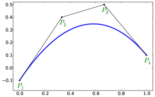
Figure 1: A Bézier curve (blue) of degree three with four control points in two space dimensions.

2.2 B-spline Curves

A B-spline is a generalization of the Bézier curve. B-splines (and their NURBS generalization, see below) are used in computer graphics, geometry modeling and related fields as well as the Bézier curves. In IGA B-spline basis functions can be used for approximation of the unknown fields.

A univariate B-spline curve of degree $p$ is defined by a linear combination of $n$ basis functions as

$$T(\xi)=\sum_{A=1}^{n}\bm{P}_{A}N_{A,p}(\xi)=\bm{P}^{T}\bm{N}(\xi)\;,$$

where $\bm{P}=\{\bm{P}_{A}\}_{A=1}^{n}$ is the set of control points. The basis functions are defined by a knot vector - a set of non-decreasing parametric coordinates $\Xi=\{\xi_{1},\xi_{2},\dots,\xi_{n+p+1}\}$, where $\xi_{A}\in\mathbb{R}$ is the $A^{th}$ knot and $p$ is the polynomial degree of the B-spline basis functions. Then for $p=0$

$$N_{A,0}(\xi) = 1\mbox{ for }\xi_{A}\leq\xi<\xi_{A+1}\;,$$

$$= 0\mbox{ otherwise.}$$

For $p>0$ the basis functions are defined by the Cox-de Boor recursion formula

$$N_{A,p}(\xi)=\frac{\xi-\xi_{A}}{\xi_{A+p}-\xi_{A}}N_{A,p-1}(\xi)+\frac{\xi_{A+p+1}-\xi}{\xi_{A+p+1}-\xi_{A+1}}N_{A+1,p-1}(\xi)\;.$$

Note that it is possible to insert knots into a knot vector without changing the geometric or parametric properties of the curve by computing the new set of control points in a particular way, see e.g. [BE].

A B-spline curve with a knot vector with no internal knots, i.e. of the form

$$\Xi=\{\underbrace{0,\dots,0}_{p+1},\underbrace{1,\dots,1}_{p+1}\}\;,$$

corresponds to a Bézier curve of degree $p$ with the same control points.

2.3 NURBS Curves

B-splines can be used to approximately describe almost any geometry. Their main drawback is the fact, that a circular or spherical segment cannot be described exactly. This problem was eliminated by the introduction of NURBS in geometry modelling.

A NURBS (Non-uniform rational B-spline) of degree $p$ is defined by a linear combination of $n$ rational basis functions as

$$T(\xi)=\sum_{A=1}^{n}\bm{P}_{A}R_{A,p}(\xi)=\bm{P}^{T}\bm{R}(\xi)\;,$$

where $\bm{P}=\{\bm{P}_{A}\}_{A=1}^{n}$ is the set of control points and $\bm{R}(\xi)=\{R_{A,p}(\xi)\}_{A=1}^{p+1}$ is the set of rational basis functions. The rational basis functions are defined using the B-spline basis functions as

$$R_{A,p}(\xi)=\frac{w_{A}{N_{A,p}(\xi)}}{W(\xi)}\;,\quad W(\xi)=\sum_{B=1}^{n}w_{B}N_{B,p}(\xi)\;,$$

where $w_{i}$ is the weight corresponding to the $i^{th}$ basis function and $W$ is the weight function.

Note that a NURBS curve in $\mathbb{R}^{n}$ is equal to a B-spline curve in $\mathbb{R}^{n+1}$:

$$T(\xi)=\sum_{A=1}^{n}\bar{\bm{P}_{A}}N_{A,p}(\xi)\;,\quad\bar{\bm{P}_{A}}=\{w_{A}\bm{P}_{A},w_{A}\}^{T}\;.$$

This means that all algorithms that work for B-splines work also for NURBS.

2.3.1 NURBS Surfaces and Solids

A surface is obtained by the tensor product of two NURBS curves. The knot vector is defined for each axial direction and there are $n\times m$ control points for $n$ basis functions in the first axis and $m$ basis functions in the second one.

Analogically, a solid is given by tensor product of three NURBS curves.

2.3.2 NURBS Patches

Complex geometries cannot be described by a single NURBS outlined above, often called NURBS patch - many such patches might be needed, and special care must be taken to ensure required continuity along patch boundaries and to avoid holes. A single patch geometry will be used in the following text, see Fig. 2.

3 Outline of FEM and IGA

The two discretization methods will be illustrated on a very simple PDE - the Laplace equation - in a plane (2D) domain. The Laplace equation describes diffusion and can be used to determine, for example, temperature or electrical potential distribution in the domain. We will use the "temperature" terminology and the notation from Table I.

symbol	meaning
$\Omega$	solution domain
$\Omega_{h}$	discretized solution domain
$\Gamma_{D}$, $\Gamma_{N}$	subdomains representing parts of the domain surface for applying Dirichlet and Neumann boundary conditions
$\underline{n}$	unit outward normal
$\nabla\equiv[\frac{\partial}{\partial x_{1}},\frac{\partial}{\partial x_{2}}]^{T}$	gradient operator
$\nabla\cdot$	divergence operator
$\Delta\equiv\nabla\cdot\nabla$	Laplace operator
$C^{1}$	space of functions with continuous first derivatives
$H^{1}$	space of functions with integrable values and first derivatives
$H^{1}_{0}$	space of functions from $H^{1}$ that are zero on $\Gamma_{D}$

TABLE II: Notation.

The problem is as follows: Find temperature $T$ such that:

$$\Delta T = 0\mbox{ in }\Omega\;,$$ (1)

$$T = \bar{T}\mbox{ on }\Gamma_{D}\;,$$ (2)

$$\nabla T\cdot\underline{n} = 0\mbox{ on }\Gamma_{N}\;,$$ (3)

where the second equation is the Dirichlet (or essential) boundary condition and the third equation is the Neumann (or natural) boundary condition that corresponds to a flux through the boundary.

The operator $\Delta$ has second derivatives - that means that the solution $T$ needs to have continuous first derivatives, or, it has to be from $C^{1}$ function space - this is often not possible in examples from practice. Instead, a weak solution is sought that satisfies: Find $T\in H^{1}(\Omega)$

$$\int_{\Omega}\nabla s\cdot\nabla T-\underbrace{\int_{\Gamma_{N}}s\ \nabla T\cdot\underline{n}}_{\equiv 0} = 0\;,\quad\forall s\in H^{1}_{0}(\Omega)\;,$$ (4)

$$T = \bar{T}\quad\mbox{ on }\Gamma_{D}\;,$$ (5)

where the natural boundary condition appears naturally in the equation (hence its name). The above system can be derived by multiplying the original equation by a test function $s\in H^{1}_{0}(\Omega)$, integrating over the whole domain and then integrating by parts.

Both FEM and IGA now replace the infinite function space $H^{1}(\Omega)$ by a finite subspace with a basis with a small support on a discretized domain $\Omega_{h}$, see below for particular basis choices. Then $T(\underline{x})\approx\sum_{k=1}^{N}T_{k}\phi_{k}(\underline{x})$, where $T_{k}$ are the DOFs and $\phi_{k}$ are the base functions. Similarly, $s(\underline{x})\approx\sum_{k=1}^{N}s_{k}\phi_{k}(\underline{x})$. Substituting those into (4) we obtain

$$\int_{\Omega_{h}}\left(\sum_{j=1}^{N}s_{j}\nabla\phi_{j}\cdot\sum_{k=1}^{N}\nabla\phi_{k}T_{k}\right)=0\;.$$

This has to hold for any $s$, so we can choose $s=\phi_{j}$ for $j=1,\dots,N$. It is also possible to switch the sum with the integral and put the constants $T_{k}$ out of the integral, to obtain the discrete system:

$$\sum_{k=1}^{N}\int_{\Omega_{h}}\left(\nabla\phi_{j}\cdot\nabla\phi_{k}\right)T_{k}=0\;.$$ (6)

In compact matrix notation we can write $\bm{K}\bm{T}=\bm{0}$, where the matrix $\bm{K}$ has components $K_{ij}=\int_{\Omega_{h}}\nabla\phi_{i}\cdot\nabla\phi_{j}$ and $\bm{T}$ is the vector of $T_{k}$. The Dirichlet boundary conditions are satisfied by setting the $T_{k}$ on the boundary $\Gamma_{D}$ to appropriate values.

Both methods make use of the small support and evaluate (6) as a sum over small "elements" to obtain local matrices or vectors that are then assembled into a global system - system of linear algebraic equations in our case.

The particulars of domain geometry description and basis choice will now be outlined. For both methods, we will use the domain shown in Figure 2. Its geometry is described by NURBS, see Geometry Description using NURBS.

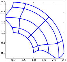
Figure 2: The domain with a curved boundary described by NURBS. The internal lines correspond to several selected iso-lines given by the parametrization of the 2D tensor-product NURBS patch.

3.1 FEM

In this method a continuous solution domain is approximated by a polygonal domain - FE mesh - composed of small basic subdomains with a simple geometric shape (e.g. triangles or quadrilaterals in 2D, tetrahedrons or hexahedrons in 3D) - the elements. The continuous fields of the PDEs are approximated by polynomials defined on the individual elements. This approximation is (usually) continuous over the whole domain, but its derivatives are only piece-wise continuous.

First we need to make a FE mesh from the NURBS description, usual in CAD systems. While it is easy for our domain, it is a difficult task in general, especially in 3D space. Here a cheat has been used and the mesh depicted in Figure 3 was generated from the NURBS description using the IGA techniques described below. Quite a fine mesh had to be used to capture the curved boundaries.

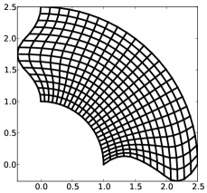
Figure 3: The FE-discretized domain covered by quadrilateral elements, forming the FE mesh.

Having the geometry discretized, a suitable approximation of the fields has to be devised. In (classical¹) FEM, the base functions with small support are polynomials, see Figure 4 for an illustration in 1D. A $k$-th base function is nonzero only in elements that share the DOF $T_{k}$ and it is a continuous polynomial over each element.

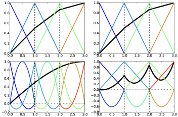
Figure 4: The 1D FE basis on three line elements with black thick line an interpolated function resulting from the same DOF vector for each row: top: linear, bottom: quadratic, left: Lagrange, right: Lobatto. Each basis function has a single color.

The thick black lines in Figure 4 result from interpolation of the DOF vector generated by $\sin(\frac{\pi}{2}\frac{x}{3})$ evaluated in points of maximum of each basis function. The left column of the figure shows the Lagrange polynomial basis, which is interpolatory, i.e., a DOF value is equal to the approximated function value in the point, called node, where the basis is equal to 1. The right column of the figure shows the Lobatto polynomial basis, that is not interpolatory for DOFs belonging to basis functions with order greater than 1 - that is why the bottom right interpolated function differs from the other cases. This complicates several things (e.g. setting of Dirichlet boundary conditions - a projection is needed), but the hierarchical nature of the basis, i.e. increasing approximation order means adding new basis functions without modifying the existing ones, has also advantages, for example better condition number of the matrix for higher order approximations.

The basis functions are usually defined in a reference element, and are then mapped to the physical mesh elements by an (affine) transformation. For our mesh we will use bi-quadratic polynomials over the reference quadrilateral - a quadratic function along each axis direction, such as those in the bottom row of Figure 4.

Several families of the element basis functions exist. In SfePy, Lagrange basis and Lobatto (hierarchical) basis can be used on quadrilaterals, see Figure 5.

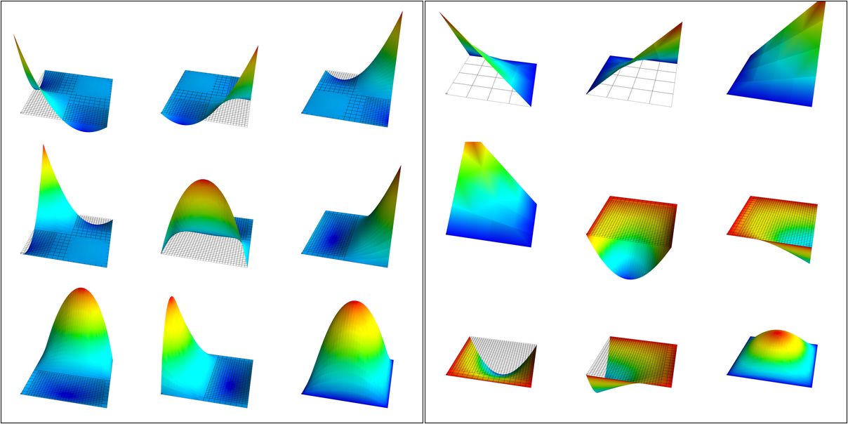
Figure 5: Bi-quadratic basis functions on the reference quadrilateral: left: Lagrange right: Lobatto.

3.2 IGA

In IGA, the CAD geometrical description in terms of NURBS patches is used directly for the approximation of the unknown fields, without the intermediate FE mesh - the meshing step is removed, which is one of its principal advantages. As described in Geometry Description using NURBS, a D-dimensional geometric domain is defined by

$$\underline{x}(\underline{\xi})=\sum_{A=1}^{n}\bm{P}_{A}R_{A,p}(\underline{\xi})=\bm{P}^{T}\bm{R}(\underline{\xi})\;,$$

where $\underline{\xi}=\{\xi_{1},\dots,\xi_{D}\}$ are the parametric coordinates, and $\bm{P}=\{\bm{P}_{A}\}_{A=1}^{n}$ is the set of control points. The same NURBS basis is used also for the approximation of PDE solutions. For our temperature problem we have

$$T(\underline{\xi})=\sum_{A=1}^{n}T_{A}R_{A,p}(\underline{\xi})\;,\quad s(\underline{\xi})=\sum_{A=1}^{n}s_{A}R_{A,p}(\underline{\xi})\;,$$

where $T_{A}$ are the unknown DOFs - coefficients of the basis in the linear combination, and $s_{A}$ are the test function DOFs.

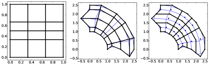
Figure 6: From left to right: parametric mesh (tensor product of knot vectors), control mesh, Bézier mesh.

Our domain in Figure 2 can be exactly described by a single NURBS patch. Several auxiliary grids (called "meshes" as well, but do not mistake with the FE mesh) can be drawn for the patch, see Figure 6. The parametric mesh is simply the tensor product of the knot vectors defining the parametrization - the lines correspond to the knot vector values. In our case there are four unique knot values in the first parametric axis and five in the second axis. The control mesh has vertices given by the NURBS patch control points and connectivity corresponding to the tensor product nature of the patch. The Bézier mesh will be described below. The thin blue lines are iso-lines of the NURBS parametrization, as in Figure 2.

On a single patch, such as our whole domain, the NURBS basis can be arbitrarily smooth - this is another compelling feature not easily obtained by FEM. The basis functions $R_{A,p}$, $A=1,\dots,n$ on the patch are uniquely determined by the knot vector for each axis, and cover the whole patch, see Figure 7.

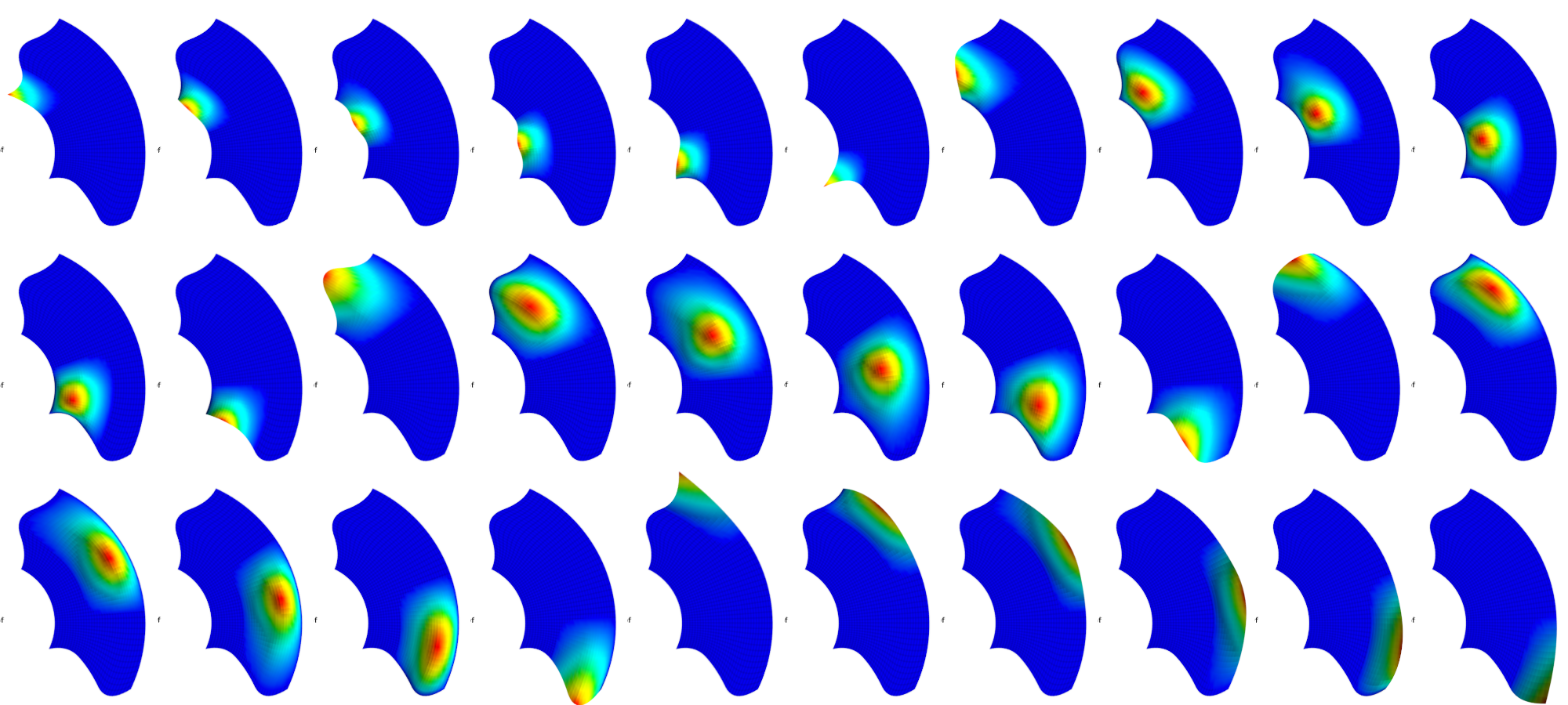
Figure 7: The degree 2 NURBS basis functions on the single patch domain.

4 IGA Implementation in SfePy

Our implementation uses a variant of IGA based on Bézier extraction operators [BE] that is suitable for inclusion into existing FE codes. The code itself does not see the NURBS description at all. The NURBS description can be prepared, for example, using igakit package, a part of [PetIGA].

The Bézier extraction is illustrated in Figure 8. It is based on the observation that repeating a knot in the knot vector decreases continuity of the basis in that knot by one. This can be done in such a way that the overall shape remains the same, but the "elements" appear naturally as given by non-zero knot spans. The final basis restricted to each of the elements is formed by the Bernstein polynomials $\bm{B}$.

In [BE] algorithms are developed that allow computing Bézier extraction operator $\bm{C}$ for each such element such that the original (smooth) NURBS basis function $\bm{R}$ can be recovered from the local Bernstein basis $\bm{B}$ using $\bm{R}=\bm{C}\bm{B}$. The Bézier extraction also allows construction of the Bézier mesh, see Figure 6, right. The code then loops over the Bézier elements and assembles local contributions in the usual FE sense.

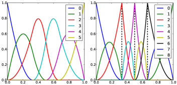
Figure 8: From left to right: NURBS basis of degree 2 that describes the second axis of the parametric mesh, corresponding Bernstein basis with Bézier elements delineated by vertical lines.

In SfePy, various subdomains can be defined using regions, see [SfePy]. For example, below we use the following region definition to specify an internal subdomain:

’vertices in (x > 1.5) & (y < 1.5)’

To make this work with IGA, where no real mesh exists, a topological Bézier mesh is constructed, using only the corner vertices of the Bézier mesh elements, because those are interpolatory, i.e., they are in the domain or on its boundary, see Figures 6, 8 right.

The regions serve both to specify integration domains of the terms that make up the equations and to define the parts of boundary, where boundary conditions are to be applied. SfePy supports setting the Dirichlet boundary conditions by user-defined functions of space (and time). To make this feature work with IGA, a projection of the boundary condition functions to the space spanned by the appropriate boundary basis functions was implemented.

4.1 Notes on Code Organization

Although the Bézier extraction technique shields the IGA-specific code from the rest of the FEM package, the implementation was not trivial. Similar to the Lobatto FE basis, the DOFs corresponding to the NURBS basis are not equal to function values with the exception of the patch corners. Moreover, the IGA fields do not work with meshes at all - they need the NURBS description of the domain together with the Bézier extraction operators and the topological Bézier mesh. So the original sfepy.fem sub-package was renamed and split into:

• sfepy.discrete for the general classes independent of the particular discretization technique (for example variables, equations, boundary conditions, materials, quadratures, etc.);

• sfepy.discrete.fem for the FEM-specific code;

• sfepy.discrete.iga for the IGA-specific code;

• sfepy.discrete.common for common functionality shared by some classes in sfepy.discrete.fem and sfepy.discrete.iga.

In this way, circular import dependencies were minimized.

4.2 Using IGA

As described in [SfePy], problems can be described either using problem description files - Python modules containing definitions of the various components (mesh, regions, fields, equations, …) using basic data types such as dict and tuple, or using the sfepy package classes directly interactively or in a script. The former way is more basic and will be used in the following.

In a FEM computation, a mesh has to be defined using:

filename_mesh = ’fe_domain.mesh’In an IGA computation, a NURBS domain has to be defined instead:

filename_domain = ’ig_domain.iga’where the ’.iga’ suffix is used for a custom HDF5 file that can be prepared by functions in sfepy.discrete.iga.

A scalar real FE field with the approximation order 2 called ’temperature’ can be defined by:

# Lagrange basis is the default.fields = {    ’temperature’ :    (’real’, 1, ’Omega’, 2),}# Lobatto basis.fields = {    ’temperature’ :    (’real’, 1, ’Omega’, 2, ’H1’, ’lobatto’),}An analogical IGA field can be defined by:

fields = {    ’temperature’ :    (’real’, 1, ’Omega’, None, ’H1’, ’iga’),}Here the approximation order is None, as it is given by the ’.iga’ domain file.

The above are the only changes required to use IGA - everything else remains the same as in FEM calculations. The scalar and vector volume terms (weak forms, linear or nonlinear) listed at http://sfepy.org/doc-devel/terms_overview.html can be used without modification.

4.3 Limitations

There are currently several limitations that will be addressed in future:

• projections of functions into the NURBS basis;

• support for surface integrals;

• linearization of results for post-processing;

  • currently the fields on a tensor-product patch are sampled by fixed parameter vectors and a corresponding FE-mesh is generated;

• all variables have to have the same approximation order, as the basis is given by the domain file;

• the domain is a single NURBS patch only.

5 Examples

Numerical examples illustrating the IGA calculations are presented below. The corresponding problem description files for SfePy (version 2014.3) can be downloaded from https://github.com/sfepy/euroscipy2014-iga-examples, revision 28b1fe9bff7043da6fd159c20b9f244337a17e82, or from http://dx.doi.org/10.5281/zenodo.12257.

5.1 Temperature Distribution

The 2D domain depicted in Figure 2 is used in this example. The temperature distribution is given by the solution of the Laplace equation (4) with a particular set of Dirichlet boundary conditions on $\Gamma_{D}$. The region $\Gamma_{D}$ consisted of two parts $\Gamma_{1}$, $\Gamma_{2}$ of the domain boundary on the opposite edges of the patch, see Figure 9 - the temperature was fixed to 0.5 on $\Gamma_{1}$ and to -0.5 on $\Gamma_{2}$, as can be seen in Figure 10. As mentioned in Limitations, the resulting field $T$ was sampled by fixed uniform parameter vectors along each axis, and the corresponding output FE mesh was generated. The mesh was saved in the VTK format and the results visualized using SfePy’s postproc.py script based on Mayavi. The generated mesh can be seen as the undeformed wire-frame.

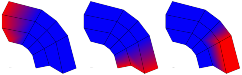
Figure 9: The regions defined on the domain shown on the topological Bézier mesh by red color. From left: $\Gamma_{1}$, $\Gamma_{2}$, $\Omega_{0}$

For comparison with a FEM solution, see Figure 11. The FEM problem had 1363 DOFs in the linear system, while the IGA problem only 20. The mesh depicted in Figure 3 was used for the FEM computation.

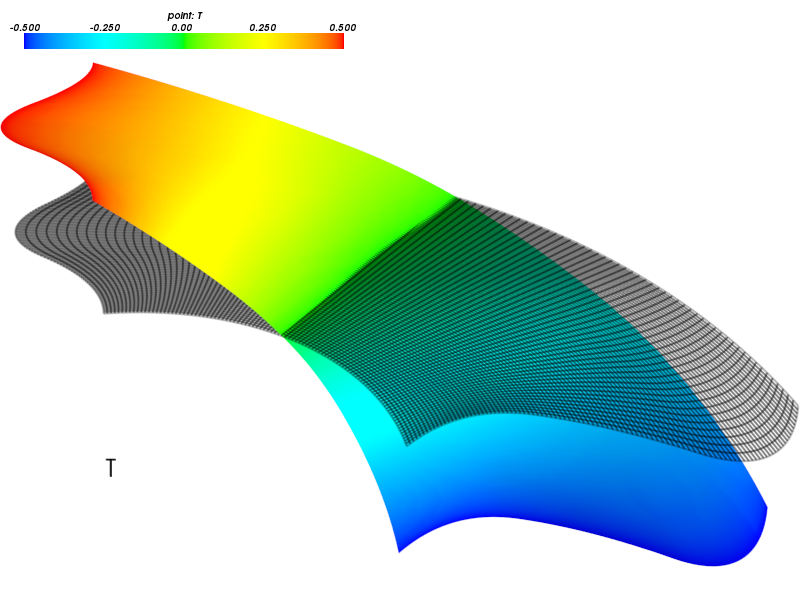
Figure 10: A solution of the 2D Laplace equation.

Figure 11: A solution of the 2D Laplace equation by FEM.

Next we added a negative source term to the Laplace equation in region $\Omega_{0}$ (see Figure 9 right) to obtain the Poisson equation:

$$\int_{\Omega}\nabla s\cdot\nabla T = \int_{\Omega_{0}}-2s\;,\quad\forall s\in H^{1}_{0}(\Omega)\;,$$ (7)

$$T = \bar{T}\quad\mbox{ on }\Gamma_{D}\;,$$ (8)

The corresponding solution can be seen in Figure 12. The boundary conditions stayed the same as in the previous case.

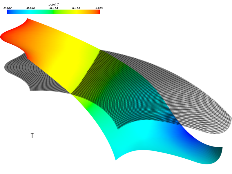
Figure 12: A solution of the 2D Poisson equation with volume source in a subdomain.

The complete problem description file for computing (7) is shown below. See [SfePy] or http://sfepy.org for explanation.

filename_domain = ’ig_domain.iga’regions = {    ’Omega’ : ’all’,    ’Omega_0’ : ’vertices in (x > 1.5) & (y < 1.5)’,    ’Gamma1’ : (’vertices of set xi10’, ’facet’),    ’Gamma2’ : (’vertices of set xi11’, ’facet’),}fields = {    ’temperature’    : (’real’, 1, ’Omega’, None, ’H1’, ’iga’),}variables = {    ’T’ : (’unknown field’, ’temperature’, 0),    ’s’ : (’test field’,    ’temperature’, ’T’),}ebcs = {    ’T1’ : (’Gamma1’, {’T.0’ : 0.5}),    ’T2’ : (’Gamma2’, {’T.0’ : -0.5}),}materials = {    ’m’ : ({’f’ : -2.0},),}integrals = {    ’i’ : 3,}equations = {    ’Temperature’    : """dw_laplace.i.Omega(s, T)       = dw_volume_lvf.i.Omega_0(m.f, s)"""}solvers = {    ’ls’ : (’ls.scipy_direct’, {}),    ’newton’ : (’nls.newton’, {        ’i_max’      : 1,        ’eps_a’      : 1e-10,    }),}

5.2 Elastic Deformation

This example illustrates a calculation with a vector variable, the displacement field $\underline{u}$, given by deformation of a 3D elastic body. The weak form of the problem is: Find $\underline{u}\in[H^{1}(\Omega)]^{3}$ such that:

$$\int_{\Omega}D_{ijkl}\ e_{ij}(\underline{v})e_{kl}(\underline{u}) = 0\;,\quad\forall\underline{v}\in[H^{1}_{0}(\Omega)]^{3}\;,$$

$$\underline{u} = \bar{\underline{u}}\quad\mbox{ on }\Gamma_{D}\;,$$

where $D_{ijkl}=\mu(\delta_{ik}\delta_{jl}+\delta_{il}\delta_{jk})+\lambda\delta_{ij}\delta_{kl}$ is the isotropic stiffness tensor given in terms of Lamé’s coefficients $\lambda$, $\mu$ and $e_{ij}(\underline{u})=\frac{1}{2}(\frac{\partial u_{i}}{\partial x_{j}}+\frac{\partial u_{j}}{\partial x_{i}})$ is the Cauchy, or small strain, deformation tensor. The equation expresses the internal and external (zero here) force balance, where the internal forces are described by the Cauchy stress tensor $\sigma_{ij}(\underline{u})=D_{ijkl}\ e_{kl}(\underline{u})$.

The 3D domain $\Omega$ was simply obtained by extrusion of the 2D domain of the previous example, and again $\Gamma_{D}$ consisted of two parts $\Gamma_{1}$, $\Gamma_{2}$. The body was clamped on $\Gamma_{1}$: $\underline{u}=0$ and displaced on $\Gamma_{2}$: $u_{1}=0.01$, $u_{2}(\underline{x})=-0.02x_{2}$ and $u_{3}(\underline{x})=-0.02+(0.15*(x_{1}-1)^{2})$, for $\underline{x}\in\Gamma_{2}$. Note that the Dirichlet boundary conditions on $\Gamma_{2}$ depend on the position $\underline{x}$. The corresponding solution can be seen in Figure 13.

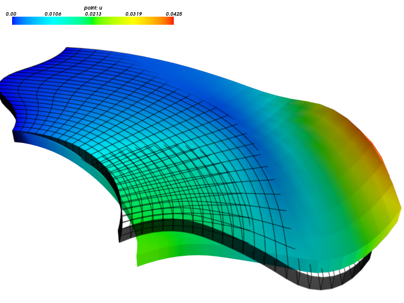
Figure 13: A solution of the 3D linear elasticity equation. The undeformed domain is shown as a wireframe, 10x magnified deformation.

6 Conclusion

Two numerical techniques for discretization of partial differential equations were briefly outlined and compared, namely the well-established and proven finite element method and its much more recent generalization, the isogeometric analysis, on the background given by the open source finite element package SfePy, that has been recently enhanced with the isogeometric analysis functionality.

The Bézier extraction operators technique, that was used for a relatively seamless integration into the existing finite element package, was mentioned, as well as some of the difficulties "on the road" and limitations of the current version.

Numerical examples - a scalar diffusion problem in 2D and a vector elastic body deformation problem in 2D were shown.

6.1 Support

Work on SfePy is partially supported by the Grant Agency of the Czech Republic, project P108/11/0853.

References

- [FEM] Thomas J. R. Hughes, The Finite Element Method: Linear Static and Dynamic Finite Element Analysis, Dover Publications, 2000.
- [IGA] J. Austin Cottrell, Thomas J.R. Hughes, Yuri Bazilevs. Isogeometric Analysis: Toward Integration of CAD and FEA. John Wiley & Sons. 2009.
- [NURBS] Les Piegl & Wayne Tiller: The NURBS Book, Springer-Verlag 1995–1997 (2nd ed.).
- [BE] Michael J. Borden, Michael A. Scott, John A. Evans, and Thomas J.R. Hughes: Isogeometric Finite Element Data Structures based on Bezier Extraction of NURBS, Int. J. Numer. Meth. Engng., 87: 15–47. doi: 10.1002/nme.2968, 2011.
- [PetIGA] N. Collier, L. Dalcin, V.M. Calo: PetIGA: High-Performance Isogeometric Analysis, arxiv 1305.4452, 2013, http://arxiv.org/abs/1305.4452.
- [SfePy] Robert Cimrman: SfePy - Write Your Own FE Application, arxiv 1404.6391, 2014, http://arxiv.org/abs/1404.6391.