SClib, a hack for straightforward embedded C functions in Python

Abstract

We present SClib, a simple hack that allows easy and straightforward evaluation of C functions within Python code, boosting flexibility for better trade-off between computation power and feature availability, such as visualization and existing computation routines in SciPy.

We also present two cases were SClib has been used.

In the first set of applications we use SClib to write a port to Python of a Schrödinger equation solver that has been extensively used the literature, the resulting script presents a speed-up of about 150x with respect to the original one. A review of the situations where the speeded-up script has been used is presented. We also describe the solution to the related problem of solving a set of coupled Schrödinger-like equations where SClib is used to implement the speed-critical parts of the code. We argue that when using SClib within IPython we can use NumPy and Matplotlib for the manipulation and visualization of the solutions in an interactive environment with no performance compromise.

The second case is an engineering application. We use SClib to evaluate the control and system derivatives in a feedback control loop for electrical motors. With this and the integration routines available in SciPy, we can run simulations of the control loop a la Simulink. The use of C code not only boosts the speed of the simulations, but also enables to test the exact same code that we use in the test rig to get experimental results. Again, integration with IPython gives us the flexibility to analyze and visualize the data.

1 Introduction

Embedding code written in oder languages is a common theme in the Python context, the main motivation being speed boosting. Several alternatives exist to achieve this, such as Cython [Cython], CFFI [CFFI], SWIG [SWIG], weave [weave], among others. We present yet another alternative, which may be quite close to CFFI than to the others. The motivation to write SClib grew out of the urge to integrate C code, which was already written, into the Python environment, minimizing the intervention of the code. Part of the resulting work is briefly introduced later, in the engineering application section.

Nevertheless, embedding compiled code in Python will naturally have an impact in performance, for instance, when the compiled code takes care of computer intensive numerics. The first application we introduce (in particle physics), leverages SClib in this sense, outsourcing the numerics to the compiled code and using the Python environment for visualization.

2 SClib

At the core of SClib¹ is ctypes [Hell], which actually does the whole work: it maps Python data to C compatible data and provides a way to call functions in DLLs or shared libraries. SClib acts as glue: it puts things together for the user, to provide him with an easy to use interface.

The requirements for SClib are very simple: call a function on an array of numbers of arbitrary type and size and return the output of the function, again of arbitrary type and size.

The resulting interface is also very simple: A library is initialized in the Python side with the path to the DLL (or shared library) and a list with the names of the functions to be called:

In [1]: import SClib as scIn [2]: lib = sc.Clib(’test.so’, [’fun’])The functions are then available as members of the library and can be called with the appropriate number of arguments, which are one dimensional arrays of numbers. The function returns a list containing the output arrays of the function:

In [3]: out, = lib.fun([0])In the C counterpart, the function declaration must be accompanied with specifications of the inputs and outputs lengths and types. This is accomplished with the helper macros defined in sclib.h:

#include <sclib.h>SCL_OL(fun, 1,   1);   /* outputs lengths */SCL_OT(fun, 1, INT);   /* outputs types */SCL_IL(fun, 1,   1);   /* inputs lengths */SCL_IT(fun, 1, INT);   /* inputs types */void fun(int * out, int * in) {    *out = 42;}An arbitrary number of inputs or outputs can be specified, for example:

#include <math.h>#include <sclib.h>SCL_OL(fun, 2,   1,     2);SCL_OT(fun, 2, INT, FLOAT);SCL_IL(fun, 2,   1,     2);SCL_IT(fun, 2, INT, FLOAT);void fun(int * out0, float * out1,         int * in0, float * in1) {    *out0 = 42*in0[0];    out1[0] = in1[0]*in1[1];    out1[1] = powf(in1[0], in1[1]);}In the function declaration, all the outputs must precede the inputs and must be placed in the same order as in the SCL macros.

These specifications are processed during compilation time, but only the number of inputs and outputs is static, the lengths of each component can be overridden at run time:

In [4]: lib.INPUT_LEN[’fun’] = [10, 1]In [5]: lib.retype()In these use cases the length of the arguments should be given to the function through an extra integer argument.

In the function body, both inputs and outputs should be treated as one dimensional arrays.

3 Application in Quarkonium Physics

3.1 Motivation

The Schrödinger equation is the fundamental equation for describing non-relativistic quantum mechanical dynamics. For the applications we will present in this section we will focus on the time-independent version which, in natural units, is given by

$$\left(-\frac{\nabla_{\mathbf{r}}^{2}}{2\mu}+V(\mathbf{r})\right)\psi(\mathbf{r})=E\psi(\mathbf{r}).$$ (1)

It corresponds to an eigenvalue equation where the term inside the parenthesis in l.h.s. is called the Hamiltonian operator, the value $E$, its eigenvalue, is the measurable quantity (the energy) associated with it, $\mu$ is the reduced mass of the system (it correspond the mass of the particle in one-particle systems) and the wavefunction, $\psi(\mathbf{r})$ is the entity containing all the information about the system, since its modulus squared correspond to the probability density of a given measurement, it has to be normalized to unity. The term $V({\mathbf{r}})$ in the Hamiltonian is called the potential.

Since its discovery, the Schrödinger equation has played an important role in our understanding of nature and it is present in almost every aspect of modern physics. In this section we will review some cases where SClib has been used to implement solutions of the computing problems associated with eq. (1) that arise in the study of heavy quarkonia².

Quarkonium is a bound-state composed by a quark and its corresponding antiquark. By heavy we mean states composed by charm and bottom quarks, called charmonium and bottomonium respectively. Due to its large mass, the top quark decays before forming a bound state. In heavy quarkonium the relative velocity between the quark and antiquark inside of the bound-system is believed to be small enough for the system to be considered, at least in a first approximation, non-relativistic, making it suitable for being described by eq. (1). Considering the equal mass case with a spherically symmetric potential the angular part can be neglected (it correspond to the spherical harmonics) and the relevant part of eq. (1) reduces to the one-dimensional equation given by

$$\left[-\frac{1}{m}\frac{d^{2}}{dr^{2}}+\frac{l(l+1)}{mr^{2}}+V(r)\right]y_{n,l}(r)=E_{n,l}y_{n,l}(r),$$ (2)

where $r$ is the relative distance between the quark and the antiquark, $l$ is the angular momentum quantum number, $m$ is the (anti)quark mass (for equal mass $2\mu=m$), $y_{n,l}$ is called the reduced wavefunction and the eigenvalue $E_{n,l}$ is interpreted as the binding energy of the bound-system, where $n=0,1,2,\dots$ accounts for the number of nodes (radial excitations) of the wavefunction. The mass of the quarkonium is then given by

$$M=2m+E_{n,l}.$$ (3)

The potential $V(r)$ describes the quark-antiquark interaction, it is a function of $r$ and $\Lambda_{\rm QCD}$, the typical hadronic scale ($\sim 200\,{\rm MeV}$). For $r\Lambda_{\rm QCD}\ll 1$ (short-distance regime) the potential may be evaluated perturbatively, but for $r\Lambda_{\rm QCD}\sim 1$ (long-distance regime) it cannot. To overcome this issue, models based on non-relativistic reductions of phenomenological observations have been used to describe heavy quarkonia, one these being the so-called Cornell potential [Eich74], [Eich78], [Eich79]

$$V(r)=\frac{a}{r}+kr,$$ (4)

where $a$ and $k$ are parameters which need to be fixed by experimental (or lattice) data of some observable. This potential incorporates two of the main observed characteristics of the quark-antiquark interaction: at short distances it exhibits a Coulombic behavior and in the long-distance regime the interaction is dominated by a confinement phase.

Since the beginning of the last decade, non-relativistic effective field theories (EFT), in particular non-relativistic QCD (NRQCD) [Cas85], [Bod94] and potential NRQCD (pNRQCD) [Bra99], have become the state-of-the-art tools for the study of heavy quarkonia (for review see [Bra04]). NRQCD is obtained from QCD integrating out modes that scale like $m$, while pNRQCD is obtained from NRQCD integrating out modes that scale like the quark momentum³.

The physics of the modes that have been integrated out is encoded in Wilson coefficients that must be calculated comparing at the same scale the results (observables, Green functions) of the EFT, with the ones of QCD (for NRQCD) or NRQCD (for pNRQCD). A key feature of pNRQCD is that it allows the relativistic corrections to the quark-antiquark potential to be organized as an expansion in powers of $1/m$. Up to second order $V(r)$ can be written as

$$V(r)=V^{(0)}(r)+\frac{V^{(1/m)}(r)}{m}+\frac{V^{(1/m^{2})}(r)}{m^{2}},$$ (5)

where $V^{(1/m)}$ and $V^{(1/m^{2})}$ are derived from QCD through the matching procedure with NRQCD. The details about $V^{(1/m)}$ and $V^{(1/m^{2})}$ and how they are obtained are beyond the scope of this document, however, we can list some of their features:

• They correspond to correlators that in the short-distance regime can be computed in perturbation theory.

• In the long-distance regime they can be computed in lattice QCD, however only some of these correlators have been calculated.

• Eq. (4) correspond, at least qualitatively, to the leading order $V^{(0)}$ in eq. (5)

For the details about the derivation of the terms present in eq. (5) we refer the reader to [Bra00] and [Pin00]. It is important to recall that, although it can not be evaluated analytically in the whole range of $r$, eq. (5) represents a model-independent expression for the quark-antiquark potential, contrary to models like the one presented in eq. (4).

Using perturbation theory to include the relativistic corrections to the potential, the expression for the bound-state mass reads

$$M = 2m+E_{n,l}^{(0)}+\frac{\langle nl|V^{(1/m)}(r)|nl\rangle}{m}$$

$$+ \frac{\langle nl|V^{(1/m^{2})}(r)|nl\rangle}{m^{2}}+\frac{1}{m^{2}}\sum_{m\neq n}^{\infty}\frac{|\langle nl|V^{(1/m)}|ml\rangle|^{2}}{E_{n,l}^{(0)}-E_{ml}^{(0)}},$$

where $E_{il}^{(0)}$ comes from solving eq. (2) with $V(r)=V^{(0)}(r)$ and

$$\langle nl|f(r)|n^{\prime}l^{\prime}\rangle\propto\int_{0}^{\infty}dr\,y_{n,l}(r)f(r)y_{n^{\prime}l^{\prime}}(r),$$

where the proportionality factor will depended on the corresponding quantum numbers of the operators appearing in $V^{(1/m)}$ and $V^{(1/m^{2})}$.

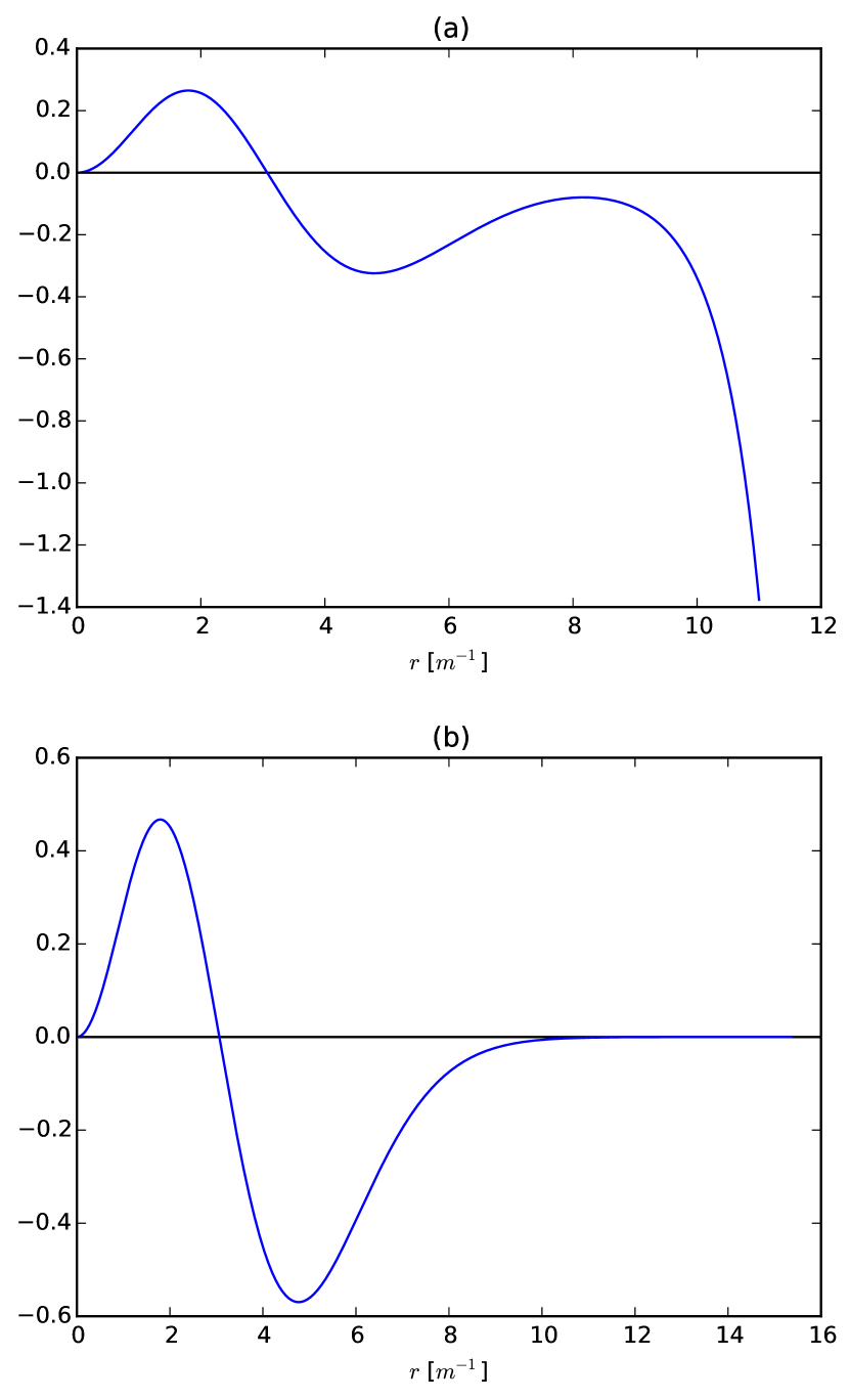
Figure 1: Reduced wavefunctions $y_{n,l}(r)$ for two steps in the search of the eigenvalue $E_{n=1\,l=1}$. For each step in the process to find the eigenvalue the nodes of the $y_{n,l}$ are counted, only when the value of $E_{n,l}$ corresponds to an eigenvalue $y_{n,l}$ is not divergent. In the plot (a) $E_{n,l}=3.1\,m$ and $y_{n,l}$ fulfills the condition of having one node, however, the accuracy in the value of $E_{n,l}$ is too low and the function diverges. In the plot (b) $E_{n,l}=3.10952\,m$ so $y_{n,l}\rightarrow 0$ for larger values of $r$. We have used the Cornell potential eq. (4) with parameters $m=1$ $a=0.1$, $k=0.5m^{2}$, all dimensions defined in terms of the mass.

3.2 Applications of SClib

The simplest computational problem related to eq. (2) is to find $E_{n,l}$ for a given $n$ and $l$. Methods to solve this problem have been implemented since long ago (see for instance [Fal85]), in a nutshell, the standard method consist of applying two known constraints to the reduced wavefunction $y_{n,l}$:

• The number of nodes of $y_{n,l}(r)$ must be equal to $n$.

• $y_{n,l}(r)$ has to be normalizable

$$\int_{0}^{\infty}dr[y_{n,l}(r)]^{2}=1.$$ (7)

In general $y_{n,l}(r)$ will diverge except when $E_{n,l}$ corresponds to an eigenvalue. The procedure to find the eigenvalue consists in to perform a scan of values of $E_{n,l}$ until $y_{n,l}(r)$ has $n$ nodes and converges for a large enough value of $r$ (see Fig. 1). This implies that for each test value of $E_{n,l}$ eq. (2) must be (numerically) solved. A popular⁴ Mathematica [Mat9] implementation of this method has been available in [Luc98]. This script has the advantage that the user can profit from the Mathematica built-in functions to plot, integrate or store the resulting wavefunctions, however, it has a very poor performance. With the goal of mimicking some of the advantages of this script, but without compromising speed, we ported the algorithm in [Luc98] to Python. The resulting script, SChroe.py⁵, uses SClib to implement the speed-critical parts of the algorithm. In Schroe.py the wavefunctions are stored as NumPy arrays [NumPy] so when the script is run within IPython [IPy] together with SciPy [SciPy], NumPy and Matplotlib [Mplot] the user can profit of the same or more flexibility as with the Mathematica script plus a boosted speed. In table 1 we compare the performance of SChroe.py against other implementations of the same algorithm⁶.

$n$	$E_{n,l=1}\,\,[m]$	schroe.nb [Luc98]	Python	SChroe.py
0	2.15789	98.88	25.46	0.66
1	3.10952	124.14	30.95	0.75
2	3.93850	135.68	35.32	0.84
20	13.5995	370.0	88.04	1.99

TABLE II: Time in seconds taken to compute the eigenvalues and reduced wavefunctions for the Cornell potential eq. (4). The column Python correspond to the implementation of the algorithm in Python without SClib. The parameters of the potential are the same as in Fig. 1. All the scripts were tested in the same machine, a notebook with a 2.4 Ghz core i5 processor (dual core) and 8 GB of RAM.

In [Bra14] SChroe.py has been used to evaluate the relativistic corrections to the mass spectrum of quarkonium in the long-distance regime. In that paper the relativistic corrections $V^{(1/m)}$ and $V^{(1/m^{2})}$ appearing in (3.1) were evaluated assuming the hypothesis that in the long-distance regime the interaction between the quark and the antiquark can be described by a string. In Fig. 2 we show some of the energy levels (masses) corresponding to the string spectrum. It is noteworthy to mention that all the numerical calculations and plots of that paper were done with IPython using the SciPy library.

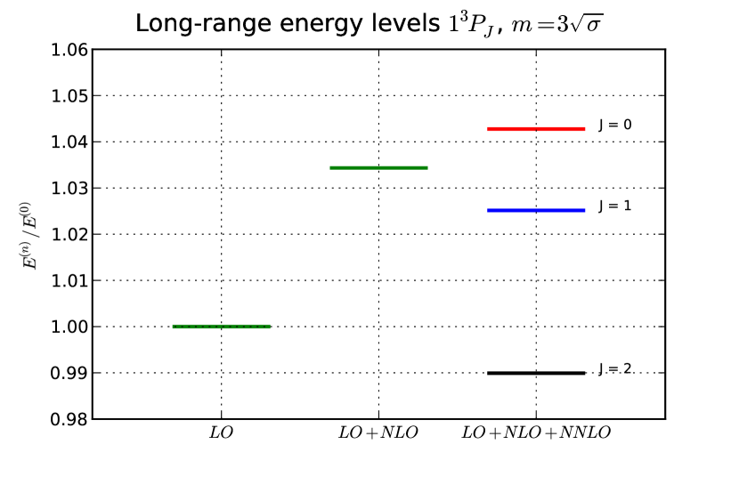
Figure 2: Long-range energy levels of the first triplet quarkonium state. The lines are calculated from eq. (3.1) using the relativistic corrections derived from the string hypothesis [Bra14a]. The leading order (LO) correspond to eq. (4) setting $a=0$ and $k=1$ (in the plot labeled $\sigma$) and $m=3\sqrt{k}$. This plot shows the relative size of the next-to-leading-order (NLO) correction (the term proportional to $1/m$ in the r.h.s. of eq. (3.1)) and the newly computed next-to-next-to-leading-order (NNLO) corrections (the terms proportional to $1/m^{2}$). For more details see [Bra14a].

An application in which the speed of SChroe.py plays an important role is fixing the parameters of the potential given some experimental input. For instance, consider the problem of finding the parameters $a$ and $k$ of eq. (4) together with $m$, given the experimental values of the masses of three different quarkonium states. If relativistic corrections are included, in order to find the parameters we must solve a system of three equations like eq. (3.1). For each probe value of $(a,k,m)$ we have to find the eigenvalues and reduced wavefunctions of eq. (2) and then with these values evaluate the sums and integrals in (3.1). A parameter fixing of this type was necessary to implement in [Bra14b]. The implementation has been carried out using SChroe.py together with a mixture of C and SciPy functions using SClib to link both environments⁷.

Another related computational problem that arises from the study of heavy quarkonium hybrids, bound-states composed by a quark-antiquark pair plus an exited gluon, is to solve a system of $N$ Schrödinger-like coupled equations. Explicitly the system to solve reads

$$\left(-\frac{\delta_{ij}}{m}\frac{d^{2}}{dr^{2}}+V_{ij}(r,l)\right)u_{j,(n,l)}(r)=E_{n,l}\,u_{i,(n,l)}(r),$$ (8)

where $i=1,2,..N$ and the angular momentum dependence has been included in the potential matrix. A method to solve this equation for the case $N=2$ has been implemented in [Ber14]. The method relies on an extension of the nodal theorem [Ama95] and convergence conditions for the components of the vector wavefunction $u_{j,(n,l)}(r)$. The extension of the nodal theorem states that the number of nodes of the determinant of the matrix $U_{n,l}(r)$, whose columns are $N$ lineal-independent solutions of eq. (8), is equal to $n$. The procedure then consist in a scan of values $E_{n,l}$; in each step the set of equations (8) is solved and the nodes of $|U_{n,l}(r)|$ are counted for a large enough interval of $r$. As in the one-dimensional case, if $E_{n,l}$ approached to an eigenvalue the components of $u_{j,(n,l)}$ converge for large $r$. In the solution presented in [Ber14] the performance-intensive parts of the implementation rely on C functions linked to the IPython interface trough SClib.

As an example of the application of the method implemented in [Ber14], in Fig. 3 we show the results for the search of the first two eigenvalues and wavefunctions with the matrix potential given by

$$V_{ij}(r,l)=\begin{pmatrix}\frac{l(l+1)+2}{mr^{2}}+F_{0}(r)&-\frac{2\sqrt{l(l+1)}}{mr^{2}}\\ -\frac{2\sqrt{l(l+1)}}{mr^{2}}&\frac{l(l+1)}{mr^{2}}+F_{1}(r)\end{pmatrix}$$ (9)

where

$$F_{i}(r)=\ln(a_{i}+b_{i}r).$$

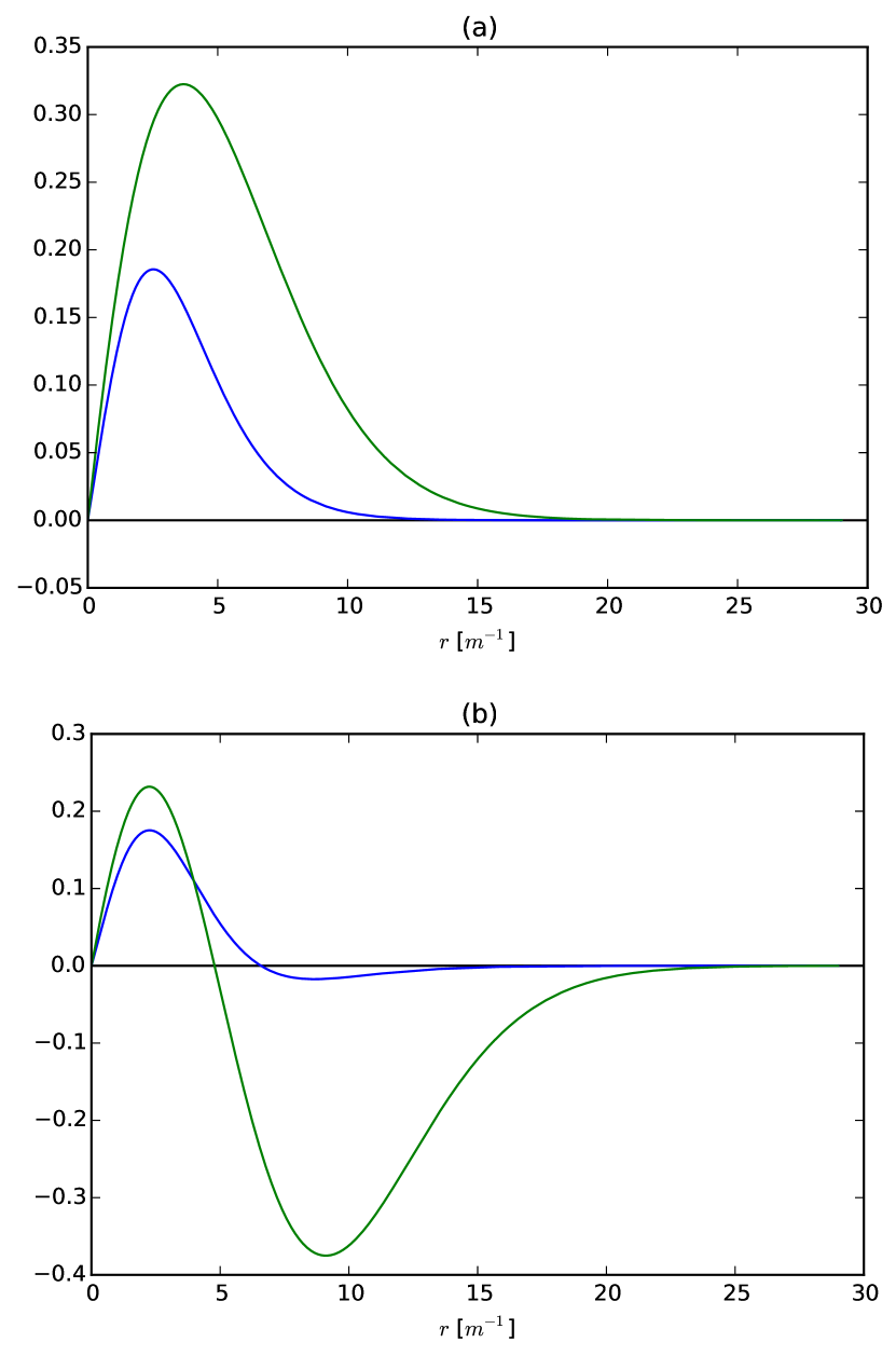
Figure 3: Solutions for the components of the vector wavefunction $u_{n,l}(r)$ for the first two eigenvalues ($l=1$) of eq. (8) with the matrix potential given in (9). We have used $m=1$, $a_{0}=1$, $b_{0}=0.5$, $a_{1}=2$ and $b_{1}=0.1$. The eigenvalues are $E_{n=0,l=1}=1.01727\,m$ for Fig. (a) and $E_{n=1,l=1}=1.18789\,m$ for Fig. (b).

In all the applications described in this section the combination of SClib and the SciPy library within an interactive environment like IPython provided a powerful framework based entirely on open source software for solving problems that require a high performance and visualization tools.

4 Application in Control Engineering

Figure 4: General scheme of a control system.

Most control systems have the structure depicted in Fig 4. $G$ is the plant, it represent the natural phenomena we wish to control. We usually describe it using ordinary differential equations:

$$G:\;\left\{\begin{array}[]{rl}\frac{dx}{dt}&=f(x,u,d)\\ y&=c(x,u,d).\end{array}\right.$$ (10)

$x$ represents the internal state of the plant and $y$ its output (the measurements). $d$ is an independent variable, usually not measurable, named the perturbation and $u$ is the actuation: the degree of freedom used by the controller $C$ to achieve the control goal $r$. In general the controller is a function of the measurements and the reference $r$:

$$C:\;u=\pi(y,r),$$

but it also may comprise internal states. They are commonly used to reconstruct the state $x$ out of the history of $y$ and $u$. The latter systems are called state observers and the whole is called feedback control.

We use SClib to put together a simulator for these kind of systems. Both the system derivatives $f(\cdot)$ and the control $\pi(\cdot)$ are written in C and are evaluated using SClib. As stated before, the system state represents a natural phenomena, therefore it is natural to describe it as a continuous time variable, as eq. (10) suggests. To calculate the system state we have to solve this equation. In our simulator this is achieved using numerical methods, namely the integration routines available in scipy.integrate. On the other hand, the controller is usually implemented in a real-time computer, which can only sample $y$ at a fixed interval (called $h$): it is a discrete-time system. This means, that the simulator only needs to evaluate $\pi(\cdot)$ at given times.

Traditional controllers took the form of linear filters, which could even be implemented using analog circuitry. As control techniques and requirements advance, more complex controllers are devised. Many modern control techniques are based on optimization methods. Time-optimal controllers, for example, require the solution of an usually very complex optimization problem, to find a control $u$ that leads the system state $x$ towards its target $r$ in minimum time [Gru11]:

$$u^{*}=\pi^{*}(x)=\underset{\pi\in U,\,x\in X}{\operatorname{argmin}}\left\{T_{x}(u)\right\}.$$ (11)

Here $T_{x}(u)$ is the time required to lead $x$ towards its target and $X$ and $U$ are the regions where we want $x$ and $u$ to be confined, they constitute the constraints for the control problem. These kind of controllers require exhaustive computation and it is natural to implement them in C.

For motivation, we present the results for a minimum-time control strategy for a relatively simple and well known problem, the double integrator [Fu13]:

$$\frac{d}{dt}\left[\begin{array}[]{c}x_{0}\\ x_{1}\end{array}\right]=\left(\begin{array}[]{c}\nicefrac{{u}}{{\tau_{0}}}\\ \nicefrac{{x_{0}}}{{\tau_{1}}}\end{array}\right).$$ (12)

The relevance of this system lays in that it models many mechanical systems: $u$, $x_{0}$ and $x_{1}$ may represent acceleration, speed and position, for example.

Fig. 5 presents a minimum time control strategy for this system.

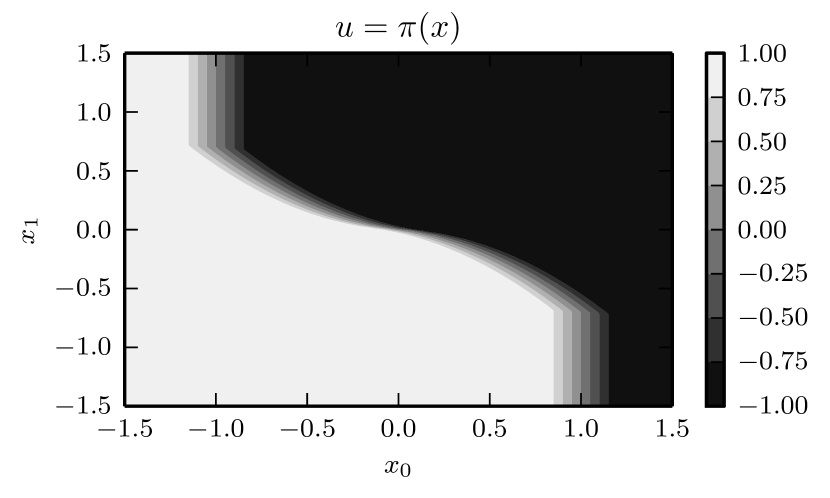
Figure 5: Time optimal control for the double integrator considering $\tau_{0}=\tau_{1}=5$, $u\in[-1,1]$, $h=1$ and $x\in[-1,1]\times\mathbb{R}$.

The form of $\pi(x)$ for this case reveals its non-linear nature.

Fig. 6 presents the trajectory developed by the state using this control strategy and random initial conditions.

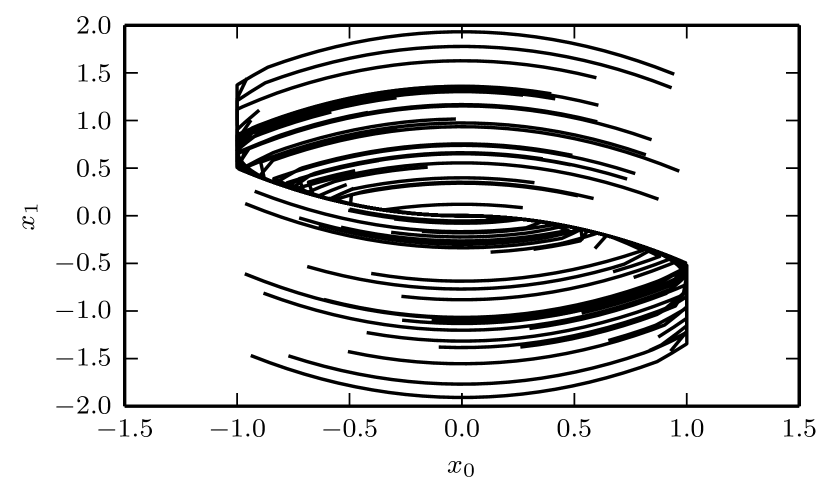
Figure 6: Time optimal trajectories for the double integrator, with random initial conditions.

These results were obtained using SClib and the devised simulator. The example code provided with SClib is ready to reproduce them.

The main advantage we obtained from this work was that, since we were using a Linux based real time system in our test rig, we could use exactly the same code for the simulations and the experimental tests. Another feature of this work is that it effectively replaces Simulink in all of our use cases using only free software.

5 Final Remark

We hope the applications of SClib scope beyond the ones listed in this paper since we believe it provides a simple but powerful way to boost Python performance.

6 Acknowledgments

H.M. acknowledges financial support from DAAD and the TUM Graduate School during the realization of this work.

References

- [Cython] Stefan Behnel, Robert Bradshaw, Lisandro Dalcín, Mark Florisson, Vitja Makarov, Dag Sverre Seljebotn. Cython is an optimising static compiler for both the Python programming language and the extended Cython programming language (based on Pyrex). http://www.cython.org/
- [CFFI] Armin Rigo and Maciej Fijalkowski C Foreign Function Interface for Python. http://cffi.readthedocs.org/en/release-0.8/
- [SWIG] SWIG developers. SWIG: Simplified Wrapper and Interface Generator http://swig.org/
- [weave] Ralf Gommers. Weave provides tools for including C/C++ code within Python code. https://github.com/scipy/weave
- [Hell] Heller. The ctypes module., https://docs.python.org/3.4/library/ctypes.html#module-ctypes
- [Bra14] N. Brambilla, S. Eidelman, P. Foka, S.Gardner, A. S. Kronfeld, M. G. Alford, R. Alkofer and M. Butenschoen et al., QCD and Strongly Coupled Gauge Theories: Challenges and Perspectives arXiv:1404.3723
- [Eich74] E. Eichten, K. Gottfried, T. Kinoshita, J. B. Kogut, K. D. Lane and T. M. Yan, The Spectrum of Charmonium, Phys. Rev. Lett. 34 , 369 (1975) Erratum-ibid. 36 , 1276 (1976)
- [Eich78] E. Eichten, K. Gottfried, T. Kinoshita, K. D. Lane and T. M. Yan, Charmonium: The Model, Phys. Rev. D 17 , 3090 (1978) Erratum-ibid. D 21 , 313 (1980)
- [Eich79] E. Eichten, K. Gottfried, T. Kinoshita, K. D. Lane and T. M. Yan, Charmonium: Comparison with Experiment, Phys. Rev. D 21 , 203 (1980).
- [Cas85] W. E. Caswell and G. P. Lepage, Effective Lagrangians for Bound State Problems in QED, QCD, and Other Field Theories, Phys. Lett. B 167 , 437 (1986).
- [Bod94] G. T. Bodwin, E. Braaten and G. P. Lepage, Rigorous QCD analysis of inclusive annihilation and production of heavy quarkonium, Phys. Rev. D 51 , 1125 (1995) Erratum-ibid. D 55 , 5853 (1997)
- [Bra04] N. Brambilla, A. Pineda, J. Soto and A. Vairo, Effective field theories for heavy quarkonium, Rev. Mod. Phys. 77 , 1423 (2005)
- [Bra99] N. Brambilla, A. Pineda, J. Soto and A. Vairo, Potential NRQCD: An Effective theory for heavy quarkonium, Nucl. Phys. B 566 , 275 (2000)
- [Bra00] N. Brambilla, A. Pineda, J. Soto and A. Vairo, The QCD potential at O(1/m), Phys. Rev. D 63 , 014023 (2001)
- [Pin00] A. Pineda and A. Vairo, The QCD potential at O(1/m^2): Complete spin dependent and spin independent result, Phys. Rev. D 63 , 054007 (2001) Erratum-ibid. D 64 , 039902 (2001)
- [Fal85] P. Falkensteiner and H. Grosse and F. Schoeberl and P. Hertel Comput. Phys. Comm. 34 , 287 (1985)
- [Luc98] W. Lucha and F. F. Schoberl, Solving the Schrödinger equation for bound states with Mathematica 3.0, Int. J. Mod. Phys. C 10 , 607 (1999)
- [dftatom] Čertík, O., Pask, J. E., Vackář, J. (2013). dftatom: A robust and general Schrödinger and Dirac solver for atomic structure calculations. Computer Physics Communications, 184(7), 1777–1791.
- [Mat9] Wolfram Research, Inc. Mathematica Version 9.0 (2012)
- [Bra14a] N. Brambilla, M. Groher, H. E. Martinez and A. Vairo, Effective string theory and the long-range relativistic corrections to the quark-antiquark potential, arXiv:1407.7761
- [Bra14b] N. Brambilla, H. E. Martinez and A. Vairo, TUM-EFT 40/13, In preparation.
- [SciPy] Eric Jones and Travis Oliphant and Pearu Peterson and others http://www.scipy.org/ (2001–)
- [NumPy] Stefan van der Walt, S. Chris Colbert and Gaël Varoquaux. The NumPy Array: A Structure for Efficient Numerical Computation, Computing in Science & Engineering, 13 , 22-30 (2011)
- [Ber14] M. Berwein and H. E. Martinez, TUM-EFT 48/14, In preparation.
- [Ama95] H. Amann and P. Quittner, A nodal theorem for coupled systems of Schrödinger equations and the number of bound states, Journal of Mathematical Physics 36 , 4553 (1995), doi:10.1063/1.530907.
- [Mplot] John D. Hunter. Matplotlib: A 2D Graphics Environment, Computing in Science & Engineering, 9 , 90-95 (2007)
- [IPy] Fernando Perez and Brian E. Granger. IPython: A System for Interactive Scientific Computing, Computing in Science & Engineering, 9 , 21-29 (2007)
- [Gru11] L. Gruene and J. Pannek, Nonlinear Model Predictive Control: Theory and Algorithms, Springer-Verlag, 2011.
- [Fu13] E. Fuentes, D. Kalise, J. Rodriguez, and R. Kennel Cascade-free predictive speed control for electrical drives, Industrial Electronics, IEEE Transactions on , vol. PP, no. 99, pp. 1–1, 2013.