Macroscopic (and Microscopic) Massless Modes

Abstract

We study certain spinning strings exploring the flat directions of $AdS_{3}\!\times\!S^{3}\!\times\!S^{3}\!\times\!S^{1}$, the massless sector cousins of $su(2)$ and $sl(2)$ sector spinning strings. We describe these, and their vibrational modes, using the $D(2,1;\alpha)^{2}$ algebraic curve. By exploiting a discrete symmetry of this structure which reverses the direction of motion on the spheres, and alters the masses of the fermionic modes $s\to\kappa-s$, we find out how to treat the massless fermions which were previously missing from this formalism. We show that folded strings behave as a special case of circular strings, in a sense which includes their mode frequencies, and we are able to recover this fact in the worldsheet formalism. We use these frequencies to calculate one-loop corrections to the energy, with a version of the Beisert–Tseytlin resummation.

1 Introduction

One of the new features of the integrable AdS₃/CFT₂ correspondence is the presence of massless modes in the BMN spectrum [1]. Each mode corresponds to a direction away from the string’s lightlike trajectory, and its mass is related to the radius of curvature of in this direction. In $AdS_{5}\!\times\!S^{5}$ all radii and all masses are equal, but in $AdS_{4}\!\times\!CP^{3}$ there are two distinct radii, and $AdS_{3}\!\times\!S^{3}\!\times\!S^{3}\!\times\!S^{1}$ four: the two 3-spheres are $1/\cos\upphi$ and $1/\sin\upphi$ times the $AdS$ radius (where $\upphi$ is an adjustable parameter). The flat $S^{1}$ direction, $u$, gives one massless boson, but the more interesting one arises from a combination of the equators of the two $S^{3}$ factors, $\uppsi$.

While there is no particular difficulty about treating the massless modes in the worldsheet language [6, 7], they have until recently been missing from the integrable description: they do not appear in the Bethe equations of [8], the S-matrix of [9] and the unitarity methods of [10, 11], nor the coset description of [12]. Recent progress on this problem (and the related one in $AdS_{3}\!\times\!S^{3}\!\times\!T^{4}$) has been reported in [13, 14, 15, 16], and we build on the work of Lloyd and Stefański [14] who studied the problem of how to incorporate the $\uppsi$ direction in the algebraic curve. This formalism maps the string to a Riemann surface, given by the log of the eigenvalues of the monodromy matrix [17, 18, 19, 20]. And what they showed is that the traditional way in which the Virasoro constraint was imposed here (as a condition on the residues of the quasimomenta at $x=\pm 1$) is too strong: it is not implied by the worldsheet Virasoro constraint when the target space has more than two factors. By loosening this restriction they were able to study some classical string solutions (with oscillatory $\uppsi$) which were previously illegal.

What the algebraic curve formalism has proven extremely useful for, and what we will use it for here, is working out the frequencies of vibrational modes (especially fermionic modes) of various macroscopic classical string solutions. The most important examples have been circular [21, 22, 23, 24, 25, 26, 27, 28] and folded [29, 30, 31, 32, 33, 34, 35, 36] spinning strings, described by one- or two-cut resolvents. The frequencies of these modes can be added up to give the one-loop correction to the energy, and this can be efficiently done using the algebraic curve [39, 40, 41, 33]. The $D(2,1;\alpha)^{2}$ algebraic curve needed here has been studied in [1, 42, 43, 14], and the computation of $6+6$ mode frequencies (corresponding to the massive BMN modes) can be done using well-worn tools.

In the integrable picture, the point-particle BMN state is the ferromagnetic vacuum of the spin chain, and modes are single impurities (or magnons). Macroscopic classical solutions are usually condensates of a very large number of impurities, arranged such that they form a single Bethe string in the case of a circular string, or two in the case of a folded string. Since all the impurities are of the same type, we need only a small sector of the full Bethe equations: the $su(2)$ sector for strings exploring $S^{3}$, or $sl(2)$ for strings in $AdS_{3}$. The energy of a solution to these equations can be compared to that from a semiclassical calculation of the type mentioned above, and such comparisons provided important tests of our understanding of integrable AdS/CFT.

In this paper we study some classical string solutions which explore the flat directions of $AdS_{3}\!\times\!S^{3}\!\times\!S^{3}\!\times\!S^{1}$: a circular string and a folded spinning string. These may perhaps be thought of as macroscopic condensates of the massless modes, in the same sense that spinning strings in $S^{3}$ are condensates of massive modes. The solutions are very simple indeed, since they explore only a flat torus, but as far as we know have not been viewed in this light before. We study them and their modes in both the worldsheet sigma-model language and using algebraic curves, and are able to show agreement between these two. Some interesting features of this are:

• The folded string behaves as a special case of the circular string. In the algebraic curve both are now described by poles alone, and the folded string simply has no winding, thus equal residues at $x=\pm 1$. This may point to the degeneration of the distinction between one-cut and two-cut solutions. In the worldsheet picture this agreement is less obvious, and the modes are most naturally written in a rather strange gauge.

• Those fermions which are massless for the BMN solution are no longer massless here, and we show how to calculate their frequencies from the algebraic curve by extending the previously understood formalism to include all $8$ fermions. To do this we exploit the symmetry that reverses the direction in which the BMN solution moves, which re-arranges the fermion masses $s\to\kappa-s$. Because we can perform this reversal continuously, we can follow the behaviour of individual modes as they become massless.

• By approaching the BMN solution, we learn something about the massless limit. The microscopic cuts which describe a vibrational mode approach the poles at $x=\pm 1$ as $s\to 0$, while their energies and mode numbers remain finite. This appears to be analogous to what happens to the macroscopic classical solutions, for which the cuts of their massive cousins have been replaced by just poles.

• The mode frequencies (for the folded or circular string) give a logarithmic divergence when naively applying Beisert and Tseytlin’s method of calculating $\delta E$ as an expansion in $1/\scalebox{0.95}{$\mathcal{J}$}$ [24]. However we are able to modify this procedure to give a finite answer.

Outline

In section 2 we set up the classical solutions to be studied, and then calculate their mode frequencies from the Polyakov and Green–Schwarz actions. In section 3 we find the corresponding algebraic curves, and use the comparison to guide us to an understanding of how to calculate the previously missing fermionic modes in $\smash{AdS_{3}\!\times\!S^{3}\!\times\!S^{3}\!\times\!S^{1}}$. Section 4 uses these frequencies to compute compute energy corrections, by adapting the Beisert–Tseytlin re-summing procedure. Section 5 concludes.

Appendix A looks at the same reversal symmetry in $AdS_{4}\!\times\!CP^{3}$, as a check of our understanding.

2 Worldsheet Sigma-Model

We study two kinds of extended string solutions. The circular (or spiral) spinning string explores a torus $S^{1}\!\times\!S^{1}$, stretching along one diagonal of this square and moving along the other:

$$\upphi_{1}=\upomega\tau+m\sigma,\qquad\upphi_{2}=\upomega\tau-m\sigma.$$ (1)

These two angles are often taken to be on the same $S^{3}$, with $ds^{2}=d\theta^{2}+\sin^{2}\theta\,d\upphi_{1}^{2}+\cos^{2}\theta\,d\upphi_{2}^{2}$. But the solution can exist in flat space, or in $AdS_{3}\!\times\!S^{1}$ with one circle being $\rho=\mbox{const.}$ in $AdS$ [22]. The folded spinning string instead explores a 2-disk,

$$X+iY=e^{i\nu\tau}f(\sigma).$$ (2)

In flat space $f(\sigma)=\smash{\tfrac{1}{\nu}}\cos\nu\sigma$; this is the string which gives rise to Regge trajectories [45]. In curved spaces this becomes one of GKP’s solutions [30]. The turning points of $f(\sigma)$ are cusps, at which the induced metric will have a curvature singularity [31].

We will study these solutions in $AdS_{3}\!\times\!S^{3}\!\times\!S^{3}\!\times\!S^{1}$, for which the metric is

$$ds^{2} =R^{2}\left[ds_{AdS}^{2}+\frac{1}{\cos^{2}\upphi}ds_{S+}^{2}+\frac{1}{\sin^{2}\upphi}ds_{S-}^{2}+du^{2}\right]$$ (3)

with

$$ds_{S\pm}^{2} =d\theta_{\pm}^{2}+\sin^{2}\theta_{\pm}d\varphi_{\pm}^{2}+\cos^{2}\theta_{\pm}d\beta_{\pm}^{2}$$

$$ds_{AdS}^{2} =-\cosh^{2}\rho\,dt^{2}+d\rho^{2}+\sinh^{2}\rho\,d\gamma^{2}.$$

Defining $\varphi$ and $\uppsi$ by

$$\varphi=\varphi_{+}+\varphi_{-},\qquad\smash{\uppsi=-\tan\upphi\>\varphi_{+}+\cot\upphi\>\varphi_{-}}$$

the metric near to $\rho=0$, $\theta_{\pm}=\frac{\pi}{2}$ is

$$ds^{2}/R^{2}=-dt^{2}+d\varphi^{2}\;+d\uppsi^{2}+du^{2}\;+\mathcal{O}(\theta_{\pm}-\tfrac{\pi}{2})^{2}+\mathcal{O}(\rho)^{2}.$$

The classical solutions we will study here explore only the “massless” directions $\varphi,\uppsi$ and $u$, thus live in $\mathbb{R}\!\times\!(S^{1})^{3}$. The bosonic action (in conformal gauge) is

$$S=R^{2}\int\frac{d\tau d\sigma}{4\pi}\eta^{\mu\nu}\partial_{\mu}X^{M}\partial_{\nu}X^{N}G_{MN},\qquad R^{2}=\sqrt{\lambda}=4\pi g$$

where we write the metric scaled as $ds^{2}=R^{2}\,dX^{M}dX^{N}G_{MN}$. Since $G_{MN}$ is block-diagonal, the resulting equations of motion treat each factor in $AdS_{3}\!\times\!S^{3}\!\times\!S^{3}\!\times\!S^{1}$ independently; they are coupled only by the Virasoro constraints. We write the diagonal and off-diagonal constraints as follows:

$$0=\partial_{0}X^{M}\partial_{0}X^{N}G_{MN}+\partial_{1}X^{M}\partial_{1}X^{N}G_{MN} =V_{AdS}^{\text{diag}}+V_{S+}^{\text{diag}}+V_{S-}^{\text{diag}}+V_{u}^{\text{diag}}$$ (4)

$$0=\partial_{0}X^{M}\partial_{1}X^{N}G_{MN} =V_{AdS}^{\text{off}}+\ldots\mbox{ similar. }$$

The solutions usually studied consist of a known solution in each factor (such as a giant magnon [42] or a circular string [28]) each contributing a constant to the constraint. Any nontrivially new solution must break this, and we will study some solutions which do so below. This is a novel feature also explored (in different language) by [14].

We will be concerned with only one Noether charge from each factor of the space, namely

$$\Delta =R^{2}\int\frac{d\sigma}{2\pi}\cosh^{2}\rho\>\partial_{\tau}t, J_{+} =\frac{R^{2}}{\cos^{2}\upphi}\int\frac{d\sigma}{2\pi}\sin^{2}\theta_{+}\>\partial_{\tau}\varphi_{+}$$

$$J_{-}= \frac{R^{2}}{\sin^{2}\upphi}\int\frac{d\sigma}{2\pi}\sin^{2}\theta_{-}\>\partial_{\tau}\varphi_{-}, J_{u} =R^{2}\int\frac{d\sigma}{2\pi}\>\partial_{\tau}u\>.$$

We will also need the total $J^{\prime}=J_{\varphi}=\cos^{2}\upphi\>J_{X}+\sin^{2}\upphi\>J_{Y}$, and will use variants $\scalebox{0.95}{$\mathcal{J}$}=J^{\prime}/\sqrt{\lambda}$ etc. and $\kappa=\Delta/\sqrt{\lambda}$ .

2.1 Classical Solutions

Here are the solutions we study; they are also drawn in figure 1:

1. The supersymmetric BMN “vacuum” solution is $\varphi=t=\kappa\tau$, $\uppsi=0$, a point particle [46, 1]. The non-supersymmetric vacuum is the generalisation to $\zeta\neq\upphi$ in

   $$\varphi_{+}=\kappa\cos\upphi\cos\zeta\>\tau,\qquad\varphi_{-}=\kappa\sin\upphi\sin\zeta\>\tau,\qquad t=\kappa\tau.$$ (5)

   Note that while $\upphi\in[0,\tfrac{\pi}{2}]$ is sufficient to describe all $\cos^{2}\upphi=\alpha\in[0,1]$, we will allow $\zeta\in[0,2\pi]$ so that this solution can move in either direction on the $\varphi_{\pm}$ circles; for this reason we do not use $\delta=\cos^{2}\zeta$. The charges are

   $$\Delta=4\pi g\>\kappa,\qquad J_{+}=4\pi g\>\kappa\>\frac{\cos\zeta}{\cos\upphi},\qquad J_{-}=4\pi g\>\kappa\>\frac{\sin\zeta}{\sin\upphi}.$$ (6)

2. The most general circular string within the equators of $S^{3}\!\times\!S^{3}\!\times\!S^{1}$ is

   $$\varphi_{\pm}=\upomega_{\pm}\tau+m_{\pm}\sigma,\qquad u=\varphi_{\pm}=\upomega_{u}\tau+m_{u}\sigma,\qquad t=\kappa\tau+m_{0}\sigma.$$ (7)

   For a closed string we must have $m_{\pm},m_{u}\in\mathbb{Z}$. Physically $m_{0}=0$, but we include it temporarily in order to allow fluctuations $\delta m_{0}\neq 0$ later. The Virasoro constraints impose

   $$\begin{gathered}V^{\text{diag}}=(-\kappa^{2}-m_{0}^{2})+\frac{\upomega_{+}^{2}+m_{+}^{2}}{\cos^{2}\upphi}+\frac{\upomega_{-}^{2}+m_{-}^{2}}{\sin^{2}\upphi}+(\upomega_{u}^{2}+m_{u}^{2})=0\\ V^{\text{off}}=-\kappa m_{0}+\frac{\upomega_{+}m_{+}}{\cos^{2}\upphi}\>+\>\frac{\upomega_{-}m_{-}}{\sin^{2}\upphi}\>+\>\upomega_{u}m_{u}\>=0.\end{gathered}$$ (8)

   Each term here comes from one factor of the space, and each is a constant. The simplest case is to demand that there is no winding along the $\varphi$ direction, and no momentum in the $\uppsi$ direction, giving

   $$\upomega_{+}=\cos^{2}\upphi\>\upomega,\qquad\upomega_{-}=\sin^{2}\upphi\>\upomega,\qquad m_{\pm}=\pm m,\qquad\upomega_{u}=m_{u}=0.$$ (9)

   The Virasoro constraint then reads $\kappa^{2}=\upomega^{2}+4m^{2}/\sin^{2}2\upphi$.

   

   

   

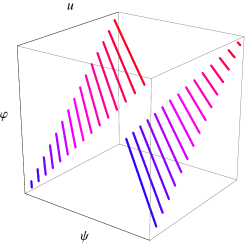
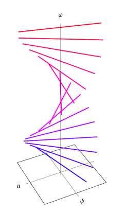
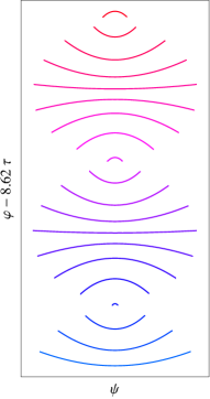
   Figure 1: The circular string (7), folded string (10), and LS’s solution (13). In all of these the lines from blue to red (and up the page) represent increasing time. The first has zero winding along $\varphi$ (i.e. $m_{\varphi}=0$) and $m_{\uppsi}=m_{u}=1$. In the last, we take $\nu=\tilde{\nu}=2$ and have subtracted off 90% of the motion along $\varphi$.

3. The final example is a folded spinning string, with the centre of mass moving in the $\varphi$ direction:

   $$\uppsi+i\,u=A\,e^{i\nu\tau}\cos\nu\sigma,\qquad\varphi=\upomega\tau,\qquad t=\kappa\tau.$$ (10)

   Here $\nu\in\mathbb{Z}$ counts the number of windings. When $A\to 0$ this becomes the supersymmetric BMN particle, and when $A\to\infty$ it stops moving along the equator. It has charges

   $$\Delta=4\pi g\>\kappa,\qquad J_{+}=J_{-}=J^{\prime}=4\pi g\>\upomega,\qquad S=2\pi g\>A^{2}\nu$$ (11)

   where $S$ is the angular momentum in the $\uppsi$-$u$ plane:

   $$S=R^{2}\int\frac{d\sigma}{2\pi}\operatorname{Im}\left[(\uppsi-i\,u)\>\partial_{\tau}(\uppsi+i\,u)\vphantom{1^{1^{1}}}\right].$$

   The contributions to the Virasoro constraints from particular spheres are quite complicated, for example:

   $$V_{S+}^{\text{diag}} =\cos^{2}\upphi\>\upomega^{2}+\sin\upphi\cos\upphi\>A\upomega\nu\>\cos\nu\sigma\>\sin\nu\tau+\sin^{2}\upphi\>\frac{A^{2}\nu^{2}}{2}\left(1-\cos 2\nu\sigma\>\sin 2\nu\tau\right)$$

   $$V_{u}^{\text{diag}} =\frac{A^{2}\nu^{2}}{2}\left(1+\cos 2\nu\sigma\>\sin 2\nu\tau\right)$$

   and off-diagonal

   $$V_{S+}^{\text{off}} =\sin\upphi\cos\upphi\>A\upomega\nu\>\sin\nu\sigma\>\cos\nu\tau+\sin^{2}\upphi\>\frac{A^{2}\nu^{2}}{4}\sin 2\nu\sigma\>\sin 2\nu\tau$$

   $$V_{u}^{\text{off}} =-\frac{A^{2}\nu^{2}}{4}\sin 2\nu\sigma\>\sin 2\nu\tau.$$

   However the total Virasoro constraints simply impose that the cusps are lightlike, $\kappa^{2}=\upomega^{2}+A^{2}\nu^{2}$, or in terms of the angular momenta,

   $$\kappa^{2}-\scalebox{0.95}{$\mathcal{J}$}^{2}=\frac{\nu}{2}\scalebox{0.95}{$\mathcal{S}$}$$ (12)

   where $\scalebox{0.95}{$\mathcal{S}$}=S/\sqrt{\lambda}$.

One of the solutions studied by [14] is related to this folded string. Both move in the $\varphi$ direction, but while our solution rotates in the $\uppsi$-$u$ plane, theirs is confined to $u=0$ and thus oscillates in $\varphi$. If we start from something very similar to (10)’s $\uppsi$ (agreeing exactly when $a=\tilde{a}=A/2$ and $\nu=\tilde{\nu}$):

$$\uppsi=a\,\cos\nu(\tau+\sigma)+\tilde{a}\,\cos\tilde{\nu}(\tau-\sigma)$$

and demand $u=0$, then we are led to

$$\varphi=\frac{\kappa}{2\nu}E\Big{(}\nu(\tau+\sigma)\Big{|}\frac{4a^{2}\nu^{2}}{\kappa^{2}}\Big{)}+\frac{\kappa}{2\tilde{\nu}}E\Big{(}\tilde{\nu}(\tau-\sigma)\Big{|}\frac{4\tilde{a}^{2}\tilde{\nu}^{2}}{\kappa^{2}}\Big{)}$$ (13)

very much like equation (4.48) of [14]. For this to be real we need $\kappa>2a\nu,2\tilde{a}\tilde{\nu}$, and for a closed string we need $a\nu=\tilde{a}\tilde{\nu}$. Plotting $\varphi$, it has some small fluctuations on top of rapid motion with $\tau$, as drawn in figure 1. Like our folded string, the contributions to the Virasoro constraint from each sphere are not constants. For example when $a=\tilde{a}=A/2$, $\nu=\tilde{\nu}=1$ and $\upphi=\tfrac{\pi}{4}$:

$$V_{S+}^{\text{diag}} =\frac{\kappa^{2}}{2}+\frac{A}{2}\sin(\sigma+\tau)\sqrt{\kappa^{2}-A^{2}\sin^{2}(\sigma+\tau)}-\frac{A}{2}\sin(\sigma-\tau)\sqrt{\kappa^{2}-A^{2}\sin^{2}(\sigma-\tau)}$$

$$V_{S+}^{\text{off}} =\frac{A}{4\sqrt{2}}\sin(\sigma+\tau)\sqrt{\kappa^{2}-A^{2}\sin^{2}(\sigma+\tau)}+\frac{A}{4\sqrt{2}}\sin(\sigma-\tau)\sqrt{\kappa^{2}-A^{2}\sin^{2}(\sigma-\tau)}$$

but clearly always $V_{u}=0$. Our solution (10), which explores also the $S^{1}$ direction, has the virtue of being much simpler, because it is rigidly rotating, and this allows us to calculate its mode frequencies below. We now turn to this problem.

2.2 Modes of the Circular String

The bosonic modes of (7) are easy to find, since this is a homogenous solution, i.e. $\partial_{\sigma}$ generates an isometry of target space. We make the following ansatz:

$$t =\kappa\tau+\tfrac{1}{\lambda^{1/4}}\tilde{t} \rho =0+\tfrac{1}{\lambda^{1/4}}\tilde{\rho}$$

$$\varphi_{+} =\upomega_{+}\tau+m_{+}\sigma+\tfrac{1}{\lambda^{1/4}}\cos\upphi\>\tilde{\varphi}_{+} \theta_{+} =\tfrac{\pi}{2}+\tfrac{1}{\lambda^{1/4}}\cos\upphi\>\tilde{\theta}_{+}$$ (14)

$$\varphi_{-} =\upomega_{-}\tau+m_{-}\sigma+\tfrac{1}{\lambda^{1/4}}\sin\upphi\>\tilde{\varphi}_{-} \theta_{-} =\tfrac{\pi}{2}+\tfrac{1}{\lambda^{1/4}}\sin\upphi\>\tilde{\theta}_{-}$$

$$u =\upomega_{u}\tau+m_{u}\sigma+\tfrac{1}{\lambda^{1/4}}\tilde{u}.$$

We set $\gamma=\beta_{\pm}=0$ on the understanding that $\tilde{\rho}$, $\tilde{\theta}_{+}$ and $\tilde{\theta}_{-}$ each represent one of two equivalent directions away from $\rho=0$ and $\theta_{\pm}=\frac{\pi}{2}$. We have also scaled $\tilde{\varphi}_{\pm},\tilde{\theta}_{\pm}$ so as to produce the canonical kinetic term in the quadratic Lagrangian:

$$2\mathcal{L}_{2B}=-\partial_{\mu}\tilde{t}\partial^{\mu}\tilde{t}+\sum_{x=\rho,\varphi_{\pm},\theta_{\pm},u}\partial_{\mu}\tilde{x}\partial^{\mu}\tilde{x}\;+\kappa^{2}\tilde{\rho}^{2}+(\upomega_{+}^{2}-m_{+}^{2})\tilde{\theta}_{+}^{2}+(\upomega_{-}^{2}-m_{-}^{2})\tilde{\theta}_{-}^{2}.$$

The solutions are all plane waves $\tilde{x}=C_{x}\exp(iw\tau+in\sigma)$ with $w=\sqrt{n^{2}+s^{2}}$, and we read off the following masses:

$$s^{2}=\begin{cases}\kappa^{2}&2\>AdS\mbox{ modes }(\tilde{\rho}\mbox{ etc.})\\ \upomega_{\pm}^{2}-m_{\pm}^{2}&4\,\perp\mbox{ sphere modes }(\tilde{\theta}_{\pm}\mbox{ etc.})\\ 0&4\>\mbox{massless }(\tilde{t},\tilde{\varphi}_{\pm},\tilde{u})\mbox{, of which 2 are gauge.}\end{cases}$$ (15)

Only the massless modes here influence the Virasoro constraints at leading order, and writing $E=i\,e^{iw_{n}\tau+in\sigma}/\lambda^{1/4}$ (with $w_{n}=\left|n\right|$) the changes are

$$\delta V_{AdS}^{\text{diag}} =-2C_{t}\,\kappa\,w_{n}\,E, \delta V_{AdS}^{\text{off}} =-C_{t}\,\kappa\,n\,E$$

$$\delta V_{S+}^{\text{diag}} =2C_{\varphi+}(\upomega_{+}w_{n}+m_{+}n)E/\cos\upphi, \delta V_{S+}^{\text{off}} =C_{\varphi+}(\upomega_{+}n+m_{+}w_{n})E/\cos\upphi$$ (16)

$$\delta V_{S-}^{\text{diag}} =2C_{\varphi-}(\upomega_{-}w_{n}+m_{-}n)E/\sin\upphi, \delta V_{S-}^{\text{off}} =C_{\varphi-}(\upomega_{-}n+m_{-}w_{m})E/\sin\upphi$$

$$\delta V_{u}^{\text{diag}} =2C_{u}(\upomega_{u}w_{n}+m_{u}n)E, \delta V_{u}^{\text{off}} =C_{u}(\upomega_{u}n+m_{u}w_{n})E.$$

To preserve the total Virasoro constraints (4) we can always solve for (say) $C_{t}$ and $C_{u}$, leaving $\tilde{\varphi}_{\pm}$ as physical modes. Doing so will not make individual contributions (such as $\smash{\delta V_{S+}^{\text{diag}}}$) constant, but let us observe that they will integrate to zero: $\smash{\int_{0}^{2\pi}d\sigma\>\delta V_{S+}^{\text{diag}}}=0$ etc.

The fermionic quadratic Lagrangian is given by

$$\hfill\mathcal{L}_{2F} =\left(\eta^{\mu\nu}\delta^{IJ}-\epsilon^{\mu\nu}\sigma_{3}^{IJ}\right)\mkern 1.0mu\overline{\mkern-1.0mu\Theta\mkern-1.5mu}\mkern 1.5mu^{I}\rho_{\mu}D_{\nu}\Theta^{J}$$

where $$\epsilon^{01}=1$$ and

$$\qquad D_{\mu}\Theta^{I} =\left(\partial_{\mu}+\tfrac{1}{4}\partial_{\mu}X^{M}\upomega_{M}^{AB}\Gamma_{AB}\right)\delta^{IJ}\Theta^{J}+F\rho_{\mu}\sigma_{1}^{IJ}\Theta^{J}$$

$$\rho_{\mu} =\partial_{\mu}X^{M}E_{M}^{A}\Gamma_{A}$$

$$F =\tfrac{1}{24}F_{ABC}^{(3)}\Gamma^{ABC}=\tfrac{6}{24}\left(\Gamma^{012}+\cos\upphi\,\Gamma^{345}+\sin\upphi\,\Gamma^{678}\right).$$

The equations of motion are [47, 48]

$$(\rho_{0}-\rho_{1})(D_{0}+D_{1})\Theta^{1}=0,\qquad(\rho_{0}+\rho_{1})(D_{0}-D_{1})\Theta^{2}=0.$$ (17)

For the circular string this is all quite simple, since the spin connection term is zero, and the projections of gamma-matrices have constant coefficients:

$$\rho_{0}=\kappa\Gamma_{0}+\frac{\upomega_{+}}{\cos\upphi}\Gamma_{4}+\frac{\upomega_{-}}{\sin\upphi}\Gamma_{7}+\upomega_{u}\Gamma_{9},\qquad\rho_{1}=\frac{m_{+}}{\cos\upphi}\Gamma_{4}+\frac{m_{-}}{\sin\upphi}\Gamma_{7}+m_{u}\Gamma_{9}\,.$$

Making the ansatz $\Theta^{I}=e^{i(w_{n}\tau+n\sigma)}\Theta_{0}^{I}$ and fixing $\kappa$-symmetry by defining $\Psi_{0}=(\rho_{0}-\rho_{1})\Theta_{0}^{1}$, we get

$$(w_{n}^{2}-n^{2})\Psi_{0}=(\rho_{0}-\rho_{1})F(\rho_{0}+\rho_{1})F\Psi_{0}\,.$$ (18)

The eigenvalues of the matrix on the right hand side give the following masses:

$$s^{2}=\frac{1}{4}\begin{cases}(\kappa-\upomega_{+}-\upomega_{-})^{2}-(m_{+}+m_{-})^{2}\\ (\kappa+\upomega_{+}-\upomega_{-})^{2}-(m_{+}-m_{-})^{2}\\ (\kappa-\upomega_{+}+\upomega_{-})^{2}-(m_{+}-m_{-})^{2}\\ (\kappa+\upomega_{+}+\upomega_{-})^{2}-(m_{+}+m_{-})^{2}.\end{cases}$$ (19)

Note that both bosonic and fermionic masses are independent of $\upphi$, and free of $\upomega_{u}$ and $m_{u}$. Thus the only effect of momentum $\upomega_{u}$ in the $S^{1}$ is through the Virasoro constraints, i.e. in allowing different choices for $\upomega_{\pm}$ compared to the $\upomega_{u}=0$ case.

2.3 Modes of the Point Particle

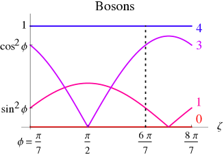
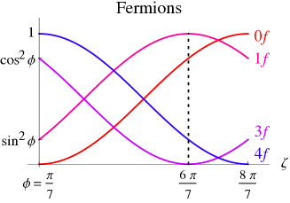
Figure 2: Masses $s/\kappa$ from (20) of modes of point particle solutions (5), for $\upphi=\pi/7$. The two extremes in the range of $\zeta$ drawn are BMN and a similar solution moving in the opposite direction, both of which are supersymmetric. The point of this is to illustrate that the fermions are re-organised by rotating $\zeta$ from one to the other. Notice that there is a third supersymmetric solution at $\zeta=\pi-\upphi$ (and similarly a fourth one at $\zeta=-\upphi$, not shown).

This solution (5) is just the special case $m_{\pm}=m_{u}=0$ and $\upomega_{u}=0$ of the circular string (7) treated above. Writing the masses (15) and (19) in terms of angles $\upphi$ and $\zeta$, and labelling them as in the algebraic curve, we have

$$s_{0} =0 s_{0f} =\tfrac{\kappa}{2}(1-\cos\upphi\cos\zeta-\sin\upphi\sin\zeta)$$

$$s_{1} =\kappa\left|\sin\upphi\sin\zeta\right| s_{1f} =\tfrac{\kappa}{2}(1-\cos\upphi\cos\zeta+\sin\upphi\sin\zeta)$$ (20)

$$s_{3} =\kappa\left|\cos\upphi\cos\zeta\right| s_{3f} =\tfrac{\kappa}{2}(1+\cos\upphi\cos\zeta-\sin\upphi\sin\zeta)$$

$$s_{4} =\kappa s_{4f} =\tfrac{\kappa}{2}(1+\cos\upphi\cos\zeta+\sin\upphi\sin\zeta).$$

The supersymmetric BMN case is $\zeta=\upphi$. Notice that as we rotate the direction in which the particle travels, the fermionic modes re-organise (see figure 2). Increasing $\zeta$ to $\upphi+\pi$, the heaviest fermion becomes massless (and vice versa), and we again have a supersymmetric solution. What we have done is to reverse the direction of motion of the string on the sphere: notice that the charges $J_{\pm}$ in (6) are both reversed.

While we will focus on the cases $\zeta=\upphi$ (BMN) and $\zeta=\upphi+\pi$ (reversed BMN), note that there are in all four supersymmetric points, as we recover the same list of masses at $\zeta=-\upphi$ and $\zeta=\pi-\upphi$. Physically these solutions reverse the direction of motion on just one $S^{3}$ (compared to BMN), visible in (6). In these cases the heavy and massless fermions of BMN become light modes (and vice versa).

2.4 Bosonic Modes of the Folded String

To treat the string (10) instead, it is simplest to work in Cartesian co-ordinates for the plane in which it rotates, i.e. to use $\uppsi$,$u$. Compared to the ansatz for the circular case (14) above, we need to replace $\varphi_{\pm},u$ with

$$\varphi =\upomega\tau+\tfrac{1}{\lambda^{1/4}}\tilde{\varphi}$$

$$\uppsi =A\,\cos\nu\tau\>\cos\nu\sigma+\tfrac{1}{\lambda^{1/4}}\tilde{\uppsi}$$

$$u =A\,\sin\nu\tau\>\cos\nu\sigma+\tfrac{1}{\lambda^{1/4}}\tilde{u}$$

and this leads to

$$2\mathcal{L}_{2B}=-\partial_{\mu}\tilde{t}\partial^{\mu}\tilde{t}+\sum_{x=\rho,\theta_{\pm},\varphi,\uppsi,u}\partial_{\mu}\tilde{x}\partial^{\mu}\tilde{x}\;+\kappa^{2}\tilde{\rho}^{2}+s_{\theta+}^{2}\tilde{\theta}_{+}^{2}+s_{\theta-}^{2}\tilde{\theta}_{-}^{2}.$$ (21)

As expected $\tilde{\uppsi},\tilde{u}$ remain massless, and the $AdS$ mode $\tilde{\rho}$ has mass $\kappa$. However the mass terms for the sphere modes $\tilde{\theta}_{\pm}$ are quite complicated. This is not unexpected, as the classical solution breaks translational invariance on the worldsheet. Written in terms of $\sigma^{\pm}=\tfrac{1}{2}(\sigma\pm\tau)$, we notice that they factorise:

$$s_{\theta+}^{2} =\Big{(}\upomega\,\cos^{2}\upphi+A\nu\,\sin\upphi\cos\upphi\,\sin 2\nu\sigma^{+}\Big{)}\Big{(}\upomega\,\cos^{2}\upphi-A\nu\,\sin\upphi\cos\upphi\,\sin 2\nu\sigma^{-}\Big{)}$$

$$s_{\theta-}^{2} =\Big{(}\upomega\,\sin^{2}\upphi-A\nu\,\sin\upphi\cos\upphi\,\sin 2\nu\sigma^{+}\Big{)}\Big{(}\upomega\,\sin^{2}\upphi+A\nu\,\sin\upphi\cos\upphi\,\sin 2\nu\sigma^{-}\Big{)}.$$

This points the way to solving the equations of motion $\partial_{+}\partial_{-}\tilde{\theta}=s_{\theta}^{2}\tilde{\theta}$ by using a separation of variables ansatz $\tilde{\theta}=P(\sigma^{+})M(\sigma^{-})$. We find the following solution, with $K$ the separation constant:

$$\tilde{\theta}_{+}(\sigma,\tau) =C\,e^{\frac{\upomega\,\cos^{2}\upphi}{2}\left(K+\frac{1}{K}\right)\sigma+\frac{\upomega\,\cos^{2}\upphi}{2}\left(K-\frac{1}{K}\right)\tau-A\frac{\sin\upphi\cos\upphi}{2}\left(K\cos 2\nu\sigma^{+}-\frac{1}{K}\cos 2\nu\sigma^{-}\right)}$$

$$=C\exp\left[in\sigma+iw_{n}\tau+\frac{iA\tan\upphi}{\upomega}\left(n\sin\nu\sigma\sin\nu\tau-w_{n}\cos\nu\sigma\cos\nu\tau\right)\right]$$ (22)

$$=C\exp\Big{(}i\,n\,\Sigma_{\frac{A}{\upomega}\tan\upphi}+i\,w_{n}\,T_{\frac{A}{\upomega}\tan\upphi}\Big{)},\qquad w_{n}=\sqrt{n^{2}+\upomega^{2}\cos^{4}\upphi}.$$

On the second line we solve $\frac{\upomega\,\cos^{2}\upphi}{2}\left(K+\frac{1}{K}\right)=i\,n$ with $n\in\mathbb{Z}$ to make it periodic in $\sigma$, and on the third we define

$$\Sigma_{A^{\prime}}=\sigma+A^{\prime}\>\sin\nu\sigma\sin\nu\tau,\qquad T_{A^{\prime}}=\tau-A^{\prime}\>\cos\nu\sigma\cos\nu\tau.$$ (23)

The modes on the other sphere are similar:

$$\tilde{\theta}_{-}(\sigma,\tau)=C\exp\Big{(}i\,n\,\Sigma_{-\frac{A}{\upomega}\cot\upphi}+i\,w_{n}\,T_{-\frac{A}{\upomega}\cot\upphi}\Big{)},\qquad w_{n}=\sqrt{n^{2}+\upomega^{2}\sin^{4}\upphi}.$$

We view the solution (22) as being a plane wave of mass $\upomega\cos^{2}\upphi$ in an unusual gauge (23). Performing the change of variables $(\sigma,\tau)\to(\Sigma_{A\tan\upphi/\upomega},T_{A\tan\upphi/\upomega})$ in the action produces the expected mass term:

$$\int d\tau\,d\sigma\left[\partial_{\mu}\tilde{\theta}_{+}\partial^{\mu}\tilde{\theta}_{+}+s_{\theta+}^{2}\tilde{\theta}_{+}^{2}\right]=\int dT\,d\Sigma\left[-\partial_{T}\tilde{\theta}_{+}\partial_{T}\tilde{\theta}_{+}+\partial_{\Sigma}\tilde{\theta}_{+}\partial_{\Sigma}\tilde{\theta}_{+}+\upomega^{2}\cos^{4}\upphi\>\tilde{\theta}_{+}^{2}\right]$$ (24)

since we have (writing $\Sigma^{M}$ for the new co-ordinates, $M=0,1$)

$$\det\left(\frac{\partial}{\partial\sigma^{\mu}}\Sigma_{\frac{A}{\upomega}\tan\upphi}^{M}\right)=\frac{s_{\theta+}^{2}}{\upomega^{2}\cos^{4}\upphi}.$$

In these new worldsheet co-ordinates the modes are orthogonal, which they are not in terms of the original $(\sigma,\tau)$:

$$\int_{0}^{2\pi}d\Sigma\operatorname{Re}\left[\tilde{\theta}_{+}(n)\right]\operatorname{Re}\left[\tilde{\theta}_{+}(n^{\prime})\right]\propto\delta_{n\,n^{\prime}}.$$

The appropriate Hamiltonian is then the one in terms of these variables, in which time translation is a symmetry of (24). Notice that there is a different $(\Sigma,T)$ for the modes in each $S^{3}$ (and different again for their superpartners, below).

Working out the effect of modes on the Virasoro constraint as in (16), again only the massless modes matter. The linear variations are

$$\delta V^{\text{diag}} =-2\kappa\>\partial_{\tau}\tilde{t}+2\upomega\>\partial_{\tau}\tilde{\varphi}+2A\nu\left(\cos\nu\sigma\cos\nu\tau\>\partial_{\tau}\tilde{u}-\sin\nu\sigma\sin\nu\tau\>\partial_{\sigma}\tilde{u}\right)$$

$$\qquad\qquad\qquad\qquad\quad-2A\nu\left(\cos\nu\sigma\sin\nu\tau\>\partial_{\tau}\tilde{\uppsi}+\sin\nu\sigma\cos\nu\tau\>\partial_{\sigma}\tilde{\uppsi}\right)$$ (25)

$$\delta V^{\text{off}} =-\kappa\>\partial_{\sigma}\tilde{t}+\upomega\>\partial_{\sigma}\tilde{\varphi}-A\nu\left(\sin\nu\sigma\sin\nu\tau\>\partial_{\tau}\tilde{u}-\cos\nu\sigma\cos\nu\tau\>\partial_{\sigma}\tilde{u}\right)$$

$$\qquad\qquad\qquad\qquad\;-A\nu\left(\sin\nu\sigma\cos\nu\tau\>\partial_{\tau}\tilde{\uppsi}+\cos\nu\sigma\sin\nu\tau\>\partial_{\sigma}\tilde{\uppsi}\right).$$

These constraints should (as always) kill two modes, leaving two physical massless modes. All must obey the massless wave equation $\partial_{+}\partial_{-}\tilde{x}=0$, but they cannot all be plane waves. There are nevertheless solutions which respect these constraints. For example if $\tilde{\uppsi}$ is a massless plane wave with $w_{n}=+n$, its effect can be cancelled by $\tilde{\varphi}$ as follows:

$$\tilde{\uppsi}=C_{\uppsi}e^{in(\sigma+\tau)},\qquad\tilde{\varphi}(\sigma^{+})=-\frac{C_{\uppsi}A\nu\>n}{\upomega(n^{2}-\nu^{2})}\>e^{in(\sigma+\tau)}\left(n\cos 2\nu\sigma^{+}-i\nu\sin 2\nu\sigma^{+}\right).$$ (26)

This $\tilde{\varphi}$ mode is a plane wave multiplied by another modulating factor, different to the one appearing in (22) but performing a similar role.

2.5 Fermionic Modes of the Folded String

The fermions can be analysed in a similar way. The spin connection term again vanishes, but the $\rho_{\mu}$ are more complicated than those for the circular string. Let us write them as follows:

$$\rho_{\pm}=\rho_{0}\pm\rho_{1} =\kappa\Gamma_{0}+R_{4\pm}(\sigma^{\pm})\>\Gamma_{4}+R_{7\pm}(\sigma^{\pm})\>\Gamma_{7}+R_{9}(\sigma^{\pm})\>\Gamma_{9}$$

with

$$R_{4\pm}(\sigma^{\pm}) =\upomega\cos\upphi\pm A\nu\sin\upphi\,\sin 2\nu\sigma^{\pm}$$

$$R_{7\pm}(\sigma^{\pm}) =\upomega\sin\upphi\mp A\nu\cos\upphi\,\sin 2\nu\sigma^{\pm}$$

$$R_{9}(\sigma^{\pm}) =A\nu\cos 2\nu\sigma^{\pm}$$

The equations of motion (17) can be written

$$\rho_{-}\partial_{+}\Theta^{1}+\rho_{-}F\rho_{+}\Theta^{2}=0,\qquad\rho_{+}\partial_{-}\Theta^{2}+\rho_{+}F\rho_{-}\Theta^{1}=0.$$

Now multiply from the left with $F$, and define some projected spinors

$$\Phi^{1}=F\rho_{-}\Theta^{1},\qquad\Phi^{2}=F\rho_{+}\Theta^{2}$$

and also the following functions:

$$G_{\pm}(\sigma^{\pm})=F\rho_{\pm}+\rho_{\pm}F=\tfrac{1}{2}\left(-\kappa\Gamma^{12}+\cos\upphi\>R_{4\pm}\>\Gamma^{35}+\sin\upphi\>R_{7\pm}\>\Gamma^{68}\right).$$

Then using that $F^{2}=0$ we obtain

$$\partial_{+}\Phi^{1}+G_{-}\Phi^{2}=0,\qquad\partial_{-}\Phi^{2}+G_{+}\Phi^{1}=0$$

and thus $\partial_{+}\partial_{-}\Phi^{I}+G_{+}G_{-}\Phi^{I}=0$. The matrices $G_{+}$ and $G_{-}$ commute, and we may expand the solution in their common eigenspinors $\epsilon_{r}$, which are constants:

$$G_{\pm}(\sigma^{\pm})\>\epsilon_{r}=g_{\pm r}(\sigma^{\pm})\>\epsilon_{r},\qquad\Phi^{I}(\sigma,\tau)=\sum_{r}\tilde{\upphi}_{r}^{I}(\sigma,\tau)\>\epsilon_{r}.$$

Then we obtain a factorised equation for the coefficient fields $\tilde{\upphi}_{r}^{I}$

$$\partial_{+}\partial_{-}\tilde{\upphi}_{r}^{I}=g_{+r}g_{-r}\tilde{\upphi}_{r}^{I}$$ (27)

in terms of the eigenvalues of $G_{\pm}$

$$g_{\pm r}(\sigma^{\pm})=\frac{i}{2}\Big{[}\alpha_{r}\kappa+\beta_{r}\cos\upphi\>R_{4\pm}(\sigma^{\pm})+\gamma_{r}\sin\upphi\>R_{7\pm}(\sigma^{\pm})\Big{]}$$

in which all eight choices of the signs $\alpha_{r},\beta_{r},\gamma_{r}=\pm 1$ occur.

We can solve (27) in the same way as we did the bosonic equation for $\tilde{\theta}_{\pm}$, and for the cases with signs $\beta_{r}\gamma_{r}=+1$ the result is simply a plane wave:

$$\tilde{\upphi}_{r}^{I}=C\,\exp\left(in\sigma+iw_{n}\tau\right),\qquad w_{n}=\sqrt{n^{2}+s_{r}^{2}},\qquad s_{r}=\frac{1}{2}\begin{cases}\kappa-\upomega,&r=0f\\ \kappa+\upomega,&r=4f\,.\end{cases}$$ (28)

The remaining cases are similar to (22):

$$\tilde{\upphi}_{r}^{I}=C\,\exp\left(in\tilde{\Sigma}_{\frac{A\sin 2\upphi}{2s_{r}}}+iw_{n}\tilde{T}_{\frac{A\sin 2\upphi}{2s_{r}}}\right),\qquad s_{r}=\frac{1}{2}\begin{cases}\kappa-\cos 2\upphi\>\upomega,&r=1f\\ \kappa+\cos 2\upphi\>\upomega,&r=3f\end{cases}$$ (29)

where $\tilde{\Sigma}_{A^{\prime}}=\sigma+A^{\prime}\cos\nu\sigma\cos\nu\tau$ and $\tilde{T}_{A^{\prime}}=\tau-A^{\prime}\sin\nu\sigma\sin\nu\tau$. The same comments made for the bosonic modes about the exotic gauge clearly also apply here.

When $A\to 0$ these modes all reduce to those of the BMN solution in (20). We have labelled them with names which make more sense in the algebraic curve formalism below.

3 Algebraic Curve

We begin by discussing the recent work of Lloyd and Stefański [14], who study (in section 4) a string moving in $\mathbb{R}\!\times\!S^{1}\!\times\!S^{1}$, with metric (3) at $\theta_{\pm}=\pi/2$, $\rho=0$ and $u=0$. The algebraic curve for this solution has three quasimomenta, and to avoid a clash of notation let us call their quasimomenta $\smash{\tilde{p}}_{l}$, with $l=0,1,2$ describing time, one sphere, and the other sphere. Their residues are parameterised by $\smash{\tilde{\kappa}}_{l}$ and $\smash{\tilde{m}}_{l}$:

$$\smash{\tilde{p}}_{l}(x)=\frac{\smash{\tilde{\kappa}}_{l}x+2\pi\smash{\tilde{m}}_{l}}{x^{2}-1}$$

which are given by

$$\smash{\tilde{\kappa}}_{0} =i\int_{0}^{2\pi}d\sigma\>\partial_{\tau}t, \smash{\tilde{\kappa}}_{1} =\frac{-1}{\cos\upphi}\int_{0}^{2\pi}d\sigma\>\partial_{\tau}\varphi_{+}, \smash{\tilde{\kappa}}_{2} =\frac{-1}{\sin\upphi}\int_{0}^{2\pi}d\sigma\>\partial_{\tau}\varphi_{-}$$ (30)

$$\smash{\tilde{m}}_{0} =0, 2\pi\smash{\tilde{m}}_{1} =\frac{-1}{\cos\upphi}\int_{0}^{2\pi}d\sigma\>\partial_{\sigma}\varphi_{+}, 2\pi\smash{\tilde{m}}_{2} =\frac{-1}{\sin\upphi}\int_{0}^{2\pi}d\sigma\>\partial_{\sigma}\varphi_{-}\,.$$

They showed that this is the complete algebraic curve for any solution in this spacetime, with only poles at $x=\pm 1$, never branch cuts.

The traditional Virasoro condition on the residues, applied to this case, reads

$$\sum_{l=0}^{D}(\smash{\tilde{\kappa}}_{l}\pm 2\pi\smash{\tilde{m}}_{l})^{2}=0,\qquad D=2.$$ (31)

The weaker generalised residue condition (GRC) proposed by [14] is that there exist $f_{l}^{\pm}(\sigma)$ such that

$$\smash{\tilde{\kappa}}_{l}\pm 2\pi\smash{\tilde{m}}_{l}=2\int_{0}^{2\pi}d\sigma\>f_{l}^{\pm}(\sigma),\qquad\sum_{l=0}^{D}(f_{l}^{\pm})^{2}=0.$$ (32)

Clearly if (31) is satisfied then we can simply take $f$ to be constant. Comments:

• The new condition is very close to being the worldsheet one. If we define

  $$f_{l}^{\pm}=G_{l}(\partial_{\tau}\varphi_{l}\pm\partial_{\sigma}\varphi_{l})$$

  writing $(G_{l},\varphi_{l})=(i,t),\;(\tfrac{1}{\cos\upphi},\varphi_{+}),\;(\tfrac{1}{\sin\upphi},\varphi_{-})$ for $l=0,1,2$, then the terms of the worldsheet Virasoro constraints (4) are

  $$V_{l}^{\text{diag}} =\frac{(f_{l}^{+})^{2}+(f_{l}^{-})^{2}}{2}=G_{l}^{2}(\partial_{\tau}\varphi_{l})^{2}+G_{l}^{2}(\partial_{\sigma}\varphi_{l})^{2}$$

  $$V_{l}^{\text{off}} =\frac{(f_{l}^{+})^{2}-(f_{l}^{-})^{2}}{4}=G_{l}^{2}\partial_{\tau}\varphi_{l}\>\partial_{\sigma}\varphi_{l}$$

  and thus (4), i.e. $\sum_{l}V_{l}^{\text{diag}}=0=\sum_{l}V_{l}^{\text{off}}$, is equivalent to (32). However this $f_{l}^{\pm}$ is a function of $\tau$ as well as $\sigma$.

• That the new condition (32) does not imply the traditional one (31) is a consequence of there being more than two factors in the spacetime. In fact without saying what $f$ means, the following implication is true for $D=1$

  $$0=\sum_{l=0}^{D}f_{l}^{2}(\sigma)\quad\Rightarrow\quad 0=\sum_{l=0}^{D}\left[\int d\sigma\>f_{l}(\sigma)\right]^{2}$$ (33)

  since $f_{0}=\pm if_{1}$, but fails for $D\geq 2$.

• Let us also mention here that if we consider a point particle solution in $\mathbb{R}\!\times\!(S^{1})^{D}$, then for $D=1$ there are just 2 solutions (lightlike and moving one way or the other) while in $D\geq 2$ there is a continuous set of them, allowing us to rotate from one direction to the reverse, as in figure 2.

3.1 Ten Dimensions

All string solutions in $\mathbb{R}\!\times\!S^{1}\!\times\!S^{1}$ will also be solutions in $AdS_{3}\!\times\!S^{3}\!\times\!S^{3}$, and thus we can map their algebraic curves into the one describing the full space. (Our notation here follows [42] closely.) This has six quasimomenta $p_{\ell}(x)$ with $\ell=1,2,3,\mkern 1.0mu\overline{\mkern-1.0mu1\mkern-1.5mu}\mkern 1.5mu,\mkern 1.0mu\overline{\mkern-1.0mu2\mkern-1.5mu}\mkern 1.5mu,\mkern 1.0mu\overline{\mkern-1.0mu3\mkern-1.5mu}\mkern 1.5mu$, corresponding to the six Cartan generators of $d(2,1;\alpha)$. The map is as follows:

$$\begin{pmatrix}p_{1}\\ p_{2}\\ p_{3}\end{pmatrix}=\begin{pmatrix}\frac{i}{2}\,\smash{\tilde{p}}_{0}-\frac{1}{2\sin\upphi}\,\smash{\tilde{p}}_{2}\\ i\,\smash{\tilde{p}}_{0}\\ \frac{i}{2}\,\smash{\tilde{p}}_{0}-\frac{1}{2\cos\upphi}\,\smash{\tilde{p}}_{1}\end{pmatrix},\qquad p_{\mkern 1.0mu\overline{\mkern-1.0mu\ell\mkern-1.5mu}\mkern 1.5mu}(\tfrac{1}{x})=p_{\ell}(x).$$ (34)

Inversion symmetry is $p_{\ell}(\tfrac{1}{x})=S_{\ell m}p_{m}(x)$ with $S=1_{3\!\times\!3}\otimes\big{[}\begin{smallmatrix}0&1\\ 1&0\end{smallmatrix}\big{]}$. The Cartan matrix is

$${A=\left[\begin{array}[]{ccc}4\sin^{2}\upphi&-2\sin^{2}\upphi&0\\ -2\sin^{2}\upphi&0&-2\cos^{2}\upphi\\ 0&-2\cos^{2}\upphi&4\cos^{2}\upphi\\[0.0pt] \@unrecurse}\end{array}\right]\otimes 1_{2\!\times\!2}.$$

for which we draw the Dynkin diagram , left and right. If we parameterise the poles at $\pm 1$ by $p_{\ell}(x)=(\kappa_{\ell}x+2\pi\,m_{\ell})/(x^{2}-1)$ as before, then the traditional condition on the residues is [12]

$$(\kappa_{\ell}\pm 2\pi m_{\ell})A_{\ell n}(\kappa_{n}\pm 2\pi m_{n})=0.$$ (35)

The angular momentum and winding (or worldsheet momentum) are given by the behaviour of the quasimomenta at infinity. In terms of $J_{\ell}$ defined as

$$p_{\ell}(x)\to P_{\ell}+\frac{1}{2gx}J_{\ell}+\mathcal{O}\Big{(}\frac{1}{x^{2}}\Big{)}.$$

the combinations of interest are

$$\Delta =\tfrac{1}{2}(-J_{2}+J_{\mkern 1.0mu\overline{\mkern-1.0mu2\mkern-1.5mu}\mkern 1.5mu}), J_{+} =(J_{3}-J_{\mkern 1.0mu\overline{\mkern-1.0mu3\mkern-1.5mu}\mkern 1.5mu})-\tfrac{1}{2}(J_{2}-J_{\mkern 1.0mu\overline{\mkern-1.0mu2\mkern-1.5mu}\mkern 1.5mu})$$

$$S =\tfrac{1}{2}(-J_{2}-J_{\mkern 1.0mu\overline{\mkern-1.0mu2\mkern-1.5mu}\mkern 1.5mu}), J_{-} =(J_{1}-J_{\mkern 1.0mu\overline{\mkern-1.0mu1\mkern-1.5mu}\mkern 1.5mu})-\tfrac{1}{2}(J_{2}-J_{\mkern 1.0mu\overline{\mkern-1.0mu2\mkern-1.5mu}\mkern 1.5mu})$$

and $J^{\prime}=\cos^{2}\upphi\>J_{+}+\sin^{2}\upphi\>J_{-}$. The combinations of $P_{\ell}$ of interest are discussed at (45) below.

In [42] another basis of quasimomenta $q_{i}(x)$, $i=1\ldots 6$ was defined, which are more closely related to the ones usually used in $AdS_{5}\!\times\!S^{5}$ or $AdS_{4}\!\times\!CP^{3}$, at least when $\upphi=\tfrac{\pi}{4}$. These are defined such that the Cartan matrix becomes trivial:

$${{\displaystyle\left(\begin{array}[]{c}q_{1}\\ \cr\kern-0.2pt\hrule height=0.4pt\kern-0.2pt}q_{3}\\ q_{5}\\[0.0pt] \end{array}\@unrecurse}\right) {{\displaystyle=B_{\text{left}}\begin{pmatrix}p_{1}\\ p_{2}\\ p_{3}\end{pmatrix},\qquad B_{\text{left}}=\left[\begin{array}[]{ccc}0&-1&0\\ \cr\kern-0.2pt\hrule height=0.4pt\kern-0.2pt}2\sin^{2}\upphi&-1&2\cos^{2}\upphi\\ -\sin 2\upphi&0&\sin 2\upphi\\[0.0pt] \end{array}\@unrecurse}\right]$$

$$\Rightarrow\quad q_{i}(\mathbb{I}_{1,2})_{ij}q^{\prime}_{j}=p_{\ell}A_{\ell m}p_{m}^{\prime}$$

writing $\mathbb{I}_{1,2}=\text{diag}(-1,1,1)$ to make the signature of weight space explicit. (After this we will simply write $q\cdot q^{\prime}$.) The right-hand quasimomenta $q_{i\,\text{even}}$ are given by the inversion symmetry $q_{i}(x)=-q_{i-1}(\tfrac{1}{x})$, and we may extend to $B=B_{\text{left}}\otimes\big{[}\begin{smallmatrix}1&0\\ 0&-1\end{smallmatrix}\big{]}$ to include them. Then $q_{1}$ and $q_{2}$ describe AdS, while $q_{3}\ldots q_{6}$ describe the spheres. It is also useful to think of $q_{-i}(x)=-q_{i}(x)$ as being 6 more quasimomenta, to distinguish the signs with which cuts connect them. (These are analogous to $q_{6}\ldots q_{10}$ in the $AdS_{4}\!\times\!CP^{3}$ case, at $\upphi=\tfrac{\pi}{4}$.)

Finally we will also need one more quasimomentum for the $S^{1}$ circle, which we can treat on the pattern of (30) above:

$$\smash{\tilde{p}}_{3}(x)=\frac{\smash{\tilde{\kappa}}_{3}x+2\pi\smash{\tilde{m}}_{3}}{x^{2}-1},\qquad\smash{\tilde{\kappa}}_{3}=-\int_{0}^{2\pi}d\sigma\>\partial_{\tau}u,\qquad 2\pi\smash{\tilde{m}}_{3}=-\int_{0}^{2\pi}d\sigma\>\partial_{\sigma}u\,.$$ (36)

We could then extend the sums in (31) and (32) to run up to $l=3$. For now however we make no attempt to include this as part of the $p_{\ell}$ (but see section 3.6 below).

3.2 The Generalised Vacuum

Zarembo [12] gives two solutions to $\vec{\kappa}\,A\,\vec{\kappa}\,=0$, $S\vec{\kappa}\,=-\vec{\kappa}\,$ for the case $\upphi=\frac{\pi}{4}$, i.e. to the Virasoro condition (in the absence of winding) and the inversion symmetry condition:

$$\vec{\kappa}\,=\left(0,1,0\right)\otimes(1,-1)\qquad\mbox{or }\quad\vec{\kappa}\,=\left(a,\>a^{2}+(1-a)^{2},\>1-a\right)\otimes(1,-1).$$

The first of these gives the BMN vacuum. However taking into account that the normalisation of this $\vec{\kappa}\,$ is arbitrary, the first is in fact the $a\to\infty$ case of the second, and thus the BMN vacuum is part of a one-parameter family. Choosing to use $\zeta$ as the parameter, restoring the $\upphi$ dependence, and fixing the overall normalisation, in this subsection we study the algebraic curve

$$p_{\ell}(x)=\frac{x}{x^{2}-1}\kappa_{\ell},\qquad\vec{\kappa}\,=-\frac{2\pi\kappa}{2}\left(1-\frac{\sin\zeta}{\sin\upphi},\;2,\;1-\frac{\cos\zeta}{\cos\upphi}\right)\otimes(1,-1)$$ (37)

corresponding to the point particle solution (5). It is also trivial to directly integrate (5) using (30) to find $\smash{\tilde{p}}_{l}$; the map (34) is fixed largely by this comparison. In the basis $q=Bp$ the same solution reads

$${{{{{{\left(\begin{array}[]{c}q_{1}(x)\\ \cr\kern-0.2pt\hrule height=0.4pt\kern-0.2pt}q_{3}(x)\\ q_{5}(x)\\[0.0pt] \end{array}\@unrecurse}\right)=\left(\begin{array}[]{c}-q_{2}(\tfrac{1}{x})\\ \cr\kern-0.2pt\hrule height=0.4pt\kern-0.2pt}-q_{4}(\tfrac{1}{x})\\ -q_{6}(\tfrac{1}{x})\\[0.0pt] \end{array}\@unrecurse}\right)=\frac{x}{x^{2}-1}\>2\pi\kappa\left(\begin{array}[]{c}1\\ \cr\kern-0.2pt\hrule height=0.4pt\kern-0.2pt}\cos(\upphi-\zeta)\\ \sin(\upphi-\zeta)\\[0.0pt] \end{array}\@unrecurse}\right)$$

which clearly solves $q\cdot q=0$ (in $\mathbb{R}^{2,4}$) and inversion symmetry. Again this reduces to the usual BMN solution when $\zeta=\upphi$.

We can now proceed to construct modes using the method of [26, 40]: we perturb the quasimomenta by adding new poles at $x=y$ and allowing the residues at $x=\pm 1$ to vary, subject to a condition on the behaviour at infinity. The perturbation of the energy is $\Omega(y)$, the “off-shell” frequency. The mode number $n\in\mathbb{Z}$ fixes the allowed points $y_{n}$, and thus gives the “on-shell” frequencies as $\upomega_{n}=\Omega(y_{n})$.

When we perturb the residues at $x=\pm 1$, we should do so in the most general way allowed by the Virasoro constraint. Since (37) is the most general solution (without winding) this means allowing

$$\delta\kappa_{\ell}=\frac{\partial\kappa_{\ell}}{\partial\kappa}\delta\kappa+\frac{\partial\kappa_{\ell}}{\partial\zeta}\delta\zeta\,.$$ (38)

The second term here is a new feature, arising because the Virasoro constraint has a one-parameter family of solutions (37), rather than the discrete solutions seen in $AdS_{5}\!\times\!S^{5}$ and $AdS_{4}\!\times\!CP^{3}$. Apart from this there are no changes to what was done in [42] for the $6+6$ modes considered there, and we recover most of the masses (20): bosons $r=1,3,4$, fermions $r=1f,3f,4f$, and their barred cousins. We refer to modes $1,1f,3,3f$ as light, since they have BMN masses $0<s<\kappa$, and modes $4,4f$ as heavy, BMN mass $\kappa$.

It will be instructive however to work one example out slowly, and we focus on the heavy fermion $4f$. This mode turns on nodes $1,2,3$, which we draw as and write as $k_{\ell}=-1$ for $\ell=1,2,3$. Thus we must consider

$$\delta p_{\ell}(x)=\delta\kappa_{\ell}\frac{x}{x^{2}-1}-\left[\frac{\alpha(y)}{x-y}+\frac{1}{2}\frac{\alpha(y)}{y}\right]\qquad\mbox{for}\;\ell=1,2,3$$

where $\alpha(y)=\frac{1}{2g}\frac{y^{2}}{y^{2}-1}$, and the other sheets are filled in by inversion symmetry $\delta p_{\mkern 1.0mu\overline{\mkern-1.0mu\ell\mkern-1.5mu}\mkern 1.5mu}(x)=\delta p_{\ell}(\tfrac{1}{x})$. We demand that at infinity,

$$\delta p_{\ell}(x) =\delta P_{\ell}+\frac{1}{2gx}\left(-1+D_{\ell}\delta\Delta\right)+\mathcal{O}\Big{(}\frac{1}{x^{2}}\Big{)},\qquad\ell=1,2,3$$

$$\delta p_{\mkern 1.0mu\overline{\mkern-1.0mu\ell\mkern-1.5mu}\mkern 1.5mu}(x) =\delta P_{\mkern 1.0mu\overline{\mkern-1.0mu\ell\mkern-1.5mu}\mkern 1.5mu}+\frac{1}{2gx}\>D_{\mkern 1.0mu\overline{\mkern-1.0mu\ell\mkern-1.5mu}\mkern 1.5mu}\delta\Delta+\ldots$$

where $D=B^{-1}(1,1\>|\,0,0,0,0)=\smash{\left(-\tfrac{1}{2},-1,-\tfrac{1}{2}\right)}\otimes(1,-1)$ encodes the change in energy. Solving, we find off-shell frequency

$$\Omega_{4f}(y)=\delta\Delta=\frac{\left[1+\cos(\upphi-\zeta)\right]}{y^{2}-1}$$ (39)

and momentum $\delta P_{\mkern 1.0mu\overline{\mkern-1.0mu1\mkern-1.5mu}\mkern 1.5mu}=\delta P_{\mkern 1.0mu\overline{\mkern-1.0mu3\mkern-1.5mu}\mkern 1.5mu}=n/4g\kappa$. To put this mode on shell we must solve for $y$ in terms of the mode number $n$ in

$$2\pi n_{4f} =-k_{\ell}A_{\ell m}p_{m}(y)=\left(A_{1m}+A_{2m}+A_{3m}\right)p_{m}(y)$$

$$=2\sin^{2}\upphi\>p_{1}-2\,p_{2}+2\cos^{2}\upphi\>p_{3}$$

$$=2\pi\kappa\left[1+\cos(\upphi-\zeta)\right]\frac{y}{y^{2}-1}$$ (40)

giving

$$y_{n}=\frac{\kappa}{2n}\left[1+\cos(\upphi-\zeta)\right]\pm\sqrt{1+\frac{\kappa^{2}}{4n^{2}}\left[1+\cos(\upphi-\zeta)\right]^{2}}.$$ (41)

The physical, on-shell frequency is then

$$\upomega_{n}=\Omega_{4f}(y_{n})=-\frac{1}{2}\left[1+\cos(\upphi-\zeta)\right]\pm\sqrt{\frac{n^{2}}{\kappa^{2}}+\frac{1}{4}\left[1+\cos(\upphi-\zeta)\right]^{2}}$$ (42)

and we choose always the positive sign here, which selects the pole in the physical region $\left|y_{n}\right|>1$. The mass $s_{4f}=\tfrac{\kappa}{2}\left[1+\cos(\upphi-\zeta)\right]$ matches the worldsheet calculation (20).

This mode is in fact a little simpler in terms of the basis $q$, where $4f=(1,-3)$, that is, it connects sheets $q_{1}$ and $q_{-3}=-q_{3}$. For the light modes we must set $\upphi=\pi/4$ to have this simple interpretation (away from this they influence more than two $q_{i}$) but for the heavy modes we do not need to do so. The equations above can be written

$${{{{{{\delta q(x)=\frac{2\pi\>x}{x^{2}-1}\left(\begin{array}[]{c}\delta\kappa\\ \delta\kappa\\ \cr\kern-0.2pt\hrule height=0.4pt\kern-0.2pt}c_{-}\,\delta\kappa+s_{-}\,\delta\zeta\\ c_{-}\,\delta\kappa+s_{-}\,\delta\zeta\\ s_{-}\,\delta\kappa-c_{-}\,\delta\zeta\\ s_{-}\,\delta\kappa-c_{-}\,\delta\zeta\\[0.0pt] \end{array}\@unrecurse}\right)+\left(\begin{array}[]{c}\left[\frac{\alpha(y)}{x-y}+\frac{1}{2}\frac{\alpha(y)}{y}\right]\\ 0\\ \cr\kern-0.2pt\hrule height=0.4pt\kern-0.2pt}-\left[\frac{\alpha(y)}{x-y}+\frac{1}{2}\frac{\alpha(y)}{y}\right]\\ 0\\ 0\\ 0\\[0.0pt] \end{array}\@unrecurse}\right)\to\frac{1}{2gx}\left(\begin{array}[]{c}\delta\Delta+1\\ \delta\Delta\\ \cr\kern-0.2pt\hrule height=0.4pt\kern-0.2pt}-1\\ 0\\ 0\\ 0\\[0.0pt] \end{array}\@unrecurse}\right)+\mathcal{O}\Big{(}\frac{1}{x^{2}}\Big{)}$$

(writing $c_{-}=\cos(\upphi-\zeta)$ and $s_{-}=\sin(\upphi-\zeta)$) and

$$2\pi n_{4f}=q_{1}(y)-q_{-3}(y)=q_{1}(y)+q_{3}(y)=2\pi\kappa\left[1+\cos(\upphi-\zeta)\right]\frac{y}{y^{2}-1}.$$

These give exactly the same results (41), (42).

3.3 Construction of Missing Fermions

Now recall our discussion of the modes of the point particle in the worldsheet theory, (20). We saw that moving from $\zeta=\upphi$ to $\zeta=\upphi+\pi$ (which reverses the direction of the BMN particle) made the heavy fermion $4f=(1,-3)$ become massless, and of course we recover this fact here, in (42). But we also saw that the massless fermion became heavy, and using this observation we can learn how to describe this mode (which we shall call “$0f$”) in the algebraic curve: it must be the mode which, near to $\zeta=\upphi+\pi$, behaves exactly like $4f$ did near to $\zeta=\upphi$.

In terms of the $q_{i}$ this is fairly obvious: increasing $\zeta\to\zeta+\pi$ changes $q_{3}\to-q_{3}$ and $q_{5}\to-q_{5}$, and thus we want $0f=(1,3)$. Translating back to the $p_{\ell}$ we find that $0f=\leavevmode\hbox to41.57pt{\vbox to7.43pt{\text{[drawing]}}}$, i.e. we turn on only the node $2$. We can then add this to the list of modes whose frequencies we can calculate by the procedure above. And it has exactly the mass expected from the worldsheet calculation.

Let us be a bit more careful: so far we have discussed the effect of reversing one particular solution (the vacuum) on one mode ($4f$). We would like to argue that the same idea holds more generally. Consider now some arbitrary algebraic curve $q(x)=B\,p(x)$, and define from this a reversed curve

$$q_{i}^{\prime}(x)=\begin{cases}q_{i}(x),&i=1,2\\ -q_{i}(x),&i=3,4,5,6\end{cases}\qquad\Leftrightarrow\quad p^{\prime}=B^{-1}q^{\prime}=\begin{pmatrix}-p_{1}+p_{2}\\ p_{2}\\ -p_{3}+p_{2}\end{pmatrix}.$$ (43)

This is also a valid solution. It has the same conserved charges in AdS but all of its sphere angular momenta are minus those of the initial solution. Then we ask: to reproduce the effect of a given mode $r$ on $q$, what mode $r^{\prime}$ must we use on $q^{\prime}$?

At $\upphi=\tfrac{\pi}{4}$ every mode $r=(i,j)$ connects two sheets $q_{i},q_{j}$. The mode number is

$$2\pi n=q_{i}-q_{j}\quad\to\quad 2\pi n^{\prime}=q^{\prime}_{i^{\prime}}-q^{\prime}_{j^{\prime}}.$$

For these to be equal, clearly we need $i^{\prime}=i$ for $i=1,2$ and $i^{\prime}=-i$ for $i\geq 3$. Then AdS bosons are unchanged, and for sphere bosons we need only change the sign of the mode number, $n^{\prime}=-n$, which we can ignore. But for fermions, which connect an AdS sheet to a sphere one, the change is $(i,j)\to(i^{\prime},j^{\prime})=(i,-j)$, i.e.

$$3f=(1,-5) \ \ \leftrightarrow\ \ 1f=(1,5) \mkern 1.0mu\overline{\mkern-1.0mu3\mkern-1.5mu}\mkern 1.5muf=(2,-6) \ \ \leftrightarrow\ \ \mkern 1.0mu\overline{\mkern-1.0mu1\mkern-1.5mu}\mkern 1.5muf=(2,6)$$ (44)

$$4f=(1,-3) \ \ \leftrightarrow\ \ 0f=(1,3) \mkern 1.0mu\overline{\mkern-1.0mu4\mkern-1.5mu}\mkern 1.5muf=(2,-4) \ \ \leftrightarrow\ \ \mkern 1.0mu\overline{\mkern-1.0mu0\mkern-1.5mu}\mkern 1.5muf=(2,4).$$

While we discussed the mode number, it is clear that the same thing happens for the placement of the new poles (cuts) into sheets: instead of connecting $i$ to $j$ we connect $i^{\prime}$ to $j^{\prime}$ by exactly the same rules. And while we have written this down in terms of the $q_{i}$, clearly (43) shows that the rule in terms of the $p_{\ell}$ is

$$\left(k{}_{1},k{}_{2},k{}_{3}\right)\to\left(k^{\prime}_{1},k^{\prime}_{2},k^{\prime}_{3}\right)=\left(-k_{1}+k_{2},\>k_{2},\>-k_{3}+k_{2}\right).$$

Applied to the list in table 1 we obtain the same map (44), now valid at any $\upphi$.

This map (44) takes the six original fermions (massive for BMN) and gives us a different set of six (massive for reversed BMN), with some overlap. We argue that the union of these two sets is precisely the full set of eight physical fermions which must always exist. For generic classical solutions they will all be nontrivial, and the simplest example of this is the non-supersymmetric point particle, (37). Perturbing this solution, the eight fermions $0f\ldots\mkern 1.0mu\overline{\mkern-1.0mu4\mkern-1.5mu}\mkern 1.5muf$ exactly reproduce the worldsheet masses (20). We will see similar agreement for other classical solutions below.

	$r$	BMN mass		Constraint on $\delta m_{\ell}$	At $\upphi=\tfrac{\pi}{4}$, $r=\hbox to0.0pt{$(i,j)$\hss}$
Massless:	$0$	0	—	—	—
	$0f$	0		$\delta P_{\mkern 1.0mu\overline{\mkern-1.0mu1\mkern-1.5mu}\mkern 1.5mu}=\delta P_{\mkern 1.0mu\overline{\mkern-1.0mu3\mkern-1.5mu}\mkern 1.5mu}=0$	$(1,3)$
Light:	$1$	$\kappa\sin^{2}\upphi$		$\delta P_{\mkern 1.0mu\overline{\mkern-1.0mu2\mkern-1.5mu}\mkern 1.5mu}=\delta P_{\mkern 1.0mu\overline{\mkern-1.0mu3\mkern-1.5mu}\mkern 1.5mu}=0$	$(3,5)$
	$1f$	$\kappa\sin^{2}\upphi$		$\delta P_{\mkern 1.0mu\overline{\mkern-1.0mu1\mkern-1.5mu}\mkern 1.5mu}=\delta P_{\mkern 1.0mu\overline{\mkern-1.0mu2\mkern-1.5mu}\mkern 1.5mu}$, $\delta P_{\mkern 1.0mu\overline{\mkern-1.0mu3\mkern-1.5mu}\mkern 1.5mu}=0$	$(1,5)$
	$3$	$\kappa\cos^{2}\upphi$		$\delta P_{\mkern 1.0mu\overline{\mkern-1.0mu1\mkern-1.5mu}\mkern 1.5mu}=\delta P_{\mkern 1.0mu\overline{\mkern-1.0mu2\mkern-1.5mu}\mkern 1.5mu}=0$	$(3,-5)$
	$3f$	$\kappa\cos^{2}\upphi$		$\delta P_{\mkern 1.0mu\overline{\mkern-1.0mu1\mkern-1.5mu}\mkern 1.5mu}=0$, $\delta P_{\mkern 1.0mu\overline{\mkern-1.0mu2\mkern-1.5mu}\mkern 1.5mu}=\delta P_{\mkern 1.0mu\overline{\mkern-1.0mu3\mkern-1.5mu}\mkern 1.5mu}$	$(1,-5)$
Heavy:	$4$	$\kappa$		$\delta P_{\mkern 1.0mu\overline{\mkern-1.0mu1\mkern-1.5mu}\mkern 1.5mu}=\tfrac{1}{2}\delta P_{\mkern 1.0mu\overline{\mkern-1.0mu2\mkern-1.5mu}\mkern 1.5mu}=\delta P_{\mkern 1.0mu\overline{\mkern-1.0mu3\mkern-1.5mu}\mkern 1.5mu}$	$(1,-1)$
	$4f$	$\kappa$		$\delta P_{\mkern 1.0mu\overline{\mkern-1.0mu1\mkern-1.5mu}\mkern 1.5mu}=\delta P_{\mkern 1.0mu\overline{\mkern-1.0mu2\mkern-1.5mu}\mkern 1.5mu}=\delta P_{\mkern 1.0mu\overline{\mkern-1.0mu3\mkern-1.5mu}\mkern 1.5mu}$	$(1,-3)$

Table 1: List of modes in the $AdS_{3}\!\times\!S^{3}\!\times\!S^{3}\!\times\!S^{1}$ algebraic curve, now including massless fermions. The colouring of the nodes is $-k_{\ell r}$ with $\leavevmode\hbox to7.23pt{\vbox to7.23pt{\text{[drawing]}}}=1$ and $\leavevmode\hbox to7.23pt{\vbox to7.23pt{\text{[drawing]}}}=2$. We omit here the right-hand modes $\mkern 1.0mu\overline{\mkern-1.0mu0\mkern-1.5mu}\mkern 1.5mu\ldots\mkern 1.0mu\overline{\mkern-1.0mu4\mkern-1.5mu}\mkern 1.5muf$, for which $k_{\ell\mkern 1.0mu\overline{\mkern-1.0mur\mkern-1.5mu}\mkern 1.5mu}=-k_{\ell r}$.

Some further comments:

• In the literature only the nodes $1$ and $3$ are described momentum-carrying, and thus it may seem a little puzzling that our $0f$ mode excites neither of them. However the notion of which nodes carry momentum depends on the choice of vacuum, and in general we should define

  $$P_{\zeta} =-\frac{1}{2\pi\kappa}\kappa_{\ell}A_{\ell m}P_{m}$$ (45)

  $$=-2\sin\upphi\sin\zeta\>(P_{1}-P_{\mkern 1.0mu\overline{\mkern-1.0mu1\mkern-1.5mu}\mkern 1.5mu})-\left[1-\cos(\upphi-\zeta)\right](P_{2}-P_{\mkern 1.0mu\overline{\mkern-1.0mu2\mkern-1.5mu}\mkern 1.5mu})-2\cos\upphi\cos\zeta\>(P_{3}-P_{\mkern 1.0mu\overline{\mkern-1.0mu3\mkern-1.5mu}\mkern 1.5mu}).$$

  At $\zeta=\upphi$ this gives the familiar

  $$P_{\upphi}=-2\sin^{2}\upphi\>(P_{1}-P_{\mkern 1.0mu\overline{\mkern-1.0mu1\mkern-1.5mu}\mkern 1.5mu})-2\cos^{2}\upphi\>(P_{3}-P_{\mkern 1.0mu\overline{\mkern-1.0mu3\mkern-1.5mu}\mkern 1.5mu}).$$

  At $\zeta=\upphi+\pi$, note that it is $4f$ which is does not appear to be momentum-carrying, while $0f$ carries $2$ units in the expected reversal of roles. When applied to the perturbations $\delta p$, this definition gives $\delta P=n/2g\kappa$ for all modes. If we interpret (42) as being a giant magnon dispersion relation, note that $4h^{2}\sin^{2}(\delta P/2)=n^{2}/\kappa^{2}$ as expected.

• One may wonder at this point whether there is a special connection between heavy and massless modes. (The heavy modes are, after all, composite objects in the same sense as in $AdS_{4}\!\times\!CP^{3}$.) We believe that this is not the case, because there are not just two supersymmetric pointlike solutions, but four: see figure 2. And going for instance from $\zeta=\upphi$ to $\zeta=\pi-\upphi$ re-organises $1f\leftrightarrow 4f$ and $3f\leftrightarrow 0f$ instead of (44), thus mixing light and massless modes instead (and also light and heavy). In place of (43) we should use

  $$p^{\prime\prime}(x)=\begin{pmatrix}p_{1}(x)\\ p_{2}(x)\\ -p_{3}(x)+p_{2}(x)\end{pmatrix}.$$

  This clearly gives the same re-organisation $1f\leftrightarrow 4f$ and $3f\leftrightarrow 0f$ for the modes of an arbitrary solution $p(x)$, not just the point particle. At $\upphi=\tfrac{\pi}{4}$ it reads $q_{1}^{\prime\prime}=q_{1}$, $q_{3}^{\prime\prime}=-q_{5}$ and $q_{5}^{\prime\prime}=-q_{3}$, but away from this it is more messy in terms of the $q_{i}$ (as we would expect).

• The list of allowed modes in table 1 is extra information not contained in the finite gap equations, usually written [1, 8]

  $$2\pi n_{\ell}=-A_{\ell j}\frac{\kappa_{j}x+2\pi m_{j}}{x^{2}-1}+A_{\ell m}\hbox to0.0pt{\;\,--\hss}\int dy\frac{\rho_{m}(y)}{x-y}-A_{\ell k}S_{km}\int\frac{dy}{y^{2}}\frac{\rho_{m}(y)}{x-\tfrac{1}{y}}.$$

  For example, the cut corresponding to the light boson “$3$” of course involves turning on density $\rho_{3}$ alone, with mode number $n=n_{3}$. But most of the other modes involve turning on several densities $\rho_{\ell}$ in a correlated way, and further allowing that only the sum of their $n_{\ell}$ will be an integer: for the light fermion $3f$ we have $n=n_{2}+n_{3}\in\mathbb{Z}$.

• In the worldsheet language we can embed $S_{+}^{3}\in\mathbb{C}^{2}$ by $X=(\sin\theta_{+}e^{i\varphi_{+}},\cos\theta_{+}e^{i\beta_{+}})$, and similarly $Y=(\sin\theta_{-}e^{i\varphi_{-}},\cos\theta_{-}e^{i\beta_{-}})$. The effect of (43) is then $X_{i}^{\prime}=X_{i}^{*}$ and $Y_{i}^{\prime}=Y_{i}^{*}$, or $\varphi_{\pm}^{\prime}=-\varphi_{\pm}$, $\beta_{\pm}^{\prime}=-\beta_{\pm}$, and this is clearly a symmetry of the action.

3.4 The Circular String

It is trivial to integrate the solution (7) using (30) and (36) to get the following residues:

$$\smash{\tilde{\kappa}}_{0} =i2\pi\kappa \smash{\tilde{\kappa}}_{1} =-2\pi\upomega_{+}/\cos\upphi \smash{\tilde{\kappa}}_{2} =-2\pi\upomega_{-}/\sin\upphi \smash{\tilde{\kappa}}_{3} =-2\pi\upomega_{u}$$ (46)

$$\smash{\tilde{m}}_{0} =im_{0}=0 \smash{\tilde{m}}_{1} =-m_{+}/\cos\upphi \smash{\tilde{m}}_{2} =-m_{-}/\sin\upphi \smash{\tilde{m}}_{3} =-m_{u}.$$

The traditional Virasoro condition (31) gives (setting $D=3$ there to include $\smash{\tilde{p}}_{3}$)

$$-(\kappa\pm m_{0})^{2}+\frac{(\upomega_{+}\pm m_{+})^{2}}{\cos^{2}\upphi}+\frac{(\upomega_{-}\pm m_{-})^{2}}{\sin^{2}\upphi}+(\upomega_{u}\pm m_{u})^{2}=0$$

agreeing with the worldsheet one (8). Again we write $m_{0}$ here just to allow for $\delta m_{0}$ in (48) below.

Mapping this into $AdS_{3}\!\times\!S^{3}\!\times\!S^{3}$ using (34), we ignore $\smash{\tilde{p}}_{3}$ (describing the $S^{1}$ factor) for now. The momentum carried is $P_{\mkern 1.0mu\overline{\mkern-1.0mu1\mkern-1.5mu}\mkern 1.5mu}=-m_{-}\pi/\sin^{2}\upphi$ and $P_{\mkern 1.0mu\overline{\mkern-1.0mu3\mkern-1.5mu}\mkern 1.5mu}=-m_{+}\pi/\cos^{2}\upphi$, which can be combined using (45) to give total momentum

$$P_{\zeta}=2\pi\left(m_{+}\frac{\cos\zeta}{\cos\upphi}+m_{-}\frac{\sin\zeta}{\sin\upphi}\right).$$

If we use the momentum assignments from the $\zeta=\upphi$ vacuum (or any supersymmetric vacuum) then $P_{\zeta}$ is a multiple of $2\pi$ (as expected for a closed string) whenever $m_{\pm}\in\mathbb{Z}$.

To construct modes for this solution, we need two extensions to what we have done above. First, we should allow the residues of the poles at $x=\pm 1$ to vary independently, but still subject to the Virasoro constraint. This means that we allow the windings $m_{\ell}$ to vary. Second, we find it necessary to demand that the resulting $\delta P_{\ell}$ belonging to nodes which are excited are all equal, and the others zero (and the same for the $\delta P_{\mkern 1.0mu\overline{\mkern-1.0mu\ell\mkern-1.5mu}\mkern 1.5mu}$ of the inverted sheets).

To be explicit, the perturbation of the quasimomenta is

$$\delta p_{\ell}(x)=k_{\ell}\left[\frac{\alpha(y)}{x-y}+\frac{1}{2}\frac{\alpha(y)}{y}\right]+S_{\ell m}k_{m}\left[\frac{\alpha(y)}{\frac{1}{x}-y}+\frac{1}{2}\frac{\alpha(y)}{y}\right]+\sum_{v}\frac{\partial p_{\ell}(x)}{\partial v}\delta v$$ (47)

where $v\in\{\kappa,\upomega_{\pm},m_{0},m_{\pm}\}$, subject to the following linearised Virasoro constraints:

$$\sum_{v}\frac{\partial V^{\text{diag}}}{\partial v}\delta v=0,\qquad\sum_{v}\frac{\partial V^{\text{off}}}{\partial v}\delta v=0.$$ (48)

We impose the following condition at infinity

$$\delta p_{\ell}(x)\to k_{\ell}\>\delta P_{\text{left}}-k_{\mkern 1.0mu\overline{\mkern-1.0mu\ell\mkern-1.5mu}\mkern 1.5mu}\>\delta P_{\text{right}}+\frac{1}{2gx}\left(k_{\ell}+D_{\ell}\delta\Delta\right)+\mathcal{O}\Big{(}\frac{1}{x^{2}}\Big{)}$$ (49)

and solve for $\delta v,\delta P_{\text{left}},\delta P_{\text{right}}$ and $\delta\Delta=\Omega_{r}(y)$. The on-shell frequency is found by solving

$$2\pi n=-k_{\ell}A_{\ell m}p_{m}(y_{n})$$

for $y_{n}$ and evaluating $\Omega(y_{n})$.

We can write all the results in a compact form, in terms of two numbers $S_{r}$ $M_{r}$:

$$\Omega_{r}(y)=\frac{1}{y^{2}-1}\frac{S_{r}^{2}-M_{r}^{2}}{\kappa S_{r}},\qquad 2\pi n_{r}=2\pi\frac{S_{r}y+M_{r}}{y^{2}-1}$$ (50)

for left-hand modes, and $2\pi n_{r}=2\pi\frac{S_{r}y+M_{r}y^{2}}{y^{2}-1}$ for right-hand (barred) modes. The on-shell frequency is then

$${\negthickspace\negthickspace\Omega_{r}(y_{n})=-\frac{S_{r}^{2}-M_{r}^{2}}{2\kappa S_{r}}-\left(n\pm\frac{M_{r}}{2}\right)\frac{M_{r}}{\kappa S_{r}}+\frac{1}{\kappa}\sqrt{\left(n\pm\frac{M_{r}}{2}\right)^{2}+\frac{S_{r}^{2}-M_{r}^{2}}{4}},\qquad\small r\in\negthickspace\begin{array}[]{l}\text{left}\\ \text{right.}\\[0.0pt] \@unrecurse}\end{array}$$ (51)

The coefficients here are the same left and right ($S_{r}=S_{\mkern 1.0mu\overline{\mkern-1.0mur\mkern-1.5mu}\mkern 1.5mu}$ and $M_{r}=M_{\mkern 1.0mu\overline{\mkern-1.0mur\mkern-1.5mu}\mkern 1.5mu}$) and are given by

$$S_{0} =2s_{0} M_{0} =0 S_{0f} =\kappa-\upomega_{+}-\upomega_{-} M_{0f} =-m_{+}-m_{-}$$ (52)

$$S_{1} =2\upomega_{-} M_{1} =2m_{-} S_{1f} =\kappa-\upomega_{+}+\upomega_{-} M_{1f} =-m_{+}+m_{-}$$

$$S_{3} =2\upomega_{+}\quad M_{3} =2m_{+}\qquad S_{3f} =\kappa+\upomega_{+}-\upomega_{-}\quad M_{3f} =m_{+}-m_{-}$$

$$S_{4} =2\kappa M_{4} =0 S_{4f} =\kappa+\upomega_{+}+\upomega_{-} M_{4f} =m_{+}+m_{-}.$$

The masses $s_{r}^{2}=(S_{r}^{2}-M_{r}^{2})/4$ are identical to those from the worldsheet calculation, (15) and (19). Some comments follow:

• Compared to the worldsheet results, the frequency (51) displays a shift in $n$ and a shift in energy. In the simplest case (9) $M_{r}/2\in\mathbb{Z}$ and thus the shift in $n$ will not matter, but in general it may be a half-integer, in which case according to [27] we should trust this not the worldsheet one. The term linear in $n$ vanishes in the sum. For the shifts in energy, note that we are still missing the massless bosons, and see discussion in [26, 41] .

• One surprising feature is that the “efficient” method [40] of constructing heavy modes off-shell by addition given by [42] fails here. The rules were

  $$1f+3f=4,\qquad 1+3f=1f+3=4f$$ (53)

  and these still hold at the level of $k_{\ell}$ of course (as is easily seen from table 1), but not at the level of $\Omega_{r}(y)$. We can observe however that (53) are not invariant under (44): the second equation becomes

  $$-1+1f=3f-3=0f.$$

• We discuss massless bosons in section 3.6 below.

3.5 The Folded String

Because the solution (10) also lives in $\mathbb{R}\!\times\!(S^{1})^{3}$ it is also described by only poles at $x=\pm 1$. We can use (30) and (36) to integrate and find their residues; notice that $A$ does not appear:

$$\smash{\tilde{\kappa}}_{0}=i2\pi\kappa,\qquad\smash{\tilde{\kappa}}_{1}=-2\pi\upomega\,\cos\upphi,\qquad\smash{\tilde{\kappa}}_{2}=-2\pi\upomega\,\sin\upphi,\qquad\smash{\tilde{\kappa}}_{3}=0.$$

Since (46) is the most general set of residues, we can describe this as a special case

$$\upomega_{+}=\upomega\>\cos^{2}\upphi,\qquad\upomega_{-}=\upomega\>\sin^{2}\upphi,\qquad m_{\pm}=0,\qquad\upomega_{u}=m_{u}=0.$$ (54)

An important difference from the circular string is that the traditional Virasoro constraint (31) is not obeyed. It gives $\kappa^{2}=\upomega^{2}$ here, contradicting the worldsheet one which gives $\kappa^{2}=A^{2}\nu^{2}+\upomega^{2}$, the physical condition that the cusps are lightlike. Thanks to [14] we understand that this is not a problem: (31) is too strict, and their GRC (32) allows for the residues seen here.

When we calculate modes of this solution, however, we demand that $\delta p(x)$ still obeys the linearised condition (48) derived from (8). Note that this was the only point at which the Virasoro constraints entered the mode computation for the circular string: at no point did we use the fact that the classical $p(x)$ obeys (8). And thus nothing changes in our calculation of the mode frequencies. Substituting (54) into the circular string’s mode masses, we obtain

$$s_{0f} =\tfrac{1}{2}(\kappa-\upomega)$$

$$s_{1} =\upomega\>\cos^{2}\upphi s_{1f} =\tfrac{1}{2}(\kappa+\upomega\,\cos 2\upphi)$$ (55)

$$s_{3} =\upomega\>\sin^{2}\upphi s_{3f} =\tfrac{1}{2}(\kappa-\upomega\,\cos 2\upphi)$$

$$s_{4} =\kappa s_{4f} =\tfrac{1}{2}(\kappa+\upomega).$$

These match what we got in the worldsheet theory, sections 2.4 and 2.5.

Using the linearised Virasoro condition (48) for these modes is justified by our worldsheet calculation. There we showed that, for both this solution and the circular string, only the massless bosons produce any change to any $\delta V_{l}$, the different factors’ contributions to the Virasoro constraint. Thus for all the modes studied here, the change to the integrated form (31) will be zero. (We believe this will be true for any classical solution.)

The classical solution (13) can be treated as a special case of the circular string in exactly the same way. Its residues $\smash{\tilde{\kappa}}_{l}$, $\smash{\tilde{m}}_{l}$ were written down in (4.49) of [14], and can be plugged into the masses $s_{r}^{2}=(S_{r}^{2}-M_{r}^{2})/4$ after using (46). Let us write just the special case $a=\tilde{a}$, $\nu=\tilde{\nu}$ which has zero winding, $\smash{\tilde{m}}_{l}=0$, and residues

$$\smash{\tilde{\kappa}}_{1}=-2\pi\upomega\,\cos\upphi,\qquad\smash{\tilde{\kappa}}_{2}=-2\pi\upomega\,\sin\upphi,\qquad\upomega=\frac{2\kappa}{\pi}\,E\Big{(}\frac{\pi}{2}\Big{|}\frac{4a^{2}\nu^{2}}{\kappa^{2}}\Big{)}.$$ (56)

Then its mode masses are given by (55) with this $\upomega$. Notice in particular that none of the fermionic modes of this are truly massless. In the limit $a\to 0$, in which this should approach the BMN solution, we have $E(\frac{\pi}{2}|m)=\frac{\pi}{2}-\frac{\pi}{8}m+\mathcal{O}(m^{2})$ and thus

$$\upomega=\kappa-\frac{a^{2}\nu^{2}}{\kappa}+\mathcal{O}(a^{4})\qquad\Rightarrow\qquad\begin{aligned} s_{0f}&=0+\frac{a^{2}\nu^{2}}{2\kappa}+\mathcal{O}(a^{4})\\ s_{1f}&=\kappa\>\cos^{2}\upphi-\frac{a^{2}\nu^{2}}{2\kappa}\cos 2\upphi+\mathcal{O}(a^{4}),\;\mbox{ etc.}\end{aligned}$$ (57)

While finding the modes of the exact macroscopic solution (13) in the worldsheet language seems hard, perhaps it would be possible to calculate these corrections to the BMN masses. This would be an interesting check of our methods.

3.6 Massless Bosons?

We showed above how to incorporate the massless fermions into the algebraic curve structure. Naturally we wonder if something similar can be done for the massless bosons, to capture all $8+8$ modes.

In the worldsheet language we know these modes exactly — they are fluctuations in directions in target space for which $\mathcal{L}_{2}$ is exactly the free Lagrangian $\partial_{\mu}\tilde{X}\,\partial^{\mu}\tilde{X}$ with no mass term, and the solutions are plane waves. These are precisely the directions within $\mathbb{R}\!\times\!(S^{1})^{3}$, for which we can use (30) to work out the algebraic curve. Since these equations are linear, we can also work out the change to the algebraic curve, regardless of the classical solution being perturbed. And the answer is simply zero. The pessimistic answer is thus that they are invisible to this formalism.

In table (52) we were a little more optimistic, and included $S_{0}=2s_{0}$ without having solved for it. We do this on the grounds that we believe (50) and (51) should, in the limit $s_{0}\to 0$, correctly describe this mode. To understand the limit we look at the $4f$ mode near to $s_{4f}=0$ (i.e. near to $\cos(\upphi-\zeta)=-1$). The energy (42) has the expected finite limit $\upomega_{n}=\left|n\right|/\kappa$, but this arises from dividing zero by zero: the off-shell frequency $\Omega(y)$ (39) appears to go to zero, but (holding $n$ fixed) the position of the pole $y_{n}$ from (40) also approaches $1$. The bosonic modes behave the same way, for instance the $3$ mode near to $\zeta=\pi/2$ (i.e. near to $J_{+}=0$).

Perhaps the same idea of everything converging on $x=1$ applies also to macroscopic classical solutions: moving in “massive” directions these would be described by one- or two-cut resolvents, but the “massless” versions studied here are described by just the poles.

Finally note that we have also largely ignored the $S^{1}$ direction $u$, which gives one of the massless bosons in the worldsheet picture. This appears to be correct in the sense that none of the worldsheet frequencies depend on the classical solution’s $\upomega_{u}$ and $m_{u}$. We constructed $\smash{\tilde{p}}_{3}$ in (36), and could write $p_{4}=-\smash{\tilde{p}}_{3}$ and $A_{\text{all}}=(A_{\text{left}}\oplus 1)\otimes 1_{2\!\times\!2}$. Then provided no modes turn on this node (i.e. $k_{4}=0$ always) nothing will change in our calculations.

4 Energy Corrections

The last two sections developed two ways to calculate mode frequencies of the “macroscopic massless” spinning strings that we are studying. The main reason to do so at all is to work out the one-loop correction to the energy, by adding these frequencies up.

For frequencies of the form $\upomega_{n}=\tfrac{1}{\kappa}\sqrt{(n+m)^{2}+s^{2}}$ (in which we allow some shift of the mode number by $m=\pm M_{r}/2$) the one-loop energy correction is

$$\delta E=\sum_{n=-N}^{N}e(n)=\sum_{r}(-1)^{F}\sum_{n=-N}^{N}\frac{1}{2\kappa}\sqrt{(n+m_{r})^{2}+s_{r}^{2}}$$ (58)

(defining $e(n)$ for use below). The simplest way to evaluate this sum is to approximate it with an integral: provided that $\sum_{r}(-1)^{F}=0$ and $\sum_{r}(-1)^{F}s_{r}^{2}=0$, to ensure (respectively) that the quadratic and logarithmic divergences cancel, we have

$$\delta E \approx\frac{\kappa}{2}\sum_{r}(-1)^{F}\int_{-N/\kappa}^{N/\kappa}dz\>\sqrt{\Big{(}z+\frac{m_{r}}{\kappa}\Big{)}^{2}+\Big{(}\frac{s_{r}}{\kappa}\Big{)}^{2}},\qquad z=n/\kappa$$

$$=\frac{1}{2\kappa}\sum_{r}(-1)^{F}\left[-s_{r}^{2}\log s_{r}+m_{r}^{2}\right].$$ (59)

Applying this method to the folded string, using the masses (55), it simplifies when we take the string to be short, $A^{2}\ll\kappa^{2}$. This is equivalent to taking $\upomega=\scalebox{0.95}{$\mathcal{J}$}$ large (compared to $\mathcal{S}$ ), and for the sake of familiarity we write all energy corrections in terms of these angular momenta. At $\upphi=\tfrac{\pi}{4}$ we get

$$\delta E =-\frac{\nu\scalebox{0.95}{$\mathcal{S}$}}{\mbox{$\scalebox{0.95}{$\mathcal{J}$}$}}\log 2+\frac{\nu^{2}\scalebox{0.95}{$\mathcal{S}$}^{2}}{8\scalebox{0.95}{$\mathcal{J}$}^{3}}\left[-3+6\log 2-4\log\scalebox{0.95}{$\mathcal{J}$}+\log\nu(\scalebox{0.95}{$\mathcal{S}$})\right]$$

$$\qquad+\frac{\nu^{3}\scalebox{0.95}{$\mathcal{S}$}^{3}}{8\scalebox{0.95}{$\mathcal{J}$}^{5}}\left[1-2\log 2+2\log\scalebox{0.95}{$\mathcal{J}$}-\log\nu(\scalebox{0.95}{$\mathcal{S}$})\right]+\mathcal{O}\Big{(}\frac{1}{\scalebox{0.95}{$\mathcal{J}$}^{5}}\Big{)}.$$

However this is almost certainly not what we want to do. For the case of $sl(2)$ circular strings in $AdS_{5}\!\times\!S^{5}$, agreement with the Bethe equations was seen by expanding $e(n)$ in large $\mathcal{J}$ first. Naively this leads to a divergent result, but Beisert and Tseytlin [24] showed how to re-sum the divergent terms. We now adapt what they did to the frequencies seen here, still focusing on the folded string.

4.1 Adapting the Beisert–Tseytlin procedure

The procedure given by [24] took $e(n)=\sum_{r}(-1)^{F_{r}}\upomega_{n}^{r}/2$ and divided it up as follows: After expanding in $\mathcal{J}\gg 1$ at fixed $n$ to get $\smash{e^{\text{sum}}}(n)$, they defined

$$\smash{e^{\text{sum}}_{\text{sing}}}(n) =\mbox{terms in }\smash{e^{\text{sum}}}(n)\mbox{ which give a divergence in the sum to }n=\infty,$$

$$\smash{e^{\text{sum}}_{\text{reg}}}(n) =\smash{e^{\text{sum}}}(n)-\smash{e^{\text{sum}}_{\text{sing}}}(n).$$

Then they wrote $n=\mathcal{J}x$ and expanded $e(\mathcal{J}x)$ in $\mathcal{J}\gg 1$ at fixed $x$ to get $\smash{e^{\text{int}}}(x)$, and similarly defined

$$\smash{e^{\text{int}}_{\text{sing}}}(x) =\mbox{terms in }\smash{e^{\text{int}}}(x)\mbox{ which give a divergence in the integral to }x=0,$$

$$\smash{e^{\text{int}}_{\text{reg}}}(x) =\smash{e^{\text{int}}}(x)-\smash{e^{\text{int}}_{\text{sing}}}(x).$$

It was observed that $\smash{e^{\text{sum}}_{\text{reg}}}(n)=\smash{e^{\text{int}}_{\text{sing}}}(n/\mathcal{J})$ and similarly $\smash{e^{\text{sum}}_{\text{sing}}}(n)=\smash{e^{\text{int}}_{\text{reg}}}(n/\scalebox{0.95}{$\mathcal{J}$}$), allowing them to exchange the singular part of a sum on $n$ for the regular part of an integral on $x$. The total energy correction was then

$$\delta E=\delta E^{\text{sum}}+\delta E^{\text{int}}=\sum_{n=-\infty}^{\infty}\smash{e^{\text{sum}}_{\text{reg}}}(n)+\int_{-\infty}^{\infty}\mathcal{J}dx\>\smash{e^{\text{int}}_{\text{reg}}}(x).$$ (60)

Here $\delta E^{\text{sum}}$ was the analytic part, containing only even powers of $\mathcal{J}=J/\sqrt{\lambda}$, and $\delta E^{\text{int}}$ was the non-analytic part, containing odd powers of $\mathcal{J}$. The necessity of reproducing such non-analytic terms is what led [24] to introduce the one-loop dressing phase in the Bethe equations.

Applying this procedure here, we find that $\smash{e^{\text{int}}_{\text{sing}}}(x)$ has odd powers including $1/x$ at $x=0$, which lead to terms in $\smash{e^{\text{int}}_{\text{reg}}}(x)$ which behave like $1/x$ at $x=\infty$, giving a logarithmically divergent answer. This problem does not arise in [24], nor in [28], where the divergent terms start only at order $1/x^{2}$ and at order $n^{2}$.

Let us consider the following modification of $e_{\text{sing}}$:

$$\smash{e^{\text{sum}}_{\text{sing}}}(n) =\left[\mbox{terms in }\smash{e^{\text{sum}}}(n)\mbox{ which go like }n^{0}\mbox{ or faster as }n\to\infty\right]$$

$$\qquad\qquad+\mu\left[\mbox{terms in }\smash{e^{\text{sum}}}(n)\mbox{ which go like }n^{-1}\mbox{ as }n\to\infty\right],$$ (61)

$$\smash{e^{\text{int}}_{\text{sing}}}(x) =\left[\mbox{terms in }\smash{e^{\text{int}}}(x)\mbox{ which go like }x^{-2}\mbox{ or faster as }x\to 0\right]$$

$$\qquad\qquad+\hat{\mu}\,\left[\mbox{terms in }\smash{e^{\text{int}}}(x)\mbox{ which go like }x^{-1}\mbox{ as }x\to 0\right].$$

Clearly $\mu=\hat{\mu}\,=1$ is the original procedure as described above, but the parameters $\mu,\hat{\mu}\,$ will let us control the new logarithmic divergences, without altering any results of [24, 28]. Introduce three explicit cutoffs as follows:

$$\delta E^{\text{sum}}=2\sum_{n=1}^{N}\smash{e^{\text{sum}}_{\text{reg}}}(n),\qquad\delta E^{\text{int}}=2\int_{\epsilon}^{\Lambda}\mathcal{J}dx\>\smash{e^{\text{int}}_{\text{reg}}}(x).$$ (62)

Treating the folded spinning string (using the masses (55), and writing $\scalebox{0.95}{$\mathcal{S}$}_{\nu}=\nu\,\scalebox{0.95}{$\mathcal{S}$}$) we obtain

$$\delta E^{\text{sum}} =\mbox{finite}+(\mu-1)\left(\log N+\gamma_{E}\vphantom{1^{1^{1}}}\right)\left[\frac{\scalebox{0.95}{$\mathcal{S}$}_{\nu}^{2}}{4\scalebox{0.95}{$\mathcal{J}$}^{3}}-\frac{\scalebox{0.95}{$\mathcal{S}$}_{\nu}^{3}}{2\scalebox{0.95}{$\mathcal{J}$}^{5}}+\frac{15\scalebox{0.95}{$\mathcal{S}$}_{\nu}^{4}}{16\scalebox{0.95}{$\mathcal{J}$}^{7}}+\mathcal{O}\Big{(}\frac{1}{\scalebox{0.95}{$\mathcal{J}$}^{9}}\Big{)}\right]$$

$$\delta E^{\text{int}} =\mbox{finite}+\left[\hat{\mu}\,\log\Lambda+(1-\hat{\mu}\,)\log\epsilon\vphantom{1^{1^{1}}}\right]\left[\frac{\scalebox{0.95}{$\mathcal{S}$}_{\nu}^{2}}{4\scalebox{0.95}{$\mathcal{J}$}^{3}}-\frac{\scalebox{0.95}{$\mathcal{S}$}_{\nu}^{3}}{2\scalebox{0.95}{$\mathcal{J}$}^{5}}+\frac{15\scalebox{0.95}{$\mathcal{S}$}_{\nu}^{4}}{16\scalebox{0.95}{$\mathcal{J}$}^{7}}+\ldots\right].$$ (63)

To match the upper cutoff of the sum with the lower cutoff of the integral, we want $N=\mathcal{J}\epsilon$. To cancel all three of the divergences, we need

$$N=e^{-\gamma_{E}}\>\Lambda^{\frac{\hat{\mu}\,}{1-\mu}}\>\epsilon^{\frac{1-\hat{\mu}\,}{1-\mu}}.$$

At $\mu=\hat{\mu}\,=\tfrac{1}{2}$, both of these conditions are solved by $N=\sqrt{\scalebox{0.95}{$\mathcal{J}$}}$, $\epsilon=1/\sqrt{\scalebox{0.95}{$\mathcal{J}$}}$, $\Lambda=e^{\gamma_{E}}\scalebox{0.95}{$\mathcal{J}$}$.

The other constraint on $\mu,\hat{\mu}\,$ is that we must again have $\smash{e^{\text{sum}}_{\text{reg}}}(n)=\smash{e^{\text{int}}_{\text{sing}}}(n/\mathcal{J})$, in order to omit $\smash{e^{\text{int}}_{\text{sing}}}$ and $\smash{e^{\text{sum}}_{\text{sing}}}$ from (60). The first few terms of these are

$$\smash{e^{\text{sum}}_{\text{reg}}}(n) =\frac{-\scalebox{0.95}{$\mathcal{S}$}_{\nu}^{2}\frac{(1-\mu)}{8n}}{\scalebox{0.95}{$\mathcal{J}$}^{3}}+\frac{\scalebox{0.95}{$\mathcal{S}$}_{\nu}^{3}\frac{(1-\mu)}{4n}+\scalebox{0.95}{$\mathcal{S}$}_{\nu}^{4}\frac{1}{128n^{3}}}{\scalebox{0.95}{$\mathcal{J}$}^{5}}-\frac{\scalebox{0.95}{$\mathcal{S}$}_{\nu}^{4}\frac{15(1-\mu)}{32n}+\scalebox{0.95}{$\mathcal{S}$}_{\nu}^{5}\frac{3}{128n^{3}}+\scalebox{0.95}{$\mathcal{S}$}_{\nu}^{6}\frac{1}{1024n^{5}}}{\scalebox{0.95}{$\mathcal{J}$}^{7}}+\mathcal{O}\Big{(}\frac{1}{\scalebox{0.95}{$\mathcal{J}$}^{7}}\Big{)}$$

$$\smash{e^{\text{int}}_{\text{sing}}}(n/\mathcal{J}) =\frac{-\scalebox{0.95}{$\mathcal{S}$}_{\nu}^{2}\frac{\hat{\mu}\,}{8n}}{\scalebox{0.95}{$\mathcal{J}$}^{3}}+\frac{\scalebox{0.95}{$\mathcal{S}$}_{\nu}^{3}\frac{\hat{\mu}\,}{4n}+\scalebox{0.95}{$\mathcal{S}$}_{\nu}^{4}\frac{1}{128n^{3}}}{\scalebox{0.95}{$\mathcal{J}$}^{5}}-\frac{\scalebox{0.95}{$\mathcal{S}$}_{\nu}^{4}\frac{15\hat{\mu}\,}{32n}+\scalebox{0.95}{$\mathcal{S}$}_{\nu}^{5}\frac{3}{128n^{3}}+\ldots}{\scalebox{0.95}{$\mathcal{J}$}^{7}}+\ldots$$ (64)

and clearly $\mu=\hat{\mu}\,=\tfrac{1}{2}$ gives agreement.

After cancelling these divergences, the finite parts are

$$\delta E^{\text{sum}} =\frac{\scalebox{0.95}{$\mathcal{S}$}_{\nu}^{4}\>\zeta(3)}{64\scalebox{0.95}{$\mathcal{J}$}^{5}}-\frac{\scalebox{0.95}{$\mathcal{S}$}_{\nu}^{5}\>24\zeta(3)+\scalebox{0.95}{$\mathcal{S}$}_{\nu}^{6}\>\zeta(5)}{512\scalebox{0.95}{$\mathcal{J}$}^{7}}$$

$$\qquad+\frac{\scalebox{0.95}{$\mathcal{S}$}_{\nu}^{6}\,\zeta(3)\,7\cdot 2^{-6}+\scalebox{0.95}{$\mathcal{S}$}_{\nu}^{7}\,\zeta(5)\,2^{-7}+\scalebox{0.95}{$\mathcal{S}$}_{\nu}^{8}\,\zeta(7)\,5\cdot 2^{-14}}{\scalebox{0.95}{$\mathcal{J}$}^{9}}+\mathcal{O}\Big{(}\frac{1}{\scalebox{0.95}{$\mathcal{J}$}^{11}}\Big{)}$$

and

$$\delta E^{\text{int}} =\frac{\mbox{$\scalebox{0.95}{$\mathcal{S}$}$}}{\mbox{$\scalebox{0.95}{$\mathcal{J}$}$}}\left[\alpha\log\alpha+(1-\alpha)\log(1-\alpha)\vphantom{1^{1^{1}}}\right]$$

$$\qquad+\frac{\scalebox{0.95}{$\mathcal{S}$}^{2}}{4\scalebox{0.95}{$\mathcal{J}$}^{3}}\left[(1-6\alpha)\log\alpha+(6\alpha-5)\log(1-\alpha)+\log 2-1\vphantom{1^{1^{1}}}\right]+\mathcal{O}\Big{(}\frac{1}{\scalebox{0.95}{$\mathcal{J}$}^{5}}\Big{)}.$$ (65)

Note that there appears to be no consistent pattern of even and odd powers, like that for the analytic / non-analytic distinction. Note also that only $\delta E^{\text{int}}$ depends on $\upphi$, which we write here as $\alpha=\cos^{2}\upphi$. At $\upphi=\pi/4$ our result is simpler,

$$\delta E^{\text{int}}=-\frac{\scalebox{0.95}{$\mathcal{S}$}_{\nu}\log 2}{\mbox{$\scalebox{0.95}{$\mathcal{J}$}$}}+\frac{\scalebox{0.95}{$\mathcal{S}$}_{\nu}^{2}(5\log 2-1)}{4\scalebox{0.95}{$\mathcal{J}$}^{3}}-\frac{\scalebox{0.95}{$\mathcal{S}$}_{\nu}^{3}(8\log 2-1)}{4\scalebox{0.95}{$\mathcal{J}$}^{5}}+\frac{\scalebox{0.95}{$\mathcal{S}$}_{\nu}^{4}(660\log 2-113)}{192\scalebox{0.95}{$\mathcal{J}$}^{7}}+\mathcal{O}\Big{(}\frac{1}{\scalebox{0.95}{$\mathcal{J}$}^{9}}\Big{)}.$$

Integrability normally gives an expansion in the Bethe coupling $h$, rather than $\sqrt{\lambda}$. These are related here by [51, 42, 28]

$$h(\lambda)=\frac{\sqrt{\lambda}}{2\pi}+c+\ldots=\frac{\sqrt{\lambda}}{2\pi}+\frac{\alpha\log\alpha+(1-\alpha)\log(1-\alpha)}{2\pi}+\mathcal{O}\Big{(}\frac{1}{\sqrt{\lambda}}\Big{)}.$$ (66)

If we regard the classical energy (12) as the zeroth term in an expansion in $h$, writing $\scalebox{0.95}{$\mathcal{J}$}_{\!\!h}=J/2\pi h$ (so that $\scalebox{0.95}{$\mathcal{J}$}_{\!\!h}=\scalebox{0.95}{$\mathcal{J}$}$ classically), then expanding in $\sqrt{\lambda}$ gives the following terms:

$$\Delta_{h=\infty} =2\pi h\sqrt{\scalebox{0.95}{$\mathcal{J}$}_{\!\!h}^{2}+2\nu\scalebox{0.95}{$\mathcal{S}$}_{h}}$$

$$=\sqrt{\lambda}\sqrt{\scalebox{0.95}{$\mathcal{J}$}^{2}+2\scalebox{0.95}{$\mathcal{S}$}_{\nu}}+\frac{2\pi c\,\scalebox{0.95}{$\mathcal{S}$}_{\nu}}{2\scalebox{0.95}{$\mathcal{J}$}\sqrt{\scalebox{0.95}{$\mathcal{J}$}^{2}+2\scalebox{0.95}{$\mathcal{S}$}_{\nu}}}+\mathcal{O}\Big{(}\frac{1}{\sqrt{\lambda}}\Big{)}$$

$$=\sqrt{\lambda}\sqrt{\scalebox{0.95}{$\mathcal{J}$}^{2}+2\scalebox{0.95}{$\mathcal{S}$}_{\nu}}+2\pi c\left[\frac{\scalebox{0.95}{$\mathcal{S}$}_{\nu}}{\mbox{$\scalebox{0.95}{$\mathcal{J}$}$}}-\frac{\scalebox{0.95}{$\mathcal{S}$}_{\nu}^{2}}{\scalebox{0.95}{$\mathcal{J}$}^{3}}+\frac{3\scalebox{0.95}{$\mathcal{S}$}_{\nu}^{3}}{2\scalebox{0.95}{$\mathcal{J}$}^{5}}+\mathcal{O}\Big{(}\frac{1}{\scalebox{0.95}{$\mathcal{J}$}^{7}}\Big{)}\right]+\mathcal{O}\Big{(}\frac{1}{\sqrt{\lambda}}\Big{)}.$$

The $\scalebox{0.95}{$\mathcal{S}$}/\scalebox{0.95}{$\mathcal{J}$}$ term here is exactly the first term seen in (65). But starting with the $1/\scalebox{0.95}{$\mathcal{J}$}^{3}$ term there are genuine $1/h$ corrections, i.e. $\mathcal{O}(h^{0})$ terms. The first few terms are

$$\delta\Delta_{h}=\frac{\scalebox{0.95}{$\mathcal{S}$}^{2}}{4\scalebox{0.95}{$\mathcal{J}$}^{3}}\left(L-1\right)-\frac{\scalebox{0.95}{$\mathcal{S}$}^{3}}{2\scalebox{0.95}{$\mathcal{J}$}^{5}}\left(L-\frac{5}{12}-\frac{1}{3\sin 2\upphi}\right)+\frac{15\scalebox{0.95}{$\mathcal{S}$}^{4}}{16\scalebox{0.95}{$\mathcal{J}$}^{7}}\left(L-\frac{5}{36}-\frac{2}{5\sin 2\upphi}-\frac{4}{45\sin^{2}2\upphi}\right)+\ldots$$

where $L=\log 2+(1-2\alpha)\log\alpha-(1-2\alpha)\log(1-\alpha)=\log 2+\cos 2\upphi\log(\tan^{2}\upphi$), and obviously $\sin 2\upphi=4\alpha(1-\alpha)$.

5 Conclusions

The results of this paper are as follows:

• We have introduced some classical string solutions which we think can be interpreted as macroscopic excitations of the massless modes of the BMN string. To describe one of these, the folded string, in the algebraic curve we must use [14]’s general residue condition, but the solution here presented is itself much simpler than their example requiring this. For this property it is necessary that contributions to Virasoro from different factors of the target space are not all constant.

• We have shown how to calculate the fermionic “$0f$” mode frequencies using the algebraic curve for the first time. This calculation uses only (a linearised form of) the traditional Virasoro constraint, and we discussed why this is so. For all the classical solutions considered here (except BMN) these modes are in fact no longer massless, and their masses agree with those from worldsheet computations. (By contrast the bosonic massless modes are always trivial.)

• We learned how to do this by studying the reversal symmetry $\upomega\to-\upomega$ which acts on fermion masses $s\to 1-s$. This has not been discussed in the literature, but it uses the vacuum solutions $\vec{\kappa}\,$ previously discarded as spurious, and here interpreted as non-BMN pointlike strings. We can see the same symmetry in $CP^{3}$ and $S^{5}$ cases, but it is not interesting in the absence of massless modes. Here it is part of a continuous transformation controlled by $\zeta$, which while not a symmetry, teaches us about the massless limit.

• We discovered that the folded string is a special case of circular string, as far as modes are concerned. We view this as the distinction between macroscopic one- and two-cut solutions disappearing as these cuts converge onto the poles at $x=\pm 1$, just as the microscopic cuts which describe the modes converge onto the poles as the mode becomes massless. The same agreement of frequencies is seen in the worldsheet language, up to the fact that the modes appear in a slightly strange gauge. (Perhaps this is a larger example of the frequency shifts seen for instance in [26, 27].)

• We calculated energy corrections $\delta E^{\text{sum}}$ and $\delta E^{\text{int}}$, which for massive spinning strings would be the analytic and non-analytic terms. The division between these two types of terms comes from a version of the Beisert–Tseytlin re-summing procedure, modified here to deal with logarithmic divergences. We see some $\cos^{2}\upphi$ dependence in $\delta E^{\text{int}}$ even when expanding in $h(\lambda)$.

There are many interesting open directions from here:

• Most obviously, the same reversal idea will allow us to describe in the algebraic curve the four fermions in $AdS_{3}\!\times\!S^{3}\!\times\!T^{4}$ which are massless for BMN (sometimes called the non-coset fermions). This is the topic of a forthcoming paper. Similar things can no doubt be done for $AdS_{2}\!\times\!S^{2}\!\times\!T^{6}$ [56, 57, 58], and for backgrounds with mixed RR and NS-NS flux, which are the topic of much recent interest [59, 60, 61, 62, 63, 64, 65, 66, 67].

• The list of modes in table 1 is slightly ad-hoc, constructed along the lines of earlier examples (such as table 2) so as to match the BMN spectrum [42], and now the $\zeta$-vacuum spectrum. Nevertheless it contains important extra information not present in the finite-gap equations, which follow directly from $A,S,\vec{\kappa}\,$. It should be possible to understand this more rigorously from representation theory.
  Such an understanding might also point out exactly how to deal with the massless bosons. Our approach here is to view the algebraic curve as just a tool for calculating mode frequencies, and in this view there is no need to think about them, since they always have $\upomega_{n}=\left|n\right|/\kappa$.

• The ultimate goal of studying these spinning strings is to make contact with the quantum integrable spin-chain picture. In the $T^{4}$ case this means the S-matrix of [15, 16] or rather the associated Bethe equations. This S-matrix contains dressing phases for the massless sector which are at present unknown.
  However the comparison can’t be exactly along the lines of what was done for $su(2)$ and $sl(2)$ spinning strings [24, 25], as there is no meaningful resolvent here. Our discussion of the massless limit of the modes indicates why: the cuts have collapsed into the poles at $x=\pm 1$.

• We observe that several quite different strings can have the same algebraic curve description: for example (54) and (56) can easily be made to co-incide exactly. Some related ideas were explored by [68], see also [69, 70].

• Finally we note that some issues to do with calculating the modes of folded strings (and other non-homogeneous classical solutions) were recently encountered by [71]. Our folded string is a simpler case, but their techniques may be necessary for more general solutions.

Acknowledgements

Chrysostomos Kalousios collaborated on related earlier work. We thank Romuald Janik, Antal Jevicki, Robert de Mello Koch, Olof Ohlsson Sax, Alessandro Sfondrini, Bogdan Stefański, Alessandro Torrielli and Konstantin Zarembo for helpful discussions.

Michael was supported by the UCT University Research Council, the Claude Leon Foundation, and an NRF Innovation Fellowship. Inês was partially supported by the FCT–Portugal fellowship SFRH/BPD/69696/2010 and by the NCN grant 2012/06/A/ST2/00396. We thank CERN for hospitality.

Appendix A Reversal Symmetry for $AdS_{4}\!\times\!CP^{3}$

Above we note that the symmetry which reverses the direction of motion on the sphere $\upomega\to-\upomega$ re-arranges the fermions $s\to 1-s$ . This appendix looks at the same idea in $AdS_{4}\!\times\!CP^{3}$, as a check on our understanding of the formalism.

We follow here the conventions of [12], in which the Cartan matrix is

$${A=\left[\begin{array}[]{ccccc}0&1\\ 1&-2&1\\ &1&0&-1&-1\\ &&-1&2\\ &&-1&&2\\[0.0pt] \@unrecurse}\end{array}\right]$$

and the generators in weight space $\Lambda_{\ell}\in\mathbb{R}^{2,3}$ are:

$${{{\begin{array}[]{cccccc|cr}\Lambda_{1}&\Lambda_{2}&\Lambda_{3}&\Lambda_{4}&\Lambda_{5}&\\ \hbox to0.0pt{ \leavevmode\hbox to102.37pt{\vbox to16.33pt{\text{[drawing]}}} \hss}&&&&&\\ 1&&&&&&B_{1}&i=3\\ \cr\kern-0.2pt\hrule height=0.4pt\kern-0.2pt}1&-1&&&\phantom{-1}&&F_{1}&1\\ &1&-1&&&&F_{2}&2\\ \cr\kern-0.2pt\hrule height=0.4pt\kern-0.2pt}&&-1&1&1&&B_{2}&4\\ \phantom{-1}&&&-1&1&&B_{3}&5\hbox to0.0pt{.\hss}\\[0.0pt] \end{array}\@unrecurse}$$

We think of this as the matrix $B_{i\ell}=(\Lambda_{\ell})_{i}$ such that $q_{i}=B_{i\ell}p_{\ell}$, where $p_{\ell}$ are the quasimomenta corresponding to Cartan generators $\Lambda_{\ell}$ i.e. to nodes of the Dynkin diagram, and $q_{i}$ are the quasimomenta with manifest $OSp(2,2|6)$ symmetry as in [72]. The lower five of these are defined $q_{11-i}=-q_{i}$, and $i=3,4,\ldots 8$ describe $CP^{3}$ while $i=1,2,9,10$ describe $AdS_{4}$. . Inversion symmetry $p(\tfrac{1}{x})=Sp(x)$ is simple in terms of the $q_{i}$:

$$q_{1}(x)=-q_{2}(\tfrac{1}{x}),\qquad q_{3}(x)=-q_{4}(\tfrac{1}{x}),\qquad q_{5}(x)=-q_{5}(\tfrac{1}{x}).$$

Zarembo [12] gives two vacua, the only solutions of $\vec{\kappa}\,A\,\vec{\kappa}\,=0$ and $S\,\vec{\kappa}\,=-\vec{\kappa}\,$, and discards the second of these:

$$p_{\ell}(x) =\frac{\Delta}{2g}\frac{x}{x^{2}-1}\kappa_{\ell},\quad\vec{\kappa}\,=(1,0,-1,0,0) \Rightarrow\,\quad q(x) =\frac{\Delta}{2g}\frac{x}{x^{2}-1}(1,1\>|\,1,1,0)$$ (67)

$$p_{\ell}^{\prime}(x) =\frac{\Delta}{2g}\frac{x}{x^{2}-1}\kappa^{\prime}_{\ell},\quad\vec{\kappa}\,^{\prime}=-(1,2,3,2,2) \Rightarrow\quad q^{\prime}(x) =\frac{\Delta}{2g}\frac{x}{x^{2}-1}(1,1\>|\,-1,-1,0).$$

Written in weight space, it is clear that the second one differs by a minus in the $CP^{3}$ sheets. It will thus differ by a minus in all its $SU(4)$ charges. But physically we expect this to be little different; there is nothing sacred about the direction of motion of the initial BMN particle.

The same symmetry will exist for an arbitrary solution: given some classical curve $q_{i}(x)$, the reversed curve

$$q_{i}^{\prime}(x)=\begin{cases}q_{i}(x),&i=1,2\mbox{ (and thus }9,10)\\ -q_{i}(x),&3\leq i\leq 8\end{cases}$$ (68)

is also a valid algebraic curve. This will have charges $J^{\prime}=-J$, $Q^{\prime}=-Q$ but should be physically equivalent. In particular the frequencies of its vibrational modes should be identical, but calculating these according to the usual rules [72] does not give the same answer. For instance, taking the example of the vacuum solution again, the heavy fermion $(1,7)$ has become massless, unlike any of the modes of the original solution:

$$2\pi n{}_{(1,7)} =q{}_{1}-q{}_{7}=2\frac{\Delta}{2g}\frac{x}{x^{2}-1}$$

$$2\pi n^{\prime}_{(1,7)} =q^{\prime}_{1}-q^{\prime}_{7}=0,\qquad 2\pi n^{\prime}{}_{(1,4)}=q^{\prime}_{1}+q^{\prime}_{7}=2\frac{\Delta}{2g}\frac{x}{x^{2}-1}.$$

What we should obviously do is to insert the same minus in the definition of the modes: if we include a $(1,4)$ mode for the primed quasimomenta (i.e. allow cuts connecting sheet $q^{\prime}_{1}$ not to $q^{\prime}_{7}=-q^{\prime}_{4}$ but to $+q^{\prime}_{4}$) then we will recover the same frequency as the $(1,7)$ mode on the unprimed quasimomenta.

Light Bosons:	$(4,5)$		$\circlearrowright-$
	$(4,6)$		$\circlearrowright-$
	$(3,5)$		$\circlearrowright-$
	$(3,6)$		$\circlearrowright-$
Light Fermions:	$(1,5)$		$\leftrightarrow$	$(1,6)$
	$(2,5)$		$\leftrightarrow$	$(2,6)$
Heavy Bosons, $CP$:	$(3,7)$		$\circlearrowright-$
$AdS$:	$(1,10)$		$\circlearrowright$
	$(1,9)$		$\circlearrowright$
	$(2,9)$		$\circlearrowright$
Heavy Fermions:	$(1,7)$		$\to$	$(1,4)$ *
	$(2,7)$		$\to$	$(2,4)$ *
	$(1,8)$		$\to$	$(3,1)$ *
	$(2,8)$		$\to$	$(3,2)$ *

Table 2: List of modes in the $AdS_{4}\!\times\!CP^{3}$ algebraic curve, with $\to$ indicating the effect of reversing the direction (68). A star marks modes which did not exist before. As before the colouring of the nodes is $-k_{\ell\,(i,j)}$ with $\leavevmode\hbox to7.23pt{\vbox to7.23pt{\text{[drawing]}}}=1$ and $\leavevmode\hbox to7.23pt{\vbox to7.23pt{\text{[drawing]}}}=2$, and $2\pi n=-k_{\ell\,(i,j)}A_{\ell m}p_{m}=q_{i}-q_{j}$.

We can do this for all the modes, and translating back to descriptions in terms of $p_{\ell}$ we get the map shown in table 2. The light modes just get re-arranged, and the heavy bosons are left alone. This map gives new modes only for the heavy fermions, marked with a star.

• Note that the list of allowed modes is extra information not encoded in the finite gap equations, by which in this case we mean (3.26) of [12]. Each mode is some correlated set of densities $\rho_{\ell}(y)$. This is true of both the original set of modes, from [72], and the new set for the reversed BMN solution.

• Notice that these new modes don’t excite either of the momentum-carrying nodes $\ell=4,5$, while all the old light modes excited one, and all the old heavy modes excited both. However our notion of which nodes are momentum-carrying depends on the choice of vacuum, and with the reversed BMN $\vec{\kappa}\,^{\prime}$ it is not only the nodes $\ell=4,5$:

  $$P =\kappa_{\ell}A_{\ell k}P_{k}=P_{4}+P_{5} \underset{\hskip 5.69054pt\hskip 56.9055pt1\hskip 12.80373pt\smash{\raisebox{8.53581pt}{\scriptsize{$1$}}}}{\raisebox{-2.84526pt}{ \leavevmode\hbox to75.72pt{\vbox to14.26pt{\text{[drawing]}}} }}$$

  $$P^{\prime} =\kappa^{\prime}_{\ell}A_{\ell k}P_{k}=-2P_{1}+2P_{3}-P_{4}-P_{5} \underset{\hskip 5.69054pt-2\hskip 12.80373pt\,\hskip 12.80373pt2\hskip 12.80373pt-1\hskip 12.80373pt\smash{\raisebox{8.53581pt}{\scriptsize{$-1$}}}}{\raisebox{-2.84526pt}{ \leavevmode\hbox to75.72pt{\vbox to14.26pt{\text{[drawing]}}} }}$$ (69)

  Counted according to $P^{\prime}$, the new heavy modes do all excite two momentum-carrying nodes.

• In the worldsheet string theory, $CP^{3}$ is described by $Z\in\mathbb{C}^{4}$ with $Z\sim\lambda Z$ for any $\lambda\in\mathbb{C}$. The effect of (68) here is to conjugate each embedding co-ordinate $Z_{i}^{\prime}=Z_{i}^{*}$, thus reversing all $CP^{3}$ angular momenta. This is clearly a symmetry of the action.

These features are the same as for the $AdS_{3}\!\times\!S^{3}\!\times\!S^{3}\!\times\!S^{1}$ case: there too the “$0f$” mode is obtained from the heavy fermion “$4f$”, and does not excite either of what were initially thought of as momentum-carrying nodes. The crucial difference is that in $AdS_{4}$ this is just some discrete symmetry, which we could avoid thinking about by always rotating our co-ordinates to put the particle’s momentum into a standard direction before working out the monodromy matrix. If someone else made a different choice there is no surprise that they end up using a slightly different formalism. In $AdS_{3}$ on the other hand, there is a continuous set of physically distinct (non-BPS) solutions connecting the two opposite directions, and the same formalism ought to cover all of them, or at least both ends. We only understood $6/8$ of this, at either end, but the connection enabled us to fill in the remaining $2/8$ of the whole.

In this regard $AdS_{5}\!\times\!S^{5}$ will be just like $AdS_{4}\!\times\!CP^{3}$: we can write down the modes for an alternative vacuum, the reversed BMN solution, but there is never a need to do so.

References

- [1] A. Babichenko, B. Stefański jr. and K. Zarembo, Integrability and the / correspondence, JHEP 03 (2010) 058 [arXiv:0912.1723].
- [2] S. Gukov, E. Martinec, G. W. Moore and A. Strominger, The search for a holographic dual to , Adv. Theor. Math. Phys. 9 (2005) 435–525 [arXiv:hep-th/0403090].
- [3] D. Tong, The holographic dual of , JHEP 04 (2014) 193 [arXiv:1402.5135].
- [4] A. Pakman, L. Rastelli and S. S. Razamat, A spin chain for the symmetric product , JHEP 05 (2010) 099 [arXiv:0912.0959].
- [5] O. Ohlsson Sax, A. Sfondrini and B. Stefanski, Integrability and the conformal field theory of the Higgs branch, arXiv:1411.3676.
- [6] P. Sundin and L. Wulff, Worldsheet scattering in /, JHEP 07 (2013) 007 [arXiv:1302.5349].
- [7] R. Roiban, P. Sundin, A. Tseytlin and L. Wulff, The one-loop worldsheet S-matrix for the superstring, JHEP 08 (2014) 160 [arXiv:1407.7883].
- [8] R. Borsato, O. Ohlsson Sax and A. Sfondrini, All-loop Bethe ansatz equations for /, JHEP 04 (2013) 116 [arXiv:1212.0505v3].
- [9] R. Borsato, O. Ohlsson Sax and A. Sfondrini, A dynamic S-matrix for /, JHEP 04 (2013) 113 [arXiv:1211.5119].
- [10] L. Bianchi, V. Forini and B. Hoare, Two-dimensional S-matrices from unitarity cuts, JHEP 07 (2013) 088 [arXiv:1304.1798].
- [11] L. Bianchi and B. Hoare, string S-matrices from unitarity cuts, JHEP 08 (2014) 097 [arXiv:1405.7947].
- [12] K. Zarembo, Algebraic curves for integrable string backgrounds, Proc. Steklov Inst. Math. 272 (2011) 275–287 [arXiv:1005.1342v2].
- [13] O. Ohlsson Sax, B. Stefański jr. and A. Torrielli, On the massless modes of the / integrable systems, JHEP 03 (2013) 109 [arXiv:1211.1952].
- [14] T. Lloyd and B. Stefański jr., / finite-gap equations and massless modes, JHEP 04 (2014) 179 [arXiv:1312.3268].
- [15] R. Borsato, O. Ohlsson Sax, A. Sfondrini and B. Stefański jr., All-loop worldsheet S-matrix for , Phys. Rev. Lett. 113 (2014) 131601 [arXiv:1403.4543].
- [16] R. Borsato, O. Ohlsson Sax, A. Sfondrini and B. Stefański jr., The complete worldsheet S-matrix, JHEP 10 (2014) 066 [arXiv:1406.0453].
- [17] V. A. Kazakov, A. Marshakov, J. A. Minahan and K. Zarembo, Classical / quantum integrability in AdS/CFT, JHEP 05 (2004) 024 [arXiv:hep-th/0402207].
- [18] V. A. Kazakov and K. Zarembo, Classical / quantum integrability in non-compact sector of AdS/CFT, JHEP 10 (2004) 060 [arXiv:hep-th/0410105].
- [19] S. Schäfer-Nameki, The algebraic curve of 1-loop planar SYM, Nucl. Phys. B714 (2005) 3–29 [arXiv:hep-th/0412254].
- [20] N. Beisert, V. A. Kazakov, K. Sakai and K. Zarembo, The algebraic curve of classical superstrings on , Commun. Math. Phys. 263 (2006) 659–710 [arXiv:hep-th/0502226].
- [21] S. Frolov and A. A. Tseytlin, Multi-spin string solutions in , Nucl. Phys. B668 (2003) 77–110 [arXiv:hep-th/0304255].
- [22] G. Arutyunov, J. G. Russo and A. A. Tseytlin, Spinning strings in : New integrable system relations, Phys. Rev. D69 (2004) 086009 [arXiv:hep-th/0311004].
- [23] I. Y. Park, A. Tirziu and A. A. Tseytlin, Spinning strings in : One-loop correction to energy in sector, JHEP 03 (2005) 013 [arXiv:hep-th/0501203].
- [24] N. Beisert and A. A. Tseytlin, On quantum corrections to spinning strings and Bethe equations, Phys. Lett. B629 (2005) 102–110 [arXiv:hep-th/0509084].
- [25] R. Hernández and E. López, Quantum corrections to the string Bethe ansatz, JHEP 07 (2006) 004 [arXiv:hep-th/0603204].
- [26] N. Gromov and P. Vieira, The superstring quantum spectrum from the algebraic curve, Nucl. Phys. B789 (2008) 175–208 [arXiv:hep-th/0703191].
- [27] V. Mikhaylov, On the fermionic frequencies of circular strings, J. Phys. A43 (2010) 335401 [arXiv:1002.1831].
- [28] M. Beccaria, F. Levkovich-Maslyuk, G. Macorini and A. Tseytlin, Quantum corrections to spinning superstrings in : determining the dressing phase, JHEP 04 (2013) 006 [arXiv:1211.6090].
- [29] H. de Vega and I. Egusquiza, Planetoid string solutions in (3+1) axisymmetric space-times, Phys. Rev. D54 (1996) 7513–7519 [arXiv:hep-th/9607056].
- [30] S. S. Gubser, I. R. Klebanov and A. M. Polyakov, A semi-classical limit of the gauge/string correspondence, Nucl. Phys. B636 (2002) 99–114 [arXiv:hep-th/0204051].
- [31] S. Frolov and A. A. Tseytlin, Semiclassical quantization of rotating superstring in , JHEP 06 (2002) 007 [arXiv:hep-th/0204226v5].
- [32] T. McLoughlin, R. Roiban and A. A. Tseytlin, Quantum spinning strings in : testing the Bethe ansatz proposal, JHEP 11 (2008) 069 [arXiv:0809.4038].
- [33] N. Gromov and S. Valatka, Deeper look into short strings, JHEP 03 (2012) 058 [arXiv:1109.6305].
- [34] C. Lopez-Arcos and H. Nastase, Eliminating ambiguities for quantum corrections to strings moving in , Int. J. Mod. Phys. A28 (2013) 1350058 [arXiv:1203.4777].
- [35] V. Forini, V. Giangreco M. Puletti and O. Ohlsson Sax, Generalized cusp in and more one-loop results from semiclassical strings, J. Phys. A46 (2012) 115402 [arXiv:1204.3302v3].
- [36] L. Bianchi, M. S. Bianchi, A. Bres, V. Forini and E. Vescovi, Two-loop cusp anomaly in ABJM at strong coupling, JHEP 10 (2014) 013 [arXiv:1407.4788].
- [37] A. A. Tseytlin, Review of AdS/CFT integrability, chapter ii.1: Classical string solutions, Lett. Math. Phys. 99 (2012) 103–125 [arXiv:1012.3986].
- [38] T. McLoughlin, Review of AdS/CFT integrability, chapter ii.2: Quantum strings in , Lett. Math. Phys. 99 (2012) 127–148 [arXiv:1012.3987].
- [39] S. Schäfer-Nameki, Exact expressions for quantum corrections to spinning strings, Phys. Lett. B639 (2006) 571–578 [arXiv:hep-th/0602214].
- [40] N. Gromov, S. Schäfer-Nameki and P. Vieira, Efficient precision quantization in AdS/CFT, JHEP 12 (2008) 013 [arXiv:0807.4752].
- [41] M. C. Abbott, I. Aniceto and D. Bombardelli, Quantum strings and the / interpolating function, JHEP 12 (2010) 040 [arXiv:1006.2174].
- [42] M. C. Abbott, Comment on strings in at one loop, JHEP 02 (2013) 102 [arXiv:1211.5587].
- [43] M. C. Abbott, The Hernández–López phases: a semiclassical derivation, J. Phys. A46 (2013) 445401 [arXiv:1306.5106].
- [44] D. M. Hofman and J. M. Maldacena, Giant magnons, J. Phys. A39 (2006) 13095–13118 [arXiv:hep-th/0604135].
- [45] F. Lund and T. Regge, Unified approach to strings and vortices with soliton solutions, Phys. Rev. D14 (1976) 1524.
- [46] D. E. Berenstein, J. M. Maldacena and H. S. Nastase, Strings in flat space and PP waves from super Yang Mills, JHEP 04 (2002) 013 [arXiv:hep-th/0202021].
- [47] J. A. Minahan, Zero modes for the giant magnon, JHEP 02 (2007) 048 [arXiv:hep-th/0701005].
- [48] M. C. Abbott and I. V. Aniceto, Vibrating giant spikes and the large-winding sector, JHEP 06 (2008) 088 [arXiv:0803.4222].
- [49] N. Beisert and L. Freyhult, Fluctuations and energy shifts in the Bethe ansatz, Phys. Lett. B622 (2005) 343–348 [arXiv:hep-th/0506243].
- [50] N. Gromov, S. Schäfer-Nameki and P. Vieira, Quantum wrapped giant magnon, Phys. Rev. D78 (2008) 026006 [arXiv:0801.3671].
- [51] P. Sundin and L. Wulff, Classical integrability and quantum aspects of the superstring, JHEP 10 (2012) 109 [arXiv:1207.5531].
- [52] N. Gromov and V. Mikhaylov, Comment on the scaling function in , JHEP 04 (2009) 083 [arXiv:0807.4897].
- [53] D. Astolfi, V. Giangreco M Puletti, G. Grignani, T. Harmark and M. Orselli, Finite-size corrections for quantum strings on , JHEP 05 (2011) 128 [arXiv:1101.0004].
- [54] M. C. Abbott and P. Sundin, The near-flat-space and BMN limits for strings in at one loop, J. Phys. A45 (2012) 025401 [arXiv:1106.0737].
- [55] N. Gromov and G. Sizov, Exact slope and interpolating functions in ABJM theory, Phys. Rev. Lett. 113 (2014) 121601 [arXiv:1403.1894].
- [56] D. Sorokin, A. Tseytlin, L. Wulff and K. Zarembo, Superstrings in , J. Phys. A44 (2011) 275401 [arXiv:1104.1793].
- [57] M. C. Abbott, J. Murugan, P. Sundin and L. Wulff, Scattering in / and the BES phase, JHEP 10 (2013) 066 [arXiv:1308.1370].
- [58] B. Hoare, A. Pittelli and A. Torrielli, S-matrix for the massive and massless modes of the superstring, JHEP 11 (2014) 051 [arXiv:1407.0303].
- [59] B. Hoare and A. Tseytlin, On string theory on with mixed 3-form flux: tree-level S-matrix, Nucl. Phys. B873 (2013) 682–727 [arXiv:1303.1037].
- [60] B. Hoare, A. Stepanchuk and A. Tseytlin, Giant magnon solution and dispersion relation in string theory in with mixed flux, Nucl. Phys. B879 (2013) 318–347 [arXiv:1311.1794].
- [61] L. Wulff, Superisometries and integrability of superstrings, JHEP 05 (2014) 115 [arXiv:1402.3122].
- [62] J. R. David and A. Sadhukhan, Spinning strings and minimal surfaces in with mixed 3-form fluxes, JHEP 19 (2014) 049 [arXiv:1405.2687].
- [63] A. Babichenko, A. Dekel and O. Ohlsson Sax, Finite-gap equations for strings on with mixed 3-form flux, JHEP 11 (2014) 122 [arXiv:1405.6087].
- [64] R. Hernández and J. M. Nieto, Spinning strings in with NS-NS flux, Nucl. Phys. B888 (2014) 236–247 [arXiv:1407.7475].
- [65] T. Lloyd, O. Ohlsson Sax, A. Sfondrini and B. Stefański jr., The complete worldsheet S-matrix of superstrings on with mixed three-form flux, arXiv:1410.0866.
- [66] P. Sundin and L. Wulff, One- and two-loop checks for the superstring with mixed flux, arXiv:1411.4662.
- [67] A. Stepanchuk, String theory in with mixed flux: semiclassical and 1-loop phase in the S-matrix, arXiv:1412.4764.
- [68] R. A. Janik and P. Laskoś-Grabowski, Surprises in the AdS algebraic curve constructions – Wilson loops and correlation functions, Nucl. Phys. B861 (2012) 361–386 [arXiv:1203.4246].
- [69] S. Ryang, Algebraic curves for long folded and circular winding strings in , JHEP 02 (2013) 107 [arXiv:1212.6109].
- [70] A. Dekel, Algebraic curves for factorized string solutions, JHEP 04 (2013) 119 [arXiv:1302.0555].
- [71] V. Forini, V. Giangreco M Puletti, M. Pawellek and E. Vescovi, One-loop spectroscopy of semiclassically quantized strings: bosonic sector, J. Phys. A48 (2015) 085401 [arXiv:1409.8674].
- [72] N. Gromov and P. Vieira, The / algebraic curve, JHEP 02 (2008) 040 [arXiv:0807.0437].