Stochastic Navier-Stokes Equations in Unbounded Channel Domains

Abstract.

In this paper we prove the existence and uniqueness of path-wise strong solution to stochastic viscous flow in unbounded channels with multiple outlets using local monotonicity arguments. We devise a construction for solvability using a stochastic basic vector field.

1. Introduction

This paper concerns with stochastic fluid dynamics in unbounded channel domains with noncompact boundaries generalizing the deterministic results in Sritharan [62]. Mathematical theory of viscous incompressible flow through unbounded channel has many applications such as hydraulics in water resources, hydraulic machinery, oil transport networks, flow in engines etc. Well-posedness theorem is an essential step for applications in optimal control theory (Sritharan [64]), convergence of numerical algorithms and nonlinear filtering (Sritharan [63], Fernando and Sritharan [23]). Solvability theory of generalized solutions to Navier-Stokes equations was pioneered by Leray [41], Hopf [31] and Ladyzhenskaya [35], [36]. Steady state flow through channels of various kinds has been studied by a number of authors including Amick [4], [5], Amick and Franenkel [6], Ladyzhenskaya and Solonnikov [37], [38], [39]. In [4], Amick discussed the steady flow of viscous incompressible fluid in channels and pipes in two and three dimensions which are cylindrical outside some compact set. The paper by Heywood [28] highlighted the question of uniqueness of the solution of the Navier-Stokes equations for certain unbounded domains modeling channels, tubes, or conduits of some kind and the importance of prescribing flux or the overall pressure difference. In [6], Amick and Fraenkel studied steady state solutions of the Navier-Stokes equations in various types of two dimensional channel domains. In [29], Heywood constructed classical solutions of the Navier-Stokes equations for both stationary and non-stationary boundary value problems in arbitrary three-dimensional domains with smooth boundaries. The time dependent flow through the three-dimensional channels with outlets diverging at infinity has been studied by Ladyzhenskaya and Solonnikov [37] and, Solonnikov [59]. The paper by Solonnikov [59] presents solvability of boundary value problems for the Stokes and Navier-Stokes equations in noncompact domains with several oulets to infinity. Babin [7] considered the Navier-Stokes system in an unbounded planar channel-like domain and proved that when the external force decays at infinity, the semigroup generated by the system has a global attractor and its Hausdroff dimension is finite using weighted Sobolev estimates. The paper by Sritharan [62] addressed the following two important cases which were not considered in the earlier works:

• time-dependent flow through two and three dimensional channels with finite cross section;

• time-dependent flow through two-dimensional channels with outlets diverge at infinity

and provided a unique solvability theorem for the two-dimensional case of the problem type (i).

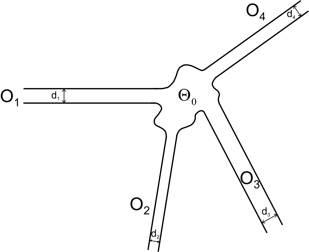
Figure 1. multi-channel domain

Solvability of stochastic Navier-Stokes equations in unbounded channel-like domains with non-zero flux condition have remained as an open problem in both two and three-dimensions. To the best of the authors knowledge, this work appears to be the first systematic treatment of stochastic two-dimensional Navier-Stokes equations in such domains. In this paper we consider a stochastic version of the problem of type (i) in multi-channel domains in two dimensions and prove a unique solvability theorem with a possible future extension to three dimensions (up to a stopping time determined by the size of the flux and the Reynolds number). The problem of type (ii) may possibly be resolved by suitably choosing a conformal mapping (see Amick and Franenkel [6] for similar ideas in the case of steady flows) to straighten the diverging outlets.

Let us consider the unbounded multi-channel domains, with several outlets as shown in the figure (see Figure 1). Let the outlets of the multi-channel domain be named as $\mathbf{O}_{1},\mathbf{O}_{2},\cdots,\mathbf{O}_{N}$ and outside a compact region let the outlets be of constant widths $d_{1},d_{2},\cdots,d_{N}$. Our first step is to construct a basic vector field through each of these outlets with the stochastic flux $\mathscr{F}_{i}(t,\omega)$ such that $\sum_{i=1}^{N}\mathscr{F}_{i}(t,\omega)=0$, $\mathbb{P}$ - a. s. The methodology of proof can be understood by considering a channel with two outlets having a unit width connected in a smooth way $\Theta=\mathbf{O}_{1}\cup\mathbf{O}_{2}\cup\Theta_{0}$ (see Figure 2).

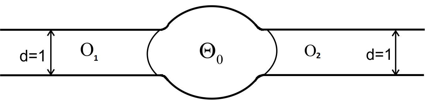
Figure 2. channel with two outlets having unit width

Let us now discuss the problems of type (i) and examine the difficulties that arise in proving solvability. The time-dependent Navier-Stokes problem is usually treated using the method of Hopf [31] in the deterministic setting which relies on $\mathrm{L}^{2}$-energy estimates. The traditional methods of solvability fail in the absence of an energy inequality. For channels of finite cross section, as pointed out in Sritharan [62], in order for the net flux to be nontrivial, the velocity field should not decay to zero at infinity (upstream and downstream) and hence such velocity fields would then have infinite energy.

Below we give a heuristic argument regarding the infinite energy of such velocity fields. We also point out that in the absence of a rigorous decay theory, only a heuristic argument could be made in this regard.

Let the velocity field be stochastic and modeled on a complete probability space ($\Omega,\mathcal{F},\mathcal{F}_{t},\mathbb{P}$). If the stochastic net flux of the velocity field $\mathbf{u}$ is $\mathscr{F}(t,\omega)$, $\omega\in\Omega$, then across any cross section $\Gamma$, we have

$$\int_{\Gamma}\mathbf{u}\cdot\mathbf{n}\/\mathrm{d}\/S=\mathscr{F}(t,\omega),$$

where $\mathbf{n}$ is the normal to the curve $\Gamma$ and $\/\mathrm{d}\/S$ is the length element.

In this case, the velocity $|\mathbf{u}(\mathbf{x},t,\omega)|\nrightarrow 0$ as $|x|\to\infty$, (where $\mathbf{x}=(x,y)$ with $y$ is of constant width) $\mathbb{P}$-a. s. To see this let us take the $2$-D case with the outlet $\mathbf{O}_{2}=\left\{(x,y)\in(0,\infty)\times(0,1)\right\}$. The flux across any cross section is same throughout the channel, due to divergence free condition. That is, if $|\mathbf{u}(\mathbf{x},t,\omega)|\to 0$ as $x\to\infty$, then the flux at the far field is zero. Hence the flux across any cross section is zero throughout the channel giving the net flux is zero. Thus for the flux to be non-zero, we need the condition that $|\mathbf{u}(\mathbf{x},t,\omega)|\nrightarrow 0$ as $x\to\infty$.

As an example, we consider the decay of $\mathbf{u}(x,y,t,\omega)$ in the following form

$$\mathbf{u}(x,y,t,\omega)\sim\frac{C_{1}(y,t,\omega)}{|x|^{\alpha}}+C_{2}(y,t,\omega),\alpha>1$$

for sufficiently large $M$ with $|x|>M$, where $C_{1}(y,t,\omega)$ and $C_{2}(y,t,\omega)>0$ be $\mathrm{L}^{2}(\Omega;C(0,T;\mathrm{L}^{2}(0,1)))$ functions such that

$$\int_{0}^{1}C_{1}(y,t,\omega)\/\mathrm{d}\/y=0\textrm{ and }\int_{0}^{1}C_{2}(y,t,\omega)\/\mathrm{d}\/y=\mathscr{F}(t,\omega).$$

From above, we have $\mathbf{u}(x,y,t,\omega)$ is flux carrying in the far field as

$$\int_{0}^{1}\mathbf{u}(x,y,t,\omega)\/\mathrm{d}\/y\sim\int_{0}^{1}\frac{C_{1}(y,t,\omega)}{|x|^{\alpha}}\/\mathrm{d}\/y+\int_{0}^{1}C_{2}(y,t,\omega)\/\mathrm{d}\/y=\mathscr{F}(t,\omega).$$

Then at any given time $t\in(0,T]$, the $\mathrm{L}^{2}$-energy is given by

$$\int_{0}^{1}\int_{0}^{\infty}|\mathbf{u}(x,y,t,\omega)|^{2}\/\mathrm{d}\/x\/\mathrm{d}\/y\geq\int_{0}^{1}\int_{M}^{\infty}|\mathbf{u}(x,y,t,\omega)|^{2}\/\mathrm{d}\/x\/\mathrm{d}\/y$$

$$\sim\int_{0}^{1}\int_{M}^{\infty}\left|\frac{C_{1}(y,t,\omega)}{|x|^{\alpha}}+C_{2}(y,t,\omega)\right|^{2}\/\mathrm{d}\/x\/\mathrm{d}\/y$$

$$=\int_{0}^{1}\int_{M}^{\infty}\frac{|C_{1}(y,t,\omega)|^{2}}{|x|^{2\alpha}}\/\mathrm{d}\/x\/\mathrm{d}\/y+\int_{0}^{1}\int_{M}^{\infty}|C_{2}(y,t,\omega)|^{2}\/\mathrm{d}\/x\/\mathrm{d}\/y$$

$$\quad+2\int_{0}^{1}\int_{M}^{\infty}\frac{C_{1}(y,t,\omega)C_{2}(y,t,\omega)}{|x|^{\alpha}}\/\mathrm{d}\/x\/\mathrm{d}\/y.$$ (1.1)

The first integral in (1) always has a finite positive value and is equal to

$$\frac{1}{(2\alpha-1)M^{2\alpha-1}}\left(\int_{0}^{1}|C_{1}(y,t,\omega)|^{2}\/\mathrm{d}\/y\right).$$

The second integral diverges to $+\infty$. The last integral in (1) is also bounded, since

$$\left|\int_{0}^{1}\int_{M}^{\infty}\frac{C_{1}(y,t,\omega)C_{2}(y,t,\omega)}{|x|^{\alpha}}\/\mathrm{d}\/x\/\mathrm{d}\/y\right|$$

$$\leq\int_{0}^{1}\int_{M}^{\infty}\frac{|C_{1}(y,t,\omega)||C_{2}(y,t,\omega)|}{|x|^{\alpha}}\/\mathrm{d}\/x\/\mathrm{d}\/y$$

$$\leq\frac{1}{(\alpha-1)M^{\alpha-1}}\left(\int_{0}^{1}|C_{1}(y,t,\omega)|^{2}\/\mathrm{d}\/y\right)^{1/2}\left(\int_{0}^{1}|C_{2}(y,t,\omega)|^{2}\/\mathrm{d}\/y\right)^{1/2}.$$

Thus for any given time $t>0$, we have

$$\int_{0}^{1}\int_{0}^{\infty}|\mathbf{u}(x,y,t,\omega)|^{2}\/\mathrm{d}\/x\/\mathrm{d}\/y=\infty,\mathbb{P}-\textrm{ a. s.}$$

There are extensive literature on deterministic flow through channel type domains. Interested readers may look into Amick [4, 5], Amick and Franenkel [6], Babin [7, 8], Borchers and Pileckas [12], Heywood [28, 29, 30], Kapitanskiì and Piletskas [32], Ladyzhenskaya and Solonnikov [37, 38, 39], Pileckas [52], Piletskas [53], Solonnikov [59], Solonnikov and Piletskas [60], Sritharan [61, 62] to name a few.

For a sample of literature on stochastic Navier-Stokes equations, we refer the readers to Bensoussan [9], Bensoussan and Temam [11], Capinski and Cutland [14], Da Parto and Zabczyk [18], Flandoli and Gatarek [24], Menaldi and Sritharan [47], Pardoux [50], [51], Sritharan and Sundar [65], Vishik and Fursikov [68], Sritharan [64], Fernando and Sritharan [23], Sakthivel and Sritharan [55].

The plan of the paper is as follows. In section 2, the main result of this paper and the functional setting have been given. A divergence free vector field of infinite energy carrying a nontrivial net flux through the channel is constructed in section 3 using the solution of the heat equation. In section 4, we characterize the properties of the linear and bilinear operators that are associated with the Navier-Stokes problem. A perturbed vector field is constructed in section 5 using a suitable transformation involving the constructed basic vector field. A-priori estimates for the solutions of the perturbed vector field are obtained in section 6. In section 7, we prove the local monotonicity condition for the sum of the Stokes and the inertia operators as well as the existence and uniqueness of strong solutions to the perturbed vector field by exploiting this local monotonicity condition. In section 8, we mathematically characterize the perturbation pressure field using a generalization of the de Rham’s Theorem to processes. section 9, completes the proof of the main result.

2. Basic Definitions and the Main Theorem

In this section, following Sritharan [62], we define the class of channel domains that will be analyzed.

Definition 2.1.

(Admissible channel domain) A simply connected open set $\Theta\subset\mathbb{R}^{2}$ with $C^{\infty}$ boundary $\partial\Theta$ consisting of two disconnected components $\partial\Theta_{1}$ and $\partial\Theta_{2}$ is called an admissible channel domain (see Figure 3), if it is the union of three disjoint sets $\Theta_{0}\cup\mathbf{O}_{1}\cup\mathbf{O}_{2}$ defined in the following way. Let $\mathbf{O}_{1}$ and $\mathbf{O}_{2}$ be two semi-infinite strips of width $d_{1}$ and $d_{2}$ respectively. These two straight channels are smoothly (not necessarily coaxially) joined by a bounded domain $\Theta_{0}$ such that $\partial\Theta_{1}\cup\partial\Theta_{2}=\partial\Theta\in C^{\infty}.$

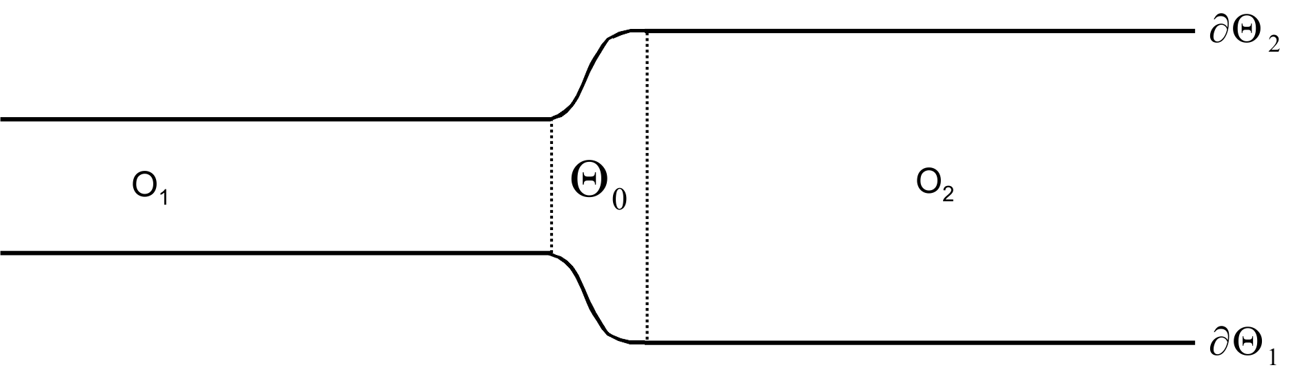
Figure 3. admissible channel domain

Now let us consider the problem of accelerating a viscous incompressible fluid from rest to a given stochastic flux rate through an admissible channel domain. Let $\left(\Omega,\mathcal{F},\mathcal{F}_{t},\mathbb{P}\right)$ be a complete probability space. The mathematical problem is to find the velocity field $\mathbf{u}$ and pressure field $p$ such that

$$(\mathbf{u},p):\Theta\times[0,T]\times\Omega\rightarrow\mathbb{R}^{2}\times\mathbb{R},$$

the momentum equation

$$\mathbf{u}_{t}+\mathbf{u}\cdot\nabla\mathbf{u}=-\nabla p+\nu\Delta\mathbf{u}+\dot{\mathscr{G}}(\mathbf{x},t,\omega)\textrm{ in }\Theta\times(0,T)\times\Omega,$$ (2.2)

the incompressibility condition

$$\nabla\cdot\mathbf{u}=0\textrm{ in }\Theta\times(0,T)\times\Omega,$$ (2.3)

the non-slip boundary condition on the channel walls

$$\mathbf{u}(\mathbf{x},t,\omega)=0\textrm{ on }\partial\Theta\times[0,T]\times\Omega,$$ (2.4)

the initial condition

$$\mathbf{u}(\mathbf{x},0,\omega)=0,\;\;(\mathbf{x},\omega)\in\Theta\times\Omega,$$ (2.5)

and the flux condition

$$\int_{\Gamma}\mathbf{u}\cdot\mathbf{n}\/\mathrm{d}\/S=\mathscr{F}(t,\omega),\textrm{ for all }t\in[0,T]\textrm{ with }\mathscr{F}(0,\omega)=0,\;\forall\;\omega\in\Omega,$$ (2.6)

are satisfied. The properties of the stochastic flux will be discussed in the later sections. Here $\nu>0$ is the coefficient of kinematic viscosity and $\Gamma$ is any cross-sectional curve cutting the channel.

In this formulation the stochasticity of fluid flow is due to an external random forcing and the random flux. Also we will assume that the external random forcing $\dot{\mathscr{G}}(\mathbf{x},t,\omega)$ and the random flux $\mathscr{F}(t,\omega)$ are mutually independent processes. Further details about the noise have been provided in the subsequent sections.

Now let us state the main result of this paper.

Theorem 2.2.

Suppose that the flux rate satisfies the moment bound:

$$\mathbb{E}\left(\int_{0}^{T}\left|\frac{\partial}{\partial t}\mathscr{F}(t,\omega)\right|^{2}\/\mathrm{d}\/t\right)\leq C_{1}(T),$$ (2.7)

for some prescribed $T$. Then for each such $\mathscr{F}(\cdot,\omega)$ there exits a unique strong solution $\mathbf{u}(\mathbf{x},t,\omega)$ with the following estimates:

$$\mathbb{E}\left(\sup_{0\leq t\leq T}\int_{\Theta}\left|(\mathbf{u}-\mathbf{w})(\mathbf{x},t,\cdot)\right|^{2}\/\mathrm{d}\/\mathbf{x}+2\nu\int_{0}^{T}\int_{\Theta}|\nabla(\mathbf{u}-\mathbf{w})(\mathbf{x},t,\cdot)|^{2}\/\mathrm{d}\/\mathbf{x}\/\mathrm{d}\/t\right)$$

$$\qquad\qquad\qquad\leq C\left(T,\nu,\int_{0}^{T}\mathrm{Tr}(g^{*}g)(t)\/\mathrm{d}\/t\right),$$ (2.8)

for some divergence free vector field $\mathbf{w}(\mathbf{x},t,\omega)$ that vanishes on the boundary $\partial\Theta$ and carries the prescribed flux

$$\int_{\Gamma}\mathbf{u}\cdot\mathbf{n}\/\mathrm{d}\/S=\int_{\Gamma}\mathbf{w}\cdot\mathbf{n}\/\mathrm{d}\/S=\mathscr{F}(t,\omega),\;\forall\;\omega\in\Omega.$$ (2.9)

We prove the above theorem in the subsequent sections. The following functional frame work is used in this paper.

$$C_{0}^{\infty}(\Theta) =\textrm{ the space of all infinitely differentiable vector fields with }$$

$$\textrm{\quad\quad compact support in }\Theta,$$

$$W_{0}(\Theta) =\textrm{ the completion of }C_{0}^{\infty}(\Theta)\textrm{ vector fields in the norm }\|\nabla\varphi\|_{\mathrm{L}^{2}(\Theta)},$$

$$H^{1}(\Theta) =\left\{\varphi:\Theta\rightarrow\mathbb{R}^{2};\;\varphi\in\mathrm{L}^{2}(\Theta),\;\nabla\varphi\in\mathrm{L}^{2}(\Theta)\right\}\!\!,$$

$$H_{0}^{1}(\Theta) =\left\{\varphi:\Theta\rightarrow\mathbb{R}^{2};\;\varphi\in\mathrm{L}^{2}(\Theta),\;\nabla\varphi\in\mathrm{L}^{2}(\Theta)\;\mathrm{and}\;\varphi\big{|}_{\partial\Theta}=0\right\}\!\!,$$

$$j(\Theta) =\left\{\varphi:\Theta\rightarrow\mathbb{R}^{2};\;\varphi\in C_{0}^{\infty}(\Theta)\;\mathrm{and}\;\nabla\cdot\varphi=0\right\}\!.$$

Also let us define

$$\mathbf{H} =\textrm{Completion of }j(\Theta)\textrm{ in the }\mathrm{L}^{2}(\Theta)\textrm{ norm},$$

$$\mathbf{V} =\textrm{Completion of }j(\Theta)\textrm{ in the }H^{1}(\Theta)\textrm{ norm},$$

$$\mathbf{H}^{*} =\left\{\varphi:\Theta\rightarrow\mathbb{R}^{2};\;\varphi\in\mathrm{L}^{2}(\Theta);\;\nabla\cdot\varphi=0\textrm{ and }\varphi\cdot\mathbf{n}\big{|}_{\partial\Theta}=0\right\}\!\!,$$

$$\mathbf{V}^{*} =\left\{\varphi:\Theta\rightarrow\mathbb{R}^{2};\;\varphi\in H_{0}^{1}(\Theta);\textrm{ and }\nabla\cdot\varphi=0\right\}\!\!,$$

$$\mathbf{V}_{0} =\textrm{completion of }j(\Theta)\textrm{ in the norm of }\|\nabla\varphi\|_{\mathrm{L}^{2}(\Theta)},$$

$$\mathbf{V}_{0}^{*} =\left\{\varphi\in W_{0}(\Theta);\nabla\cdot\varphi=0\right\}\!.$$

Let us denote the norm in $\mathbf{H}$ by $|\cdot|$ and the norm in $\mathbf{V}$ by $\|\cdot\|$. If we identify $\mathbf{H}$ with its dual $\mathbf{H}^{\prime}=\mathscr{L}(\mathbf{H};\mathbb{R})$ using the Riesz representation theorem, we obtain the continuous and dense embedding

$$\mathbf{V}\subset\mathbf{H}\equiv\mathbf{H}^{\prime}\subset\mathbf{V}^{\prime}.$$

Also let us denote the duality pairing between $\mathbf{V}$ and $\mathbf{V}^{\prime}$ by $(\cdot,\cdot)$. Note, however, that (unlike in bounded domains) the embedding $\mathbf{V}\subset\mathbf{H}$ is not compact since $\Theta$ is unbounded. Poincaré lemma holds for admissible channel domains (since they have finite cross section):

$$\|\phi\|_{\mathrm{L}^{2}(\Theta)}\leq C\|\nabla\phi\|_{\mathrm{L}^{2}(\Theta)},\quad\forall\phi\in H^{1}_{0}(\Theta)$$

and hence, in $\mathbf{V}$ the norm of $H^{1}(\Theta)$ is equivalent to that obtained by the Dirichlet integral $\|\nabla\phi\|_{\mathrm{L}^{2}(\Theta)}.$

3. Construction of the Basic Vector Field

Following the ideas from Sritharan [62], we will construct a divergence free basic vector field $\mathbf{w}(\mathbf{x},t,\omega)$ in $\Theta$ which vanishes on $\partial\Theta$ and carries the prescribed random flux $\mathscr{F}(t,\omega)$ through the channel. Note that this “constructed” vector field need not satisfy the Navier-Stokes equations in $\Theta$ although it does in $\mathbf{O}_{1}$ and $\mathbf{O}_{2}$ due to the nature of the construction used. The method can be described as follows. Using the solution of the one-dimensional heat equation with random flux $\mathscr{F}(t,\omega)$, a vector field is constructed in each of the straight channel outlets $\mathbf{O}_{1}$ and $\mathbf{O}_{2}$. We then smoothly join these two vector fields by constructing a smooth extension in $\Theta_{0}$. In $\mathbf{O}_{1}$ and $\mathbf{O}_{2}$ the vector field will have only one component, namely in the direction of the axes of the outlets. In $\Theta_{0}$, however, in general both components of $\mathbf{w}(\mathbf{x},t,\omega)$ will be nonzero. Let us now consider one of the outlets, say $\mathbf{O}_{2}$ and assume for simplicity that the width of the channel is unity (see Figure 4).

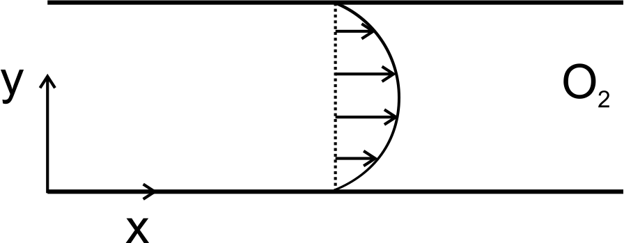
Figure 4. The outlet $\mathbf{O}_{2}$

Let us define the outlet $\mathbf{O}_{2}=\left\{(x,y)\in(0,\infty)\times(0,1)\right\}.$ Let us seek a divergence-free vector field in the form $\mathbf{w}(x,y,t,\omega)=(w_{1}(y,t,\omega),0)$ and a scalar field $P(x,t,\omega)$ in $\mathbf{O}_{2}$ such that

$$\frac{\partial}{\partial t}w_{1}(y,t,\omega)-\nu\frac{\partial^{2}}{\partial y^{2}}w_{1}(y,t,\omega) =-\frac{\partial}{\partial x}P(x,t,\omega)=f(t,\omega)$$

$$\quad\textrm{ in }\mathbf{O}_{2}\times(0,T)\times\Omega,$$ (3.1)

$$w_{1}(0,t,\omega)=w_{1}(1,t,\omega) =0\textrm{ for }t\in[0,T],\omega\in\Omega,$$ (3.2)

$$w_{1}(y,0,\omega) =0\textrm{ for }y\in(0,1),\omega\in\Omega\textrm{ and }$$ (3.3)

$$\int_{0}^{1}w_{1}(y,t,\omega)\/\mathrm{d}\/y=\mathscr{F}(t,\omega)\textrm{ for }t\in[0,T]\textrm{ with }\mathscr{F}(0,\omega)=0\;\forall\;\omega\in\Omega.$$ (3.4)

Here the function $f(t,\omega)$ needs to be determined from the prescribed flux $\mathscr{F}(t,\omega)$. To resolve this problem we first write down the solution of the system (3)-(3.3) in terms of $f(t,\omega)$ and then use the condition (3.4) to evaluate $f(t,\omega)$ in terms of $\mathscr{F}(t,\omega)$. The solution of (3)-(3.3) can be obtained by the method of separation of variables (see Cannon [17]). The existence and uniqueness of solution of the boundary value problem for the heat equation with stochastic boundary conditions has been proved in Cahlon [16].

Theorem 3.1.

Let $f(t,\omega)$ satisfies the following uniform Hölder condition on $[0,T]$, for all $t_{1},t_{2}\in[0,T]$,

$$|f(t_{1},\omega)-f(t_{2},\omega)|\leq L(\omega)|t_{1}-t_{2}|^{\gamma},0<\gamma<\frac{1}{2},$$ (3.5)

with $L(\omega)>0$ and $L(\cdot)\in\mathrm{L}^{2}(\Omega)$. Then, there exists a unique solution $w_{1}(\cdot,\cdot,\cdot)$ of the problem (3)-(3.3) such that

$$w_{1}(y,t,\omega)\in\mathrm{L}^{2}\left(\Omega;C([0,1]\times[0,T])\right)$$

and satisfying the following conditions.

1. $w_{1}(y,t,\omega)$ is a continuous function of $y$ and $t$ in $\mathrm{L}^{2}(\Omega)$. i.e.,

   $$\mathbb{E}\left[\left(w_{1}(y,t+h,\omega)-w_{1}(y,t,\omega)\right)^{2}\right]\to 0\textrm{ as }h\to 0,$$

   $$\mathbb{E}\left[\left(w_{1}(y+h,t,\omega)-w_{1}(y,t,\omega)\right)^{2}\right]\to 0\textrm{ as }h\to 0.$$ (3.6)

2. There exists a stochastic function $w_{1_{t}}(y,t,\omega)\in\mathrm{L}^{2}(\Omega;C([0,1]\times[0,T]))$ such that

   $$\mathbb{E}\left[\left(\frac{w_{1}(y,t+h,\omega)-w_{1}(y,t,\omega)}{h}-w_{1_{t}}(y,t,\omega)\right)^{2}\right]\to 0\textrm{ as }h\to 0.$$ (3.7)

3. There exists a stochastic function $w_{1_{yy}}(y,t,\omega)\in\mathrm{L}^{2}(\Omega;C([0,1]\times[0,T]))$ such that

   $$\mathbb{E}\left[\left(\frac{w_{1}(y+h,t,\omega)+w_{1}(y-h,t,\omega)-2w_{1}(y,t,\omega)}{h^{2}}-w_{1_{yy}}(y,t,\omega)\right)^{2}\right]$$

   $$\to 0\textrm{ as }h\to 0.$$ (3.8)

4. The equation $w_{1_{t}}(y,t,\omega)=\nu w_{1_{yy}}(y,t,\omega)+f(t,\omega)$ is satisfied for a. e. $\omega\in\Omega$.

Proof.

By using the method of separation of variables, we can write down the solution of (3)-(3.3) as

$$w_{1}(y,t,\omega)=\frac{4}{\pi}\sum_{n=0}^{\infty}\left\{\int_{0}^{t}f(s,\omega)\frac{1}{2n+1}e^{(-\nu(2n+1)^{2}\pi^{2}(t-s))}\/\mathrm{d}\/s\right\}\sin(2n+1)\pi y.$$ (3.9)

We now use the Weierstrass’ M-test to show that the infinite series solution (3.9) to the Heat Equation (3)-(3.3) converges uniformly. Let us take

$$a_{n}(y,t,\omega)=\int_{0}^{t}f(s,\omega)\frac{1}{2n+1}e^{(-\nu(2n+1)^{2}\pi^{2}(t-s))}\/\mathrm{d}\/s\sin(2n+1)\pi y,\textrm{ for }t>0.$$

Then by using Hölder’s inequality, for $t\in(0,T]$ and $y\in[0,1]$, we have

$$|a_{n}(y,t,\omega)| \leq\int_{0}^{t}|f(s,\omega)|\frac{1}{2n+1}e^{(-\nu(2n+1)^{2}\pi^{2}(t-s))}\/\mathrm{d}\/s$$

$$\leq\frac{1}{(2n+1)}e^{-\nu(2n+1)^{2}\pi^{2}t}\left(\int_{0}^{t}|f(s,\omega)|^{2}\/\mathrm{d}\/s\right)^{1/2}\left(\int_{0}^{t}e^{2\nu(2n+1)^{2}\pi^{2}s}\/\mathrm{d}\/s\right)^{1/2}$$

$$\leq\|f(\cdot,\omega)\|_{\mathrm{L}^{2}(0,T)}\frac{1}{(2n+1)}e^{-\nu(2n+1)^{2}\pi^{2}t}\left(\frac{e^{2\nu(2n+1)^{2}\pi^{2}t}-1}{2\nu(2n+1)^{2}\pi^{2}}\right)^{1/2}$$

$$\leq\|f(\cdot,\omega)\|_{\mathrm{L}^{2}(0,T)}\frac{1}{(2n+1)^{2}\pi\sqrt{2\nu}},\quad\mathbb{P}-\textrm{ a. s. }$$ (3.10)

Hence, we get

$$|a_{n}(y,t,\omega)|\leq M_{n}\textrm{ where }M_{n}=\|f(\cdot,\omega)\|_{\mathrm{L}^{2}(0,T)}\frac{1}{(2n+1)^{2}\pi\sqrt{2\nu}},\mathbb{P}-\textrm{ a. s.}$$

Since $\sum_{n=0}^{\infty}\frac{1}{(2n+1)^{2}}=\frac{\pi^{2}}{8}$ (from Apostol [2], we have $\sum_{n=1}^{\infty}\frac{1}{n^{2}}=\frac{\pi^{2}}{6}$, then $\sum_{n=1}^{\infty}\frac{1}{(2n)^{2}}+\sum_{n=0}^{\infty}\frac{1}{(2n+1)^{2}}=\frac{\pi^{2}}{6}$ gives $\sum_{n=0}^{\infty}\frac{1}{(2n+1)^{2}}=\frac{\pi^{2}}{8}$), we have $\sum_{n=0}^{\infty}M_{n}=\frac{\pi}{8\sqrt{2\nu}}\|f(\cdot,\omega)\|_{\mathrm{L}^{2}(0,T)}$, $\mathbb{P}$- a. s., for all $t\in(0,T]$. Hence by the Weierstrass’ M-test, $w_{1}(y,t,\omega)=\frac{4}{\pi}\sum_{n=0}^{\infty}a_{n}(y,t,\omega)$ converges absolutely and uniformly for $y\in[0,1]$ and $t>0$. For $t=0$ also the convergence is uniform since $w_{1}(y,0,\omega)=0$.

One can re-write (3.9) as

$$w_{1}(y,t,\omega)=\int_{0}^{t}K(y,t-s)f(s,\omega)\/\mathrm{d}\/s=(K*f)(t),$$ (3.11)

where

$$K(y,t)=\frac{4}{\pi}\sum_{n=0}^{\infty}\frac{1}{(2n+1)}e^{-\nu(2n+1)^{2}\pi^{2}t}\sin(2n+1)\pi y.$$

From (3.5), we have

$$\mathbb{E}\left[|f(t_{1},\omega)-f(t_{2},\omega)|^{2}\right] \leq\mathbb{E}\left[L(\omega)|t_{1}-t_{2}|^{\gamma}\right]^{2}$$

$$=\mathbb{E}|L(\omega)|^{2}|t_{1}-t_{2}|^{2\gamma}\to 0\textrm{ as }t_{1}\to t_{2},$$

for all $t_{1},t_{2}\in[0,T]$, which gives $f(\cdot,\cdot)\in\mathrm{L}^{2}(\Omega;C[0,T]).$ We can prove that the solution (3.9) of the problem (3)-(3.3) satisfies $w_{1}(y,t,\omega)\in\mathrm{L}^{2}\left(\Omega;C([0,1]\times[0,T])\right)$ (see Cahlon [16] and Walsh [69] for existence and uniqueness).

Let us now prove part (iv) of the theorem. For $t>0$, we have

$$\frac{\partial}{\partial t}(w_{1}(y,t,\omega)) =\frac{\partial}{\partial t}\left[\int_{0}^{t}K(y,t-s)f(s,\omega)\/\mathrm{d}\/s\right]$$

$$=\frac{\partial}{\partial t}\left[\int_{0}^{\infty}H(t-s)K(y,t-s)f(s,\omega)\/\mathrm{d}\/s\right]$$

$$=\int_{0}^{\infty}\left[H(t-s)\frac{\partial}{\partial t}K(y,t-s)+K(y,t-s)\delta(t-s)\right]f(s,\omega)\/\mathrm{d}\/s$$

$$=\int_{0}^{t}\frac{\partial}{\partial t}K(y,t-s)f(s,\omega)\/\mathrm{d}\/s+\frac{4}{\pi}\sum_{n=0}^{\infty}\frac{\sin(2n+1)\pi y}{(2n+1)}f(t,\omega)$$

$$=\int_{0}^{t}\frac{\partial}{\partial t}K(y,t-s)f(s,\omega)\/\mathrm{d}\/s+f(t,\omega),$$ (3.12)

where $H(\cdot)$ is the Heaviside function. The last term is obtained by using the property of $\delta$-function and using the formula $\sum_{n=0}^{\infty}\frac{\sin(2n+1)\pi y}{(2n+1)}=\frac{\pi}{4}$, for $y\in(0,1)$. By a direct calculation, as $K(\cdot,\cdot)$ is uniformly convergent in time $t>0$ for a fixed $y\in(0,1)$, it is easy to see that

$$\frac{\partial}{\partial t}K(y,t-s)=-4\nu\pi\sum_{n=0}^{\infty}(2n+1)e^{-\nu(2n+1)^{2}\pi^{2}(t-s)}\sin(2n+1)\pi y.$$

From (3), using the uniform convergence of the above series in time $t>0$ for a fixed $y\in(0,1)$, we have

$$\frac{\partial}{\partial t}(w_{1}(y,t,\omega)) =-4\nu\pi\sum_{n=0}^{\infty}\left\{\int_{0}^{t}\left[(2n+1)e^{-\nu(2n+1)^{2}\pi^{2}(t-s)}f(s,\omega)\right]\/\mathrm{d}\/s\times\right.$$

$$\quad\sin(2n+1)\pi y\Big{\}}+f(t,\omega).$$ (3.13)

Next, let us calculate $\frac{\partial^{2}}{\partial y^{2}}w_{1}(y,t,\omega)$. We have

$$\frac{\partial^{2}}{\partial y^{2}}w_{1}(y,t,\omega)=\int_{0}^{t}\frac{\partial^{2}}{\partial y^{2}}[K(y,t-s)]f(s,\omega)\/\mathrm{d}\/s.$$ (3.14)

Since $K(\cdot,\cdot)$ is uniformly convergent in $y$ and $\frac{\partial K}{\partial t}(\cdot,\cdot)$ is also uniformly convergent in $y$ for a fixed $t>0$, by a simple calculation, we have

$$\frac{\partial^{2}}{\partial y^{2}}[K(y,t-s)]=-4\pi\sum_{n=0}^{\infty}(2n+1)e^{-\nu(2n+1)^{2}\pi^{2}(t-s)}\sin(2n+1)\pi y.$$

The above series is uniformly convergent in time $t>0$ for a fixed $y\in(0,1)$ and hence from (3.14), we get

$$\frac{\partial^{2}w_{1}}{\partial y^{2}}=-4\pi\sum_{n=0}^{\infty}\int_{0}^{t}(2n+1)e^{-\nu(2n+1)^{2}\pi^{2}(t-s)}f(s,\omega)\sin(2n+1)\pi y\/\mathrm{d}\/s.$$ (3.15)

The above integral is well defined and from equations (3) and (3.15), we have part (iv) of the theorem.

Now we prove part (i) of the theorem. Since $K$ is continuous in time $t$, for any given $\varepsilon>0$, there exists a $\eta>0$ such that

$$\left|K(y,t_{1})-K(y,t_{2})\right|<\varepsilon\textrm{ whenever }|t_{1}-t_{2}|<\eta,$$

$t_{1},t_{2}\in(0,T]$. For $f(\cdot,\cdot)\in\mathrm{L}^{2}(\Omega;C[0,T])$, by choosing $|h|<\eta$, let us consider $\mathbb{E}\left[w_{1}(y,t+h,\omega)-w_{1}(y,t,\omega)\right]^{2}$ and by using Young’s inequality and continuity of $K(y,t)$ in $t$, we have

$$\mathbb{E}\left[w_{1}(y,t+h,\omega)-w_{1}(y,t,\omega)\right]^{2}$$

$$=\mathbb{E}\left(\int_{0}^{t+h}K(y,t+h-s)f(s,\omega)\/\mathrm{d}\/s-\int_{0}^{t}K(y,t-s)f(s,\omega)\/\mathrm{d}\/s\right)^{2}$$

$$\leq 2\mathbb{E}\left(\int_{0}^{t}\left|K(y,t+h-s)-K(y,t-s)\right|^{2}|f(s,\omega)|^{2}\/\mathrm{d}\/s\right)$$

$$\quad+2\mathbb{E}\left(\int_{t}^{t+h}|K(y,t+h-s)|^{2}|f(s,\omega)|^{2}\/\mathrm{d}\/s\right)$$

$$\leq 2\mathbb{E}\left[\sup_{0\leq s\leq t}|f(s,\omega)|^{2}\right]\int_{0}^{t}|K(y,t+h-s)-K(y,t-s)|^{2}\/\mathrm{d}\/s$$

$$\quad+2\mathbb{E}\left[\sup_{0\leq s\leq t}|f(s,\omega)|^{2}\right]\int_{t}^{t+h}|K(y,t+h-s)|^{2}\/\mathrm{d}\/s$$

$$\leq 2\|f\|^{2}_{\mathrm{L}^{2}(\Omega;C[0,T])}\left(\varepsilon^{2}T+\int_{t}^{t+h}|K(y,t+h-s)|^{2}\/\mathrm{d}\/s\right)\to 0\textrm{ as }h\to 0,$$

since $\varepsilon$ is arbitrary and as $h\to 0$, $t\to s$ and $K(y,t+h-s)\to K(y,0)=1$ for all $y\in(0,1)$. Similarly, $\mathbb{E}(w_{1}(y+h,t,\omega)-w_{1}(y,t,\omega))^{2}\to 0\textrm{ as }h\to 0.$

Let us now prove part (ii) of the theorem. Since for a fixed $y\in(0,1)$, $K(y,t)$ is uniformly convergent in time $t>0$ and its derivative $\frac{\partial K}{\partial t}$ exists and also is uniformly convergent for $t>0$, we have for a given $\varepsilon>0$, there exists an $\eta>0$ such that

$$\left|\frac{K(y,t+h)-K(y,t)}{h}-\frac{\partial}{\partial t}K(y,t)\right|<\varepsilon\textrm{ when ever }|h|<\eta.$$

To prove (3.7), let us use the differentiability of $K(y,t)$ in time $t$. For $|h|<\eta$, we have

$$\mathbb{E}\left[\left(\frac{w_{1}(y,t+h,\omega)-w_{1}(y,t,\omega)}{h}-w_{1_{t}}(y,t,\omega)\right)^{2}\right]$$

$$=\mathbb{E}\left[\int_{0}^{t}\left(\frac{K(y,t+h-s)-K(y,t-s)}{h}\right)f(s,\omega)\/\mathrm{d}\/s\right.$$

$$\left.\quad+\frac{1}{h}\int_{t}^{t+h}K(y,t+h-s)f(s,\omega)\/\mathrm{d}\/s-\int_{0}^{t}\frac{\partial}{\partial t}K(y,t-s)f(s,\omega)\/\mathrm{d}\/s-f(t,\omega)\right]^{2}$$

$$\leq 2\mathbb{E}\left[\sup_{0\leq s\leq t}|f(s,\omega)|^{2}\right]\int_{0}^{t}\left|\frac{K(y,t+h-s)-K(y,t-s)}{h}-\frac{\partial}{\partial t}K(y,t-s)\right|^{2}\/\mathrm{d}\/s$$

$$\quad+2\mathbb{E}\left(\frac{1}{h}\int_{t}^{t+h}\left[K(y,t+h-s)f(s,\omega)-f(t,\omega)\right]\/\mathrm{d}\/s\right)^{2}$$

$$\leq 2\|f\|^{2}_{\mathrm{L}^{2}(\Omega;C[0,T])}\varepsilon^{2}T+2\mathbb{E}\left(\frac{1}{h}\int_{t}^{t+h}\left[K(y,t+h-s)f(s,\omega)-f(t,\omega)\right]\/\mathrm{d}\/s\right)^{2}.$$

Note that in the time interval $[t,t+h]$ as $h\to 0$, $s\to t$ and hence the function $K(y,t+h-s)f(s,\omega)\to K(y,0)f(t,\omega)=f(t,\omega)$. Thus by the Lebesgue’s differentiation theorem (Theorem 6, Appendix E.4 of Evans [21]), the last term of the right hand side of the above inequality goes to $0$ as $h\to 0$. Finally, since $\varepsilon>0$ is arbitrary, we have the desired result (3.7). Similarly one can prove that there exists a stochastic function $w_{1_{yy}}(y,t,\omega)\in\mathrm{L}^{2}(\Omega;C([0,1]\times[0,T]))$ such that

$$\mathbb{E}\left[\left(\frac{w_{1}(y+h,t,\omega)+w_{1}(y-h,t,\omega)-2w_{1}(y,t,\omega)}{h^{2}}-w_{1_{yy}}(y,t,\omega)\right)^{2}\right]$$

$$\to 0\textrm{ as }h\to 0.$$

∎

Corollary 3.2.

For $f(\cdot,\cdot)\in\mathrm{L}^{2}(\Omega;C[0,T])$, there exists a function $\frac{\partial}{\partial t}\mathscr{F}(\cdot,\cdot)\in\mathrm{L}^{2}(\Omega;C[0,T])$ such that

$$\frac{\partial}{\partial t}\mathscr{F}(t,\omega)=f(t,\omega)+\int_{0}^{t}\frac{\partial}{\partial t}\mathfrak{h}(t-\tau)f(\tau,\omega)\/\mathrm{d}\/\tau,$$ (3.16)

where $\mathfrak{h}(t)=\frac{8}{\pi^{2}}\sum_{n=0}^{\infty}\frac{1}{(2n+1)^{2}}\exp(-\nu(2n+1)^{2}\pi^{2}t).$

Proof.

From (3.4), we have

$$\mathscr{F}(t,\omega) =\frac{8}{\pi^{2}}\sum_{n=0}^{\infty}\left\{\int_{0}^{t}f(\tau,\omega)\frac{1}{(2n+1)^{2}}e^{(-\nu(2n+1)^{2}\pi^{2}(t-\tau))}\/\mathrm{d}\/\tau\right\}$$

$$=\int_{0}^{t}\mathfrak{h}(t-\tau)f(\tau,\omega)\/\mathrm{d}\/\tau,$$ (3.17)

where

$$\mathfrak{h}(t)=\frac{8}{\pi^{2}}\sum_{n=0}^{\infty}\frac{1}{(2n+1)^{2}}\exp(-\nu(2n+1)^{2}\pi^{2}t).$$ (3.18)

Note that since $\mathfrak{h}(t)$ is a decreasing function of $t$, we have for all $t>0,\;\mathfrak{h}(t)\leq\mathfrak{h}(0)=\frac{8}{\pi^{2}}\sum_{n=0}^{\infty}\frac{1}{(2n+1)^{2}}=1$. Also the series $\mathfrak{h}(t)$ is convergent. Then there exists a function $\frac{\partial}{\partial t}\mathscr{F}(t,\omega)\in\mathrm{L}^{2}(\Omega;C[0,T])$ such that

$$\frac{\partial}{\partial t}\mathscr{F}(t,\omega)=f(t,\omega)+\int_{0}^{t}\frac{\partial}{\partial t}\mathfrak{h}(t-\tau)f(\tau,\omega)\/\mathrm{d}\/\tau,$$ (3.19)

where $\frac{\partial}{\partial t}\mathfrak{h}(t)=-8\nu\sum_{n=0}^{\infty}e^{-\nu(2n+1)^{2}\pi^{2}t}$. Since $\mathfrak{h}$ is differentiable in time $t>0$, for any given $\varepsilon>0$, there exists an $\eta>0$ such that

$$\left|\frac{\mathfrak{h}(t+h)-\mathfrak{h}(t)}{h}-\frac{\partial}{\partial t}\mathfrak{h}(t)\right|\leq\varepsilon\textrm{ when ever }|h|<\eta.$$

For proving the existence of $\frac{\partial}{\partial t}\mathscr{F}(t,\omega)$, let us use $f\in\mathrm{L}^{2}(\Omega;C[0,T])$, the differentiability of $\mathfrak{h}$ and choose $|h|<\eta$ to get

$$\mathbb{E}\left[\frac{\mathscr{F}(t+h,\omega)-\mathscr{F}(t,\omega)}{h}-\frac{\partial}{\partial t}\mathscr{F}(t,\omega)\right]^{2}$$

$$\leq 2\mathbb{E}\left[\int_{0}^{t}\left(\frac{\mathfrak{h}(t+h-\tau)-\mathfrak{h}(t-\tau)}{h}-\frac{\partial}{\partial t}\mathfrak{h}(t-\tau)\right)f(\tau,\omega)\/\mathrm{d}\/\tau\right]^{2}$$

$$\quad+2\mathbb{E}\left[\frac{1}{h}\int_{t}^{t+h}\left[\mathfrak{h}(t+h-\tau)f(\tau,\omega)-f(t,\omega)\right]\/\mathrm{d}\/\tau\right]^{2}$$

$$\leq 2\mathbb{E}\left[\sup_{0\leq\tau\leq t}|f(\tau,\omega)|^{2}\right]\int_{0}^{t}\left|\frac{\mathfrak{h}(t+h-\tau)-\mathfrak{h}(t-\tau)}{h}-\frac{\partial}{\partial t}\mathfrak{h}(t-\tau)\right|^{2}\/\mathrm{d}\/\tau$$

$$\quad+2\mathbb{E}\left[\frac{1}{h}\int_{t}^{t+h}\left[\mathfrak{h}(t+h-\tau)f(\tau,\omega)-f(t,\omega)\right]\/\mathrm{d}\/\tau\right]^{2}$$

$$\leq 2\|f\|^{2}_{\mathrm{L}^{2}(\Omega;C[0,T])}\varepsilon^{2}T+2\mathbb{E}\left[\frac{1}{h}\int_{t}^{t+h}\left[\mathfrak{h}(t+h-\tau)f(\tau,\omega)-f(t,\omega)\right]\/\mathrm{d}\/\tau\right]^{2}.$$

Note that in the time interval $[t,t+h]$ as $h\to 0$, $s\to t$ and hence the function $\mathfrak{h}(t+h-\tau)f(\tau,\omega)\to f(t,\omega)$. Thus by the Lebesgue’s differentiation theorem (Theorem 6, Appendix E.4 of Evans [21]), the last term of the right hand side of the above inequality goes to $0$ as $h\to 0$. The arbitrariness of $\varepsilon$ gives the required result. ∎

We have

$$\frac{\partial}{\partial t}\mathscr{F}(t,\omega)=f(t,\omega)+\int_{0}^{t}\frac{\partial}{\partial t}\mathfrak{h}(t-\tau)f(\tau,\omega)\/\mathrm{d}\/\tau,$$ (3.20)

where

$$\frac{\partial}{\partial t}\mathfrak{h}(t)=-8\nu\sum_{n=0}^{\infty}e^{-\nu(2n+1)^{2}\pi^{2}t}.$$

From (3.20), denoting $\frac{\partial}{\partial t}\mathfrak{h}(t-\tau)$ as $\mathcal{H}(t-\tau)$, we obtain the Volterra integral equation of the second kind for the determination of $f(\cdot,\cdot)$ in terms of $\frac{\partial}{\partial t}\mathscr{F}(t,\omega)$,

$$f(t,\omega)=\frac{\partial}{\partial t}\mathscr{F}(t,\omega)-\int_{0}^{t}\mathcal{H}(t-\tau)f(\tau,\omega)\/\mathrm{d}\/\tau.$$ (3.21)

Lemma 3.3.

Let $\frac{\partial}{\partial t}\mathscr{F}(\cdot,\cdot)\in\mathrm{L}^{2}(\Omega;\mathrm{L}^{2}(0,T))$ be given. Then there exists a unique solution $f(\cdot,\cdot)\in\mathrm{L}^{2}(\Omega;\mathrm{L}^{2}(0,T))$ for the integral equation (3.21) in the form

$$f(t,\omega)=\sum_{n=0}^{\infty}\left[\mathscr{K}^{n}\frac{\partial\mathscr{F}}{\partial t}\right](t,\omega),$$ (3.22)

where $\mathscr{K}$ is given by

$$\left[\mathscr{K}\psi\right](t,\omega)=-\int_{0}^{t}\mathcal{H}(t-\tau)\psi(\tau,\omega)\/\mathrm{d}\/\tau=-(\mathcal{H}*\psi)(t,\omega).$$ (3.23)

Proof.

Let us begin with the convolution (3.23) and apply Young’s inequality for convolutions to obtain

$$\left\|\mathscr{K}\psi(\cdot,\cdot)\right\|^{2}_{\mathrm{L}^{2}(\Omega;\mathrm{L}^{2}(0,T))} =\mathbb{E}\left(\int_{0}^{T}\left|-\int_{0}^{t}\mathcal{H}(t-\tau)\psi(\tau,\omega)\/\mathrm{d}\/\tau\right|^{2}\/\mathrm{d}\/t\right)$$

$$=\mathbb{E}\left(\|(\mathcal{H}*\psi)(\cdot,\cdot)\|_{\mathrm{L}^{2}(0,T)}^{2}\right)$$

$$\leq\mathbb{E}\left(\|(\mathcal{H}(\cdot)\|^{2}_{\mathrm{L}^{1}(0,T)}\|\psi(\cdot,\cdot)\|_{\mathrm{L}^{2}(0,T)}^{2}\right)$$

$$=\left\|\mathcal{H}(\cdot)\right\|^{2}_{\mathrm{L}^{1}(0,T)}\mathbb{E}\left(\left\|\psi(\cdot,\cdot)\right\|_{\mathrm{L}^{2}(0,T)}^{2}\right)$$

$$=\left\|\mathcal{H}(\cdot)\right\|^{2}_{\mathrm{L}^{1}(0,T)}\left\|\psi(\cdot,\cdot)\right\|^{2}_{\mathrm{L}^{2}(\Omega;\mathrm{L}^{2}(0,T))}$$ (3.24)

Let us define

$$\rho=\left\|\mathcal{H}(\cdot)\right\|_{\mathrm{L}^{1}(0,T)}\leq\mathfrak{h}(0)-\mathfrak{h}(T)=1-\mathfrak{h}(T)<1.$$

Hence from (3), we get

$$\left\|\mathscr{K}\psi(\cdot,\cdot)\right\|_{\mathrm{L}^{2}(\Omega;\mathrm{L}^{2}(0,T))}<\rho\left\|\psi\right\|_{\mathrm{L}^{2}(\Omega;\mathrm{L}^{2}(0,T))},\;\forall\;\psi\in\mathrm{L}^{2}(\Omega;\mathrm{L}^{2}(0,T)).$$ (3.25)

Let us define the map $\mathscr{J}$ to be

$$\left[\mathscr{J}f\right](t,\omega)=\frac{\partial}{\partial t}\mathscr{F}(t,\omega)+\left[\mathscr{K}f\right](t,\omega).$$ (3.26)

Let us denote the approximate solutions of (3.21) as $f_{0},f_{1},\cdots,f_{n}$ and they are given by

$$f_{0}(t,\omega) =\frac{\partial}{\partial t}\mathscr{F}(t,\omega),$$

$$f_{1}(t,\omega) =\frac{\partial}{\partial t}\mathscr{F}(t,\omega)-\int_{0}^{t}\mathcal{H}(t-\tau)f_{0}(\tau,\omega)\/\mathrm{d}\/\tau$$

$$=\frac{\partial}{\partial t}\mathscr{F}(t,\omega)+\left[\mathcal{K}f_{0}\right](t,\omega)=\left[\mathscr{J}f_{0}\right](t,\omega)=\sum_{j=0}^{1}\left[\mathscr{K}^{j}\frac{\partial\mathscr{F}}{\partial t}\right](t,\omega),$$

$$f_{2}(t,\omega) =\frac{\partial}{\partial t}\mathscr{F}(t,\omega)-\int_{0}^{t}\mathcal{H}(t-\tau)f_{1}(\tau,\omega)\/\mathrm{d}\/\tau$$

$$=\frac{\partial}{\partial t}\mathscr{F}(t,\omega)+\left[\mathcal{K}f_{0}\right](t,\omega)+\left[\mathcal{K}^{2}f_{0}\right](t,\omega)$$

$$=\left[\mathscr{J}^{2}f_{0}\right](t,\omega)=\sum_{j=0}^{2}\left[\mathscr{K}^{j}\frac{\partial\mathscr{F}}{\partial t}\right](t,\omega),$$

$$\quad\vdots$$

$$f_{n}(t,\omega) =\frac{\partial}{\partial t}\mathscr{F}(t,\omega)+\left[\mathcal{K}f_{n-1}\right](t,\omega)=\left[\mathscr{J}f_{n-1}\right](t,\omega).$$ (3.27)

Clearly these approximations satisfy

$$f_{n}(t,\omega)=\left[\mathscr{J}^{n}f_{0}\right](t,\omega)=\sum_{j=0}^{n}\left[\mathscr{K}^{j}\frac{\partial\mathscr{F}}{\partial t}\right](t,\omega)$$ (3.28)

and

$$f_{n}(t,\omega)-f_{n-1}(t,\omega)=\left[\mathscr{K}^{n}\frac{\partial\mathscr{F}}{\partial t}\right](t,\omega).$$ (3.29)

Hence by using the estimate (3.25) on (3.29), we obtain

$$\left\|f_{n}(\cdot,\cdot)-f_{n-1}(\cdot,\cdot)\right\|_{\mathrm{L}^{2}(\Omega;\mathrm{L}^{2}(0,T))}<\rho^{n}\left\|\frac{\partial\mathscr{F}}{\partial t}\right\|_{\mathrm{L}^{2}(\Omega;\mathrm{L}^{2}(0,T))}\textrm{ with }\rho<1.$$ (3.30)

The existence of a unique fixed point $f(t,\omega)\in\mathrm{L}^{2}(\Omega;\mathrm{L}^{2}(0,T))$ to the map $\mathscr{J}$ is ensured by Banach contraction mapping theorem and using the estimate (3.30). The unique fixed point $f(t,\omega)\in\mathrm{L}^{2}(\Omega;\mathrm{L}^{2}(0,T))$ to the map $\mathscr{J}$ is such that

$$\lim_{n\to\infty}\left\|f(\cdot,\cdot)-f_{n}(\cdot,\cdot)\right\|_{\mathrm{L}^{2}(\Omega;\mathrm{L}^{2}(0,T))}=0$$ (3.31)

and

$$\left[\mathscr{J}f\right](t,\omega)=f(t,\omega)=\sum_{n=0}^{\infty}\left[\mathscr{K}^{n}\frac{\partial\mathscr{F}}{\partial t}\right](t,\omega).$$ (3.32)

∎

Let us now go back to the system (3)-(3.4) and note that a given $\frac{\partial}{\partial t}\mathscr{F}(\cdot,\cdot)\in\mathrm{L}^{2}(\Omega;\mathrm{L}^{2}(0,T))$ corresponds uniquely to a solution $w_{1}(\cdot,\cdot,\cdot)$ given by (3.9) and (3.22). Moreover, $P(\cdot,\cdot,\cdot)$ is given by

$$P(x,t,\omega)=-xf(t,\omega)+g_{1}(t,\omega),$$

for some arbitrary scalar function $g_{1}(t,\omega)$ (which can be set to zero for a. e. $\Omega$) for each $\omega\in\Omega$. The regularity of $w_{1}(\cdot,\cdot,\cdot)$ can be verified by estimating (3.9).

Let us now obtain a stochastic version of the Theorem 2 (section 3) from Sritharan [62].

Theorem 3.4.

Let $\frac{\partial}{\partial t}\mathscr{F}(\cdot,\cdot)\in\mathrm{L}^{2}(\Omega;\mathrm{L}^{2}(0,T))$ be given. Then the solution $(w_{1},P)$ of (3)-(3.4) is unique and for $0\leq\varepsilon<\frac{1}{2}$

$$w_{1}\in\mathrm{L}^{2}(\Omega;\mathrm{L}^{2}(0,T;H_{0}^{1}(0,1)\cap H^{2+\varepsilon}(0,1))\cap C([0,T];H_{0}^{1}(0,1)))$$

and

$$\partial_{t}w_{1}\in\mathrm{L}^{2}(\Omega;\mathrm{L}^{2}(0,T;H^{\varepsilon}(0,1))).$$

Proof.

We only need to verify the regularity. Let us denote by $\mathscr{A}$ the Friedrich’s extension of the operator $-\partial_{y}^{2}$ to $H_{0}^{1}(0,1)\cap H^{2}(0,1).$ Then from (3.9), by using the uniform convergence of the series solution $w_{1}(y,t,\omega)$, Fubini’s theorem and Young’s inequality for convolutions, we have

$$\mathbb{E}\left(\int_{0}^{T}\|\mathscr{A}^{1+\varepsilon/2}w_{1}(y,t,\omega)\|_{\mathrm{L}^{2}(0,1)}^{2}\/\mathrm{d}\/t\right)$$

$$=\mathbb{E}\left(\int_{0}^{T}\left\|\frac{4}{\pi}\sum_{n=0}^{\infty}\left\{\int_{0}^{t}f(\tau,\omega)\frac{1}{(2n+1)}e^{-\nu(2n+1)^{2}\pi^{2}(t-\tau)}\/\mathrm{d}\/\tau\right\}\right.\right.$$

$$\qquad\qquad\left.\left.[\sin((2n+1)\pi y)(2n+1)^{2}\pi^{2}]^{(1+\varepsilon/2)}\right\|^{2}_{\mathrm{L^{2}}(0,1)}\/\mathrm{d}\/t\right)$$

$$\leq C(\pi)\mathbb{E}\left(\sum_{n=0}^{\infty}(2n+1)^{2+2\varepsilon}\int_{0}^{T}\left|\int_{0}^{t}f(\tau,\omega)e^{-\nu(2n+1)^{2}\pi^{2}(t-\tau)}\/\mathrm{d}\/\tau\right|^{2}\/\mathrm{d}\/t\right)$$

$$\leq C(\pi)\mathbb{E}\left(\sum_{n=0}^{\infty}(2n+1)^{2+2\varepsilon}\left\|\int_{0}^{t}f(\tau,\omega)e^{-\nu(2n+1)^{2}\pi^{2}(t-\tau)}\/\mathrm{d}\/\tau\right\|^{2}_{\mathrm{L}^{2}(0,T)}\right)$$

$$\leq C(\pi)\mathbb{E}\left(\sum_{n=0}^{\infty}(2n+1)^{2+2\varepsilon}\|f(\cdot,\cdot)\|^{2}_{\mathrm{L}^{2}(0,T)}\|e^{-\nu(2n+1)^{2}\pi^{2}t}\|_{\mathrm{L}^{1}(0,T)}^{2}\right)$$

$$\leq C(\pi)\mathbb{E}\left(\|f(\cdot,\cdot)\|^{2}_{\mathrm{L}^{2}(0,T)}\right)\sum_{n=0}^{\infty}(2n+1)^{2+2\varepsilon}\left(\frac{1}{\nu(2n+1)^{2}\pi^{2}}\right)^{2}$$

$$\leq C_{1}(\pi,T,\nu)\|{f}(\cdot,\cdot)\|^{2}_{\mathrm{L}^{2}(\Omega;\mathrm{L}^{2}(0,T))}\sum_{n=0}^{\infty}(2n+1)^{-2+2\varepsilon}.$$ (3.33)

Thus noting that $\sum_{n=0}^{\infty}(2n+1)^{-2+2\varepsilon}<\infty$ for $\varepsilon<\frac{1}{2},$ we obtain

$$\mathbb{E}\left(\int_{0}^{T}\|\mathscr{A}^{1+\varepsilon/2}w_{1}\|_{\mathrm{L}^{2}(0,1)}^{2}\/\mathrm{d}\/t\right)<\infty.$$ (3.34)

Then one can deduce that, $\mathscr{A}^{1+\varepsilon/2}w_{1}\in\mathrm{L}^{2}(\Omega;\mathrm{L}^{2}(0,T;\mathrm{L}^{2}(0,1)))$ which implies $w_{1}\in\mathrm{L}^{2}(\Omega;\mathrm{L}^{2}(0,T;\mathrm{H}^{2+\varepsilon}(0,1))).$ Since $\mathscr{A}$ is the Friedrich’s extension of the operator $-\partial^{2}_{y}$ to $H_{0}^{1}(0,1)\cap H^{2}(0,1)$ and from (3.34), we get

$$\mathbb{E}\left(\int_{0}^{T}\|\mathscr{A}^{\varepsilon/2}\partial_{t}w_{1}\|^{2}_{\mathrm{L}^{2}(0,1)}\/\mathrm{d}\/t\right)<\infty,$$

which gives $\partial_{t}w_{1}\in\mathrm{L}^{2}(\Omega;\mathrm{L}^{2}(0,T;H^{\varepsilon}(0,1)))\textrm{ for }0\leq\varepsilon<\frac{1}{2}.$ ∎

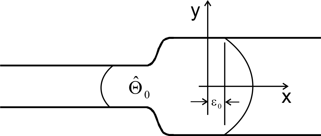
Figure 5. The domain $\hat{\Theta}_{0}$.

Let us now describe a method to extend the constructed flux $\mathscr{F}(\cdot,\cdot)$ carried in $\mathbf{O}_{i}$ into the domain $\Theta_{0}$ in a smooth manner. Let $\hat{\Theta}_{0}$ be an open subset of $\Theta$ with compact closure such that $\Theta_{0}\subset\hat{\Theta}_{0}\Subset\Theta$. Moreover, $\partial\hat{\Theta}_{0}$ is of class $C^{\infty}$ (see Figure 5).

Proposition 3.5.

There exists a vector field $\hat{\mathbf{w}}:\hat{\Theta}_{0}\times[0,T]\times\Omega\rightarrow\mathbb{R}^{2}$ in the form $\hat{\mathbf{w}}(\mathbf{x},t,\omega)=(\hat{\psi}_{y},-\hat{\psi}_{x})(\mathbf{x},t,\omega)$ for some stream function $\hat{\psi}$ such that

$$\nabla\cdot\hat{\mathbf{w}}=0\;\textrm{ in }\;\hat{\Theta}_{0}\times(0,T)\times\Omega$$

in the sense of distributions and

$$\hat{\mathbf{w}}(\mathbf{x},t,\omega) =0,\;t\in(0,T),\;\mathbf{x}=(x,y)\in\partial\hat{\Theta}_{0}\cap\partial\Theta,$$

$$\hat{\mathbf{w}}(\mathbf{x},t,\omega) =(w_{1}^{(i)}(y,t,\omega),0),\;t\in(0,T),\;\mathbf{x}=(x,y)\in\partial\hat{\Theta}_{0}\cap\mathbf{O}_{i},\;i=1,2,$$

for almost all $\omega\in\Omega$, in the sense of trace. Here $w^{(i)}_{1}(\cdot,\cdot,\cdot)$ denotes the solution of the heat equation constructed in $\mathbf{O}_{i}$. Moreover,

$$\hat{\mathbf{w}}\in\mathrm{L}^{2}(\Omega;\mathrm{L}^{2}(0,T;H^{2}(\hat{\Theta}_{0}))\cap C([0,T];H^{1}(\hat{\Theta}_{0})))$$

with $\partial_{t}\hat{\mathbf{w}}\in\mathrm{L}^{2}(\Omega;\mathrm{L}^{2}(0,T;\mathrm{L}^{2}(\hat{\Theta}_{0})))\subset\mathrm{L}^{2}(\Omega;\mathrm{L}^{2}(0,T;H^{-1}(\hat{\Theta}_{0}))).$

Proposition 3.5 can be deduced from the well-known method of extending the boundary data (with zero net flux) into the domain as a divergence-free vector field (Ladyzhenskaya [36]). Also we note that the regularity of the boundary data corresponds to that obtained in the solution of the heat equation and hence we have

$$\hat{\mathbf{w}}\big{|}_{\partial\hat{\Theta}_{0}}\in\mathrm{L}^{2}(\Omega;\mathrm{L}^{2}(0,T;H^{\frac{3}{2}+\varepsilon}(\partial\hat{\Theta}_{0}))\cap C([0,T];H^{\frac{1}{2}}(\partial\hat{\Theta}_{0})))$$

and

$$\partial_{t}\hat{\mathbf{w}}\big{|}_{\partial\hat{\Theta}_{0}}\in\mathrm{L}^{2}(\Omega;\mathrm{L}^{2}(0,T;H^{\varepsilon-\frac{1}{2}}(\partial\hat{\Theta}_{0}))),\;0\leq\varepsilon<\frac{1}{2}.$$

Let us use $\hat{\mathbf{w}}(\mathbf{x},t,\omega)$ in $\hat{\Theta}_{0}$ and $w_{1}^{(i)}(y,t,\omega)$ in $\mathbf{O}_{i}$, $i=1,2$ to construct the desired vector field $\mathbf{w}(\mathbf{x},t,\omega)$ in $\Theta$ (see Sritharan [62] for more details about the construction).

Let $\psi^{(i)}(y,t,\omega)$ be the stream function corresponding to the vector field

$$(w_{1}^{(i)}(y,t,\omega),0)=(\partial_{y}\psi^{(i)}(y,t,\omega),\partial_{x}\psi^{(i)}(y,t,\omega))$$

in $\mathbf{O}_{i}$. Let us set $\psi^{(i)}\big{|}_{y=0}=0$ on the lower wall of $\mathbf{O}_{i}$, hence on the upper wall of $\mathbf{O}_{i}$, we obtain

$$\mathscr{F}(t,\omega)=\int_{0}^{1}w_{1}(y,t,\omega)\/\mathrm{d}\/y=\int_{0}^{1}\frac{\partial}{\partial y}\psi^{(i)}(y,t,\omega)\/\mathrm{d}\/y=\psi^{(i)}(y,t,\omega)\Big{|}_{0}^{1}=\psi^{(i)}(1,t,\omega).$$

Also due to the flux condition, we have

$$\hat{\psi}\big{|}_{\partial\Theta_{2}\cap\partial\hat{\Theta}_{0}}=\mathscr{F}(t,\omega)\textrm{ and }\hat{\psi}\big{|}_{\partial\Theta_{1}\cap\partial\hat{\Theta}_{0}}=0.$$

Let us construct a $C^{\infty}$ function $\lambda(\cdot):\mathbb{R}\to(0,1)$ by mollifying a step function such that

$$\lambda(\xi)=\left\{\begin{array}[]{cl}0&\textrm{ for }\xi\leq 0,\\ 1&\textrm{ for }0<\varepsilon_{0}\leq\xi,\end{array}\right.$$

where $\varepsilon_{0}$ is a small number. Let us define

$$\psi(x,y,t,\omega)=(1-\lambda(x))\hat{\psi}(x,y,t,\omega)+\lambda(x)\psi^{(i)}(y,t,\omega)\textrm{ in }\hat{\Theta}_{0}\cap\mathbf{O}_{i},i=1,2,$$

for each $\omega\in\Omega$.

In this way we obtain a stream function which takes $\hat{\psi}(x,y,t,\omega)$ in $\Theta_{0}$ and smoothly become $\psi^{(i)}(y,t,\omega)$ in $\mathbf{O}_{i}$. On the lower wall $\partial\Theta_{1}$, we have

$$\psi(\mathbf{x},t,\omega)=\hat{\psi}(\mathbf{x},t,\omega)=\psi^{(i)}(y,t,\omega)=0$$

and on the upper wall $\partial\Theta_{2},$ we have

$$\psi(\mathbf{x},t,\omega)=\hat{\psi}(\mathbf{x},t,\omega)=\psi^{(i)}(y,t,\omega)=\mathscr{F}(t,\omega).$$

Hence we obtain the desired divergence free basic vector field as

$$\mathbf{w}(\mathbf{x},t,\omega)=(\partial_{y}\psi,-\partial_{x}\psi)(\mathbf{x},t,\omega).$$

A similar extension can be constructed for the scalar field $P(\mathbf{x},t,\omega)$ so that in $\Theta_{0}$,

$$P(\mathbf{x},t,\omega)\in\mathrm{L}^{2}(\Omega;\mathrm{L}^{2}(0,T;H^{1}(\Theta_{0})))$$

and becomes $-xf(t,\omega)$ smoothly in $\mathbf{O}_{i}$.

Let us now note some of the properties of the constructed basic vector field $\mathbf{w}(\mathbf{x},t,\omega)$:

• The flux condition, $\mathscr{F}(t,\omega)=\int_{\Gamma}\mathbf{w}(\mathbf{x},t,\omega)\cdot\mathbf{n}\/\mathrm{d}\/S$, where $\Gamma$ is any cross section of the channel.

• On the boundary, $\mathbf{x}\in\partial\Theta$, $\mathbf{w}(\mathbf{x},t,\omega)=0$, for all $t\in[0,T]$ and $\omega\in\Omega$.

• In the bounded region $\Theta_{0}$, the basic vector field $\mathbf{w}$ satisfies

  $$\mathbf{w}\in\mathrm{L}^{2}(\Omega;\mathrm{L}^{2}(0,T;H^{2}(\Theta_{0}))\cap C([0,T];H^{1}(\Theta_{0})))$$

  with $\mathbf{w}_{t}\in\mathrm{L}^{2}(\Omega;\mathrm{L}^{2}(0,T;H^{-1}(\Theta_{0}))).$ This gives, in $\Theta_{0}$

  $$\mathbf{w}_{t}-\nu\Delta\mathbf{w}+\mathbf{w}\cdot\nabla\mathbf{w}\in\mathrm{L}^{2}(\Omega;\mathrm{L}^{2}(0,T;H^{-1}(\Theta_{0}))).$$ (3.35)

  By the regularity of $\mathbf{w}$ in $\Theta_{0}$, we have

  $$\sup_{\mathbf{x}\in\Theta_{0}}|\mathbf{w}(\mathbf{x},\cdot,\omega)|=\beta_{10}(\cdot,\omega),\;\;\|\nabla\mathbf{w}(\mathbf{x},t,\omega)\|_{\mathrm{L}^{2}(0,T;\mathrm{L}^{2}(\Theta_{0}))}=\beta_{20}(\omega),$$ (3.36)

  where $\beta_{10}(\cdot,\cdot)\in\mathrm{L}^{2}(\Omega;\mathrm{L}^{2}(0,T))$ and $\beta_{20}(\cdot)\in\mathrm{L}^{2}(\Omega)$.

• In the infinite strips $\mathbf{O}_{i}$, (actually in $\mathbf{O}_{i}\backslash\hat{\Theta}_{0}$) $\mathbf{w}(x,y,t,\omega)$ becomes $w^{(i)}(y,t,\omega)$ and hence satisfies properties (i), (ii) above.

  Since, $w_{1}^{(i)}\in\mathrm{L}^{2}(\Omega;C^{1}([0,T];H^{1}(0,1))),$ we have

  $$\sup_{(\mathbf{x},t)\in\mathbf{O}_{i}\times(0,T)}|\mathbf{w}(\mathbf{x},t,\omega)|=\sup_{(y,t)\in(0,1)\times(0,T)}|w_{1}^{(i)}(y,t,\omega)|=\beta_{1i}(\omega),$$ (3.37)

  with $\beta_{1i}(\cdot)\in\mathrm{L}^{2}(\Omega).$

  Also, since $w_{1}^{(i)}\in\mathrm{L}^{2}(\Omega;\mathrm{L}^{2}(0,T;H^{2}(0,1)))$, we have

  $$\sup_{\mathbf{x}\in\mathbf{O}_{i}}|\nabla\mathbf{w}(\mathbf{x},\cdot,\omega)|=\sup_{y\in(0,1)}|\partial_{y}w_{1}^{(i)}(y,\cdot,\omega)|=\beta_{2i}(\cdot,\omega),$$ (3.38)

  with $\beta_{2i}(\cdot,\cdot)\in\mathrm{L}^{2}(\Omega;\mathrm{L}^{2}(0,T))$.

  In $\mathbf{O}_{i}$, $w_{1}^{(i)}$ is independent of the axial direction $x$, we have the constructed vector field $\mathbf{w}(\cdot,\cdot,\cdot)$ (for almost all time and almost all $\omega\in\Omega$) has infinite energy $\|\mathbf{w}\|_{\mathrm{L}^{2}(\Theta)}$ and infinite dissipation $\|\nabla\mathbf{w}\|_{\mathrm{L}^{2}(\Theta)}$ in $\Theta$, since

  $$\int_{0}^{\infty}\int_{0}^{1}|w_{1}^{(i)}(y,t,\omega)|^{2}\/\mathrm{d}\/y\/\mathrm{d}\/x=\infty\textrm{ and }\int_{0}^{\infty}\int_{0}^{1}|\partial_{y}w_{1}^{(i)}(y,t,\omega)|^{2}\/\mathrm{d}\/y\/\mathrm{d}\/x=\infty,$$

  $\mathbb{P}$ - a. s.

• Also note that in $\mathbf{O}_{i}$ (actually in $\mathbf{O}_{i}\backslash\hat{\Theta}_{0}$),

  $$\mathbf{w}_{t}-\nu\Delta\mathbf{w}+\mathbf{w}\cdot\nabla\mathbf{w}+\nabla P=0,$$

  for almost all $\omega\in\Omega.$

3.1. Connection between $\mathscr{F}$ and $\beta$.

Now let us establish certain connection between the norm of $\mathscr{F}$ and $\beta$ by using the properties of $\mathbf{w}$ in $\Theta_{0}$ and in the two outlets $\mathbf{O}_{1}$ and $\mathbf{O}_{2}$.

Proposition 3.6.

In $\Theta=\mathbf{O}_{1}\cup\mathbf{O}_{2}\cup\Theta_{0}$, the regularity properties of the basic vector field $\mathbf{w}$ implies that $\beta_{10}(\cdot,\cdot)\in\mathrm{L}^{2}(\Omega;\mathrm{L}^{2}(0,T));\;\beta_{11}(\cdot),\beta_{12}(\cdot)\in\mathrm{L}^{2}(\Omega)$ and $\beta_{20}(\cdot)\in\mathrm{L}^{2}(\Omega);\;\beta_{21}(\cdot,\cdot),\beta_{22}(\cdot,\cdot)\in\mathrm{L}^{2}(\Omega;\mathrm{L}^{2}(0,T)).$ Thus in $\Theta$, we have

$$\mathbb{E}\left[\int_{0}^{T}|\beta_{10}(t,\omega)|^{2}\/\mathrm{d}\/t+\left(\beta^{2}_{11}(\omega)+\beta^{2}_{12}(\omega)\right)T\right]\leq C(\pi,\nu,T)\|\mathscr{F}\|_{{}_{\mathrm{L}^{2}(\Omega;H^{1}(0,T))}}^{2}$$ (3.39)

and

$$\mathbb{E}\left[\beta^{2}_{20}(\omega)T+\int_{0}^{T}|\beta_{21}(t,\omega)|^{2}\/\mathrm{d}\/t+\int_{0}^{T}|\beta_{22}(t,\omega)|^{2}\/\mathrm{d}\/t\right]\leq C(\pi,\nu,T)\|\mathscr{F}\|_{{}_{\mathrm{L}^{2}(\Omega;H^{1}(0,T))}}^{2},$$ (3.40)

where $\beta$’s are defined in (3.36), (3.37) and (3.38).

Proof.

If we take $1+\varepsilon/2=\varsigma$ in the inequality (3), one can see that for $\rho<1$

$$\mathbb{E}\left(\int_{0}^{T}\|\mathscr{A}^{\varsigma}w_{1}(y,t,\omega)\|^{2}_{\mathrm{L}^{2}(0,1)}\/\mathrm{d}\/t\right)$$

$$\leq C_{1}(\pi,T,\nu)\|f(\cdot,\cdot)\|^{2}_{\mathrm{L}^{2}(\Omega;\mathrm{L}^{2}(0,T))}\sum_{n=0}^{\infty}(2n+1)^{4\varsigma-6}$$

$$\leq C_{1}(\pi,T,\nu)\left\|\sum_{p=0}^{\infty}\left[\mathscr{K}^{p}\frac{\partial}{\partial t}\mathscr{F}(t,\omega)\right]\right\|^{2}_{\mathrm{L}^{2}(\Omega;\mathrm{L}^{2}(0,T))}\sum_{n=0}^{\infty}(2n+1)^{4\varsigma-6}.$$ (3.41)

Now let us take the term $\left\|\sum_{p=0}^{\infty}\left[\mathscr{K}^{p}\frac{\partial}{\partial t}\mathscr{F}(t,\omega)\right]\right\|^{2}_{\mathrm{L}^{2}(\Omega;\mathrm{L}^{2}(0,T))}$ and use (3.21), (3.30) and Cauchy-Schwarz inequality to get

$$\left\|\sum_{p=0}^{\infty}\left[\mathscr{K}^{p}\frac{\partial}{\partial t}\mathscr{F}(t,\omega)\right]\right\|^{2}_{\mathrm{L}^{2}(\Omega;\mathrm{L}^{2}(0,T))}$$

$$=\mathbb{E}\left(\left\|\sum_{p=0}^{\infty}\left[\mathscr{K}^{p}\frac{\partial}{\partial t}\mathscr{F}(t,\omega)\right]\right\|^{2}_{\mathrm{L}^{2}(0,T)}\right)$$

$$=\mathbb{E}\left(\left<\sum_{p=0}^{\infty}\left[\mathscr{K}^{p}\frac{\partial}{\partial t}\mathscr{F}(t,\omega)\right],\sum_{m=0}^{\infty}\left[\mathscr{K}^{m}\frac{\partial}{\partial t}\mathscr{F}(t,\omega)\right]\right>_{\mathrm{L}^{2}(0,T)}\right)$$

$$\leq\mathbb{E}\left(\sum_{p=0}^{\infty}\sum_{m=0}^{\infty}\left|\left<\left[\mathscr{K}^{p}\frac{\partial}{\partial t}\mathscr{F}(t,\omega)\right],\left[\mathscr{K}^{m}\frac{\partial}{\partial t}\mathscr{F}(t,\omega)\right]\right>_{\mathrm{L}^{2}(0,T)}\right|\right)$$

$$\leq\mathbb{E}\left(\sum_{p=0}^{\infty}\sum_{m=0}^{\infty}\left\|\mathscr{K}^{p}\frac{\partial}{\partial t}\mathscr{F}(t,\omega)\right\|_{\mathrm{L}^{2}(0,T)}\left\|\mathscr{K}^{m}\frac{\partial}{\partial t}\mathscr{F}(t,\omega)\right\|_{\mathrm{L}^{2}(0,T)}\right)$$

$$<\mathbb{E}\left(\sum_{p=0}^{\infty}\sum_{m=0}^{\infty}\rho^{p}\left\|\frac{\partial}{\partial t}\mathscr{F}(t,\omega)\right\|_{\mathrm{L}^{2}(0,T)}\rho^{m}\left\|\frac{\partial}{\partial t}\mathscr{F}(t,\omega)\right\|_{\mathrm{L}^{2}(0,T)}\right)$$

$$=\mathbb{E}\left(\sum_{p=0}^{\infty}\rho^{p}\sum_{m=0}^{\infty}\rho^{m}\left\|\frac{\partial}{\partial t}\mathscr{F}(t,\omega)\right\|_{\mathrm{L}^{2}(0,T)}^{2}\right)=\mathbb{E}\left(\left(\frac{1}{1-\rho}\right)^{2}\left\|\frac{\partial\mathscr{F}}{\partial t}\right\|_{\mathrm{L}^{2}(0,T)}^{2}\right)$$

$$=\left(\frac{1}{1-\rho}\right)^{2}\left\|\frac{\partial\mathscr{F}}{\partial t}\right\|_{\mathrm{L}^{2}(\Omega;\mathrm{L}^{2}(0,T))}^{2}$$

Hence the inequality (3.1) becomes

$$\mathbb{E}\left(\int_{0}^{T}\|\mathscr{A}^{\varsigma}w_{1}(y,t,\omega)\|^{2}_{\mathrm{L}^{2}(0,1)}\/\mathrm{d}\/t\right)$$

$$\leq C_{1}(\pi,T,\nu)\left(\frac{1}{1-\rho}\right)^{2}\left\|\frac{\partial\mathscr{F}}{\partial t}\right\|_{\mathrm{L}^{2}(\Omega;\mathrm{L}^{2}(0,T))}^{2}\sum_{n=0}^{\infty}(2n+1)^{4\varsigma-6}.$$

The series $\sum_{n=0}^{\infty}(2n+1)^{4\varsigma-6}$ is convergent for $0\leq\varsigma<\frac{5}{4}$. Hence for $0\leq\varsigma<\frac{5}{4}$ and for $\rho<1$, we get

$$\mathbb{E}\left(\int_{0}^{T}\|\mathscr{A}^{\varsigma}w_{1}(y,t,\omega)\|^{2}_{\mathrm{L}^{2}(0,1)}\/\mathrm{d}\/t\right) \leq C_{2}(\pi,T,\nu)\sum_{n=0}^{\infty}(2n+1)^{4\varsigma-6}\left\|\frac{\partial\mathscr{F}}{\partial t}\right\|_{\mathrm{L}^{2}(\Omega;\mathrm{L}^{2}(0,T))}^{2}$$

$$\leq C_{3}\|\mathscr{F}(t)\|^{2}_{{}_{\mathrm{L}^{2}(\Omega;H^{1}(0,T))}}.$$ (3.42)

By using the estimates (3.37) and (3.38), by taking $\varsigma=0,\frac{1}{2}$ in (3.1), one can easily see that

$$\mathbb{E}\left[\int_{0}^{T}|\beta_{21}(t,\omega)|^{2}\/\mathrm{d}\/t+\int_{0}^{T}|\beta_{22}(t,\omega)|^{2}\/\mathrm{d}\/t\right]$$

$$=\mathbb{E}\left[\int_{0}^{T}\sup_{y\in(0,1)}|\partial_{y}w_{1}^{(1)}(y,t,\omega)|^{2}\/\mathrm{d}\/t+\int_{0}^{T}\sup_{y\in(0,1)}|\partial_{y}w_{1}^{(2)}(y,t,\omega)|^{2}\/\mathrm{d}\/t\right]$$

$$\leq C\|\mathscr{F}(t)\|^{2}_{{}_{\mathrm{L}^{2}(\Omega;H^{1}(0,T))}}$$

and

$$\mathbb{E}\left[(\beta^{2}_{11}(\omega)+\beta^{2}_{12}(\omega))\right]T$$

$$=\mathbb{E}\left[\int_{0}^{T}\sup_{(y,t)\in(0,1)\times(0,T)}|w_{1}^{(1)}(y,t,\omega)|^{2}\/\mathrm{d}\/t+\int_{0}^{T}\sup_{(y,t)\in(0,1)\times(0,T)}|w_{1}^{(2)}(y,t,\omega)|^{2}\/\mathrm{d}\/t\right]$$

$$\leq C\|\mathscr{F}\|^{2}_{{}_{\mathrm{L}^{2}(\Omega;H^{1}(0,T))}}$$

in $\mathbf{O}_{i}$.

Since $\Theta_{0}$ is bounded, by using property (iii) of the basic vector field and we extended the constructed flux $\mathscr{F}(t,\omega)=\int_{\Gamma}\mathbf{w}\cdot\mathbf{n}\/\mathrm{d}\/S$ carried in $\mathbf{O}_{i}$ into the domain $\Theta_{0}$ in a smooth manner, it can be easily shown that

$$\mathbb{E}\left[\beta^{2}_{20}(\omega)\right]T\leq C\|\mathscr{F}\|^{2}_{{}_{\mathrm{L}^{2}(\Omega;H^{1}(0,T))}}\textrm{ and }\mathbb{E}\left[\int_{0}^{T}|\beta_{10}(t,\omega)|^{2}\/\mathrm{d}\/t\right]\leq C\|\mathscr{F}\|^{2}_{{}_{\mathrm{L}^{2}(\Omega;H^{1}(0,T))}}.$$

Hence, we have the relation (3.39) and (3.40) in $\Theta$. ∎

Remark 3.7.

From (3.38), we have

$$\sup_{\mathbf{x}\in\mathbf{O}_{i}}|\nabla\mathbf{w}(\mathbf{x},\cdot,\omega)|=\beta_{2i}(\cdot,\omega)\in\mathrm{L}^{2}(\Omega;\mathrm{L}^{2}(0,T)).$$

For $i=1,2$, we can always get an upper bound for $\beta_{2i}(t,\omega)$ for all $t\in[0,T]$ and almost all $\omega\in\Omega$. By using (3.9) and Young’s inequality for convolution of two functions, we obtain

$$\sup_{0\leq t\leq T}\sup_{\mathbf{x}\in\mathbf{O}_{2}}|\nabla\mathbf{w}(\mathbf{x},t,\omega)|^{2}$$

$$=\sup_{0\leq t\leq T}\sup_{y\in(0,1)}\left|\frac{\partial}{\partial y}\left(\frac{4}{\pi}\sum_{n=0}^{\infty}\left\{\int_{0}^{t}f(s,\omega)\frac{1}{2n+1}e^{-\nu(2n+1)^{2}\pi^{2}(t-s)}\/\mathrm{d}\/s\right\}\right.\right.$$

$$\quad\sin(2n+1)\pi y\Big{)}\Big{|}^{2}$$

$$\leq\sup_{0\leq t\leq T}4\pi\sum_{n=0}^{\infty}\int_{0}^{t}|f(s,\omega)|^{2}e^{-2\nu(2n+1)^{2}\pi^{2}(t-s)}\/\mathrm{d}\/s$$

$$\leq 4\pi\sup_{0\leq t\leq T}\sum_{n=0}^{\infty}\left(\int_{0}^{t}|f(s,\omega)|^{2}\/\mathrm{d}\/s\right)\left(\int_{0}^{t}e^{-2\nu(2n+1)^{2}\pi^{2}t}\/\mathrm{d}\/s\right)$$

$$\leq\frac{2}{\pi\nu}\sup_{0\leq t\leq T}\sum_{n=0}^{\infty}\frac{1}{(2n+1)^{2}}\int_{0}^{t}|f(s,\omega)|^{2}\/\mathrm{d}\/s$$

$$\leq\frac{\pi}{4\nu}\|f(t,\omega)\|^{2}_{\mathrm{L}^{2}(0,T)}=\eta_{22}^{2}(\omega),$$ (3.43)

where $\eta_{22}(\omega)\in\mathrm{L^{2}}(\Omega)$, since $f\in\mathrm{L}^{2}(\Omega;C([0,T]))\subset\mathrm{L}^{2}(\Omega;\mathrm{L}^{2}(0,T))$.

Hence, we get $\sup_{t\in[0,T]}\beta_{2i}^{2}(t,\omega)\leq\eta^{2}_{2i}(\omega)\textrm{ for }i=1,2$, $\mathbb{P}$-a. s.

4. The Linear and Multilinear Operators

In this section we define the Stokes operator, the inertia operator and the other operators relevant to our analysis. Most of the results obtained in this section has been taken from [62] given here for completeness.

4.1. The Stokes Operator

Let us first define the Stokes operator for the two-dimensional admissible channel domain and analyze its properties. Let us denote by $a(\cdot,\cdot)$ the symmetric bilinear form

$$a(\mathbf{u},\mathbf{v})=\int_{\Theta}\nabla\mathbf{u}\cdot\nabla\mathbf{v}\/\mathrm{d}\/\mathbf{x}.$$ (4.1)

Let us now define the Stokes operator $A$ and its domain $D(A)$ in the following way. Given $\mathbf{u}\in\mathbf{V}$, if there exists an element $\mathbf{g}\in\mathbf{H}$ such that

$$a(\mathbf{u},\mathbf{v})=(\mathbf{g},\mathbf{v})_{\mathbf{H}},\ \;\forall\;\mathbf{v}\in\mathbf{V},$$

then we say $\mathbf{u}\in D(A)$ and $A\mathbf{u}=g.$ By Poincaré inequality $\|\mathbf{u}\|_{\mathrm{L}^{2}(\Theta)}\leq C\|\nabla\mathbf{u}\|_{\mathrm{L}^{2}(\Theta)}$ holds for the admissible channel domains, we obtain the coerciveness ($\mathbf{V}$-elliptic) property as,

$$a(\mathbf{u},\mathbf{u})=\|\nabla\mathbf{u}\|^{2}_{\mathrm{L}^{2}(\Theta)}\geq C\|\mathbf{u}\|^{2},\;\forall\;\mathbf{u}\in\mathbf{V}.$$

Since the form $a(\cdot,\cdot)$ is symmetric, continuous, and positive definite, we have the following standard results obtained in [66].

Proposition 4.1.

There exists a self-adjoint, regularly accretive onto map $\tilde{A}\in\mathscr{L}(D(\tilde{A});\mathbf{H})$ such that

$$a(\mathbf{u},\mathbf{v})=(\tilde{A}\mathbf{u},\mathbf{v})_{\mathbf{H}},\;\forall\;\mathbf{u}\in D(A),\;\forall\;\mathbf{v}\in\mathbf{V},$$

with $D(\tilde{A})\subset\mathbf{V}$ dense. Moreover, it is possible to extend this operator as an isomorphic onto map $\hat{A}\in\mathscr{L}(\mathbf{V},\mathbf{V}^{\prime})$ such that

$$a(\mathbf{u},\mathbf{v})=(\hat{A}\mathbf{u},\mathbf{v})_{\mathbf{V}\times\mathbf{V}^{\prime}},\;\forall\;\mathbf{u},\mathbf{v}\in\mathbf{V}.$$

The operators $\tilde{A}$ and $\hat{A}$ are different Friedrich’s extensions of the classical Stokes operator. In the remainder of the paper, both of these operators will be denoted by $A$. It follows from a general theorem of Lions [42] that $\mathbf{V}=D(A^{1/2})$. Let the orthogonal Helmhotz-Hodge projection $P_{\mathbf{H}}:\mathrm{L}^{2}(\Theta,\mathbb{R}^{2})\rightarrow\mathrm{H}$ and $A\mathbf{u}=-P_{\mathbf{H}}\Delta\mathbf{u}\;\forall\;\mathbf{u}\in D(A).$

Let us now state a regularity theorem. This give us an explicit representation of $D(A)$.

Lemma 4.2.

Let $\Theta$ be an admissible channel domain. Then, for a given $\mathbf{g}\in R(A)=\mathbf{H}$, the Stokes problem of finding $(\mathbf{u},p):\Theta\rightarrow\mathbb{R}^{2}\times\mathbb{R}$ such that

$$-\Delta\mathbf{u}+\nabla p =\mathbf{g}\;\textrm{ in }\;\Theta$$

$$\nabla\cdot\mathbf{u} =0\;\textrm{ in }\;\Theta$$

$$\mathbf{u}\big{|}_{\partial\Theta} =0,\;\;\mathbf{u}\rightarrow 0\;\textrm{ as }\;|x|\rightarrow\infty\;\textrm{ in }\;\mathbf{O}_{i}\textrm{ and }$$

$$\int_{\Gamma}\mathbf{u}\cdot\mathbf{n}\/\mathrm{d}\/S =0,$$

has a unique solution $\mathbf{u}$ that satisfies $\mathbf{u}\in D(A)=H^{2}(\Theta)\cap\mathbf{V}.$ Moreover, if we define the graph norm

$$\|\mathbf{u}\|_{D(A)}=\|\mathbf{u}\|_{\mathrm{L}^{2}(\Theta)}+\|A\mathbf{u}\|_{\mathrm{L}^{2}(\Theta)},\;\forall\;\mathbf{u}\in D(A),$$

then there exists $C>0$ such that, $C\|\mathbf{u}\|_{H^{2}(\Theta)}\leq\|\mathbf{u}\|_{D(A)}\leq\|\mathbf{u}\|_{H^{2}(\Theta)}.$

Proof.

For proof see Theorem 3, section 4 of [62]. ∎

4.2. The Bilinear Operator (Inertia Term)

Let us now define the trilinear form and the bilinear operator and their properties. The trilinear form is given by,

$$b(\mathbf{u},\mathbf{v},\phi)=\sum_{i,j=1}^{2}\int_{\Theta}\mathbf{u}_{i}\frac{\partial\mathbf{v}_{j}}{\partial x_{i}}\phi_{j}\/\mathrm{d}\/\mathbf{x}.$$ (4.2)

It is well known that trilinear form $b(\cdot,\cdot,\cdot):\mathbf{V}\times\mathbf{V}\times\mathbf{V}\rightarrow\mathbb{R}$ is continuous and for all $\mathbf{u},\mathbf{v},\phi\in\mathbf{V}$ we have

$$b(\mathbf{u},\mathbf{v},\phi)=-b(\mathbf{u},\phi,\mathbf{v})\;\textrm{ and }\;b(\mathbf{u},\mathbf{v},\mathbf{v})=0.$$

The following lemma is standard.

Lemma 4.3.

[62] There exist continuous bilinear operators, $B(\cdot,\cdot):\mathbf{V}\times\mathbf{V}\rightarrow\mathbf{V}^{\prime}$ and $B^{*}(\cdot,\cdot):\mathbf{V}\times\mathbf{V}\rightarrow\mathbf{V}^{\prime}$ such that

$$b(\mathbf{u},\mathbf{v},\phi)=(B(\mathbf{u},\mathbf{v}),\phi)_{\mathbf{V}^{\prime}\times\mathbf{V}}=(B^{*}(\mathbf{v},\phi),\mathbf{u})_{\mathbf{V}^{\prime}\times\mathbf{V}},\;\forall\;\mathbf{u},\mathbf{v},\phi\in\mathbf{V}.$$ (4.3)

Moreover,

$$\|B(\mathbf{u},\mathbf{v})\|_{\mathbf{V}^{\prime}} \leq C\|\mathbf{u}\|^{1/2}_{\mathrm{L}^{2}(\Theta)}\|\nabla\mathbf{u}\|^{1/2}_{\mathrm{L}^{2}(\Theta)}\|\mathbf{v}\|^{1/2}_{\mathrm{L}^{2}(\Theta)}\|\nabla\mathbf{v}\|^{1/2}_{\mathrm{L}^{2}(\Theta)},$$ (4.4)

$$\|B^{*}(\mathbf{v},\phi)\|_{\mathbf{V}^{\prime}} \leq C\|\nabla\mathbf{v}\|_{\mathrm{L}^{2}(\Theta)}\|\phi\|^{1/2}_{\mathrm{L}^{(}\Theta)}\|\nabla\phi\|_{\mathrm{L}^{2}(\Theta)}^{1/2}$$ (4.5)

and

$$B^{*}(\mathbf{v},\phi)=-B^{*}(\phi,\mathbf{v}),\quad\forall\;\phi,\mathbf{v}\in\mathbf{V}.$$ (4.6)

Now we will provide a general setting for estimating the terms $b(\mathbf{w},\cdot,\cdot)$ and $b(\cdot,\mathbf{w},\cdot)$, where $\mathbf{w}$ is the basic vector field constructed in section $3$.

Lemma 4.4.

The trilinear form $b(\mathbf{w},\cdot,\cdot):\mathbf{V}\times\mathbf{V}\rightarrow\mathbb{R}$ is continuous and satisfies,

$$(i)\;\;b(\mathbf{w},\mathbf{u},\mathbf{v}) =-b(\mathbf{w},\mathbf{v},\mathbf{u}),\;\forall\;\mathbf{u},\mathbf{v}\in\mathbf{V}\;\textrm{ and }$$ (4.7)

$$(ii)\;\;b(\mathbf{w},\mathbf{u},\mathbf{u}) =0,\;\forall\;\mathbf{u}\in\mathbf{V}.$$ (4.8)

Proof.

For proof see Lemma 4, section 4 of [62]. ∎

Lemma 4.5.

The form $b(\cdot,\mathbf{w},\cdot):\mathbf{V}\times\mathbf{V}\rightarrow\mathbb{R}$ is continuous.

Proof.

For proof see Lemma 5, section 4 of [62]. ∎

Lemma 4.6.

There exists a continuous linear operator $B_{1}(\mathbf{w})\in\mathscr{L}(\mathbf{V};\mathbf{V}^{\prime})$ such that

$$(i)\;\;b(\mathbf{w},\mathbf{u},\mathbf{v})=(B_{1}(\mathbf{w})\mathbf{u},\mathbf{v})_{\mathbf{V}^{\prime}\times\mathbf{V}},\;\forall\;\mathbf{u},\mathbf{v}\in\mathbf{V}.$$

Moreover,

$$(ii)\;\;(B_{1}(\mathbf{w})\mathbf{u},\mathbf{v})_{\mathbf{V}^{\prime}\times\mathbf{V}}=-(B_{1}(\mathbf{w})\mathbf{v},\mathbf{u})_{\mathbf{V}^{\prime}\times\mathbf{V}},\;\forall\;\mathbf{u},\mathbf{v}\in\mathbf{V}.$$

Proof.

For proof see Lemma 6, section 4 of [62]. ∎

Lemma 4.7.

There exists a continuous linear operators $B_{2}(\mathbf{w})\in\mathscr{L}(\mathbf{V};\mathbf{V}^{\prime})$ and $B_{2}(\mathbf{w})^{*}\in\mathscr{L}(\mathbf{V}^{\prime};\mathbf{V})$ such that

$$(i)\;\;(B_{2}(\mathbf{w})\mathbf{u},\mathbf{v})_{\mathbf{V}^{\prime}\times\mathbf{V}}=(\mathbf{u},B_{2}(\mathbf{w})^{*}\mathbf{v})_{\mathbf{V}^{\prime}\times\mathbf{V}}=b(\mathbf{u},\mathbf{w},\mathbf{v}),\;\forall\;\mathbf{u},\mathbf{v}\in\mathbf{V}.$$

Moreover,

$$(ii)\;\;\|B_{2}(\mathbf{w})\|_{\mathscr{L}(\mathbf{V};\mathbf{V^{\prime}})}=\|B_{2}(\mathbf{w})^{*}\|_{\mathscr{L}(\mathbf{V^{\prime}};\mathbf{V})}\leq\beta_{20}(\omega)+\sum_{i=1}^{2}\beta_{2i}(t,\omega).$$

Proof.

For proof see Lemma 7, section 4 of [62]. ∎

By taking the Helmhotz-Hodge projection $P_{\mathbf{H}}$, we get

$$B(\mathbf{u},\mathbf{v})=P_{\mathbf{H}}(\mathbf{u}\cdot\nabla\mathbf{v}),B_{1}(\mathbf{w})\mathbf{v}=P_{\mathbf{H}}(\mathbf{w}\cdot\nabla\mathbf{v}),B_{2}(\mathbf{w})\mathbf{v}=P_{\mathbf{H}}(\mathbf{v}\cdot\nabla\mathbf{w}),\;\forall\;\mathbf{u},\mathbf{v}\in\mathbf{V}.$$

Remark 4.8.

For the notational convenience from now onwards we use the symbols $\overline{\beta}_{10}(t)=\mathbb{E}[\beta_{10}(t,\omega)],$ $\overline{\beta}_{1j}=\mathbb{E}[\beta_{1j}(\omega)]$ for $j=1,2$, $\overline{\beta}^{2}_{20}=\mathbb{E}[\beta^{2}_{20}(\omega)]$ and $\overline{\beta}_{2j}(t)=\mathbb{E}[\beta_{2j}(t,\omega)]$ for $j=1,2$.

5. Construction of the Perturbed Vector Field

Let us now consider the system (2.2)-(2.6) and introduce the following change of variables:

$$\mathbf{u}(\mathbf{x},t,\omega)=\mathbf{v}(\mathbf{x},t,\omega)+\mathbf{w}(\mathbf{x},t,\omega)\textrm{ and }p(\mathbf{x},t,\omega)=q(\mathbf{x},t,\omega)+P(\mathbf{x},t,\omega),$$

where $\mathbf{w}(\cdot,\cdot,\cdot)$ is the basic vector field. The regularity properties of this basic vector field imply the following properties on $\beta_{1j}$ and $\beta_{2j},$ for $j=0,1,2$:

$$\beta_{11}(\omega),\beta_{12}(\omega),\beta_{20}(\omega)\in\mathrm{L}^{2}(\Omega)\textrm{ and }\beta_{10}(t,\omega),\beta_{21}(t,\omega),\beta_{22}(t,\omega)\in\mathrm{L}^{2}(\Omega;\mathrm{L}^{2}(0,T)).$$

Our problem is to find

$$(\mathbf{v},q):\Theta\times[0,T]\times\Omega\rightarrow\mathbb{R}^{2}\times\mathbb{R}$$

such that

$$\mathbf{v}_{t}+\mathbf{v}\cdot\nabla\mathbf{v}+\mathbf{v}\cdot\nabla\mathbf{w}+\mathbf{w}\cdot\nabla\mathbf{v} =-\nabla q+\nu\Delta\mathbf{v}+\mathbf{f}_{\mathbf{w}}+\dot{\mathscr{G}}(\mathbf{x},t)$$

$$\quad\textrm{ in }\Theta\times(0,T)\times\Omega,$$ (5.1)

$$\nabla\cdot\mathbf{v} =0\textrm{ in }\Theta\times(0,T)\times\Omega,$$ (5.2)

$$\mathbf{v}\big{|}_{\partial\Theta\times[0,T]\times\Omega} =0,$$ (5.3)

$$\mathbf{v} \rightarrow 0\textrm{ as }|\mathbf{x}|\rightarrow\infty\textrm{ in }\mathbf{O}_{i},i=1,2,$$ (5.4)

$$\mathbf{v}(\mathbf{x},0,\omega) =0,(\mathbf{x},\omega)\in\Theta\times\Omega\quad\textrm{ and }$$ (5.5)

$$\int_{\Gamma}\mathbf{v}\cdot\mathbf{n}\/\mathrm{d}\/S =0,$$ (5.6)

where

$$\mathbf{f}_{\mathbf{w}}=\nu\Delta\mathbf{w}-\mathbf{w}\cdot\nabla\mathbf{w}-\mathbf{w}_{t}-\nabla P.$$ (5.7)

From the construction of the basic vector field it is clear that the supp$\{\mathbf{f}_{\mathbf{w}}\}\Subset\Theta$. Also one can notice that $\mathbf{f}_{\mathbf{w}}\equiv 0$ for $\mathbf{O}_{i}\backslash\hat{\Theta}_{0}$. Moreover, form the estimate

$$\mathbf{w}_{t}-\nu\Delta\mathbf{w}+\mathbf{w}\cdot\nabla\mathbf{w}\in\mathrm{L}^{2}\left(\Omega;\mathrm{L}^{2}(0,T;H^{-1}(\Theta_{0}))\right),$$

we have $\mathbf{f}_{\mathbf{w}}\in\mathrm{L}^{2}\left(\Omega;\mathrm{L}^{2}(0,T;\mathbf{V}^{\prime})\right).$ A-priori estimates for the solution can be obtained by assuming smoothness of $\mathbf{v}$ and sufficient decay at infinity.

Let us now take the Helmhotz-Hodge projection on the equation (5) and using the fact that $(\nabla q,\mathbf{v})=0$, $\forall\;\mathbf{v}\in\mathbf{H}$, one can reduce the equation (5) to

$$\/\mathrm{d}\/\mathbf{v} =(F(\mathbf{v}(t))+P_{\mathbf{H}}\mathbf{f}_{\mathbf{w}}(t))\/\mathrm{d}\/t+g(t)\/\mathrm{d}\/W(t),$$ (5.8)

$$\textrm{where }\;\;F(\mathbf{v}(t)) =-\nu A\mathbf{v}-B(\mathbf{v},\mathbf{v})-B_{1}(\mathbf{w})\mathbf{v}-B_{2}(\mathbf{w})\mathbf{v}$$

$$A\mathbf{v} =-P_{\mathbf{H}}\Delta\mathbf{v}$$

$$B(\mathbf{u},\mathbf{v}) =P_{\mathbf{H}}(\mathbf{u}\cdot\nabla\mathbf{v})$$

$$B_{1}(\mathbf{w})\mathbf{v} =P_{\mathbf{H}}(\mathbf{w}\cdot\nabla\mathbf{v})$$

$$B_{2}(\mathbf{w})\mathbf{v} =P_{\mathbf{H}}(\mathbf{v}\cdot\nabla\mathbf{w}).$$

See Appendix of Mikulevicius and Rozovskii [49] for more details about the properties of the projection operator.

Let the noise process be represented as a series $\/\mathrm{d}\/\mathscr{G}_{k}=\sum_{k}g_{k}(\mathbf{x},t)\/\mathrm{d}\/W_{k}(t,\omega)$, where $g=(g_{1},g_{2},\cdots)$ is and $\ell^{2}$- valued function and $W_{k}$ are mutually independent standard one dimensional Brownian motions. The stochastic term $g\/\mathrm{d}\/W$ is thus an $\mathbf{H}$ - valued Wiener process with a trace-class covariance operator denoted by $g^{*}g=g^{*}g(t)$ given by

$$\left(g^{*}g(t)u,v\right) =\sum_{k}\left(g_{k}(t),u\right)\left(g_{k}(t),v\right),$$

$$\textrm{Tr}(g^{*}g(t)) =\sum_{k}\left|g_{k}(t)\right|^{2}<\infty.$$

This means that the mapping

$$v\rightarrow\int_{0}^{T}\left(g(t)\/\mathrm{d}\/W(t),v\right):=\sum_{k}\int_{0}^{T}\left(g_{k}(t),v\right)\/\mathrm{d}\/W_{k}(t)$$

is a continuous linear functional on $\mathbf{H}$ with probability $1$ and the noise is the formal time-derivative of the process $P_{\mathbf{H}}\mathscr{G}(t)=\int_{0}^{t}g(t)\/\mathrm{d}\/W(t)$. A multiplicative noise of the form $g(\mathbf{u}(\mathbf{x},t))\/\mathrm{d}\/W(t)$, where $g(\mathbf{u}(\mathbf{x},t))$ is a continuous operator from $\mathbf{V}$ into $\mathrm{L}^{2}(0,T;\ell^{2}(\mathbf{H}))$, can also be considered as the random forcing. Here $\dot{\mathscr{G}}(\cdot)$ is formally written and it is the time-derivative of $\int_{0}^{\cdot}g(s)\/\mathrm{d}\/W(s)$. We have $\int_{0}^{\cdot}g(s)\/\mathrm{d}\/W(s)\in\mathrm{L}^{2}(\Omega;C([0,T];\mathbf{H}))$ implies its time-derivative $\dot{\mathscr{G}}(\cdot)$ satisfies $\dot{\mathscr{G}}(\cdot)\in\mathrm{L}^{2}(\Omega;\mathrm{W}^{-1,\infty}(0,T;\mathbf{H})),$ since $\partial_{t}$ is linear continuous from $C([0,T];\mathbf{H})$ into $W^{-1,\infty}(0,T;\mathbf{H})$.

6. A-Priori Estimates for the Perturbed Vector Field

Let $\mathbf{H}_{n}=span\{e_{1},e_{2},\cdots,e_{n}\},$ where $\{e_{j}\}$ is any fixed orthonormal basis in $\mathbf{H}$ with $e_{j}\in D(A)$. Let $P_{n}$ denote the orthogonal projection of $\mathbf{H}$ into $\mathbf{H}_{n}$. Define $\mathbf{v}^{n}=P_{n}\mathbf{v}$. Let us define $\mathbf{v}^{n}$ as the solution of the following stochastic differential equation in the variational form such that for each $v\in\mathbf{H}_{n}$,

$$\/\mathrm{d}\/(\mathbf{v}^{n}(t),v) =(F(\mathbf{v}^{n}(t)),v)\/\mathrm{d}\/t+(P_{\mathbf{H}}\mathbf{f}_{\mathbf{w}}(t),v)\/\mathrm{d}\/t+\sum_{k}(g_{k}(t),v)\/\mathrm{d}\/W_{k}(t),$$ (6.1)

$$\mathbf{v}^{n}(0) =P_{n}\mathbf{v}(0)\;=\;0,$$

where $F(\mathbf{v})=-\nu A\mathbf{v}-B(\mathbf{v},\mathbf{v})-B_{1}(\mathbf{w})\mathbf{v}-B_{2}(\mathbf{w})\mathbf{v}.$

It can be shown that for all $n\geq 1$, there exists an adapted process $\mathbf{v}^{n}\in C([0,T];\mathbf{H}_{n})$ a. s. such that $\mathbf{v}^{n}$ satisfies (6.1). For proof see corollary 2.1 of Albeverio, Brzeźniak, Wu [1], page 128 of Brzeźniak, Hausenblas, Zhu [13], Lemma 3.1 of Capiński and Peszat [15], Proposition 3.2 of Manna, Menaldi and Sritharan [45], Theorem 3.1.1 of Prévôt and Röckner [54].

Theorem 6.1.

Let $\Theta$ be an admissible channel domain. Under the above mathematical setting, let $\mathbf{v}^{n}(t)$ be an adapted process in $C([0,T];\mathbf{H}_{n})$ which solves the stochastic ODE (6.1). Then we have the following a-priori estimates: For $\delta>0$

$$\mathbb{E}\left|\mathbf{v}^{n}(\cdot,t)\right|^{2}e^{-\delta t}+\nu\mathbb{E}\left(\int_{0}^{t}\|\mathbf{v}^{n}(\cdot,s)\|^{2}e^{-\delta s}\/\mathrm{d}\/s\right)$$

$$\qquad\quad\leq C_{1}\left(T,\nu,\|\mathscr{F}\|_{{}_{\mathrm{L}^{2}(\Omega;H^{1}(0,T))}},\delta,\int_{0}^{T}\mathop{\mathrm{Tr}}(g^{*}g)(t)e^{-\delta t}\/\mathrm{d}\/t\right)$$ (6.2)

and

$$\mathbb{E}\left[\sup_{0\leq t\leq T}\left|\mathbf{v}^{n}(\cdot,t)\right|^{2}e^{-\delta t}\right]+2\nu\mathbb{E}\left(\int_{0}^{T}\|\mathbf{v}^{n}(\cdot,t)\|^{2}e^{-\delta t}\/\mathrm{d}\/s\right)$$

$$\quad\quad\leq C_{2}\left(T,\nu,\|\mathscr{F}\|_{{}_{\mathrm{L}^{2}(\Omega;H^{1}(0,T))}},\delta,\int_{0}^{T}\mathop{\mathrm{Tr}}(g^{*}g)(t)e^{-\delta t}\/\mathrm{d}\/t\right).$$ (6.3)

Proof.

Let us consider the function $e^{-\delta t}|x|^{2}$ and apply Itô’s lemma (see Theorem 1, page 155 Gyöngy and Krylov [26], Metivier [48]) to the process $\mathbf{v}^{n}(t)$, for any $\delta>0$

$$\/\mathrm{d}\/\left[e^{-\delta t}|\mathbf{v}^{n}|^{2}\right]=-\delta e^{-\delta t}|\mathbf{v}^{n}|^{2}\/\mathrm{d}\/t-2\left[b(\mathbf{v}^{n},\mathbf{v}^{n},\mathbf{v}^{n})+b(\mathbf{v}^{n},\mathbf{w},\mathbf{v}^{n})\right.$$

$$\qquad\qquad\qquad\left.+b(\mathbf{w},\mathbf{v}^{n},\mathbf{v}^{n})+\nu(\Delta\mathbf{v}^{n},\mathbf{v}^{n})\right]e^{-\delta t}\/\mathrm{d}\/t+\left[(P_{\mathbf{H}}\mathbf{f}_{\mathbf{w}},\mathbf{v}^{n})\right]e^{-\delta t}\/\mathrm{d}\/t$$

$$\qquad\qquad\qquad+2\sum_{k}(g_{k}(t),\mathbf{v}^{n})e^{-\delta t}\/\mathrm{d}\/W_{k}(t)+e^{-\delta t}\mathrm{Tr}(g^{*}g)(t)\/\mathrm{d}\/t.$$ (6.4)

By applying the properties of the trilinear form, $(\Delta\mathbf{v}^{n},\mathbf{v}^{n})=-\|\mathbf{v}^{n}\|^{2}$ and $2|(P_{\mathbf{H}}\mathbf{f}_{\mathbf{w}},\mathbf{v}^{n})|\leq\delta|\mathbf{v}^{n}|^{2}+\frac{1}{\delta}|\mathbf{f}_{\mathbf{w}}|^{2}$ in (6), we get

$$\/\mathrm{d}\/\left[[e^{-\delta t}|\mathbf{v}^{n}|^{2}\right]+2\nu\|\mathbf{v}^{n}\|^{2}e^{-\delta t}\/\mathrm{d}\/t\leq-2b(\mathbf{v}^{n},\mathbf{w},\mathbf{v}^{n})e^{-\delta t}\/\mathrm{d}\/t+\frac{1}{\delta}|\mathbf{f}_{\mathbf{w}}|^{2}e^{-\delta t}\/\mathrm{d}\/t$$

$$\qquad\qquad\qquad\qquad+e^{-\delta t}\mathrm{Tr}(g^{*}g)(t)\/\mathrm{d}\/t+2\sum_{k}(g_{k}(t),\mathbf{v}^{n})e^{-\delta t}\/\mathrm{d}\/W_{k}(t).$$ (6.5)

Let $\mathcal{G}$ be the $\sigma$-algebra generated by $\mathbf{v}^{n}$ in the probability space $(\Omega;\mathcal{F},\mathcal{F}_{t},\mathbb{P})$. Since we have assumed that the external random forcing and the random flux are mutually independent processes, the constructed vector field $\mathbf{w}$ is independent of $\mathcal{G}$.

Let us define the stopping time $\tau_{N}$ by

$$\tau_{N}=\inf\left\{t:|\mathbf{v}^{n}(t)|^{2}+\int_{0}^{t}\|\mathbf{v}^{n}(s)\|^{2}\/\mathrm{d}\/s>N\right\}.$$

Note that $\tau_{N}$ is adapted to $\mathcal{G}$ and $\mathbf{w}$ is independent of $\mathcal{G}$.

Now let us integrate the inequality (6) in $t$ from $0$ to $t\wedge\tau_{N}$ to get

$$|\mathbf{v}^{n}(t\wedge\tau_{N})|^{2}e^{-\delta t}+2\nu\int_{0}^{t\wedge\tau_{N}}\|\mathbf{v}^{n}(s)\|^{2}e^{-\delta s}\/\mathrm{d}\/s$$

$$\leq 2\int_{0}^{t\wedge\tau_{N}}\left|\left(B_{2}(\mathbf{w})\mathbf{v}^{n},\mathbf{v}^{n}\right)(s)\right|e^{-\delta s}\/\mathrm{d}\/s+\frac{1}{\delta}\int_{0}^{t}|\mathbf{f}_{\mathbf{w}}|^{2}e^{-\delta s}\/\mathrm{d}\/s$$

$$\quad+\int_{0}^{t}\mathrm{Tr}(g^{*}g)(s)e^{-\delta s}\/\mathrm{d}\/s+2\sum_{k}\int_{0}^{t\wedge\tau_{N}}(g_{k}(s),\mathbf{v}^{n})e^{-\delta s}\/\mathrm{d}\/W_{k}(s).$$ (6.6)

Also for the term $\left(B_{2}(\mathbf{w})\mathbf{v}^{n},\mathbf{v}^{n}\right)=b(\mathbf{v}^{n},\mathbf{w},\mathbf{v}^{n})$, we have the estimate

$$|b(\mathbf{u},\mathbf{w},\mathbf{v})|\leq\beta_{20}(\omega)|\mathbf{u}|^{1/2}\|\mathbf{u}\|^{1/2}|\mathbf{v}|^{1/2}\|\mathbf{v}\|^{1/2}+\left(\beta_{21}(t,\omega)+\beta_{22}(t,\omega)\right)|\mathbf{u}||\mathbf{v}|.$$

By using the above estimate and using Young’s inequality, we have for all $\mathbf{v}^{n}\in\mathbf{V}$

$$|b(\mathbf{v}^{n},\mathbf{w},\mathbf{v}^{n})| \leq\beta_{20}(\omega)|\mathbf{v}^{n}|\|\mathbf{v}^{n}\|+\left(\beta_{21}(t,\omega)+\beta_{22}(t,\omega)\right)|\mathbf{v}^{n}|^{2}$$

$$\leq\frac{\nu}{2}\|\mathbf{v}^{n}\|^{2}+\left(\frac{\beta^{2}_{20}(\omega)}{2\nu}+\beta_{21}(t,\omega)+\beta_{22}(t,\omega)\right)|\mathbf{v}^{n}|^{2}.$$

Hence (6) becomes

$$|\mathbf{v}^{n}(t\wedge\tau_{N})|^{2}e^{-\delta t}+\nu\int_{0}^{t\wedge\tau_{N}}\|\mathbf{v}^{n}(s)\|^{2}e^{-\delta s}\/\mathrm{d}\/s$$

$$\leq 2\int_{0}^{t\wedge\tau_{N}}\left(\frac{\beta^{2}_{20}(\omega)}{2\nu}+\beta_{21}(s,\omega)+\beta_{22}(s,\omega)\right)|\mathbf{v}^{n}|^{2}e^{-\delta s}\/\mathrm{d}\/s+\frac{1}{\delta}\int_{0}^{t}|\mathbf{f}_{\mathbf{w}}|^{2}e^{-\delta s}\/\mathrm{d}\/s$$

$$\quad+\int_{0}^{t}\mathrm{Tr}(g^{*}g)(s)e^{-\delta s}\/\mathrm{d}\/s+2\sum_{k}\int_{0}^{t\wedge\tau_{N}}(g_{k}(s),\mathbf{v}^{n})e^{-\delta s}\/\mathrm{d}\/W_{k}(s).$$ (6.7)

Let us take conditional expectation on both sides of (6) with respect to the $\sigma$-algebra $\mathcal{G}$ to get

$$\mathbb{E}\left(\left.|\mathbf{v}^{n}(t\wedge\tau_{N})|^{2}e^{-\delta t}\right|\mathcal{G}\right)+\nu\mathbb{E}\left(\left.\int_{0}^{t\wedge\tau_{N}}\|\mathbf{v}^{n}(s)\|^{2}e^{-\delta s}\/\mathrm{d}\/s\right|\mathcal{G}\right)$$

$$\leq 2\mathbb{E}\left(\left.\int_{0}^{t\wedge\tau_{N}}\left(\frac{\beta^{2}_{20}(\omega)}{2\nu}+\beta_{21}(s,\omega)+\beta_{22}(s,\omega)\right)|\mathbf{v}^{n}|^{2}e^{-\delta s}\/\mathrm{d}\/s\right|\mathcal{G}\right)$$

$$\quad+\frac{1}{\delta}\mathbb{E}\left(\left.\int_{0}^{t}|\mathbf{f}_{\mathbf{w}}|^{2}e^{-\delta s}\/\mathrm{d}\/s\right|\mathcal{G}\right)+\int_{0}^{t}\mathrm{Tr}(g^{*}g)(s)e^{-\delta s}\/\mathrm{d}\/s$$

$$\quad+2\mathbb{E}\left(\left.\sum_{k}\int_{0}^{t\wedge\tau_{N}}(g_{k}(s),\mathbf{v}^{n})e^{-\delta s}\/\mathrm{d}\/W_{k}(s)\right|\mathcal{G}\right).$$ (6.8)

In (6), let us use the $\mathcal{G}$-measurability of $\mathbf{v}^{n}$ and independence of $\mathbf{w}$ with respect to $\mathcal{G}$ to get

$$|\mathbf{v}^{n}(t\wedge\tau_{N})|^{2}e^{-\delta t}+\nu\int_{0}^{t\wedge\tau_{N}}\|\mathbf{v}^{n}(s)\|^{2}e^{-\delta s}\/\mathrm{d}\/s$$

$$\leq 2\mathbb{E}\left(\left.\int_{0}^{t\wedge\tau_{N}}\left(\frac{\beta^{2}_{20}(\omega)}{2\nu}+\beta_{21}(s,\omega)+\beta_{22}(s,\omega)\right)|\mathbf{v}^{n}|^{2}e^{-\delta s}\/\mathrm{d}\/s\right|\mathcal{G}\right)$$

$$\quad+\frac{1}{\delta}\mathbb{E}\left(\int_{0}^{t}|\mathbf{f}_{\mathbf{w}}|^{2}e^{-\delta s}\/\mathrm{d}\/s\right)+\int_{0}^{t}\mathrm{Tr}(g^{*}g)(s)e^{-\delta s}\/\mathrm{d}\/s$$

$$\quad+2\sum_{k}\int_{0}^{t\wedge\tau_{N}}(g_{k}(s),\mathbf{v}^{n})e^{-\delta s}\/\mathrm{d}\/W_{k}(s).$$ (6.9)

Let us take expectation on both sides of the inequality (6) to obtain

$$\mathbb{E}\left(|\mathbf{v}^{n}(t\wedge\tau_{N})|^{2}e^{-\delta t}\right)+\nu\mathbb{E}\left(\int_{0}^{t\wedge\tau_{N}}\|\mathbf{v}^{n}(s)\|^{2}e^{-\delta s}\/\mathrm{d}\/s\right)$$

$$\leq 2\mathbb{E}\left\{\mathbb{E}\left(\left.\int_{0}^{t\wedge\tau_{N}}\left(\frac{\beta^{2}_{20}(\omega)}{2\nu}+\beta_{21}(s,\omega)+\beta_{22}(s,\omega)\right)|\mathbf{v}^{n}|^{2}e^{-\delta s}\/\mathrm{d}\/s\right|\mathcal{G}\right)\right\}$$

$$\quad+\frac{1}{\delta}\mathbb{E}\left(\int_{0}^{t}|\mathbf{f}_{\mathbf{w}}|^{2}e^{-\delta s}\/\mathrm{d}\/s\right)+\int_{0}^{t}\mathrm{Tr}(g^{*}g)(s)e^{-\delta s}\/\mathrm{d}\/s$$

$$\quad+2\mathbb{E}\left(\sum_{k}\int_{0}^{t\wedge\tau_{N}}(g_{k}(s),\mathbf{v}^{n})e^{-\delta s}\/\mathrm{d}\/W_{k}(s)\right).$$ (6.10)

Note that the last term in the inequality (6) is a martingale with zero expectation, one obtains

$$\mathbb{E}\left[|\mathbf{v}^{n}(t\wedge\tau_{N})|^{2}e^{-\delta t}\right]+\nu\mathbb{E}\left(\int_{0}^{t\wedge\tau_{N}}\|\mathbf{v}^{n}(s)\|^{2}e^{-\delta s}\/\mathrm{d}\/s\right)$$

$$\leq 2\mathbb{E}\left\{\mathbb{E}\left(\left.\int_{0}^{t\wedge\tau_{N}}\left(\frac{\beta^{2}_{20}(\omega)}{2\nu}+\beta_{21}(s,\omega)+\beta_{22}(s,\omega)\right)|\mathbf{v}^{n}|^{2}e^{-\delta s}\/\mathrm{d}\/s\right|\mathcal{G}\right)\right\}$$

$$\quad+\frac{1}{\delta}\mathbb{E}\left(\int_{0}^{t}|\mathbf{f}_{\mathbf{w}}|^{2}e^{-\delta s}\/\mathrm{d}\/s\right)+\int_{0}^{t}\mathrm{Tr}(g^{*}g)(s)e^{-\delta s}\/\mathrm{d}\/s.$$ (6.11)

Now let us consider

$$\mathbb{E}\left\{\mathbb{E}\left.\left(\int_{0}^{t\wedge\tau_{N}}\left[\frac{\beta^{2}_{20}(\omega)}{2\nu}+\beta_{21}(s,\omega)+\beta_{22}(s,\omega)\right]|\mathbf{v}^{n}|^{2}e^{-\delta s}\/\mathrm{d}\/s\right|{\mathcal{G}}\right)\right\}$$

and use the properties of conditional expectation, independence of $\mathbf{w}$ with the $\sigma$-algebra $\mathcal{G}$, generated by $\mathbf{v}^{n}$ and Hölder’s inequality to get

$$\mathbb{E}\left\{\mathbb{E}\left.\left(\int_{0}^{t\wedge\tau_{N}}\left[\frac{\beta^{2}_{20}(\omega)}{2\nu}+\beta_{21}(s,\omega)+\beta_{22}(s,\omega)\right]|\mathbf{v}^{n}|^{2}e^{-\delta s}\/\mathrm{d}\/s\right|{\mathcal{G}}\right)\right\}$$

$$=\mathbb{E}\left.\left\{\mathbb{E}\left(\int_{0}^{T}\left(\chi_{[0,t\wedge\tau_{N}]}|\mathbf{v}^{n}(s)|^{2}e^{-\delta s}\right)\left[\frac{\beta^{2}_{20}(\omega)}{2\nu}+\beta_{21}(s,\omega)+\beta_{22}(s,\omega)\right]\/\mathrm{d}\/s\right|{\mathcal{G}}\right)\right\}$$

$$=\mathbb{E}\left\{\int_{0}^{T}\left(\chi_{[0,t\wedge\tau_{N}]}|\mathbf{v}^{n}(s)|^{2}e^{-\delta s}\right)\mathbb{E}\left(\left.\left[\frac{\beta^{2}_{20}(\omega)}{2\nu}+\beta_{21}(s,\omega)+\beta_{22}(s,\omega)\right]\right|{\mathcal{G}}\right)\/\mathrm{d}\/s\right\}$$

$$=\mathbb{E}\left\{\int_{0}^{T}\left(\chi_{[0,t\wedge\tau_{N}]}|\mathbf{v}^{n}(s)|^{2}e^{-\delta s}\right)\mathbb{E}\left(\left[\frac{\beta^{2}_{20}(\omega)}{2\nu}+\beta_{21}(s,\omega)+\beta_{22}(s,\omega)\right]\right)\/\mathrm{d}\/s\right\}$$

$$=\mathbb{E}\left(\int_{0}^{T}\left(\chi_{[0,t\wedge\tau_{N}]}|\mathbf{v}^{n}(s)|^{2}e^{-\delta s}\right)\left[\frac{\overline{\beta}^{2}_{20}}{2\nu}+\overline{\beta}_{21}(s)+\overline{\beta}_{22}(s)\right]\/\mathrm{d}\/s\right)$$

$$\leq\sup_{0\leq t\leq T}\left[\frac{\overline{\beta}^{2}_{20}}{2\nu}+\overline{\beta}_{21}(t)+\overline{\beta}_{22}(t)\right]\mathbb{E}\left(\int_{0}^{T}\left(\chi_{[0,t\wedge\tau_{N}]}|\mathbf{v}^{n}(s)|^{2}e^{-\delta s}\right)\/\mathrm{d}\/s\right)$$

$$=\sup_{0\leq t\leq T}\left[\frac{\overline{\beta}^{2}_{20}}{2\nu}+\overline{\beta}_{21}(t)+\overline{\beta}_{22}(t)\right]\mathbb{E}\left(\int_{0}^{t\wedge\tau_{N}}\left(|\mathbf{v}^{n}(s)|^{2}e^{-\delta s}\right)\/\mathrm{d}\/s\right).$$ (6.12)

Note here that $\sup_{0\leq t\leq T}\beta_{2j}^{2}(t,\omega)=\eta_{2j}^{2}(\omega),$ for $j=1,2$ is bounded from (3.7) and $\eta_{2j}(\cdot)\in\mathrm{L}^{2}(\Omega)$. Hence, from inequality (6), we get

$$\mathbb{E}\left[|\mathbf{v}^{n}(t\wedge\tau_{N})|^{2}e^{-\delta t}\right]+\nu\mathbb{E}\left(\int_{0}^{t\wedge\tau_{N}}\|\mathbf{v}^{n}(s)\|^{2}e^{-\delta s}\/\mathrm{d}\/s\right)$$

$$\leq\frac{1}{\delta}\mathbb{E}\left(\int_{0}^{t}|\mathbf{f}_{\mathbf{w}}|^{2}e^{-\delta s}\/\mathrm{d}\/s\right)+\int_{0}^{t}\mathrm{Tr}(g^{*}g)(s)e^{-\delta s}\/\mathrm{d}\/s$$

$$\quad+\sup_{0\leq s\leq T}\left[\frac{\overline{\beta}^{2}_{20}}{\nu}+2\overline{\beta}_{21}(s)+2\overline{\beta}_{22}(s)\right]\mathbb{E}\left(\int_{0}^{t\wedge\tau_{N}}\left(|\mathbf{v}^{n}(s)|^{2}e^{-\delta s}\right)\/\mathrm{d}\/s\right).$$ (6.13)

In particular, we have

$$\mathbb{E}\left[|\mathbf{v}^{n}(t\wedge\tau_{N})|^{2}e^{-\delta t}\right]\leq\frac{1}{\delta}\mathbb{E}\left(\int_{0}^{t}|\mathbf{f}_{\mathbf{w}}|^{2}e^{-\delta s}\/\mathrm{d}\/s\right)+\int_{0}^{t}\mathrm{Tr}(g^{*}g)(s)e^{-\delta s}\/\mathrm{d}\/s$$

$$\qquad\quad\quad+\sup_{0\leq s\leq T}\left[\frac{\overline{\beta}^{2}_{20}}{\nu}+2\overline{\beta}_{21}(s)+2\overline{\beta}_{22}(s)\right]\mathbb{E}\left(\int_{0}^{t\wedge\tau_{N}}\left(|\mathbf{v}^{n}(s)|^{2}e^{-\delta s}\right)\/\mathrm{d}\/s\right).$$

An application of Gronwall’s lemma yields

$$\mathbb{E}\left[|\mathbf{v}^{n}(t\wedge\tau_{N})|^{2}e^{-\delta t}\right] \leq\left(\frac{1}{\delta}\mathbb{E}\left(\int_{0}^{t}|\mathbf{f}_{\mathbf{w}}|^{2}e^{-\delta s}\/\mathrm{d}\/s\right)+\int_{0}^{t}\mathrm{Tr}(g^{*}g)(s)e^{-\delta s}\/\mathrm{d}\/s\right)$$

$$\quad\exp\left(\sup_{0\leq t\leq T}\left[\frac{\overline{\beta}^{2}_{20}}{\nu}+2\overline{\beta}_{21}(t)+2\overline{\beta}_{22}(t)\right]T\right).$$ (6.14)

By applying (6) in (6), we get

$$\mathbb{E}\left[|\mathbf{v}^{n}(t\wedge\tau_{N})|^{2}e^{-\delta t}\right]+\nu\mathbb{E}\left(\int_{0}^{t\wedge\tau_{N}}\|\mathbf{v}^{n}(s)\|^{2}e^{-\delta s}\/\mathrm{d}\/s\right)$$

$$\leq\left(\frac{1}{\delta}\mathbb{E}\left(\int_{0}^{t}|\mathbf{f}_{\mathbf{w}}|^{2}e^{-\delta s}\/\mathrm{d}\/s\right)+\int_{0}^{t}\mathrm{Tr}(g^{*}g)(s)e^{-\delta s}\/\mathrm{d}\/s\right)$$

$$\quad\left[1+\exp\left(\sup_{0\leq t\leq T}\left[\frac{\overline{\beta}^{2}_{20}}{\nu}+2\overline{\beta}_{21}(t)+2\overline{\beta}_{22}(t)\right]T\right)\right.$$

$$\quad\left.\left(\sup_{0\leq t\leq T}\left[\frac{\overline{\beta}^{2}_{20}}{\nu}+2\overline{\beta}_{21}(t)+2\overline{\beta}_{22}(t)\right]T\right)\right].$$ (6.15)

Now let us take $N\rightarrow\infty$ so that $t\wedge\tau_{N}\rightarrow t$ and by using the estimates (3.39) and (3.40) to obtain

$$\mathbb{E}\left[|\mathbf{v}^{n}(t)|^{2}e^{-\delta t}\right]+\nu\mathbb{E}\left(\int_{0}^{t}\|\mathbf{v}^{n}(s)\|^{2}e^{-\delta s}\/\mathrm{d}\/s\right)$$

$$\qquad\qquad\qquad\leq C_{1}\left(T,\nu,\|\mathscr{F}\|_{{}_{\mathrm{L}^{2}(\Omega;H^{1}(0,T))}},\delta,\int_{0}^{t}\mathrm{Tr}(g^{*}g)(s)e^{-\delta s}\/\mathrm{d}\/s\right).$$

In the estimate (6), taking supremum up to $T\wedge\tau_{N}$ before taking the expectation, we obtain

$$\mathbb{E}\left[\sup_{0\leq t\leq T\wedge\tau_{N}}|\mathbf{v}^{n}(t)|^{2}e^{-\delta t}\right]+\nu\mathbb{E}\left(\int_{0}^{T\wedge\tau_{N}}\|\mathbf{v}^{n}(t)\|^{2}e^{-\delta t}\/\mathrm{d}\/t\right)$$

$$\leq\frac{1}{\delta}\mathbb{E}\left(\int_{0}^{T}|\mathbf{f}_{\mathbf{w}}|^{2}e^{-\delta t}\/\mathrm{d}\/t\right)+\int_{0}^{T}\mathop{\mathrm{Tr}}(g^{*}g)(t)e^{-\delta t}\/\mathrm{d}\/t$$

$$\quad+2\mathbb{E}\left[\sup_{0\leq t\leq T\wedge\tau_{N}}\int_{0}^{t}\sum_{k}(g_{k}(s),\mathbf{v}^{n}(s))e^{-\delta s}\/\mathrm{d}\/W_{k}(s)\right]$$

$$\quad+2\mathbb{E}\left\{\sup_{0\leq t\leq T\wedge\tau_{N}}\mathbb{E}\left(\left.\int_{0}^{t}\left(\frac{\beta^{2}_{20}(\omega)}{2\nu}+\beta_{21}(s,\omega)+\beta_{22}(s,\omega)\right)|\mathbf{v}^{n}|^{2}e^{-\delta s}\/\mathrm{d}\/s\right|\mathcal{G}\right)\right\}.$$ (6.16)

Now by applying Burkholder-Davis-Gundy inequality and Young’s inequality to the term $2\mathbb{E}\left[\sup_{0\leq t\leq T\wedge\tau_{N}}\int_{0}^{t}\sum_{k}(g_{k}(s),\mathbf{v}^{n}(s))e^{-\delta s}\/\mathrm{d}\/W_{k}(s)\right],$ one gets

$$2\mathbb{E}\left[\sup_{0\leq t\leq T\wedge\tau_{N}}\left|\int_{0}^{t}\sum_{k}(g_{k}(s),\mathbf{v}^{n}(s))e^{-\delta s}\/\mathrm{d}\/W_{k}(s)\right|\right]$$

$$\leq 2\sqrt{2}\mathbb{E}\left(\int_{0}^{T\wedge\tau_{N}}\mathop{\mathrm{Tr}}(g^{*}g)(t)|\mathbf{v}^{n}(t)|^{2}e^{-2\delta t}\/\mathrm{d}\/t\right)^{1/2}$$

$$\leq 2\sqrt{2}\mathbb{E}\left[\left(\sup_{0\leq t\leq T\wedge\tau_{N}}|\mathbf{v}^{n}(t)|^{2}e^{-\delta t}\right)^{1/2}\left(\int_{0}^{T\wedge\tau_{N}}\mathop{\mathrm{Tr}}(g^{*}g)(t)e^{-\delta t}\/\mathrm{d}\/t\right)^{1/2}\right]$$

$$\leq\frac{1}{2}\mathbb{E}\left(\sup_{0\leq t\leq T\wedge\tau_{N}}|\mathbf{v}^{n}(t)|^{2}e^{-\delta t}\right)+4\int_{0}^{T}\mathop{\mathrm{Tr}}(g^{*}g)(t)e^{-\delta t}\/\mathrm{d}\/t.$$ (6.17)

From (6), it can be easily seen that

$$\mathbb{E}\left\{\left.\sup_{0\leq t\leq T\wedge\tau_{N}}\mathbb{E}\left(\int_{0}^{t}\left[\frac{\beta^{2}_{20}(\omega)}{2\nu}+\beta_{21}(s,\omega)+\beta_{22}(s,\omega)\right]|\mathbf{v}^{n}|^{2}e^{-\delta s}\/\mathrm{d}\/s\right|{\mathcal{G}}\right)\right\}$$

$$\leq\sup_{0\leq t\leq T}\left[\frac{\overline{\beta}^{2}_{20}}{2\nu}+\overline{\beta}_{21}(t)+\overline{\beta}_{22}(t)\right]\mathbb{E}\left(\int_{0}^{T\wedge\tau_{N}}\sup_{0\leq s\leq t}|\mathbf{v}^{n}(s)|^{2}e^{-\delta s}\/\mathrm{d}\/s\right).$$ (6.18)

Hence (6) becomes

$$\mathbb{E}\left[\sup_{0\leq t\leq T\wedge\tau_{N}}|\mathbf{v}^{n}(t)|^{2}e^{-\delta t}\right]+2\nu\mathbb{E}\left(\int_{0}^{T}\|\mathbf{v}^{n}(t)\|^{2}e^{-\delta t}\/\mathrm{d}\/t\right)$$

$$\leq\frac{2}{\delta}\mathbb{E}\left(\int_{0}^{T}|\mathbf{f}_{\mathbf{w}}|^{2}e^{-\delta t}\/\mathrm{d}\/t\right)+10\int_{0}^{T}\mathop{\mathrm{Tr}}(g^{*}g)(t)e^{-\delta t}\/\mathrm{d}\/t$$

$$\quad+2\sup_{0\leq t\leq T}\left[\frac{\overline{\beta}^{2}_{20}}{2\nu}+\overline{\beta}_{21}(t)+\overline{\beta}_{22}(t)\right]\mathbb{E}\left(\int_{0}^{T\wedge\tau_{N}}\sup_{0\leq s\leq t}|\mathbf{v}^{n}(s)|^{2}e^{-\delta s}\/\mathrm{d}\/s\right).$$ (6.19)

In particular, we have

$$\mathbb{E}\left[\sup_{0\leq t\leq T\wedge\tau_{N}}|\mathbf{v}^{n}(t)|^{2}e^{-\delta t}\right]$$

$$\leq\frac{2}{\delta}\mathbb{E}\left(\int_{0}^{T}|\mathbf{f}_{\mathbf{w}}|^{2}e^{-\delta t}\/\mathrm{d}\/t\right)+10\int_{0}^{T}\mathop{\mathrm{Tr}}(g^{*}g)(t)e^{-\delta t}\/\mathrm{d}\/t$$

$$\quad+\sup_{0\leq t\leq T}\left[\frac{\overline{\beta}^{2}_{20}}{\nu}+2\overline{\beta}_{21}(t)+2\overline{\beta}_{22}(t)\right]\mathbb{E}\left(\int_{0}^{T\wedge\tau_{N}}\left(\sup_{0\leq s\leq t}|\mathbf{v}^{n}(s)|^{2}e^{-\delta s}\right)\/\mathrm{d}\/s\right).$$

Applying Gronwall’s inequality, one gets

$$\mathbb{E}\left[\sup_{0\leq t\leq T\wedge\tau_{N}}|\mathbf{v}^{n}(t)|^{2}e^{-\delta t}\right]$$

$$\leq\left(\frac{2}{\delta}\mathbb{E}\left(\int_{0}^{T}|\mathbf{f}_{\mathbf{w}}|^{2}e^{-\delta t}\/\mathrm{d}\/t\right)+10\int_{0}^{T}\mathop{\mathrm{Tr}}(g^{*}g)(t)e^{-\delta t}\/\mathrm{d}\/t\right)$$

$$\quad\exp\left(\sup_{0\leq t\leq T}\left[\frac{\overline{\beta}^{2}_{20}}{\nu}+2\overline{\beta}_{21}(t)+2\overline{\beta}_{22}(t)\right]T\right).$$ (6.20)

Hence by applying (6) in (6), we deduce that

$$\mathbb{E}\left[\sup_{0\leq t\leq T\wedge\tau_{N}}|\mathbf{v}^{n}(t)|^{2}e^{-\delta t}\right]+2\nu\int_{0}^{T\wedge\tau_{N}}\mathbb{E}\|\mathbf{v}^{n}(t)\|^{2}e^{-\delta t}\/\mathrm{d}\/t$$

$$\leq\left(\frac{2}{\delta}\mathbb{E}\left(\int_{0}^{T}|\mathbf{f}_{\mathbf{w}}|^{2}e^{-\delta t}\/\mathrm{d}\/t\right)+10\int_{0}^{T}\mathop{\mathrm{Tr}}(g^{*}g)(t)e^{-\delta t}\/\mathrm{d}\/t\right)$$

$$\quad\left[1+2\exp\left(\sup_{0\leq t\leq T}\left[\frac{\overline{\beta}^{2}_{20}}{\nu}+2\overline{\beta}_{21}(t)+2\overline{\beta}_{22}(t)\right]T\right)\right.$$

$$\quad\left.\left(\sup_{0\leq t\leq T}\left[\frac{\overline{\beta}^{2}_{20}}{\nu}+2\overline{\beta}_{21}(t)+2\overline{\beta}_{22}(t)\right]T\right)\right].$$ (6.21)

Let us now take $N\rightarrow\infty$ so that $T\wedge\tau_{N}\rightarrow T$ and by using (3.39) and (3.40) to get

$$\mathbb{E}\left[\sup_{0\leq t\leq T}|\mathbf{v}|^{2}e^{-\delta t}\right]+2\nu\mathbb{E}\left(\int_{0}^{T}\|\mathbf{v}\|^{2}e^{-\delta t}\/\mathrm{d}\/t\right)$$

$$\leq C_{2}\left(\delta,T,\nu,\|\mathscr{F}\|_{{}_{\mathrm{L}^{2}(\Omega;H^{1}(0,T))}},\int_{0}^{T}\mathop{\mathrm{Tr}}(g^{*}g)(t)e^{-\delta t}\/\mathrm{d}\/t\right).$$

Hence we get the required result. ∎

Theorem 6.2.

Let $\Theta$ be an admissible channel domain. Under the above mathematical setting, let $\mathbf{v}^{n}(t)$ be an adapted process in $C([0,T];\mathbf{H}_{n})$ which solves the stochastic ODE (6.1). Then we have the following a-priori estimates:

$$\mathbb{E}\left|\mathbf{v}^{n}(\cdot,t)\right|^{2}+\nu\mathbb{E}\left(\int_{0}^{t}\|\mathbf{v}^{n}(\cdot,s)\|^{2}\/\mathrm{d}\/s\right)$$

$$\qquad\qquad\leq C_{3}\left(T,\nu,\|\mathscr{F}\|_{{}_{\mathrm{L}^{2}(\Omega;H^{1}(0,T))}},\int_{0}^{T}\mathrm{Tr}(g^{*}g)(t)\/\mathrm{d}\/t\right)$$ (6.22)

and

$$\mathbb{E}\left(\sup_{0\leq t\leq T}\left|\mathbf{v}^{n}(\cdot,t)\right|^{2}+2\nu\int_{0}^{T}\|\mathbf{v}^{n}(\cdot,t)\|^{2}\/\mathrm{d}\/s\right)$$

$$\qquad\qquad\leq C_{4}\left(T,\nu,\|\mathscr{F}\|_{{}_{\mathrm{L}^{2}(\Omega;H^{1}(0,T))}},\int_{0}^{T}\mathrm{Tr}(g^{*}g)(t)\/\mathrm{d}\/t\right).$$ (6.23)

Proof.

Apply Itô’s lemma (see Theorem 1, page 155 Gyöngy and Krylov [26], Metivier [48]) to the function $|x|^{2}$ and to the process $\mathbf{v}^{n}(t)$. Proceeding similarly as in Theorem 6.1 and using the inequality

$$2|(P_{\mathbf{H}}\mathbf{f}_{\mathbf{w}},\mathbf{v}^{n})|\leq\|\mathbf{v}^{n}\|^{2}+\|\mathbf{f}_{\mathbf{w}}\|_{\mathbf{V}^{\prime}}^{2},$$

we get the required result. ∎

7. Existence and Uniqueness of Strong Solutions for the Perturbed Vector Field

Monotonicity arguments were first used by Krylov and Rozovskii [34] to prove the existence and uniqueness of the strong solutions for a wide class of stochastic evolution equations (under certain assumptions on the drift and diffusion coefficients), which in fact is the refinement of the previous results by Pardoux [50, 51] (also see Metivier [48]) and also the generalization of the results by Bensoussan and Temam [10]. Menaldi and Sritharan [47] further developed this theory for the case when the sum of the linear and nonlinear operators are locally monotone.

In this section, we will prove the local monotonicity of the sum of the Stokes operator and the inertia term of the perturbed vector field, and following Menaldi and Sritharan [47] we use a generalization of Minty-Browder technique to prove the existence and uniqueness result that avoids compactness method and hence applicable for unbounded domains directly.

We will start this section with a lemma known as the Gagliardo-Nirenberg inequality (section 1.2, Theorem 2.1 in DiBenedetto [20]).

Lemma 7.1.

Let $\varphi\in W^{1,p}(\mathbb{R}^{n}),$ where $n$ is the dimension of the space. For every fixed number $p,s\geq 1,$ there exists a constant $C$ depending only upon $n,p$ and $s$ such that

$$\|\varphi\|_{\mathrm{L}^{q}(\mathbb{R}^{n})}\leq C\|\nabla\varphi\|^{\alpha}_{\mathrm{L}^{p}(\mathbb{R}^{n})}\|\varphi\|_{\mathrm{L}^{s}(\mathbb{R}^{n})}^{1-\alpha},$$

where $\alpha\in[0,1],$ $p,q\geq 1$ and $s$ satisfies the following relation:

$$\alpha=\left(\frac{1}{s}-\frac{1}{q}\right)\left(\frac{1}{n}-\frac{1}{p}+\frac{1}{s}\right)^{-1}.$$

The following lemma is a special case of Lemma 7.1 in two dimension which will be useful in our context.

Lemma 7.2.

For $\varphi\in C_{0}^{\infty}(\Theta)$, where $\Theta$ is the admissible channel domain, we have the following estimate:

$$\|\varphi\|^{4}_{\mathrm{L}^{4}(\Theta)}\leq 2\|\varphi\|^{2}_{\mathrm{L}^{2}(\Theta)}\|\nabla\varphi\|^{2}_{\mathrm{L}^{2}(\Theta)}.$$

The general proof in $\mathbb{R}^{2}$ of this lemma can be obtained from Ladyzhenskaya [36] (Chapter 1, Lemma 1).

Remark 7.3.

The above lemma suggests that $\mathbf{V}\cap\mathbf{H}\subset\mathrm{L}^{4}(\Theta)$ and

$$\mathrm{L}^{2}(0,T;\mathbf{V})\cap\mathrm{L}^{\infty}(0,T;\mathbf{H})\subset\mathrm{L}^{4}((0,T)\times\Theta).$$ (7.1)

Definition 7.4.

Let $X$ be a Banach space and let $X^{{}^{\prime}}$ be its topological dual. An operator $F:D\rightarrow X^{{}^{\prime}},D\subset X$ is said to be monotone if

$$\left(F(x)-F(y),x-y\right)_{X^{{}^{\prime}}\times X}\leq 0\textrm{ for all }x,y\in D.$$

$F$ is said to be $\Lambda$-monotone if $F+\Lambda I$ is monotone, where $\Lambda\in\mathbb{R}$ and $I$ is the identity operator.

Next we prove the local monotonicity property.

Lemma 7.5 (Local Monotonicity of $F$).

Let us denote by $\mathbb{B}_{\varrho}$ the closed $\mathrm{L}^{4}$-ball in $\mathbf{V}$:

$$\mathbb{B}_{\varrho}=\left\{\mathbf{x}\in\mathbf{V}:\|\mathbf{x}\|_{\mathrm{L}^{4}}\leq\varrho\right\}.$$

Define the nonlinear operator $F$ on $\mathbf{V}$ by $F(\mathbf{v})=-\nu A\mathbf{v}-B(\mathbf{v},\mathbf{v})-B_{2}(\mathbf{w})\mathbf{v}-B_{1}(\mathbf{w})\mathbf{v}$. Then the operator $F+\Lambda I$, for $\Lambda\in\mathbb{R}$ and sufficiently large $|\Lambda|$, is monotone in $\mathbb{B}_{\varrho}$, i.e., for any $\mathbf{v}\in\mathbf{V}$ and $\mathbf{x}\in\mathbb{B}_{\varrho},$

$$\left(F(\mathbf{v})-F(\mathbf{x}),\textbf{z}\right)+\Lambda|\textbf{z}|^{2}\leq 0,$$ (7.2)

where $\textbf{z}=\mathbf{v}-\mathbf{x}$ and $\Lambda=\frac{\nu}{2C}-\frac{\beta^{2}_{20}(\omega)}{\nu}-|\eta_{21}(\omega)|-|\eta_{22}(\omega)|-\frac{27}{4}\frac{{\varrho}^{4}}{\nu^{3}}.$ $\beta_{20}$ is defined in (3.36) and $\eta_{2i}$’s are defined in Remark 3.7.

Proof.

We have $F(\mathbf{v})=-\nu A\mathbf{v}-B(\mathbf{v},\mathbf{v})-B_{2}(\mathbf{w})\mathbf{v}-B_{1}(\mathbf{w})\mathbf{v}$ and $F(\mathbf{x})=-\nu A\mathbf{x}-B(\mathbf{x},\mathbf{x})-B_{2}(\mathbf{w})\mathbf{x}-B_{1}(\mathbf{w})\mathbf{x}$.

By a simple application of the property of the trilinear form, we have

$$\left(B_{2}(\mathbf{w})\mathbf{v}-B_{2}(\mathbf{w})\mathbf{x},\textbf{z}\right) =\left(B_{2}(\mathbf{w})\mathbf{v},\textbf{z}\right)-\left(B_{2}(\mathbf{w})\mathbf{x},\textbf{z}\right)$$

$$=b(\mathbf{v},\mathbf{w},\textbf{z})-b(\mathbf{x},\mathbf{w},\textbf{z})$$

$$=b(\mathbf{v}-\mathbf{x},\mathbf{w},\mathbf{v}-\mathbf{x})=b(\textbf{z},\mathbf{w},\textbf{z})$$

$$=\left(B_{2}(\mathbf{w})\textbf{z},\textbf{z}\right).$$

Similarly,

$$\left(B_{1}(\mathbf{w})\mathbf{v}-B_{1}(\mathbf{w})\mathbf{x},\textbf{z}\right)=\left(B_{1}(\mathbf{w})\textbf{z},\textbf{z}\right).$$

Now one can get

$$\left(F(\mathbf{v})-F(\mathbf{x}),\textbf{z}\right)=\left(\nu\Delta\textbf{z},\textbf{z}\right)-\left(B(\mathbf{v},\mathbf{v})-B(\mathbf{x},\mathbf{x}),\textbf{z}\right)-\left(B_{2}(\mathbf{w})\textbf{z},\textbf{z}\right)-\left(B_{1}(\mathbf{w})\textbf{z},\textbf{z}\right).$$

Also we have $\left(\nu\Delta\textbf{z},\textbf{z}\right)=-\nu\|\textbf{z}\|^{2}$ and

$$\left(B(\mathbf{v},\textbf{z}),\mathbf{x}\right) =b(\mathbf{v},\textbf{z},\mathbf{x})=-b(\mathbf{v},\mathbf{x},\textbf{z})=-b(\mathbf{v},\mathbf{x},\textbf{z})-b(\mathbf{v},\textbf{z},\textbf{z})$$

$$=-b(\mathbf{v},\mathbf{x}+\textbf{z},\textbf{z})=-b(\mathbf{v},\mathbf{v},\textbf{z})$$

$$=-\left(B(\mathbf{v}),\textbf{z}\right).$$

Similarly, one can prove that

$$\left(B(\mathbf{v}),\textbf{z}\right)=-\left(B(\mathbf{v},\textbf{z}),\mathbf{x}\right)\textrm{ and }\left(B(\mathbf{x}),\textbf{z}\right)=-\left(B(\mathbf{x},\textbf{z}),\mathbf{v}\right).$$

This gives

$$\left(B(\mathbf{v})-B(\mathbf{x}),\textbf{z}\right) =-\left(B(\mathbf{v},\textbf{z}),\mathbf{x}\right)+\left(B(\mathbf{x},\textbf{z}),\mathbf{v}\right)=b(\mathbf{x},\textbf{z},\mathbf{v})-b(\mathbf{v},\textbf{z},\mathbf{x})$$

$$=b(\mathbf{x},\textbf{z},\mathbf{v})-b(\mathbf{x},\textbf{z},\mathbf{x})+b(\mathbf{x},\textbf{z},\mathbf{x})-b(\mathbf{v},\textbf{z},\mathbf{x})$$

$$=b(\mathbf{x},\textbf{z},\mathbf{v}-\mathbf{x})-b(\mathbf{v}-\mathbf{x},\textbf{z},\mathbf{x})=b(\mathbf{x},\textbf{z},\textbf{z})-b(\textbf{z},\textbf{z},\mathbf{x})$$

$$=-b(\textbf{z},\textbf{z},\mathbf{x})=-\left(B(\textbf{z}),\mathbf{x}\right).$$

Using Hölder’s inequality and Sobolev embedding theorem, one gets

$$\left|\left(B(\mathbf{v})-B(\mathbf{x}),\textbf{z}\right)\right| =\left|-\left(B(\textbf{z}),\mathbf{x}\right)\right|=\left|b(\textbf{z},\textbf{z},\mathbf{x})\right|$$

$$\leq\|\textbf{z}\|_{\mathrm{L}^{4}(\Theta)}\|\textbf{z}\|_{\mathbf{V}}\|\mathbf{x}\|_{\mathrm{L}^{4}(\Theta)}$$

$$\leq\|\textbf{z}\|^{3/2}|\textbf{z}|^{1/2}\|\mathbf{x}\|_{\mathrm{L}^{4}(\Theta)}$$

$$\leq\frac{\nu}{4}\|\textbf{z}\|^{2}+\frac{27}{4\nu^{3}}|\textbf{z}|^{2}\|\mathbf{x}\|^{4}_{\mathrm{L}^{4}(\Theta)}.$$

Also, we have $\left(B_{1}(\mathbf{w})\textbf{z},\textbf{z}\right)=b(\mathbf{w},\textbf{z},\textbf{z})=0$. By using the inequality

$$\left|b(\mathbf{u},\mathbf{w},\mathbf{v})\right|\leq\beta_{20}|\mathbf{u}|^{1/2}\|\mathbf{u}\|^{1/2}|\mathbf{v}|^{1/2}\|\mathbf{v}\|^{1/2}+\sum_{k=1}^{2}\beta_{2k}(t)|\mathbf{u}||\mathbf{v}|,$$

Young’s inequality and Remark 3.7, we get

$$\left|\left(B_{2}(\mathbf{w})\textbf{z},\textbf{z}\right)\right| =\left|b(\textbf{z},\mathbf{w},\textbf{z})\right|\leq\beta_{20}(\omega)|\textbf{z}|\|\textbf{z}\|+\sum_{k=1}^{2}\beta_{2k}(t,\omega)|\textbf{z}|^{2}$$

$$\leq\frac{\nu}{4}\|\textbf{z}\|^{2}+\left(\frac{\beta^{2}_{20}(\omega)}{\nu}+|\eta_{21}(\omega)|+|\eta_{22}(\omega)|\right)|\textbf{z}|^{2}.$$

Applying all these estimates in (7), one can deduce that

$$\left(F(\mathbf{v})-F(\mathbf{x}),\textbf{z}\right)\leq-\frac{\nu}{2}\|\textbf{z}\|^{2}+\frac{27{\varrho}^{4}}{4\nu^{3}}|\textbf{z}|^{2}+\left(\frac{\beta^{2}_{20}(\omega)}{\nu}+|\eta_{21}(\omega)|+|\eta_{22}(\omega)|\right)|\textbf{z}|^{2}.$$

Since $\Theta$ is an admissible channel domain and Poincaré inequality still holds, we get $|\textbf{z}|\leq C\|\textbf{z}\|$ and hence we have

$$\left(F(\mathbf{v})-F(\mathbf{x}),\textbf{z}\right)+\left(\frac{\nu}{2C}-\frac{\beta^{2}_{20}(\omega)}{\nu}-|\eta_{21}(\omega)|-|\eta_{22}(\omega)|-\frac{27{\varrho}^{4}}{4\nu^{3}}\right)|\textbf{z}|^{2}\leq 0.$$ (7.4)

∎

Definition 7.6 (Strong Solution).

A strong solution $\mathbf{v}$ is defined on a given probability space $(\Omega,\mathcal{F},\mathcal{F}_{t},\mathbb{P})$ as a $\mathrm{L}^{2}(\Omega;\mathrm{L}^{2}(0,T,\mathbf{V})\cap C(0,T;\mathbf{H}))$ valued adapted process which satisfies the stochastic channel flow model

$$\/\mathrm{d}\/\mathbf{v}+\left[B(\mathbf{v},\mathbf{v})+B_{2}(\mathbf{w})\mathbf{v}+B_{1}(\mathbf{w})\mathbf{v}\right]\/\mathrm{d}\/t =\left[-\nu A\mathbf{v}+P_{\mathbf{H}}\mathbf{f}_{\mathbf{w}}\right]\/\mathrm{d}\/t+g(t)\/\mathrm{d}\/W(t)$$

$$\mathbf{v}(0) =0,$$ (7.5)

in the weak sense and also the energy inequalities

$$\mathbb{E}\left(\sup_{0\leq t\leq T}\left|\mathbf{v}(\cdot,t)\right|^{2}+2\nu\int_{0}^{T}\|\mathbf{v}(\cdot,t)\|^{2}\/\mathrm{d}\/s\right)$$

$$\qquad\qquad\leq C\left(T,\nu,\|\mathscr{F}\|_{{}_{\mathrm{L}^{2}(\Omega;H^{1}(0,T))}},\int_{0}^{T}\mathrm{Tr}(g^{*}g)(t)\/\mathrm{d}\/t\right).$$ (7.6)

and

$$\mathbb{E}\left[\sup_{0\leq t\leq T}\left|\mathbf{v}(\cdot,t)\right|^{2}e^{-\delta t}\right]+2\nu\int_{0}^{T}\mathbb{E}\|\mathbf{v}(\cdot,t)\|^{2}e^{-\delta t}\/\mathrm{d}\/s$$

$$\quad\quad\leq C\left(T,\nu,\|\mathscr{F}\|_{{}_{\mathrm{L}^{2}(\Omega;H^{1}(0,T))}},\delta,\int_{0}^{T}\mathop{\mathrm{Tr}}(g^{*}g)(t)e^{-\delta t}\/\mathrm{d}\/t\right).$$ (7.7)

Definition 7.7.

Let $X$ be a Banach space and let $X^{\prime}$ be its topological dual. An operator $F:D\to X^{\prime},D\subset X$ is said to be hemicontinuous at $x\in D$, if $y\in X$, $t_{n}>0,n=1,2,\cdots$, $t_{n}\to 0$ and $x+t_{n}y\in D$ imply $F(x+t_{n}y)\to F(x)$ weakly.

Theorem 7.8.

Let $\mathbf{f}_{\mathbf{w}}\in\mathrm{L}^{2}(0,T;\mathbf{V}^{\prime}).$ Then there exists a unique adapted process $\mathbf{v}(\mathbf{x},t,\omega)$ with the regularity

$$\mathbf{v}\in\mathrm{L}^{2}\left(\Omega;C(0,T;\mathbf{H})\cap\mathrm{L}^{2}(0,T;\mathbf{V})\right)$$

satisfying the stochastic model (7.6) and the a-priori bounds in (7.6) and (7.6).

Proof.

Part I: Existence of Strong Solution.

We prove the existence of Strong solutions of the stochastic channel flow model (7.6) in the following four steps.

Step (1) Finite-dimensional (Galerkin) approximation of the stochastic channel flow model (7.6):

Let $\{e_{1},e_{2},\cdots,e_{n},\cdots\}$ be a complete orthonormal system in $\mathbf{H}$ belonging to $\mathbf{V}$. Denote by $\mathbf{H}_{n}$ the $n$-dimensional subspace of $\mathbf{H}$ generated with $\{e_{1},e_{2},\cdots,e_{n}\}$. Let $\mathbf{v}^{n}$ be the solution of the following stochastic differential equation in $\mathbf{H}_{n}$:

$$\/\mathrm{d}\/(\mathbf{v}^{n}(t),v) =(F(\mathbf{v}^{n}(t)),v)\/\mathrm{d}\/t+(P_{\mathbf{H}}\mathbf{f}_{\mathbf{w}}(t),v)\/\mathrm{d}\/t+\sum_{k}(g_{k}(t),v)\/\mathrm{d}\/W_{k}(t),$$

$$\mathbf{v}^{n}(0) =P_{n}\mathbf{v}(0)=0,$$ (7.8)

in $(0,T)$ for any $v\in\mathbf{H}_{n}$, where $F(\mathbf{v})=-\nu A\mathbf{v}-B(\mathbf{v},\mathbf{v})-B_{1}(\mathbf{w})\mathbf{v}-B_{2}(\mathbf{w})\mathbf{v}.$ Denoting $\tilde{F}(\mathbf{v})=F(\mathbf{v})+P_{\mathbf{H}}\mathbf{f}_{\mathbf{w}}$, we have $\{\mathbf{v}^{n}\}$ satisfies the stochastic Itô differential equation

$$\/\mathrm{d}\/\mathbf{v}^{n}(t)=\tilde{F}(\mathbf{v}^{n}(t))\/\mathrm{d}\/t+g(t)\/\mathrm{d}\/W(t),\;\;\mathbf{v}^{n}(0)=0$$ (7.9)

and the corresponding energy equality

$$\/\mathrm{d}\/|\mathbf{v}^{n}(t)|^{2}=2(\tilde{F}(\mathbf{v}^{n}(t)),\mathbf{v}^{n}(t))\/\mathrm{d}\/t+2\left(g(t)\/\mathrm{d}\/W(t),\mathbf{v}^{n}(t)\right)+\textrm{Tr}(g^{*}g)(t)\/\mathrm{d}\/t.$$ (7.10)

Step (2) Weak convergent sequences:

Using the a-priori estimates in Theorem 6.1 and Theorem 6.2, it follows from the Banach-Alaoglu theorem that along a subsequence, the Galerkin approximations $\{\mathbf{v}^{n}\}$ have the following limits:

$$\mathbf{v}^{n}\rightarrow\mathbf{v}\textrm{ weak star in }\mathrm{L}^{2}(\Omega;\mathrm{L}^{\infty}(0,T;\mathbf{H})\cap\mathrm{L}^{2}(0,T;\mathbf{V}))$$

$$F(\mathbf{v}^{n})\rightarrow F_{0}\textrm{ weakly in }\mathrm{L}^{2}(\Omega;\mathrm{L}^{2}(0,T;\mathbf{V}^{\prime})).$$ (7.11)

Now the assertion in the second statement holds since $F(\mathbf{v}^{n})$ is bounded in the space $\mathrm{L}^{2}(\Omega;\mathrm{L}^{2}(0,T;\mathbf{V}^{\prime})).$ Note that $\tilde{F}(\mathbf{v}^{n}(t))\to\tilde{F}_{0}(t)=F_{0}(t)+P_{\mathbf{H}}\mathbf{f}_{\mathbf{w}}(t)$ weakly in $\mathrm{L}^{2}(\Omega;\mathrm{L}^{2}(0,T;\mathbf{V}^{\prime}))$ since $\mathbf{f}_{\mathbf{w}}\in\mathrm{L}^{2}(\Omega;\mathrm{L}^{2}(0,T;\mathbf{V}^{\prime}))$.

Moreover, $\mathbf{v}^{n}(t)\in\mathrm{L}^{2}(\Omega;C([0,T];\mathbf{H}_{n}))$ and the Galerkin approximations $\mathbf{v}^{n}$ converge to $\mathbf{v}$ weakly star in the Banach space $\mathrm{L}^{2}(\Omega;C([0,T];\mathbf{H}))$ implies that $t\mapsto\mathbf{v}(t)$ is a continuous function from $[0,T]$ into $\mathbf{H}$ with probability $1$ (see page 46-47, Proposition 3.3 of Menaldi and Sritharan [47]). Hence we have $\mathbf{v}(t)\in\mathrm{L}^{2}(\Omega;C(0,T;\mathbf{H})\cap\mathrm{L}^{2}(0,T;\mathbf{V}))$.

Now let us apply Itô’s lemma to the function $e^{-r(t)}|x|^{2}$ and to the process $\mathbf{v}^{n}(t)$ to obtain

$$\/\mathrm{d}\/\left[e^{-r(t)}|\mathbf{v}^{n}(t)|^{2}\right]=-e^{-r(t)}\left[\left(\dot{r}(t)\mathbf{v}^{n}(t),\mathbf{v}^{n}(t)\right)+2\left(\tilde{F}(\mathbf{v}^{n}(t)),\mathbf{v}^{n}(t)\right)\right]\/\mathrm{d}\/t$$

$$\qquad\qquad\qquad\quad+2e^{-r(t)}\left(g(t)\/\mathrm{d}\/W(t),\mathbf{v}^{n}(t)\right)+e^{-r(t)}\mathrm{Tr}(g^{*}g)(t)\/\mathrm{d}\/t,$$ (7.12)

where $\dot{r}(t)$ denotes the derivative of $r(t)$. Let us integrate the above equality (7) from 0 to $T$ and taking the expectation to get

$$\mathbb{E}\left[e^{-r(T)}|\mathbf{v}^{n}(T)|^{2}\right]=\mathbb{E}\left[\int_{0}^{T}e^{-r(t)}\left(2\tilde{F}(\mathbf{v}^{n}(t))-\dot{r}(t)\mathbf{v}^{n}(t),\mathbf{v}^{n}(t)\right)\/\mathrm{d}\/t\right]$$

$$+2\mathbb{E}\left[\int_{0}^{T}e^{-r(t)}(g(t)\/\mathrm{d}\/W(t),\mathbf{v}^{n}(t))\right]+\mathbb{E}\left[\int_{0}^{T}e^{-r(t)}\mathrm{Tr}(g^{*}g)(t)\/\mathrm{d}\/t\right].$$

But $2\int_{0}^{T}e^{-r(t)}(g(t)\/\mathrm{d}\/W(t),\mathbf{v}^{n}(t))$ is a martingale having expectation zero. Then from the above equation, we have

$$\mathbb{E}\left[e^{-r(T)}|\mathbf{v}^{n}(T)|^{2}\right] =\mathbb{E}\left[\int_{0}^{T}e^{-r(t)}\left(2\tilde{F}(\mathbf{v}^{n}(t))-\dot{r}(t)\mathbf{v}^{n}(t),\mathbf{v}^{n}(t)\right)\/\mathrm{d}\/t\right.$$

$$\left.\quad+\int_{0}^{T}e^{-r(t)}\mathrm{Tr}(g^{*}g)(t)\/\mathrm{d}\/t\right].$$ (7.13)

From (7) and (7.9), we also note that $\mathbf{v}$ has the Itô differential

$$\/\mathrm{d}\/\mathbf{v}(t)=\tilde{F}_{0}(t)\/\mathrm{d}\/t+g(t)\/\mathrm{d}\/W(t)\textrm{ weakly in }\mathrm{L}^{2}(\Omega;\mathrm{L}^{2}(0,T;\mathbf{V}^{\prime})),$$ (7.14)

with $\mathbf{v}(0)=0$, where $\tilde{F}_{0}(t)=F_{0}(t)+P_{\mathbf{H}}\mathbf{f}_{\mathbf{w}}(t)$. Also $\mathbf{v}$ satisfies the energy equality

$$\/\mathrm{d}\/|\mathbf{v}(t)|^{2}=2(\tilde{F}_{0}(t),\mathbf{v}(t))\/\mathrm{d}\/t+2\left(g(t)\/\mathrm{d}\/W(t),\mathbf{v}(t)\right)+\textrm{Tr}(g^{*}g)(t)\/\mathrm{d}\/t.$$ (7.15)

By applying Itô’s lemma to the function $e^{-r(t)}|x|^{2}$ and to the process $\mathbf{v}(\mathbf{x},t,\omega)$ from (7.14), we can show that $\mathbf{v}(\mathbf{x},t,\omega)$ satisfies

$$\mathbb{E}\left[e^{-r(T)}|\mathbf{v}(T)|^{2}\right] =\mathbb{E}\left[\int_{0}^{T}e^{-r(t)}\left(2\tilde{F}_{0}(t)-\dot{r}(t)\mathbf{v}(t),\mathbf{v}(t)\right)\/\mathrm{d}\/t\right.$$

$$\left.\quad+\int_{0}^{T}e^{-r(t)}\mathrm{Tr}(g^{*}g)(t)\/\mathrm{d}\/t\right].$$ (7.16)

Step (3) Lower semicontinuity property:

Since $\mathbf{v}^{n}\to\mathbf{v}$ weak star in $\mathrm{L}^{2}(\Omega;\mathrm{L}^{\infty}(0,T;\mathbf{H})\cap\mathrm{L}^{2}(0,T;\mathbf{V}))$, by the lower semicontinuity property of $\mathrm{L}^{2}$-norm, we have

$$\liminf_{n}\mathbb{E}\left[e^{-r(T)}|\mathbf{v}^{n}(T)|^{2}\right]\geq\mathbb{E}\left[e^{-r(T)}|\mathbf{v}(T)|^{2}\right].$$ (7.17)

Let us take ${\liminf_{n}}$ on the equation (7) and by using (7.17) and (7) to obtain

$$\liminf_{n}\mathbb{E}\left[\int_{0}^{T}e^{-r(t)}\left(2\tilde{F}(\mathbf{v}^{n}(t))-\dot{r}(t)\mathbf{v}^{n}(t),\mathbf{v}^{n}(t)\right)\/\mathrm{d}\/t\right]$$

$$=\liminf_{n}\mathbb{E}\left[e^{-r(T)}|\mathbf{v}^{n}(T)|^{2}-\int_{0}^{T}e^{-r(t)}\mathrm{Tr}(g^{*}g)(t)\/\mathrm{d}\/t\right]$$

$$\geq\mathbb{E}\left[e^{-r(T)}|\mathbf{v}(T)|^{2}-\int_{0}^{T}e^{-r(t)}\mathrm{Tr}(g^{*}g)(t)\/\mathrm{d}\/t\right]$$

$$=\mathbb{E}\left[\int_{0}^{T}e^{-r(t)}\left(2\tilde{F}_{0}(t)-\dot{r}(t)\mathbf{v}(t),\mathbf{v}(t)\right)\/\mathrm{d}\/t\right].$$ (7.18)

Hence, we get

$$\liminf_{n}\mathbb{E}\left[\int_{0}^{T}e^{-r(t)}\left(2\tilde{F}(\mathbf{v}^{n}(t))-\dot{r}(t)\mathbf{v}^{n}(t),\mathbf{v}^{n}(t)\right)\/\mathrm{d}\/t\right]$$

$$\geq\mathbb{E}\left[\int_{0}^{T}e^{-r(t)}\left(2\tilde{F}_{0}(t)-\dot{r}(t)\mathbf{v}(t),\mathbf{v}(t)\right)\/\mathrm{d}\/t\right].$$ (7.19)

Step (4) Local Minty-Browder technique:

For $\textbf{y}(\omega,\mathbf{x},t)\in\mathrm{L}^{2}(\Omega;\mathrm{L}^{\infty}(0,T;\mathbf{H}_{m}))$ with $m\leq n$, let us set

$$r(t)=r(t,\omega)=2C(\omega)t+\frac{27}{2\nu^{3}}\int_{0}^{t}\|\textbf{y}(s)\|_{\mathrm{L}^{4}}^{4}\/\mathrm{d}\/s,$$ (7.20)

where $C(\omega)=\frac{\beta_{20}^{2}(\omega)}{\nu}+|\eta_{21}(\omega)|+|\eta_{22}(\omega)|-\frac{\nu}{2C}$ as an adapted, continuous (and bounded in $\omega$) real-valued process in $[0,T]$. Note that from Lemma 7.2 and Remark 7.3, $r(t,\omega)$ is well defined.

Since $\textbf{y}(t)=\textbf{y}(\omega,\mathbf{x},t)\in\mathrm{L}^{2}(\Omega;\mathrm{L}^{\infty}(0,T;\mathbf{H}_{m})$ belongs to the closed $\mathrm{L}^{4}$-ball in $\mathbf{V}$, from the Local Monotonicity Lemma 7.5, by setting $\textbf{z}(t)=\mathbf{v}^{n}(t)-\textbf{y}(t)$ and $\tilde{F}(\mathbf{v}^{n})=F(\mathbf{v}^{n})+P_{\mathbf{H}}\mathbf{f}_{\mathbf{w}}$ with $\mathbf{f}_{\mathbf{w}}\in\mathrm{L}^{2}(0,T;\mathbf{V}^{\prime})$, we have

$$\mathbb{E}\left[\int_{0}^{T}e^{-r(t)}\left(2\tilde{F}(\mathbf{v}^{n}(t))-2\tilde{F}(\textbf{y}(t)),\mathbf{v}^{n}(t)-\textbf{y}(t)\right)\/\mathrm{d}\/t\right]$$

$$-\mathbb{E}\left[\int_{0}^{T}e^{-r(t)}\dot{r}(t)|\mathbf{v}^{n}(t)-\textbf{y}(t)|^{2}\/\mathrm{d}\/t\right]\leq 0.$$ (7.21)

On rearranging the terms in the inequality (7), we get

$$\mathbb{E}\left[\int_{0}^{T}e^{-r(t)}\left(2\tilde{F}(\mathbf{v}^{n}(t))-\dot{r}(t)\mathbf{v}^{n}(t),\mathbf{v}^{n}(t)-\textbf{y}(t)\right)\/\mathrm{d}\/t\right]$$

$$\qquad\leq\mathbb{E}\left[\int_{0}^{T}e^{-r(t)}\left(2\tilde{F}(\textbf{y}(t))-\dot{r}(t)\textbf{y}(t),\mathbf{v}^{n}(t)-\textbf{y}(t)\right)\/\mathrm{d}\/t\right].$$ (7.22)

Taking the limit as $n\rightarrow\infty$ in (7), one obtains

$$\liminf_{n}\mathbb{E}\left[\int_{0}^{T}e^{-r(t)}\left(2\tilde{F}(\mathbf{v}^{n}(t))-\dot{r}(t)\mathbf{v}^{n}(t),\mathbf{v}^{n}(t)-\textbf{y}(t)\right)\/\mathrm{d}\/t\right]$$

$$\qquad\leq\mathbb{E}\left[\int_{0}^{T}e^{-r(t)}\left(2\tilde{F}(\textbf{y}(t))-\dot{r}(t)\textbf{y}(t),\mathbf{v}(t)-\textbf{y}(t)\right)\/\mathrm{d}\/t\right].$$ (7.23)

By using (7) and (7), we get

$$\mathbb{E}\left[\int_{0}^{T}e^{-r(t)}\left(2\tilde{F}_{0}(t)-\dot{r}(t)\mathbf{v}(t),\mathbf{v}(t)-\textbf{y}(t)\right)\/\mathrm{d}\/t\right]$$

$$\leq\liminf_{n}\mathbb{E}\left[\int_{0}^{T}e^{-r(t)}\left(2\tilde{F}(\mathbf{v}^{n}(t))-\dot{r}(t)\mathbf{v}^{n}(t),\mathbf{v}^{n}(t)-\textbf{y}(t)\right)\/\mathrm{d}\/t\right]$$

$$\leq\mathbb{E}\left[\int_{0}^{T}e^{-r(t)}\left(2\tilde{F}(\textbf{y}(t))-\dot{r}(t)\textbf{y}(t),\mathbf{v}(t)-\textbf{y}(t)\right)\/\mathrm{d}\/t\right].$$ (7.24)

From the above inequality, we get

$$\mathbb{E}\left[\int_{0}^{T}e^{-r(t)}\left(2\tilde{F}_{0}(t)-\dot{r}(t)\mathbf{v}(t),\mathbf{v}(t)-\textbf{y}(t)\right)\/\mathrm{d}\/t\right]$$

$$\leq\mathbb{E}\left[\int_{0}^{T}e^{-r(t)}\left(2\tilde{F}(\textbf{y}(t))-\dot{r}(t)\textbf{y}(t),\mathbf{v}(t)-\textbf{y}(t)\right)\/\mathrm{d}\/t\right].$$ (7.25)

On rearranging the terms in the inequality (7), we obtain

$$\mathbb{E}\left[\int_{0}^{T}e^{-r(t)}\left(2\tilde{F}_{0}(t)-2\tilde{F}(\textbf{y}(t)),\mathbf{v}(t)-\textbf{y}(t)\right)\/\mathrm{d}\/t\right]$$

$$-\mathbb{E}\left[\int_{0}^{T}e^{-r(t)}\dot{r}(t)|\mathbf{v}(t)-\textbf{y}(t)|^{2}\/\mathrm{d}\/t\right]\leq 0.$$ (7.26)

This estimate holds for any $\textbf{y}\in\mathrm{L}^{2}(\Omega;\mathrm{L}^{\infty}(0,T;\mathbf{H}_{m}))$ for any $m\in\mathbb{N}$. It is clear by a density argument that the above inequality remains the same for any $\textbf{y}\in\mathrm{L}^{2}(\Omega;C(0,T;\mathbf{H})\cap\mathrm{L}^{2}(0,T;\mathbf{V}))$. Indeed, for any $\textbf{y}\in\mathrm{L}^{2}(\Omega;C(0,T;\mathbf{H})\cap\mathrm{L}^{2}(0,T;\mathbf{V})),$ there exits a strongly convergent sequence $\textbf{y}_{m}\in\mathrm{L}^{2}(\Omega;C(0,T;\mathbf{H})\cap\mathrm{L}^{2}(0,T;\mathbf{V}))$ that satisfies inequality (7).

Let us now take for any $\lambda>0$, $\textbf{y}(t)=\mathbf{v}(t)-\lambda\textbf{z}(t)$ in (7). Note that $\mathbf{v}\in\mathrm{L}^{2}(\Omega;C(0,T;\mathbf{H})\cap\mathrm{L}^{2}(0,T;\mathbf{V}))$ satisfies the Itô differential equation given by (7.14) and z is an adapted process in $\mathrm{L}^{2}(\Omega;C(0,T;\mathbf{H})\cap\mathrm{L}^{2}(0,T;\mathbf{V})).$ Then from (7), we have

$$\lambda\mathbb{E}\left[\int_{0}^{T}e^{-r(t)}\left(2\tilde{F}_{0}(t)-2\tilde{F}(\mathbf{v}(t)-\lambda\textbf{z}(t)),\textbf{z}(t)\right)\/\mathrm{d}\/t-\lambda\int_{0}^{T}e^{-r(t)}\dot{r}(t)|\textbf{z}(t)|^{2}\/\mathrm{d}\/t\right]\leq 0.$$

Dividing by $\lambda$ on both sides of the above inequality and letting $\lambda$ go to $0$ and using the hemicontinuity property of $F$, one obtains

$$\mathbb{E}\left[\int_{0}^{T}e^{-r(t)}\left(\tilde{F}_{0}(t)-\tilde{F}(\mathbf{v}(t)),\textbf{z}(t)\right)\/\mathrm{d}\/t\right]\leq 0.$$

(For more details see Fernando, Sritharan and Xu [22].) Since z is arbitrary, we conclude that $\tilde{F}_{0}(t)=\tilde{F}(\mathbf{v}(t))$. Thus the existence of the strong solutions of the stochastic system (7.6) has been proved.

Part II: Pathwise Uniqueness of Strong Solution.
Let $\mathbf{v}_{1}\in\mathrm{L}^{2}(\Omega;C(0,T;\mathbf{H})\cap\mathrm{L}^{2}(0,T;\mathbf{V}))$ be another solution of the equation (7.6). Then $\vartheta=\mathbf{v}-\mathbf{v}_{1}$ solves the stochastic differential equation in $\mathrm{L}^{2}(\Omega;\mathrm{L}^{2}(0,T,\mathbf{V}^{\prime}))$, given by

$$\/\mathrm{d}\/\vartheta=\left({F}(\mathbf{v}(t))-{F}(\mathbf{v}_{1}(t))\right)\/\mathrm{d}\/t,\;\;\vartheta(0)=0.$$ (7.27)

On multiplying (7.27) by $e^{-r(t)}\vartheta(t)$, we obtain

$$\/\mathrm{d}\/\left[e^{-r(t)}|\vartheta(t)|^{2}\right]=-e^{-r(t)}\dot{r}(t)|\vartheta(t)|^{2}\/\mathrm{d}\/t+2e^{-r(t)}\left(F(\mathbf{v}(t))-F(\mathbf{v}_{1}(t)),\vartheta(t)\right)\/\mathrm{d}\/t.$$

Now let us use the local monotonicity condition (7.2). Remark 7.3 gives $\mathbf{v}_{1}$ in the $\mathrm{L}^{4}$-ball of $\mathbf{V}$, then by taking $\textbf{z}=\mathbf{v}-\mathbf{v}_{1}$ in (7.4) and by choosing $r(t)$ as in (7.20), one gets

$$\/\mathrm{d}\/\left[e^{-r(t)}|\vartheta(t)|^{2}\right]\leq 0\Rightarrow e^{-r(t)}|\vartheta(t)|^{2}\leq|\vartheta(0)|^{2}=0.$$

Hence the uniqueness of $\mathbf{v}(\mathbf{x},t,\omega)$ satisfying the system of equations (5) - (5.7) has been proved. ∎

8. Characterization of the Perturbation Pressure

In this section, we characterize the perturbation pressure, $q(\cdot,\cdot,\cdot)=p(\cdot,\cdot,\cdot)-P(\cdot,\cdot,\cdot)$ by using a generalization of de Rham’s theorem ([56]) to processes (see [40] for more details). We have constructed the basic vector field in such a way that the random basic pressure field $P(\mathbf{x},t,\omega)$ tends to infinity in each of the outlets $\mathbf{O}_{i}$ as $|x|\to\infty$.

Theorem 8.1.

[A Generalization of de Rham’s theorem to Processes] Let $D$ be a bounded, connected and Lipschitz open subset of $\mathbb{R}^{2}$. Given $r_{0}\in[1,\infty]$, $r_{1}\in[1,\infty]$ and $s_{1}\in\mathbb{Z},$ let

$$\chi\in\mathrm{L}^{r_{0}}\left(\Omega;\mathrm{W}^{s_{1},r_{1}}(0,T;H^{-1}(D))\right)$$ (8.28)

be such that, for all $v\in\mathscr{D}(D),$ $\nabla\cdot v=0$, $\mathbb{P}$ - a. s.,

$$\left<\chi,v\right>_{\mathscr{D}^{\prime}(D)\times\mathscr{D}(D)}=0\textrm{ in }\mathscr{D}^{\prime}(0,T),$$ (8.29)

where $\mathscr{D}^{\prime}(D)$ denotes the dual space of $\mathscr{D}(D)$. Then, there exists a unique

$$q\in\mathrm{L}^{r_{0}}\left(\Omega;\mathrm{W}^{s_{1},r_{1}}(0,T;\mathrm{L}^{2}(D))\right)$$ (8.30)

such that $\mathbb{P}$ - a. s.,

$$\nabla q =\chi\textrm{ in }\mathscr{D}^{\prime}((0,T)\times D),$$ (8.31)

$$\int_{D}q\/\mathrm{d}\/\mathbf{x} =0\textrm{ in }\mathscr{D}^{\prime}(0,T).$$ (8.32)

Proof.

For proof see Theorem 4.1 of [40]. ∎

Lemma 8.2.

Let $\Theta$ be an admissible channel domain, let $\tilde{\Theta}\subset\Theta$ ($\tilde{\Theta}$ is non-empty) be a bounded subdomain with $\overline{\tilde{\Theta}}\subset\Theta$. For any given $r_{0}\in[1,\infty]$, $r_{1}\in[1,\infty]$ and $s_{1}\in\mathbb{Z}$, let

$$\chi\in\mathrm{L}^{r_{0}}\left(\Omega;\mathrm{W}^{s_{1},r_{1}}(0,T;H^{-1}(\Theta))\right)$$ (8.33)

be such that, for all $v\in\mathscr{D}(\Theta),$ $\nabla\cdot v=0$, $\mathbb{P}$ - a. s.,

$$\left<\chi,v\right>_{\mathscr{D}^{\prime}(\Theta)\times\mathscr{D}(\Theta)}=0\textrm{ in }\mathscr{D}^{\prime}(0,T).$$ (8.34)

Then there exists a unique

$$q\in\mathrm{L}^{r_{0}}\left(\Omega;\mathrm{W}^{s_{1},r_{1}}(0,T;\mathrm{L}^{2}_{loc}(\Theta))\right),$$

satisfying

$$\chi=\nabla q$$

in the sense of distributions in $(0,T)\times\Theta$, and

$$\int_{\tilde{\Theta}}q\/\mathrm{d}\/\mathbf{x}=0$$

for almost all $t\in[0,T]$.

The proof for deterministic case can be found in Lemma 1.4.2, Chapter $2$, page 202 of Sohr [58] for any general unbounded domain in $\mathbb{R}^{n},n\geq 2$. Also see the Remark 4.3 of Langa, Real, and Simon [40] for stochastic case.

We will now prove the existence and uniqueness of the perturbation pressure using Lemma 8.2.

Theorem 8.3.

There exists a unique scalar distribution

$$q\in\mathrm{L}^{1}\left(\Omega;\mathrm{W}^{-1,\infty}(0,T;\mathrm{L}^{2}_{loc}(\Theta))\right)$$

such that (5)-(5.7) are satisfied in the sense of distributions.

Proof.

By the existence and uniqueness theorem on strong solutions, there exists a process $\mathbf{v}(\mathbf{x},t,\omega)$ satisfying (5)-(5.7) and

$$\mathbf{v}(\mathbf{x},t,\omega)\in\mathrm{L}^{2}\left(\Omega;C(0,T;\mathbf{H})\cap\mathrm{L}^{2}(0,T;\mathbf{V})\right).$$ (8.35)

Also $\mathbf{v}(\mathbf{x},t,\omega)$ satisfies the variational equation $\mathbb{P}$ - a. s., for all $t\in[0,T]$

$$\int_{\Theta}\mathbf{v}(t)\cdot\mathcal{Z}\/\mathrm{d}\/\mathbf{x}=-\nu\int_{0}^{t}\int_{\Theta}\nabla\mathbf{v}(s)\cdot\nabla\mathcal{Z}\/\mathrm{d}\/\mathbf{x}\/\mathrm{d}\/s-\int_{0}^{t}\int_{\Theta}(\mathbf{v}(s)\cdot\nabla\mathbf{v}(s))\cdot\mathcal{Z}\/\mathrm{d}\/\mathbf{x}\/\mathrm{d}\/s$$

$$\qquad-\int_{0}^{t}\int_{\Theta}(\mathbf{v}(s)\cdot\nabla\mathbf{w}(s))\cdot\mathcal{Z}\/\mathrm{d}\/\mathbf{x}\/\mathrm{d}\/s-\int_{0}^{t}\int_{\Theta}(\mathbf{w}(s)\cdot\nabla\mathbf{v}(s))\cdot\mathcal{Z}\/\mathrm{d}\/\mathbf{x}\/\mathrm{d}\/s$$

$$\qquad+\int_{0}^{t}\left<\mathbf{f}_{\mathbf{w}}(s),\mathcal{Z}\right>_{H^{-1}(\Theta)\times H_{0}^{1}(\Theta)}\/\mathrm{d}\/s+\int_{0}^{t}(g(s)\/\mathrm{d}\/W(s),\mathcal{Z}),$$ (8.36)

for all $\mathcal{Z}\in H_{0}^{1}(\Theta)$ such that $\nabla\cdot\mathcal{Z}=0$. Let us differentiate (8) with respect to $t$ ($\omega\in\Omega$ being fixed), we get in $\mathscr{D}^{\prime}(0,T)$

$$-\int_{\Theta}\partial_{t}\mathbf{v}\cdot\mathcal{Z}\/\mathrm{d}\/\mathbf{x}-\nu\int_{\Theta}\nabla\mathbf{v}\cdot\nabla\mathcal{Z}\/\mathrm{d}\/\mathbf{x}-\int_{\Theta}(\mathbf{v}\cdot\nabla\mathbf{v})\cdot\mathcal{Z}\/\mathrm{d}\/\mathbf{x}-\int_{\Theta}(\mathbf{w}\cdot\nabla\mathbf{v})\cdot\mathcal{Z}\/\mathrm{d}\/\mathbf{x}$$

$$-\int_{\Theta}(\mathbf{v}\cdot\nabla\mathbf{w})\cdot\mathcal{Z}\/\mathrm{d}\/\mathbf{x}+\left<\mathbf{f}_{\mathbf{w}}(\cdot),\mathcal{Z}\right>_{H^{-1}(\Theta)\times H_{0}^{1}(\Theta)}+(\dot{\mathscr{G}}(\cdot),\mathcal{Z})=0.$$ (8.37)

Since $\mathcal{Z}\in H_{0}^{1}(\Theta),$ and $\left(\nabla\mathbf{v},\nabla\mathcal{Z}\right)=-\left(\Delta\mathbf{v},\mathcal{Z}\right),$ from the equation (8), we have

$$\left<-\partial_{t}\mathbf{v}+\nu\Delta\mathbf{v}-\mathbf{v}\cdot\nabla\mathbf{v}-\mathbf{v}\cdot\nabla\mathbf{w}-\mathbf{w}\cdot\nabla\mathbf{v}+\mathbf{f}_{\mathbf{w}}+\dot{\mathscr{G}}(\mathbf{x},t),\mathcal{Z}\right>_{{}_{H^{-1}(\Theta)\times H_{0}^{1}(\Theta)}}=0.$$ (8.38)

Let us denote $\chi=-\partial_{t}\mathbf{v}+\nu\Delta\mathbf{v}-\mathbf{v}\cdot\nabla\mathbf{v}-\mathbf{v}\cdot\nabla\mathbf{w}-\mathbf{w}\cdot\nabla\mathbf{v}+\mathbf{f}_{\mathbf{w}}+\dot{\mathscr{G}}(\mathbf{x},t)$. We will prove that

$$\chi\in\mathrm{L}^{1}\left(\Omega;\mathrm{W}^{-1,\infty}(0,T;H^{-1}(\Theta))\right).$$ (8.39)

Since $\partial_{t}$ is linear continuous from $\mathrm{L}^{\infty}(0,T;\mathbf{H})$ into $\mathrm{W}^{-1,\infty}(0,T;\mathbf{H})$ and then into $\mathrm{W}^{-1,\infty}(0,T;H^{-1}(\Theta))$, by using (8.35), we have

$$\partial_{t}\mathbf{v}\in\mathrm{L}^{1}\left(\Omega;\mathrm{W}^{-1,\infty}(0,T;H^{-1}(\Theta))\right).$$

We know that $\Delta$ is a linear continuous operator from $H^{1}(\Theta)$, and then from $\mathbf{V}$, into $H^{-1}(\Theta)$. Hence (8.35) implies that

$$\nu\Delta\mathbf{v}\in\mathrm{L}^{2}\left(\Omega;\mathrm{L}^{2}(0,T,H^{-1}(\Theta))\right)\subset\mathrm{L}^{1}\left(\Omega;\mathrm{L}^{1}(0,T,H^{-1}(\Theta))\right).$$

Now for every $\mathbf{v}\in\mathrm{L}^{1}(0,T;H^{-1}(\Theta))$, we have $\mathbf{v}=\partial_{t}\int_{0}^{\cdot}\mathbf{v}$ and $\int_{0}^{\cdot}\mathbf{v}\in\mathrm{L}^{\infty}(0,T;H^{-1}(\Theta))$. This gives $\mathbf{v}\in W^{-1,\infty}(0,T;H^{-1}(\Theta)),$ by using the definition of $W^{-1,\infty}(0,T;H^{-1}(\Theta))$. Hence, we have the topological embedding

$$\textrm{L}^{1}(0,T;H^{-1}(\Theta))\subset\textrm{W}^{-1,\infty}(0,T;H^{-1}(\Theta)).$$ (8.40)

Hence, we get

$$\nu\Delta\mathbf{v}\in\mathrm{L}^{1}\left(\Omega;W^{-1,\infty}(0,T;H^{-1}(\Theta))\right).$$

From Lemma 4.3, Lemma 4.4, Lemma 4.5, Lemma 4.7, it is straight forward that the terms $\mathbf{v}\cdot\nabla\mathbf{v}$, $\mathbf{v}\cdot\nabla\mathbf{w}$ and $\mathbf{w}\cdot\nabla\mathbf{v}$ are in $\mathrm{L}^{2}\left(\Omega;\mathrm{L}^{2}(0,T;H^{-1}(\Theta))\right)$ which is clearly included in the space $\mathrm{L}^{1}\left(\Omega;\mathrm{W}^{-1,\infty}(0,T;H^{-1}(\Theta))\right)$.

The term $\mathbf{f}_{\mathbf{w}}\equiv 0$ in $\mathbf{O}_{i}\backslash\hat{\Theta}_{0}$ and from the estimate $\mathbf{w}_{t}-\nu\Delta\mathbf{w}+\mathbf{w}\cdot\nabla\mathbf{w}\in\mathrm{L}^{2}\left(\Omega;\mathrm{L}^{2}(0,T;\mathrm{L}^{2}(\Theta_{0}))\right)\subset\mathrm{L}^{2}\left(\Omega;\mathrm{L}^{2}(0,T;H^{-1}(\Theta_{0}))\right),$ we have

$$\mathbf{f}_{\mathbf{w}}\in\mathrm{L}^{2}\left(\Omega;\mathrm{L}^{2}(0,T;H^{-1}(\Theta))\right)\subset\mathrm{L}^{1}\left(\Omega;\mathrm{L}^{1}(0,T;H^{-1}(\Theta))\right).$$

Hence, by the embedding (8.40), we get $\mathbf{f}_{\mathbf{w}}\in\mathrm{L}^{1}\left(\Omega;\mathrm{W}^{-1,\infty}(0,T;H^{-1}(\Theta))\right)$.

Since $\int_{0}^{\cdot}g(s)\/\mathrm{d}\/W(s)\in\mathrm{L}^{2}(\Omega;C([0,T];\mathrm{L}^{2}(\Theta))),$ its time-derivative $\dot{\mathscr{G}}(\cdot,\cdot,\cdot)$ satisfies $\dot{\mathscr{G}}(\mathbf{x},t,\omega)\in\mathrm{L}^{2}\left(\Omega;\mathrm{W}^{-1,\infty}(0,T;\mathrm{L}^{2}(\Theta))\right),$ which is clearly included in the required space. Hence, we have (8.39).

Finally by applying Lemma 8.2, we get a unique

$$q\in\mathrm{L}^{1}\left(\Omega;\mathrm{W}^{-1,\infty}(0,T;\mathrm{L}^{2}_{loc}(\Theta))\right)$$

such that $\chi=\nabla q$ and the Navier Stokes Equations are satisfied in the distributional sense. ∎

9. Conclusion

Theorem 9.1.

Let $\Theta$ be an admissible channel domain. Then for any given random net flux $\mathscr{F}(t,\omega)\in\mathrm{L}^{2}(\Omega;H^{1}(0,T))$ through the channel domain, there exits a unique pathwise strong solution $\mathbf{u}(\mathbf{x},t,\omega)$ and pressure $p(\mathbf{x},t,\omega)$ such that,

$$\mathbf{u}-\mathbf{w}\in\mathrm{L}^{2}\left(\Omega;C(0,T;\mathbf{H})\cap\mathrm{L}^{2}(0,T;\mathbf{V})\cap\mathrm{L}^{\infty}(0,T:\mathbf{H})\right)$$

and

$$p-P\in\mathrm{L}^{1}\left(\Omega;\mathrm{W}^{-1,\infty}(0,T;\mathrm{L}^{2}_{loc}(\Theta))\right)$$

of the problem (2.2)-(2.6), where $\mathbf{w}$ is the constructed basic vector field with $\int_{\Gamma}\mathbf{u}\cdot\mathbf{n}\/\mathrm{d}\/S=\int_{\Gamma}\mathbf{w}\cdot\mathbf{n}\/\mathrm{d}\/S=\mathscr{F}(t,\omega)$ for each $\omega\in\Omega$ and $P$ is the constructed scalar field.

Proof.

The existence of the solution $\mathbf{u}(\mathbf{x},t,\omega)$, satisfying the prescribed flux condition $\mathscr{F}(t,\omega)$ is given by the existence of the basic vector field $\mathbf{w}(\mathbf{x},t,\omega)$, which carries the flux $\mathscr{F}(t,\omega)$ and the divergence free, zero flux vector field $\mathbf{v}(\mathbf{x},t,\omega)$.

For the pathwise uniqueness of the solutions, let us assume that there exists two solutions $\mathbf{u}_{1}(\mathbf{x},t,\omega)$ and $\mathbf{u}_{2}(\mathbf{x},t,\omega)$ satisfying the prescribed flux condition $\mathscr{F}(t,\omega)$. Hence the difference field $\mathfrak{w}(t)=\mathfrak{w}(\mathbf{x},t,\omega)=\mathbf{u}_{1}(\mathbf{x},t,\omega)-\mathbf{u}_{2}(\mathbf{x},t,\omega)$ satisfies the equation

$$\/\mathrm{d}\/\mathfrak{w}(t)=-\nu A\mathfrak{w}(t)\/\mathrm{d}\/t-[B(\mathfrak{w}(t),\mathfrak{w}(t))+B(\mathbf{u}_{1}(t),\mathfrak{w}(t))+B(\mathfrak{w}(t),\mathbf{u}_{2}(t))]\/\mathrm{d}\/t,$$

$$\mathfrak{w}(0)=0,$$

$$\int_{\Gamma}\mathfrak{w}\cdot\mathbf{n}\/\mathrm{d}\/S=0,\;\forall\;\omega\in\Omega,$$ (9.1)

with zero flux condition and which is similar to the system of equations in (5.8) without external noise term . The uniqueness of the solutions follows from the uniqueness of this system, the properties of linear and bilinear operators and by using the Poincaré inequality for the admissible channel domain.

The uniqueness of the pressure field $p(\mathbf{x},t,\omega)$ follows from the uniqueness of the constructed basic scalar field $P(\mathbf{x},t,\omega)$ in section 3 and the uniqueness of the perturbed pressure $q(\mathbf{x},t,\omega)$. ∎

Remark 9.2.

Theorem 9.1 can be extended to the case, where the original problem (2.2)-(2.6) has a multiplicative Gaussian noise or a multiplicative Lévy noise as external forcing. For this case the basic vector field can be constructed in the same way as discussed in this paper. The method of proof of the existence and uniqueness of the perturbed vector field, under the suitable assumptions (growth property and Lipschitz’s condition) on the noise coefficients, can be obtained from [44].

Acknowledgements: Manil T. Mohan would like to thank Council of Scientific and Industrial Research (CSIR) for a Senior Research Fellowship. Utpal Manna’s work has been supported by National Board of Higher Mathematics (NBHM). S. S. Sritharan’s work has been funded by U. S. Army Research Office, Probability and Statistics program. The authors would also like to thank the reviewer for his critical and valuable comments. Utpal Manna and Manil T. Mohan would like to thank Indian Institute of Science Education and Research(IISER) - Thiruvananthapuram for providing stimulating scientific environment and resources.

References

• [1] Albeverio, S., Brzeźniak, Z. and Wu, J-L.: Existence of global solutions and invariant measures for stochastic differential equations driven by Poisson type noise with non-Lipschitz coefficients, Journal of Mathematical Analysis and Applications, 371, 309–322 (2010)
• [2] Apostol, T. M.: A proof that Euler missed: evaluating $\zeta(2)$ the easy way. The Mathematical Intelligencer, 5(3), 59–60 (1983)
• [3] Apostol, T. M.: Mathematical Analysis. Narosa Publishing House, New Delhi (1985)
• [4] Amick, C. J.: Steady solutions of the Navier-Stokes equations in unbounded channels and pipes. Ann. Scuola Norm Sup. Pisa, 4, 473–513 (1977)
• [5] Amick, C. J.: Properties of the steady Navier-Stokes soutions in unbounded channels and pipes. Nonlinear Anal. Theory Methods Appl., 2, 689–720 (1978)
• [6] Amick, C. J. and Fraenkel, L. E.: Steady solutions of the Navier-Stokes equations representing plane flow in channels of various types. Acta. Math., 144, 84–152 (1980)
• [7] Babin, A. V.: The Attractor of a Navier-Stokes System in an Unbounded Channel-like Domain. Journal of Dynamics and Differential Equations, 4 (4), 555–584 (1992)
• [8] Babin, A. V.: Asymptotic behavior of steady-state flows inside a pipe as $|x|\to\infty$. Mathematical Notes, 53 (3), 245-253 (1993)
• [9] Bensoussan, A.: Stochastic Navier-Stokes equtations. Acta Appl Math., 38, 267–304 (1995)
• [10] Bensoussan, A. and Temam, R.: Equations aux dérivées partielles stochastiques non linéaries(1). Isr. J. Math., 11(1), 95–129 (1972)
• [11] Bensoussan, A. and Temam, R.: Equations stochastique du type Navier-Stokes. Journal of Functional Analysis, 13, 195–222 (1973)
• [12] Borchers, W. and Pileckas, K.: Note on the Flux Problem for Stationary Incompressible Navier-Stokes Equations in Domains with a Multiply Connected Boundary, Acta Applicandae Mathematicae 37, 21–30 (1994)
• [13] Brzeźniak, Z., Hausenblas, E. and Zhu, J.: 2D stochastic Navier-Stokes equations driven by jump noise, Nonlinear Analysis, 79, 122–139 (2013)
• [14] Capinsky, M. and Cutland, N. J.: Nonstandard Methods for Stochastic Fluid Dyanamics. World Scientific, Singapore, (1995)
• [15] Capiński, M. and Peszat, S.: On the existence of a solution to stochastic Navier-Stokes equations, Nonlinear Analysis, 44, 141–177 (2001)
• [16] Cahlon, B.: The Heat Equation with a Stochastic Solution - Dependent Boundary Condition. Journal of Differential Equations, 15 418–428 (1974)
• [17] Cannon, J. K.: The One-Dimensional Heat Equation. Addison-Wesley, Menolo Park, (1984)
• [18] Da Prato, G. and Zabczyk J.: Stochastic Equations in Infinite Dimensions. Cambridge University Press, (1992)
• [19] Da Prato, G. and Zabczyk J.: Ergodicity for infinite dimensional systems. Cambridge University Press, Cambridge, (1996)
• [20] DiBenedetto, E.: Degenerate Parabolic Equations, Springer-Verleg, New York, (1993)
• [21] Evans, L. C.: Partial Differentail Equations, American Mathematical Society, Providence, Rhode Island, (1988).
• [22] Fernando, B. P. W., Sritharan, S. S. and Xu, M.: A simple proof of global solvability of 2-D Navier-Stokes equations in unbounded domains. Differential and Integral Equations, 23 (3-4), 223-235 (2010)
• [23] Fernando, B. P. W. and Sritharan, S. S.: Nonlinear filtering of stochastic Navier-Stokes equation with Lévy noise. Stochastic Analysis and Applications, 31 1 – 46 (2013)
• [24] Flandoli, F. and Gatarek, D.: Martingale and stationary solutions for Stochastic Navier-Stokes equations. Prob. Th. and Rel. Fields, 102, 367–391 (1995)
• [25] Galdi, G. P.: An Introduction to the Mathematical Theory of the Navier-Stokes Equations, Steady-State Problems. Springer Monographs in Mathematics (2011)
• [26] Gyöngy, I. and Krylov, N. V.: On Stochastic Equations with Respect to Semimartingales II. Itô Formula in Banach Spaces. Stochastics, 6, 153–173 (1982)
• [27] Heywood, J. G.: The exterior nonstationary problem for the Navier-Stokes equations. Acta Math., 129, 11–34 (1972)
• [28] Heywood, J. G.: On uniqueness questions in the theory of viscous flow. Acta Math., 136, 61–102 (1976)
• [29] Heywood, J. G.: The Navier-Stokes Equations : On the Existence, Regularity and Decay of Solutions. Indiana University Mathematics Journal, 29 (5), 639–681 (1980)
• [30] Heywood, J. G.: Open Problems in the Theory of the Navier-Stokes Equations for Viscous Incompressible Flow. Lecture Notes in Mathematics, Poceedings of a conference held at Oberwolfach, 1–22, (1988)
• [31] Hopf, E.: Uber die Aufangswertaufgabe für die hydrodynamischen Grundgleichungen. Math. Nachr., 4, 213–231 (1951)
• [32] Kapitanskiì, L. V. and Piletskas, K. I.: Spaces of solenoidal vector fields and boundary value problems for the Navier-Stokes equations in domains with noncompact boundaries. (Russian) Boundary value problems of mathematical physics, 12., Trudy Mat. Inst. Steklov. 159 5–36 (1983).
• [33] Kober, H.: Dictionary of conformal representations. Dover Publications, Inc., New York (1952).
• [34] Krylov, N. V. and Rozovskii, B. L.: Stochastic evolution equations. J. Soviet Mathematics, 16, 1233–1277 (1981)
• [35] Ladyzhenskaya, O. A.: Stationary motion of viscous incompressible fluids in pipes. Soviet Physics. Dokl. 124 (4) 68–70 (1959)
• [36] Ladyzhenskaya, O. A.: The Mathematical Theory of Viscous Incompressible Flow. Gordon and Breach, New York, (1969)
• [37] Ladyzhenskaya, O. A. and Solonnikov, A.: Some problems in vector analysis and generalised formulations of boundary value problems for the Navier-Stokes equations. J. Soviet. Math. 10, 257–286 (1978)
• [38] Ladyzhenskaya, O. A. and Solonnikov A.: Determination of the solutions of Navier-Stokes stationary boundary value problems with infinite dissipation in unbounded regions. Soviet. Phys. Dokl. 24, 967–969 (1979)
• [39] Ladyzhenskaya, O. A. and Solonnikov, A.: Determination of the solutions of the solutions of boundary value problems for stationary Stokes and Navier-Stokes equations having an unbounded Dirichlet integral. J. Soviet. Math. 21, 728–761 (1983)
• [40] Langa, J. A., Real, J. and Simon., J.: Existence and Regularity of the Pressure for the Stochastic Navier-Stokes Equations. Appl. Math. Optim. 48 195–210 (2003)
• [41] Leray, J.: Sur le mouvement d’um liquide visqueux emplissant l’escape. Acta. Math. 63, 193–248 (1934)
• [42] Lions, J. L: Espaces d’interpolation et domaines de puissances fractionnaires d’opérateurs. J. Math. Sot. Japan 14(2), 233-241 (1962)
• [43] Lions, J. L. and Magenes, E.: Problems aux Limites non Homogenes at Applications. Dunod (1968)
• [44] Manna, U. and Mohan, M. T.: Shell Model of Turbulence Perturbed by Lévy Noise. Nonlinear Differential Equations and Applications (NoDEA), 18 (6) 615-648, (2011)
• [45] Manna, U., Menaldi J. L. and Sritharan, S. S.: Stochastic $2$-D Navier-Stokes equation with artificial compressibility, Commun. Stoch. Anal., 1 (1), 123–139 (2007)
• [46] Maslennikova, V. N. and Bogovskii, M. E.: Sobolev spaces of solenoidal vector fields. Siberian Math., 22, 399–420, (1982)
• [47] Menaldi, J. L. and Sritharan, S. S.: Stochastic $2$-D Navier-Stokes Equation. Appl. Math. Optim., 46, 31–53 (2002)
• [48] Metivier, M. Stochastic Partial Differential Equations in Infinite Dimensional Spaces, Quaderni, Scuola Normale Superiore, Pisa, 1988.
• [49] Mikulevicius, R. and Rozovskii, B. L.: Global $\mathrm{L}_{2}$-solutions of Stochastic Navier-Stokes Equations. Annals of Probability, 33 (1), 137–176 (2005)
• [50] Pardoux, E.: Equations aux derivées partielles stochastiques non linéaires monotones. Etude de solutions fortes de type Itô. Thése Doct. Sci. Math. Univ. Paris Sud, (1975)
• [51] Pardoux, E.: Sur des equations aux dérivées partielles stochastiques monotones. C. R. Acad. Sci., 275(2), A101–A103 (1972)
• [52] Pileckas, K.: Recent advances in the theory of Stokes and Navier-Stokes equations in domains with noncompact boundaries. Pitman Notes in Maths, 354, 30–85 (1996)
• [53] Piletskas, K. I.: Existence of solutions for the Navier-Stokes equations, having an infinite dissipation of energy, in a class of domains with noncompact boundaries. Journal of Soviet Mathematics, 25(1), 932–948 (1984)
• [54] Prévôt, C. and Röckner, M.: A Concise Course on Stochastic Partial Differential Equations, Lecture notes in Mathematics, Springer 2007.
• [55] Sakthivel, K. and Sritharan, S. S.: Martingale Solutions for Stochastic Navier-Stokes Equations Driven by Lévy Noise. Evolution Equations and Control Theory, 1, 355 – 392 (2012)
• [56] Simon, J.: Démonstration constructive d’un théorème de G. de Rahm. C. R. Acas. Sci. Paris, ser. I, 316, 1167–1172 (1993)
• [57] Simon, J.: Representation of distributions and explicit antiderivatives up to the boundary. In Progress in Partial Differential Equations, The Metz Surveys 2, M. Chipot ed. Longman, London, 201–205 (1993)
• [58] Sohr, H: The Navier-Stokes Equations, An Elementary Functional Analytic Approach. Springer Basel Heidelberg, New York, (2001)
• [59] Solonnikov, V. A.: On the solvability of boundary and initial value problems for the Navier-Stokes system in domains with noncompact boundaries. Pacific. J. Math. 93, 443–458 (1981)
• [60] Solonnikov, V. A. and Piletskas, K. I.: Certain spaces of solenoidal vectors and the solvability of the boundary problem for the Navier-Stokes system of equations in domains with noncompact boundaries. Pacific. J. Math. 34(6), 2101-2111 (1986)
• [61] Sritharan, S. S.: Invariant Manifold Theory of Hydrodynamic Transition. Pitman Research Notes in Mathematics Series, 241, Longman Scientific and Technical, Harlow. Copublished in the United States with John Wiley and Sons, Inc., New York (1990)
• [62] Sritharan, S. S.: On the Acceleration of Viscous Fluid through an Unbounded Channel. Journal of Mathematical Analysis and Applications, 168, 255–283 (1992)
• [63] Sritharan, S. S.: Nonlinear filtering of Stochastic-Navier Stokes equation. Nonlinear Stochastic PDEs (Minneapolis, MN), 247 – 260 (1994) IMA Vol. Math. Appl., 77, Sringer, Newyork (1996)
• [64] Sritharan, S. S.: Deterministic and stochastic control of Navier-Stokes equation with linear, monotone and hyperviscosities. Appl. Math. Optim. , 41 (2), 255 – 308 (2000)
• [65] Sritharan, S. S. and Sundar, P.: Large deviations for the two-dimensional Navier-Stokes equations with multiplicative noise. Stochastic Processes and their Applications, 116, 1636–1659 (2006)
• [66] Tanbae, H.: Equations of Evolution. Pitman, London, (1979)
• [67] Temam, R.: Navier-Stokes Equations, Theory and Numerical Analysis. North-Holland, Amsterdam, (1984)
• [68] Vishik, M. J. and Fursikov, A. V.: Mathematical Problems of Statistical Hydromechanics, Kluwer Academic Press, Boston, (1980)
• [69] Walsh, J. B.: An introduction to stochastic partial differential equations, Ecole d’Ete de Probabilites de Saint Flour XIV, 1180, 265–438 (1986)