Sequential Equilibrium in Computational Games

Abstract

We examine sequential equilibrium in the context of computational games [Halpern and Pass 2011a], where agents are charged for computation. In such games, an agent can rationally choose to forget, so issues of imperfect recall arise. In this setting, we consider two notions of sequential equilibrium. One is an ex ante notion, where a player chooses his strategy before the game starts and is committed to it, but chooses it in such a way that it remains optimal even off the equilibrium path. The second is an interim notion, where a player can reconsider at each information set whether he is doing the “right” thing, and if not, can change his strategy. The two notions agree in games of perfect recall, but not in games of imperfect recall. Although the interim notion seems more appealing, Halpern and Pass [?] argue that there are some deep conceptual problems with it in standard games of imperfect recall. We show that the conceptual problems largely disappear in the computational setting. Moreover, in this setting, under natural assumptions, the two notions coincide.

1 Introduction

In [Halpern and Pass 2011a], we introduced a framework to capture the idea that doing costly computation affects an agent’s utility in a game. The approach, a generalization of an approach taken by Rubinstein [?], , assumes that players choose a Turing machine (TM) to play for them. We consider Bayesian games, where each player has a type) (i.e., some private information); a player’s type is viewed as the input to his TM. Associated with each TM $M$ and input (type) $t$ is its complexity. The complexity could represent the running time of or space used by $M$ on input $t$. While this is perhaps the most natural interpretation of complexity, it could have other interpretations as well. For example, it can be used to capture the complexity of $M$ itself (e.g., the number of states in $M$, which is essentially the complexity measure considered by Rubinstein, who assumed that players choose a finite automaton to play for them rather than a TM) or to model the cost of searching for a better strategy (so that there is no cost for using a particular TM $M$, intuitively, the strategy that the player has been using for years, but there is a cost to switching to a different TM $M^{\prime}$). A player’s utility depends both on the actions chosen by all the players’ machines and the complexity of these machines.

This framework allows us to , for example, consider the tradeoff in a game like Jeopardy between choosing a strategy that spends longer thinking before pressing the buzzer and one that answers quickly but is more likely to be incorrect. Note that if we take “complexity” here to be running time, an agent’s utility depends not only on the complexity of the TM that he chooses, but also on the complexity of the TMs chosen by other players. We defined a straightforward extension of Bayesian-Nash equilibrium in such machine games, and showed that it captured a number of phenomena of interest.

Although in Bayesian games players make only one move, a player’s TM is doing some computation during the game. This means that solution concepts more traditionally associated with extensive-form games, specifically, sequential equilibrium [Kreps and Wilson 1982], also turn out to be of interest, since we can ask whether an agent wants to switch to a different TM during the computation of the TM that he has chosen (even at points off the equilibrium path). We can certainly imagine that, at the beginning of the computation, an agent may have decided to invest in doing a lot of computation, but part-way through the computation, he may have already learned enough to realize that further computation is unnecessary. In a sequential equilibrium, intuitively, the TM he chose should already reflect this. It turns out that, even in this relatively simple setting, there are a number of subtleties.

The “moves” of the game that we consider are the outputs of the TM. But what are the information sets? We take them to be determined by the states of the TM. While this is a natural interpretation, since we can view the TM’s state as characterizing the knowledge of the TM, it means that the information sets of the game are not given exogenously, as is standard in game theory; rather, they are determined endogenously by the TM chosen by the agent. Moreover, in general, the game is one of imperfect recall. An agent can quite rationally choose to forget (by choosing a TM with fewer states, that is thus not encoding the whole history) if there is a cost to remembering.

Thinking of players as TMs can help clarify some issues when considering games of imperfect information. Consider the following game, introduced by Piccione and Rubinstein [?]:

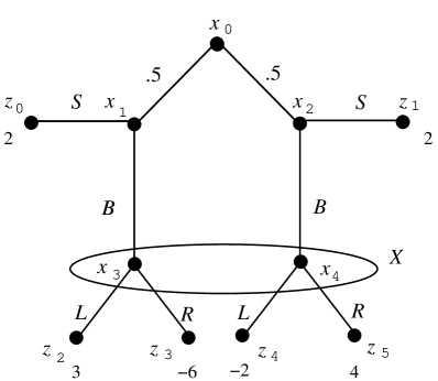
Figure 1: A game of imperfect recall.

It is not hard to show that the strategy that maximizes expected utility chooses action $S$ at node $x_{1}$, action $B$ at node $x_{2}$, and action $R$ at the information set $X$ consisting of $x_{3}$ and $x_{4}$. Call this strategy $f$. Suppose that the agent uses strategy $f$. If the agent knows his strategy (the typical assumption in game theory), then the agent knows, when he is at the information set $X$, then he must be at $x_{4}$. So in what sense are $x_{3}$ and $x_{4}$ in the same information set?

Halpern [?] already observes that, in order to analyze games of imperfect recall, we must make explicit what an agent knows (including things like whether he knows his strategy, and whether he recalls that he has switched strategies). These issues are made explicit when we consider TMs, and take an agent’s information set to be determined by the state of his TM—the state explicitly determines what the agent knows (and remembers). Furthemore, although the information sets are determined by the TM chosen by the agent, we can force the agent into a situation of imperfect recall by “charging” a lot for memory. Thus, our computational model generalizes standard models of imperfect recall (and also perfect recall) while providing an, in our eyes, more natural and explicit formalization of the game.

Games like that in Figure 1 are just an example of the subtleties that must be dealt with when defining sequential equilibrium in We give a definition of sequential equilibrium in a companion paper [Halpern and Pass 2011b] for standard games of imperfect recall that we extend here to take computation into account. We show that, in general, sequential equilibrium does not exist, but give simple conditions that guarantee that it exists, as long as a NE (Nash equilibrium) exists. (As is shown by a simple example in [Halpern and Pass 2011a], reviewed below, NE is not guaranteed to exist in machine games, although sufficient conditions are given to guarantee existence.)

The definition of sequential equilibrium in [Halpern and Pass 2011b] views sequential equilibrium as an ex ante notion. The idea is that a player chooses his strategy before the game starts and is committed to it, but he chooses it in such a way that it remains optimal even off the equilibrium path. This, unfortunately, does not correspond to the more standard intuitions behind sequential equilibrium, where players are reconsidering at each information set whether they are doing the “right” thing, and if not, can change their strategies. This interim notion of sequential rationality agrees with the ex ante notion in games of perfect recall, but the two notions differ in games of imperfect recall. We argue in [Halpern and Pass 2011b] there are some deep conceptual problems with the interim notion in standard games of imperfect recall. We consider both an ex ante and interim notion of sequential equilibrium here. We show that the conceptual problems when the game tree is given (as it is in standard games) largely disappear when the game tree (and, in particular, the information sets) are determined by the TM chosen, as is the case in machine games. Moreover, we show that, under natural assumptions regarding the complexity function, the two notions coincide.

The rest of this paper is organized as follows. In Section 2, we review the relevant definitions of Bayesian machine game from [Halpern and Pass 2011a]. In Section 3 we show how we can view these Bayesian machine games as extensive-form games, where the players moves involve computation. In Sections 4 we define beliefs in Bayesian machine games; using this definition, we define interim and ex ante sequential equilibrium in Section 5, and provide a natural condition under which they are equivalent. In Section 6, we relate Nash equilibrium and sequential equilibrium. Not surprisingly, every sequential equilibrium in a Nash equilibrium; we provide a natural condition under which a Nash equilibrium is an ex ante sequential equilibrium. In Section 7, we consider when sequential equilibrium exists. Since, as shown in [Halpern and Pass 2011a], even Nash equilibrium may not exist in Bayesian machine games, we clearly cannot expect a sequential equilibrium to exist in general. We show that if the set of TMs that the agents can choose from is finite, then an ex ante sequential equilibrium exists whenever a Nash equilibrium does; we also provide a natural sufficient condition for an ex ante sequential equilibrium to exist even if the set of TMs the agents can choose from is infinite. Up to this point in the paper, we have considered only extensive-form games determined by Bayesian machine games, where players make only one move in the underlying Bayesian game, and the remaining moves correspond to computation steps. In Section 8, we extend our definitions to cases where the underlying game is an extensive-form game. We conclude in Section 9 with some discussion.

2 Computational games: a review

This review is largely taken from [Halpern and Pass 2011a]. We model costly computation using Bayesian machine games. Formally, a Bayesian machine game is given by a tuple $([m],{\cal M},T,\Pr,$ $\mathscr{C}_{1},\ldots,\mathscr{C}_{m},u_{1},\ldots,u_{m})$, where

• $[m]=\{1,\ldots,m\}$ is the set of players;

• ${\cal M}$ is a set of TMs;

• ${T}\subseteq(\{0,1\}^{*})^{m}$ is the set of type profiles ($m$-tuples consisting of one type for each of the $m$ players);

• $\Pr$ is a distribution on ${T}$;

• $\mathscr{C}_{i}$ is a complexity function (see below);

• $u_{i}:{T}\times(\{0,1\}^{*})^{m}\times\mbox{$I\!\!N$}^{m}\rightarrow\mbox{$I\!\!R$}$ is player $i$’s utility function. Intuitively, $u_{i}(\vec{t},\vec{a},\vec{c})$ is the utility of player $i$ if $\vec{t}$ is the type profile, $\vec{a}$ is the action profile (where we identify $i$’s action with $M_{i}$’s output), and $\vec{c}$ is the profile of machine complexities.

If we ignore the complexity function and drop the requirement that an agent’s type is in $\{0,1\}^{*}$, then we have the standard definition of a Bayesian game. We assume that TMs take as input strings of 0s and 1s and output strings of 0s and 1s. Thus, we assume that both types and actions can be represented as elements of $\{0,1\}^{*}$. We allow machines to randomize, so given a type as input, we actually get a distribution over strings. To capture this, we take the input to a TM to be not only a type, but also a string chosen with uniform probability from $\{0,1\}^{\infty}$ (which we view as the outcome of an infinite sequence of coin tosses). The TM’s output is then a deterministic function of its type and the infinite random string. We use the convention that the output of a machine that does not terminate is a fixed special symbol $\omega$. We define a view to be a pair $(t,r)$ of two bitstrings; we think of $t$ as that part of the type that is read, and of $r$ as the string of random bits used. A complexity function $\mathscr{C}:{\bf M}\times\{0,1\}^{*};(\{0,1\}^{*}\cup\{0,1\}^{\infty})\rightarrow\mbox{$I\!\!N$}$, where ${\bf M}$ denotes the set of Turing machines, gives the complexity of a (TM,view) pair.

We can now define player $i$’s expected utility $U_{i}(\vec{M})$ if a profile $\vec{M}$ of TMs is played; we omit the standard details here. We then define a (computational) NE of a machine game in the usual way:

Definition 2.1

Given a Bayesian machine game $G=([m],{\cal M},T,\Pr,\vec{\mathscr{C}},\vec{u})$, a machine profile $\vec{M}\in{\cal M}^{m}$ is a (computational) Nash equilibrium if, for all players $i$, $U_{i}(\vec{M})\geq U_{i}(M_{i}^{\prime},\vec{M}_{-i})$ for all TMs $M_{i}^{\prime}\in{\cal M}$.

Although a NE always exists in standard games, a computational NE may not exist in machine games, as shown by the following example, taken from [Halpern and Pass 2011a].

Example 2.2

Consider rock-paper-scissors. As usual, rock beats scissors, scissors beats paper, and paper beats rock. A player gets a payoff of 1 if he wins, $-1$ if he loses, and 0 if it is a draw. But now there is a twist: since randomizing is cognitively difficult, we charge players $\epsilon>0$ for using a randomized strategy (but do not charge for using a deterministic strategy). Thus, a player’s payoff is $1-\epsilon$ if he beats the other player but uses a randomized strategy. It is easy to see that every strategy has a deterministic best response (namely, playing a best response to whatever move of the other player has the highest probability); this is a strict best response, since we now charge for randomizing. It follows that, in any equilibrium, both players must play deterministic strategies (otherwise they would have a profitable deviation). But there is clearly no equilibrium where players use deterministic strategies.  

Interestingly, it can also be shown that, in a precise sense, if there is no cost for randomization, then a computational NE is guaranteed to exist in a computable Bayesian machine game (i.e., one where all the relevant probabilities are computable); see [Halpern and Pass 2011a] for details.

3 Computation as an extensive-form game

Recall that a deterministic TM $M=(\tau,{Q},q_{0},{\cal H})$ consists of a read-only input tape, a write-only output tape, a read-write work tape, 3 machine heads (one reading each tape), a set ${Q}$ of machine states, a transition function $\tau:{Q}\times\{0,1,b\}^{2}\rightarrow{Q}\times\{0,1,b\}^{2}\times\{L,R,S\}^{3}$, an initial state $q_{0}\in{Q}$, and a set ${\cal H}\subseteq{Q}$ of “halt” states. We assume that all the tapes are infinite, and that only 0s, 1s and blanks (denoted $b$) are written on the tapes. We think of the input to a TM as a string in $\{0,1\}^{*}$ followed by blanks. Intuitively, the transition function says what the TM will do if it is in a state $s$ and reads $i$ on the input tape and $j$ on the work tape. Specifically, $\tau$ describes what the new state is, what symbol is written on the work tape and the output tape, and which way each of the heads moves ($L$ for one step left, $R$ for one step right, or $S$ for staying in the same place). The TM starts in state $q_{0}$, with the input written on the input tape, the other tapes blank, the input head at the beginning of the input, and the other heads at some canonical position on the tapes. The TM then continues computing according to $\tau$. The computation ends if and when the machine reaches a halt state $q\in{\cal H}$. To simplify the presentation of our results, we restrict attention to TMs that include only states $q\in{Q}$ that can be reached from $q_{0}$ on some input. We also consider randomized TMs, which are identical to deterministic TMs except that the transition function $\tau$ now maps ${Q}\times\{0,1,b\}^{2}$ to a probability distribution over ${Q}\times\{0,1,b\}^{2}\times\{L,R,S\}^{3}$. As is standard in the computer science literature, we restrict attention to probability distributions that can be generated by tossing a fair coin; that is, the probability of all outcomes has the form $c/2^{k}$ for $c,k\in\mbox{$I\!\!N$}$.

In a standard extensive-form game, a strategy is a function from information sets to actions. Intuitively, in a state $s$ in an information set $I$ for player $i$, the states in $I$ are the ones that $i$ considers possible, given his information at $s$; moreover, at all the states in $I$, $i$ has the same information. In the “runs-and-systems” framework of Fagin et al. [?], each agent is in some local state at each point in time. A protocol for agent $i$ is a function from $i$’s local states to actions. We can associate with a local state $\ell$ for agent $i$ all the histories of computation that end in that local state; this can be thought of as the information set associated with $\ell$. With this identification, a protocol can also be viewed as a function from information sets to actions, just like a strategy.

In our setting, the closest analogue to a local state in the runs-and-systems framework is the state of the TM. Intuitively, the TM’s state describes what the TM knows. The transition function $\tau$ of the TM determines a protocol, that is, a function from the TM’s state to a “generalized action”, consisting of reading the symbols on its read and work tapes, then moving to a new state and writing some symbols on the write and work tapes (perhaps depending on what was read). We can associate with a state $q$ of player $i$’s TM the information set $I_{q}$ consisting of all histories $h$ where player $i$’s is in state $q$ at the end of the history. (Here, a history is just a sequence of extended state profiles, consisting of one extended state for each player, and an extended state for player $i$ consists of the TM that $i$ is using, the TM’s state, and the content and head position of each of $i$’s tapes.) Thus, player $i$ implicitly chooses his information sets (by choosing the TM), rather than the information set being given exogenously.

The extensive-form game defined by computation in a Bayesian machine game is really just a collection of $m$ single-agent decision problems. Of course, sequential equilibrium becomes even more interesting if we consider computational extensive-form games, where there is computation going on during the game, and we allow for interaction between the agents. It turns out that many of the issues of interest already arise in our setting.

4 Beliefs

Using the view of machine games as extensive-form games, we can define sequential equilibrium. The first step to doing so involves defining a player’s beliefs at an information set. But now we have to take into account that the information set is determined by the TM chosen. In the spirit of Kreps and Wilson [?], define a belief system $\mu$ for a game $G$ to be a function that associates with each player $i$, TM $M_{i}$ for player $i$, and a state $q$ for $M_{i}$ a probability on the histories in the information set $I_{q}$. Following [Halpern and Pass 2011b], we interpret $\mu_{q,M_{i}}(x)$ as the probability of going through history $x$ conditional on reaching the local state $q$.

We do not expect $\sum_{x\in I_{q}}\mu_{q,M_{i}}(x)$ to be $1$; in general, it is greater than 1. This point is perhaps best explained in the context of games of imperfect recall. Let the upper frontier of an information set $X$ in a game of imperfect recall, denoted $\hat{X}$, consist of all those histories $h\in X$ such that there is no history $h^{\prime}\in X$ that is a prefix of $h$. In [Halpern and Pass 2011b], we consider belief systems that associate with each information set $X$ a probability $\mu_{X}$ on the histories in $X$. Again, we do not require $\sum_{h\in X}\mu_{X}(h)=1$. For example, if all the histories in $X$ are prefixes of same complete history $h^{*}$, then we might have $\mu_{X}(h)=1$ for all histories $h\in X$. However, we do require that $\Sigma_{h\in\hat{X}}\mu_{X}(h)=1$. We make the analogous requirement here. Let $\hat{I}_{q}$ denote the upper frontier of $I_{q}$. The following lemma, essentially already proved in [Halpern and Pass 2011b], justifies the requirement.

Lemma 4.1

If $q$ is a local state for player $i$ that is reached by $\vec{M}$ with positive probability, and $\mu_{q}^{\prime}(h)$ is the probability of going through history $h$ when running $\vec{M}$ conditional on reaching $q$, then $\sum_{h\in\hat{I}_{q}}\mu_{q}^{\prime}(h)=1$.

Given a belief system $\mu$ and a machine profile $\vec{M}$, define a probability distribution $\mu^{\vec{M}}_{q}$ over terminal histories in the obvious way: for each terminal history $z$, let $h_{z}$ be the history in $\hat{I}_{q}$ generated by $\vec{M}$ that is a prefix of $z$ if there is one (there is clearly at most one), and define $\mu^{\vec{M}}_{q}(z)$ as the product of $\mu_{q,M_{i}}(h_{z})$ and the probability that $\vec{M}$ leads to the terminal history $z$ when started in $h_{z}$; if there is no prefix of $z$ in $I_{q}$, then $\mu^{\vec{M}}_{q}(z)=0$. Following Kreps and Wilson [?], let $U_{i}(\vec{M}\mid q,\mu)$ denote the expected utility for player $i$, where the expectation is taken with respect to $\mu^{\vec{M}}_{q}$. Note that utility is well-defined, since a terminal history determines both the input and the random-coin flips of each player’s TM, and thus determines both its output and complexity.

5 Defining sequential equilibrium

If $q$ is a state of TM $M_{i}$, we want to capture the intuition that a TM $M_{i}$ for player $i$ is a best response to a machine profile $\vec{M}_{-i}$ for the remaining players at $q$ (given beliefs $\mu$). Roughly speaking, we capture this by requiring that the expected utility of using another TM $M^{\prime}_{i}$ starting at a node where the TM’s state is $q$ to be no greater than that of using $M_{i}$. “Using a TM $M^{\prime}_{i}$ starting from $q$” means using the TM $(M_{i},q,M_{i}^{\prime})$, which, roughly speaking, is the TM that runs like $M_{i}$ up to $q$, and then runs like $M^{\prime}_{i}$.

In the standard setting, all the subtleties in the definition of sequential equilibrium involve dealing with what happens at information sets that are reached with probability 0. When we consider machine games, as we shall see, under some reasonable assumptions, all states are reached with positive probability in equilibrium, so dealing with probability 0 is not a major concern (and, in any case, the same techniques that are used in the standard setting can be applied). But there are several new issues that must be addressed in making precise what it means to “switch” from $M_{i}$ to $M_{i}^{\prime}$ at $q$.

Given a TM $M_{i}=(\tau,{Q},q_{0},{\cal H})$ and $q\in{Q}$, let ${Q}_{q,M_{i}}$ consist of all states $q^{\prime}\in{Q}$ such that, for all views $v$, if the computation of $M_{i}$ given view $v$ reaches $q^{\prime}$, then it also reaches $q$. We can think of ${Q}_{q,M_{i}}$ as consisting of the states $q^{\prime}$ that are “necessarily” below $q$, given that $M_{i}$ is used. Note that $q\in{Q}_{q,{M_{i}}}$. Say that $M_{i}^{\prime}=(\tau^{\prime},{Q}^{\prime},q^{\prime},{\cal H}^{\prime})$ is compatible with $M_{i}$ given $q$ if $q^{\prime}=q$ (so that $q$ is the start state of $M_{i}^{\prime}$) and $\tau$ and $\tau^{\prime}$ agree on all states in ${Q}-{Q}_{q,M_{i}}$. If $M_{i}^{\prime}$ is not compatible with $M_{i}$ given $q$, then $(M_{i},q,M_{i}^{\prime})$ is not well defined. If $M_{i}^{\prime}$ is compatible with $M_{i}$ given $q$, then $(M_{i},q,M_{i}^{\prime})$ is the TM $({Q}^{\prime\prime},[\tau,q,\tau^{\prime}],q_{0},{\cal H}^{\prime\prime})$, where ${Q}^{\prime\prime}=({Q}-{Q}_{q,M_{i}})\cup{Q}^{\prime}$; $[\tau,q,\tau^{\prime}]$ is the transition function that agrees with $\tau$ on states in ${Q}-{Q}_{q,M_{i}}$, and agrees with $\tau^{\prime}$ on the remaining states; and ${\cal H}^{\prime\prime}=({\cal H}\cap({Q}-{Q}_{q,M_{i}}))\cup{\cal H}^{\prime}$.

Since $(M_{i},q,M_{i}^{\prime})$ is a TM, its complexity given a view is well defined. In general, the complexity of $(M_{i},q,M_{i}^{\prime})$ may be different from that of $M_{i}$ even on histories that do not go through $q$. For example, consider a one-person decision problem where the agent has an input (i.e., type) of either 0 or 1. Consider four TMs: $M$, $M_{0}$, $M_{1},$ and $M^{*}$. Suppose that $M$ embodies a simple heuristic that works well on both inputs, $M_{0}$ and $M_{1}$ give better results than $M$ if the inputs are 0 and 1, respectively, and $M^{*}$ acts like $M_{0}$ if the input is 0 and like $M_{1}$ if the input is 1. Clearly, if we do not take computational costs into account, $M^{*}$ is a better choice than $M$; however, suppose that with computational costs considered, $M$ is better than $M_{0}$, $M_{1}$, and $M^{*}$. Specifically, suppose that $M_{0}$, $M_{1}$, and $M^{*}$ all use more states than $M$, and the complexity function charges for the number of states used. Now suppose that the agent moves to state $q$ if he gets an input of 0. In state $q$, using $M_{0}$ is better than continuing with $M$: the extra charge for complexity is outweighed by the improvement in performance. Should we say that using $M$ is then not a sequential equilibrium? The TM $(M,\{q\},M_{0})$ acts just like $M_{0}$ if the input is 0. From the ex ante point of view, $M$ is a better choice than $M_{0}$. However, having reached $q$, the agent arguably does not care about the complexity of $M_{0}$ on input 1. Our definition of ex ante sequential equilibrium restricts the agent to making changes that leave unchanged the complexity of paths that do not go through $q$ (and thus would not allow a change to $M_{0}$ at $q$). Our definition of interim sequential equilibrium does not make this restriction; this is the only way that the two definitions differ.Note that this makes it easier for a strategy to be an ex ante sequential equilibrium (since fewer deviations are considered).

$(M_{i},q,M_{i}^{\prime})$ is a local variant of $M_{i}$ if the complexity of $(M_{i},q,M_{i}^{\prime})$ is the same as that of $M_{i}$ on views that do not go through $q$; that is, if for every view $v$ such that the computation of $M_{i}(v)$ does not reach $q$, $\mathscr{C}(M_{i},v)=\mathscr{C}((M_{i},q,M_{i}^{\prime}),v)$. A complexity function $\mathscr{C}$ is local if $\mathscr{C}(M_{i},v)=\mathscr{C}((M_{i},q,M_{i}^{\prime}),v)$ for all TMs $M_{i}$ and $M_{i}^{\prime}$, states $q$, and views $v$ that do not reach $q$. Clearly a complexity function that considers only running time, space used, and the transitions undertaken on a path is local. If $\mathscr{C}$ also takes the number of states into account, then it is local as long as $M_{i}$ and $(M_{i},q,M_{i}^{\prime})$ have the same number of states. Indeed, if we think of the state space as “hardware” and the transition function as the “software” of a TM, then restricting to changes $M_{i}^{\prime}$ that have the same state space as $M_{i}$ seems reasonable: when the agent contemplates making a change at a non-initial state, he cannot acquire new hardware, so he must work with his current hardware.

A TM $M_{i}=(\tau,{Q},q_{0},{\cal H})$ for player $i$ is completely mixed if, for all states $q\in{Q}-{\cal H}$, $q^{\prime}\in{Q}$, and bits $k,k^{\prime}\in\{0,1\}$, $\tau(q,k,k^{\prime})$ assigns positive probability to making a transition to $q^{\prime}$. A machine profile $\vec{M}$ is completely mixed if for each player $i$, $M_{i}$ is completely mixed. Following Kreps and Wilson [?], we would like to say that a belief system $\mu$ is compatible with a machine profile $\vec{M}$ if there exists a sequence of completely-mixed machine profiles $\vec{M^{1}},\vec{M^{2}},\ldots$ converging to $\vec{M}$ such that if $q$ is a local state for player $i$ that is reached with positive probability by $\vec{M}$ (that is, there is a type profile $\vec{t}$ that has positive probability according to the type distribution in $G$ and a profile $\vec{r}$ of random strings such that $\vec{M}(\vec{t},\vec{r})$ reaches $q$), then $\mu_{q,M_{i}}(h)$ is just the probability of $\vec{M}$ going through $h$ conditional on $\vec{M}$ reaching $q$ (denoted $\pi_{\vec{M}}(h\mid q)$); and if $q$ is a local state that is reached with probability 0 by $\vec{M}$, then $\mu_{q,M_{i}}(h)$ is $\lim_{n\rightarrow\infty}\pi_{\vec{M}^{n}}(h\mid q)$. To make this precise, we have to define convergence. We say that $\vec{M^{1}},\vec{M^{2}},\ldots$ converges to $\vec{M}$ if, for each player $i$, all the TMs $M^{1}_{i},{M^{2}_{i}},\ldots,{M_{i}}$ have the same state space, and the transition function of each TM in the sequence to converge to that of $M_{i}$. Note that we place no requirement on the complexity functions. We could require the complexity function of $M_{i}^{k}$ to converge to that of $M_{i}$ in some reasonable sense. However, this seems to us unreasonable. If we assume that randomization is free (in the sense hinted at after Example 2.2), then the convergence of the complexity functions follows from the convergence of the transition functions. On the other hand, if we have a complexity function that charges for randomization, as in Example 2.2, then the complexity functions of $M_{i}^{n}$ may not converge to the complexity function of $M_{i}$. Thus, if we require the complexity functions to converge, there will not be a sequence of completely mixed strategy profiles converging to a deterministic strategy profile $\vec{M}$. If we think of the sequence of TMs as arising from “trembles” in the operation of some fixed TM (e.g., due to machine failure), then requiring that the complexity functions converge seems unreasonable.

Definition 5.1

A pair $(\vec{M},\mu)$ consisting of a machine profile $\vec{M}$ and a belief system $\mu$ is called a belief assessment. A belief assessment $(\vec{M},\mu)$ is an interim sequential equilibrium (resp., ex ante sequential equilibrium) in a machine game $G=([m],{\cal M},\ldots)$ if $\mu$ is compatible with $\vec{M}$ and for all players $i$, states $q$ of $M_{i}$, and TMs $M^{\prime}_{i}$ compatible with $M_{i}$ and $q$ such that $(M_{i},q,M^{\prime}_{i})\in{\cal M}$ (resp., and $(M_{i},q,M^{\prime}_{i})$ is a local variant of $M_{i}$), we have

$$U_{i}(\vec{M}\mid q,\mu)\geq U_{i}(((M_{i},q,M^{\prime}_{i}),\vec{M}_{-i})\mid q,\mu)).$$

Note that in Definition 5.1 we consider only switches $(M_{i},q,M^{\prime}_{i})$ that result in a TM that is in the set ${\cal M}$ of possible TMs in the game. That is, we require that the TM we switch to is “legal”, and has a well-defined complexity.

As we said, upon reaching a state $q$, an agent may well want to switch to a TM $(M_{i},q,M^{\prime}_{i})$ that is not a local variant of $M_{i}$. This is why we drop this requirement in the definition of interim sequential equilibrium. But it is a reasonable requirement ex ante. It means that, at the planning stage of the game, there is no TM $M_{i}^{\prime}$ and state $q$ such that agent $i$ prefers to use $M^{\prime}_{i}$ in the event that $q$ is reached. That is, $M_{i}$ is “optimal” at the planning stage, even if the agent considers the possibility of reaching states that are off the equilibrium path.

The following result is immediate from the definitions, and shows that, in many cases of interest, the two notions of sequential equilibrium coincide.

Proposition 5.2

Every interim sequential equilibrium is an ex ante sequential equilibrium. In a machine game with a local complexity function, the interim and ex ante sequential equilibria coincide.

As the discussion above emphasizes, a host of new issues arise when defining sequential equilibrium in the context of machine games. While we believe we have made reasonable choices, variants of our definitions are also worth considering. For instance, our way of defining beliefs in the definition of interim sequential equilibrium arguably still has an ex ante flavor (recall that the probability assigned to a node in an information set is the probability of reaching the node conditioned on reaching the information set). If we want these beliefs to instead correspond to the probabilities the agent assigns to being at the node, conditioned on being at the information set, we need to consider more carefully when the agent reconsiders his strategy. If the decision to reconsider depends only on the information set, then the change in strategy must happen at the upper frontier of the information set, that is, when the information set is first reached, and our current analysis of interim sequential seems reasonable. If the change does not necessarily happen at the upper frontier, then we need to model under what circumstances reconsideration occurs. (This point is also made in [GroveHalpern95, Halpern 1997].) For concreteness, in our context, assume that at each step of the computation, with some small probability $\epsilon$, a human (the agent) comes in, observes the state of the TM, and decides whether it wishes to switch machines

Such a model would result in a different way of ascribing beliefs. Our results no longer apply if we use this alternative way of ascribing beliefs: it is not hard to come up with a machine game that corresponds to the “absentminded-driver” game of [Piccione and Rubinstein 1997] where a Nash equilibrium exists, the complexity function is local, but no interim sequential equilibrium exists using this method to ascribe beliefs.

6 Relating Nash equilibrium and sequential equilibrium

In this section, we relate NE and sequential equilibrium.

First note that is easy to see that every (computational) sequential equilibrium is a NE, since if $q=q_{0}$, the start state, $(M_{i},q_{0},M_{i}^{\prime})=M_{i}^{\prime}$. That is, by taking $q=q_{0}$, we can consider arbitrary modifications of the TM $M_{i}$.

Proposition 6.1

Every ex ante sequential equilibrium is a NE.

Of course, since every interim sequential equilibrium is an ex ante sequential equilibrium, it follows that every interim sequential equilibrium is a NE as well.

In general, not every NE is a sequential equilibrium. However, under some natural assumptions on the complexity function, the statement holds. A strategy profile $\vec{M}$ in a machine game $G$ is lean if, for all players $i$ and local states $q$ of $M_{i}$, $q$ is reached with positive probability when playing $\vec{M}$. The following proposition is the analogue of the well-known result that, with the traditional definition of sequential equilibrium, every completely mixed NE is also a sequential equilibrium.

Proposition 6.2

If $\vec{M}$ is a lean NE for machine game $G$ and $\mu$ is a belief system compatible with $\vec{M}$, then $(\vec{M},\mu)$ is an ex ante sequential equilibrium.

Proof:  We need to show only that for each player $i$ and local state $q$ of $M_{i}$, there does not exist a TM $M^{\prime}_{i}$ compatible with $(M_{i},q)$ such that $U_{i}(\vec{M}\mid q,\mu)<U_{i}(((M_{i},q,M^{\prime}_{i}),\vec{M}_{-i})\mid q,\mu).$ Suppose by way of contradiction that there exist such a TM $M^{\prime}_{i}$ and local state $q$. Since $\mu$ is compatible with $\vec{M}$, it follows that $U_{i}(\vec{M}\mid q)<U_{i}(((M_{i},q,M^{\prime}_{i}),\vec{M}_{-i})\mid q).$ Since $(M_{i},q,M_{i}^{\prime})$ is local variant of $M_{i}$, $U_{i}(\vec{M}\mid\text{not reaching }q)=U_{i}(((M_{i},q,M^{\prime}_{i}),\vec{M}_{-i})\mid\text{not reaching }q)).$ By the definition of $(M_{i},q,M^{\prime}_{i})$, the probability that $M_{i}$ and $(M_{i},q,M^{\prime}_{i})$ reach $q$ is identical; it follows that $U_{i}(\vec{M})<U_{i}((M_{i},q,M^{\prime}_{i}),\vec{M}_{-i})$, which contradicts the assumption that $\vec{M}$ is a NE.  

The restriction to local variants $(M_{i},q,M_{i}^{\prime})$ of $M_{i}$ in the definition of ex ante sequential equilibrium is critical here. Proposition 6.2 does not hold for interim sequential equilibrium. Suppose, for example, that if $i$ is willing to put in more computation at $q$, then he gets a better result. Looked at from the beginning of the game, it is not worth putting in the extra computation, since it involves using extra states, and this charge is global (that is, it affects the complexity of histories that do not reach $q$). But once $q$ is reached, it is certainly worth putting in the extra computation. If we assume locality, then the extra computational effort at $q$ does not affect the costs for histories that do not go through $q$. Thus, if it is worth putting in the effort, it will be judged worthwhile ex ante. The following two examples illustrate the role of locality.

Example 6.3

Let $x$ be an $n$-bit string whose Kolmogorov complexity is $n$ (i.e., $x$ is incompressible—there is no shorter description of $x$). Consider a single-agent game $G_{x}$ (so the $x$ is built into the game; it is not part of the input) where the agent’s type is a string of length $\log n$, chosen uniformly at random, and the utility function is defined as follows, for an agent with type $t$:

• The agent “wins” if it outputs $(1,y)$, where $y=x_{t}$ (i.e., it manages to guess the $t$th bit of $x$, where $t$ is its type). In this case, it receives a utility of $10$, as long as its complexity is at most 2.

• The agent can also “give up”: if it outputs $t_{0}$ (i.e., the first bit of its type) and its complexity is 1, then it receives a utility of 0.

• Otherwise, its utility is $-\infty$.

Consider the 4-state TM $M$ that just “gives up”. Formally, $M=(\tau,\{q_{0},b_{0},b_{1},H\},q_{0},\{H\})$, where $\tau$ is such that, in $q_{0}$, $M$ reads the first bit $t_{0}$ of the type, and transitions to $b_{i}$ if it is $i$; and in state $b_{i}$, it outputs $i$ and transitions to $H$, the halt state. Now define the complexity function as follows:

• the complexity of $M$ is $1$ (on all inputs);

• the complexity of any TM $M^{\prime}\neq M$ that has at most $0.9n$ states is $2$;

• all other TMs have complexity 3.

Note that $M$ is the unique NE in $G_{x}$. Since $x$ is incompressible, no TM $M^{*}$ with fewer than $0.9n$ states can correctly guess $x_{t}$ for all $t$ (for otherwise $M^{*}$ would provide a description of $x$ shorter than $|x|$). It follows that no TM with complexity greater than 1 does better than $M$. Thus, $M$ is the unique NE. It is also a lean NE, and thus, by Proposition 6.2, an ex ante sequential equilibrium. However, there exists a non-local variant of $M$ at $b_{0}$ that gives higher utility than $M$. Notice that if the first bit is 0 (i.e., if the TM is in state $b_{0}$), then $x_{t}$ is one of the first $n/2$ bits of $x$. Thus, at $b_{0}$, we can switch to the TM $M^{\prime}$ that reads the whole type $t$ and the first $n/2$ bits of $x$, outputs $(1,x_{t})$. It is easy to see that $M^{\prime}$ can be constructed using $0.5n+O(1)$ states. Thus, $M$ is not an interim sequential equilibrium (in fact, none exists in $G_{x}$). $(M,b_{0},M^{\prime})$ is not a local variant of $M$, since $M^{\prime}$ has higher complexity than $M$ at $q_{0}$.  

Example 6.4

Consider the game in Figure 1 again. Recall that the strategy that maximizes expected utility is the strategy $f$ that chooses action $S$ at node $x_{1}$, action $B$ at node $x_{2}$, and action $R$ at the information set $X$ consisting of $x_{3}$ and $x_{4}$. Let $f^{\prime}$ be the strategy of choosing action $B$ at $x_{1}$, action $S$ at $x_{2}$, and $L$ at $X$. As Piccione and Rubinstein point out, if node $x_{1}$ is reached and the agent is using $f$, then he will not want to continue using $f$; he would prefer to switch to $f^{\prime}$ instead. In the language of this paper, $f$ is not an interim sequential equilibrium, although it is a NE of the one-player game. Note that $f^{\prime}$ is neither a NE nor an interim sequential equilibrium (since if the player is using $f^{\prime}$ at $x_{2}$, he will want to switch to $f$). According to the definition in [Halpern and Pass 2011b], $f$ is an ex ante sequential equilibrium. The reason is that switching from $f$ to $f^{\prime}$ is not allowed at $x_{1}$, because $f^{\prime}$ does something different from $f$ at a node that is not below $x_{1}$, namely $x_{4}$. As a consequence, $(f,x,f^{\prime})$ is not a strategy in the game, since it does different things at $x_{3}$ and $x_{4}$, although they are in the same information set. The requirement made in [Halpern and Pass 2011b] that, when considering switching from a strategy $f$ to $f^{\prime}$ at an information set $X^{*}$, $f^{\prime}$ has to agree with $f$ at all nodes not below $X^{*}$ is somewhat analogous to the local-variant requirement that we make here in the definition of ex ante sequential equilibrium.

We now consider a machine game that captures some of the essential features of the game in Figure 1. Suppose that there are two types, 0 and 1, which each occurs with probability $1/2$. The agent must choose between two TMs, $M_{0}$ and $M_{1}$, which can be viewed as corresponding to $f$ and $(f,x,f^{\prime})$. $M_{0}$ reads the input in state $q_{0}$, and moves to either state $q_{1}$ or $q_{2}$, depending on whether it reads 0 or 1. In $q_{1}$, $M_{0}$ moves to state $H$, the halt state, outputting nothing (i.e., the output is $b$, the blank symbol). In state $q_{2}$, $M_{0}$ writes 1 on its output tape and moves to $q_{4}$; in $q_{4}$, it writes 1 again, and moves to $H$. $M_{1}$ again moves to $q_{1}$ or $q_{2}$ depending on its input, and from $q_{2}$ moves to $q_{4}$ and $H$, writing $11$, just like $M_{0}$. But from $q_{2}$, it moves to $q_{3}$ and $H$, writing $00$.

The payoffs are as follows: if the output is $b$, the payoff is $2-c$ for both inputs, where $c$ is the complexity of the machine chosen. If the output is $00$ and the input is $0$, the payoff is $3-c$; if the output is $11$ and the input is $1$, the payoff is $4-c$. If the output is something other than $b$ or $00$ and the input is 0, then the payoff is $-6$; if the output is something other than $b$ or $11$ and the input is 1, then the payoff of $-2$. Finally, $c=0$ if $M_{0}$ is chosen, and $c=.75$ if $M_{1}$ is chosen.

It is easy to see that $M_{0}$ is a NE; its expected payoff is 3, while that of $M_{1}$ is $2.75$. However, $M_{0}$ is not an interim sequential equilibrium, because at $q_{1}$, the agent prefers switching to $(M_{0},q_{1},M_{1})$, which is equivalent to $M_{1}$, since, conditional on reaching $q_{1}$, the expected payoff of $M_{0}$ is $2$, while that of $M_{1}$ is $2.25$. Note that although $(f,x_{1},f^{\prime})$ is not a strategy, $(M_{0},q_{1},M_{1})$ is a TM (and is equivalent to $M_{1}$). Switching from $M_{0}$ to $(M_{0},q_{1},M_{1})$ results in changing the information strucure. Such a change is not possible in standard games of imperfect recall. Finally, note that $M_{0}$ is an ex ante sequential equilibrium; the switch from $M_{0}$ to $(M_{0},q_{1},M_{1})$ is disallowed at $q_{1}$ because $(M_{0},q_{1},M_{1})$ is not a local variant of $M_{0}$.  

We now show that for a natural class of games, every NE is lean, and thus also an ex ante sequential equilibrium. Intuitively, we consider games where there is a strictly positive cost for having more states. Our argument is similar in spirit to that of Rubinstein [?], who showed that in his games with automata, there is always a NE with no “wasted” states; all states are reached in equilibrium. Roughly speaking, a machine game $G$ has positive state cost if (a) a state $q$ is not reached in TM $M$, and $M^{-q}$ is the TM that results from removing $q$ from $M$, then $\mathscr{C}_{i}(M^{-q},v)<\mathscr{C}_{i}(M,v)$; and (b) utilities are monotone decreasing in complexity; that is, $u_{i}(\vec{t},\vec{a},(c^{\prime}_{i},\vec{c}_{-i}))<u_{i}(\vec{t},\vec{a},(c_{i},\vec{c}_{i}))$ if $c^{\prime}_{i}>c_{i}$. More precisely, we have the following definition.

Definition 6.5

A machine game $G=([m],{\cal M},\Pr,\vec{\mathscr{C}},\vec{u})$ has positive state cost if the following two conditions hold:

• For all players $i$, TMs $M_{i}=(\tau,{Q},q_{0},{\cal H})$, views $v$ for player $i$, and local states $q\neq q_{0}$ in ${Q}$ such that $q$ is not reached in view $v$ when running $M_{i}$ (note that because the view gives the complete history of messages received and read, we can compute the sequence of states that player $i$ goes through when using $M_{i}$ if his view is $v$), $\mathscr{C}_{i}(M^{-q},v)<\mathscr{C}_{i}(M,v)$, where $M^{-q}=({Q}-\{q\},\tau^{q},q_{0})$, and $\tau^{q}$ is identical to $\tau$ except that all transition to $q$ are replaced by transitions to $q_{0}$.

• Utilities are monotone decreasing in complexity; that is, for all players $i$, type profiles $\vec{t}$, action profiles $\vec{a}$, and complexity profiles $(c_{i},\vec{c}_{-i})$, views $v$, $(c^{\prime}_{i},\vec{c}_{-i})$, if $c^{\prime}_{i}>c_{i}$, then $\mathscr{C}_{i}(M^{-q},v)<\mathscr{C}_{i}(M,v)$.

Lemma 6.6

Every NE $\vec{M}$ for machine game $G$ with positive state cost is lean.

Proof:  Suppose, by way of contradiction, that there exists a NE $\vec{M}$ for a game $G$ with positive state cost, a player $i$, and a local state $q$ of $M_{i}$ that is reached with probability $0$. First, note that $q$ cannot be the initial state of $M_{i}$, since, by definition, the initial state of every TM is reached with probability 1. Since $g$ has positive state cost, for every view $v$ that is assigned positive probability (according to the type distribution of $G$), $M_{i}^{-q}(v)$ has the same output as $M_{i}(v)$ and $\mathscr{C}_{i}(M_{i}^{-q},v)<\mathscr{C}(M_{i}^{-q},v)$. Since the utility is monotonic in complexity, it follows that $U_{i}(M^{-q}_{i},\vec{M}_{-i})<U_{i}(\vec{M})$, which contradicts the assumption that $\vec{M}$ is a NE.  

Combining Proposition 6.2 and Lemma 6.6, we immediately get the following result.

Theorem 6.7

If $\vec{M}$ is a NE for a machine game $G$ with positive state cost, and $\mu$ is a belief system compatible with $\vec{M}$, then $(\vec{M},\mu)$ is an ex ante sequential equilibrium.

One might be tempted to conclude from Theorem 6.7 that sequential equilibria are not interesting, since every NE is a sequential equilibrium. But this result depends on the assumption of positive state cost in a critical way, as the following simple example shows.

Example 6.8

Consider a single-agent game where the type space is $\{0,1\}$, and the agent gets payoff 1 if he outputs his type, and otherwise gets 0. Suppose that all TMs have complexity 0 on all inputs (so that the game does not have positive state cost), and that the type distribution assigns probability 1 to the type being 0. Let $M$ be the 4-state TM that reads the input and then outputs 0. Formally, $M=(\tau,\{q_{0},b^{0},b^{1},H\},q_{0},\{H\})$, where $\tau$ is such that in $q_{0}$, $M$ reads the type $t$ and transitions to $b_{i}$ if the type is $i$; and in state $b_{i}$, it outputs $0$ and transitions to $H$, the halt state. $M$ is clearly a NE, since $b=0$ with probability 1. However, $M$ is not an ex ante sequential equilibrium, since conditioned on reaching $b_{1}$, outputting 1 and transitioning to $H$ yields higher utility; furthermore, note that this change is a local variant of $M$ since all TMs have complexity 0.  

In the next example, we speculate on how Theorem 6.7 can be applied to reconcile causal determinism and free will.

Example 6.9 (Reconciling determinism and free will)

Bio-environmental determinism is the idea that all our behavior is determined by our genetic endowment and the stimulus we receive. In other words, our DNA can be viewed as a program (i.e., a TM) which acts on the input signals that we receive. We wish to reconcile this view with the idea that people have a feeling of free will, and more precisely, that people have a feeling of actively making (optimal) decisions.

Assume that our DNA sequences encode a TM such that the profile of TMs is a NE of a Bayesian machine game $G$ (intuitively, the “game of life”). Furthermore, assume that the states of that TM correspond to the “conscious” states of computation. That is, the states of the TM consists only of states that intuitively correspond to conscious moments of decision; all subconscious computational steps are bundled together into the transition function. If the game $G$ has positive state cost then, by Theorem 6.7, we have a sequential equilibrium, so at each “conscious state”, an agent does not want to change its program. In other words, the agent “feels” that its action is optimal.

An “energy argument” could justify the assumption that $G$ has positive state cost: if two DNA sequences encode exactly the same function, but the program describing one of the sequences has less states than the other then, intuitively, only the DNA sequence encoding the smaller program ought to survive evolution—the larger program requires more “energy” and is thus more costly for the organism. In other words, states are costly in $G$. As a result, we have that agents act optimally at each conscious decision point. Thus, although agents feel that they have the option of changing their decisions at the conscious states, they choose not to.  

7 Existence

We cannot hope to prove a general existence theorem for sequential equilibrium, since not every game has even a NE, and by Proposition 6.1, every ex ante sequential equilibrium is a NE. Nonetheless, we show that for any Bayesian machine game $G$ where the set ${\cal M}$ of possible TMs that can be chosen is finite, if $G$ has a NE, then it has a sequential equilibrium. More precisely, we show that in every game where the set ${\cal M}$ of possible TMs that can be chosen is finite, every NE can be converted to an ex ante sequential equilibrium with the same distribution over outcomes. As illustrated in Example 6.8, not every NE is an ex ante sequential equilibrium; thus, in general, we must modify the original equilibrium.

Theorem 7.1

Let $G$ be a machine game where the set ${\cal M}$ of TMs is finite. If $G$ has a NE, then it has an ex ante sequential equilibrium with the same distribution over outcomes.

Proof:  Let $\vec{M}^{1},\vec{M}^{2},\ldots$ be a sequence of machine profiles that converges to $\vec{M}$, and let $\mu$ be the belief induced by this sequence. That is, $\mu$ is a belief that is compatible with $\vec{M}$. Let $\vec{M}$ be a NE that is not a sequential equilibrium. There thus exists a player $i$ and a nonempty set of states $Q$ such that $M_{i}$ is not a best response for $i$ at any state $q\in Q$, given the belief $\mu$. Let $q\in Q$ be a state that is not strictly preceded by another state $q^{*}\in Q$ (i.e., $q\notin{Q}_{M_{i},q^{*}})$. It follows using the same proof as in Lemma 6.2 that $q$ is reached with probability $0$ (when the profile $\vec{M}$ is used). Let $(M_{i},q,M^{\prime}_{i})$ be a local variant of $M$ with the highest expected utility conditional on reaching $q$ and the other players using $\vec{M}_{-i}$. (Since ${\cal M}$, the set of TMs, is finite, such a TM exists.) Since $q$ is reached with probability $0$, it follows that $((M_{i},q,M^{\prime}_{i}),\vec{M}_{-i})$ is a NE; furthermore $M^{\prime}_{i}$ is now optimal at $q$, and all states that are reached with positive probability from $q$ (when using the profile $((M_{i},q,M^{\prime}_{i}),\vec{M}_{-i})$ and belief system $\mu$).

If $(M,q,M_{i}^{\prime})$ is not a sequential equilibrium, we can iterate this procedure, keeping the belief system $\mu$ fixed. Note that in the second iteration, we can choose only a state $q^{\prime}$ that is reached with probability 0 also starting from $q$ (when using the profile $((M_{i},q,M^{\prime}_{i}),\vec{M}_{-i})$ and beliefs $\mu$). It follows by a simple induction that states “made optimal” in iteration $i$ cannot become non-optimal at later iterations. Since ${\cal M}$ is finite, it suffices to iterate this procedure a finite number of time to eventually obtain a strategy profile $\vec{M^{\prime}}$ such that $(\vec{M^{\prime}},\mu)$ is a sequential equilibrium.  

We end this section by providing some existence results for games with infinite machine spaces. As shown in Theorem 6.7, in games with positive state cost, every NE is an ex ante sequential equilibrium. Although positive state cost is a reasonable requirement in many settings, it is certainly a nontrivial requirement. A game $G$ has non-negative state cost if the two conditions in Definition 6.5 hold when replacing the strict inequalities with non-strict inequalities. That is, roughly speaking, $G$ has non-negative state cost if adding machine states (without changing the functionality of the TM) can never improve the utility. It is hard to imagine natural games with negative state cost. In particular, a complexity function that assigns complexity 0 to all TMs and inputs has non-negative state cost. Say that $G$ is complexity-independent if, for each player $i$, $i$’s utility does not depend on the complexity of players $-i$. (Note that all single-player games are trivially complexity-independent.) Although non-negative state cost combined with complexity-independence is not enough to guarantee that every NE is an ex ante sequential equilibrium (as illustrated by Example 6.8), it is enough to guarantee the existence of an ex ante sequential equilibrium.

Proposition 7.2

If $G$ is a complexity-independent machine game with non-negative state cost that has a NE, then it has a lean NE with the same distribution over outcomes.

Proof:  Suppose that $\vec{M}$ is a NE of the game $G$ with non-negative state cost. For each player $i$, let $M^{\prime}_{i}$ denote the TM obtained by removing all states from $M_{i}$ that are never reached in equilibrium. Since $G$ has non-negative state cost and is complexity-independent, $\vec{M^{\prime}}$ is also a NE. Furthermore, it is lean by definition and has the same distribution over outcomes as $\vec{M}$.  

Corollary 7.3

If $G$ is a complexity-independent machine game with non-negative state cost, and $G$ has a NE, then $G$ has an ex ante sequential equilibrium.

8 Extensive-form machine games

Up to now, we have considered sequential equilibrium only for Bayesian (machine) games, we have considered only extensive-form games determined by Bayesian machine games, where players make only one move in the underlying Bayesian game, and the remaining moves correspond to computation steps. But the notion of a machine game also can be extended to extensive-form games as well in a straightforward way. We just sketch the relevant definitions here.

We assume that the reader is familiar with the standard definition of extensive-form games. We start with an underlying extensive-form game of perfect recall. The intuition here is that two nodes are in the same information set for player $i$ if player $i$ cannot tree that the players could not distinguish the histories ending with these nodes even if player $i$ recalled all the moves he has made made and all the information that he has received. Now if player $i$ chooses a TM that forgets some information, then player $i$ may be able to make fewer distinctions. Thus, the information sets in the underlying game represent an upper bound; player $i$’s actual partition may be coarser, depending on his choice of TM.

In an extensive-form machine game, just as in the case of computational Bayesian games, a player chooses a TM to play for him. In addition to making moves in the underlying game, the TM makes “computational” moves, just as in the model of Section 3. In the resulting extensive-form game, player $i$’s information sets are again determined by the states of the TM that $i$ chooses. Since all we have are TMs, we need a way for a player’s to make moves, to learn about what moves other players made (if it is consistent with their information sets to learn it), and to learn that it is their move. We model this by assuming that players actually communicate with a mediator. Formally, we use what are called Interactive Turing machines (ITMs), which can send and receive messages (see [Goldreich 2001] for a formal definition.) We assume that all communication passes between the players and a trusted mediator. Communication between the players is modeled by having a trusted mediator who passes along messages received from the players. Thus, we think of the players as having reliable communication channels to and from a mediator; no other communication channels are assumed to exist. The mediator is also an ITM. A player makes a move in the underlying game by sending the mediator a message with that move; a player discovers it is his move and gets information about other players’ moves by receiving messages from the mediator. (See [Halpern and Pass 2011a, Section 3] for details.) With these modifications, we can now define ex ante and interim sequential equilibrium in the resulting extensive-form game just as in Definition 5.1. All our earlier results hold with essentially no change. However, now an issue which did not seem to be so significant when considering Bayesian games seems to have more bite when considering extensive-form games. TMs output bitstrings. Thus, we have to associate with bitstrings with actions in the underlying game. Exactly how we do this may affect the equilibrium.

Example 8.1

Consider the (well-known) extensive-form game in Figure 2.

Figure 2: A well-known extensive-form game.

If we do not take computation into account, $(d,d)$ is a Nash equilibrium, but it is not a sequential equilibrium: if Alice plays $c$, then Bob prefers switching to $c$. The only sequential equilibrium is $(c,c)$ (together with the obvious belief assessment that assigns probability 1 to $(c,c)$).

To model the game in Figure 2 as an extensive-form machine game, we consider Alice and Bob communicating with a mediator ${\cal N}$. Alice sends its move to ${\cal N}$; if the move is $c$, ${\cal N}$ sends the bit $1$ to Bob; otherwise ${\cal N}$ sends $0$ to Bob. Finally, Bob sends his move to ${\cal N}$. Since the action space in a machine game is $\{0,1\}^{*}$, we need to map bitstrings onto the actions $c$ and $d$. For definiteness, we let the string $0$ be interpreted as the action $c$; all other bitstrings (including the empty string) are interpreted as $d$. Suppose that all TMs have complexity 0 on all inputs (i.e., computation is free), and that utilities are defined as in Figure 2. Let $D$ be a 2-state machine that simply outputs $1$ (which is interpreted as $d$); formally, $D=(\tau,\{q_{0},H\},q_{0},\{H\})$, where $\tau$ is such that in $q_{0}$, the machine outputs $1$ and transitions to $H$. Let $C$ be the analogous 2-state machine that outputs $0$ (i.e., $c$). As we might expect, $((C,C),\mu)$ is both an interim and ex ante sequential equilibrium, where $\mu$ is the belief assessment where Bob assigns probability 1 to receiving $0$ from ${\cal N}$ (i.e., Alice playing $c$). But now $((D,D),\mu^{\prime})$ is also an interim and ex ante sequential equilibrium, where $\mu^{\prime}$ is the belief assessment where Bob assigns probability 1 to receiving $1$ from ${\cal N}$ (i.e., Alice playing $d$). Since the machine $D$ never reads the input from ${\cal N}$, this belief is never contradicted. We do not have to consider what his beliefs would be if Alice had played $c$, because he will not be in a local state where he discovers this. $(C,C)$ remains a sequential equilibrium even if we charge (moderately) for the number of states. $(D,D)$, on the other hand, is no longer a sequential equilibrium, or even a Nash equilibrium: both players prefer to use the single-state machine $\bot$ that simply halts (recall that outputting the empty string is interpreted as choosing the action $d$). Indeed, $(\bot,\bot)$ is an ex ante and interim sequential equilibrium.  

As illustrated in Example 8.1, to rely on our treatment of sequential equilibrium, we must first interpret an extensive form game as a mediated game. But as we see, the sequential equilibrium outcomes are sensitive to the interpretation of the extensive-form game. This leaves open the question of what the “right” way to interpret a given extensive-form game is.

9 Discussion

We have given definitions of ex ante and interim sequential equilibrium in machine games, provided conditions under which they exist, and related them to Nash equilibrium in machine games. We believe that thinking about sequential equilibrium in machine games clarifies some issues raised by Piccione and Rubinstein [?] about sequential equilibrium in games of imperfect recall.

Specifically, given a “standard” extensive-form game $G$ of imperfect recall, we can consider an extensive-form computational game $G^{\prime}$ where the players have the same moves available as in $G$, but $G^{\prime}$ is a game of perfect recall. We can then restrict the class of TMs that the agents can choose among to those to the computable convex closure of a finite set of TM that capture the knowledge assumptions described by the information sets in $G$. In particular, if nodes $x$ and $y$ are in the same information set for player $i$ in $G$, then all the TMs that $i$ can choose among in $G^{\prime}$ will be in the same state when they reach both nodes $x$ and $y$. We restrict to complexity functions where randomization is free, in the sense that the complexity of $\alpha M_{1}+(1-\alpha)M_{2}$ is the obvious convex combination of the complexity of $M_{1}$ and the complexity of $M_{2}$. As shown in [Halpern and Pass 2011a], this suffices to guarantee that $G^{\prime}$ has a Nash equilibrium. By Theorem 6.7, if $G^{\prime}$ has positive state cost, then $G^{\prime}$ has an ex ante sequential equilibrium; furthermore, if the complexity function in $G^{\prime}$ is local, by Proposition 5.2, this ex ante sequential equilibrium is also an interim sequential equilibrium. Thus, thinking in terms of computational games forces us to specify the “meaning” of the information set a game of imperfect recall, and gives us a way of doing so. It also gives us deeper insight into when and why sequential equilibrium exists in such games.

Thinking in terms of computational games also raises a number of fundamental questions involving computation in extensive-form games. As we already observed in [Halpern and Pass 2011a], in our framework, we are implicitly assuming that the agents understand the costs associated with each TM; they do not have to compute these costs. Similarly, players do not have to compute their beliefs. In a computational model, it seems that we should be able to charge for these computations. It is not yet clear how to charge for these computations, nor how such charges should affect solution concepts. We are planning to explore these issues.

References

- Fagin, Halpern, Moses, and Vardi 1995 Fagin, R., J. Y. Halpern, Y. Moses, and M. Y. Vardi (1995). Reasoning About Knowledge. Cambridge, Mass.: MIT Press. A slightly revised paperback version was published in 2003.
- Goldreich 2001 Goldreich, O. (2001). Foundations of Cryptography, Vol. 1. Cambridge University Press.
- Halpern 1997 Halpern, J. Y. (1997). On ambiguities in the interpretation of game trees. Games and Economic Behavior 20, 66–96.
- Halpern and Pass 2011a Halpern, J. Y. and R. Pass (2011a). Algorithmic rationality: Game theory with costly computation. Available at www.cs.cornell.edu/home/halpern/papers/algrationality.pdf; to appear, Journal of Economic Theory. A preliminary version with the title “Game theory with costly computation” appears in Proc. First Symposium on Innovations in Computer Science, 2010.
- Halpern and Pass 2011b Halpern, J. Y. and R. Pass (2011b). Sequential equilibrium and perfect equilibrium in games of imperfect recall. Unpublished manuscript; available at www.cs.cornell.edu/home/halpern/papers/imperfect.pdf.
- Kreps and Wilson 1982 Kreps, D. M. and R. B. Wilson (1982). Sequential equilibria. Econometrica 50, 863–894.
- Piccione and Rubinstein 1997 Piccione, M. and A. Rubinstein (1997). On the interpretation of decision problems with imperfect recall. Games and Economic Behavior 20(1), 3–24.
- Rubinstein 1986 Rubinstein, A. (1986). Finite automata play the repeated prisoner’s dilemma. Journal of Economic Theory 39, 83–96.