Achievement of Preassigned Spectra in the Synthesis of
Band-Pass Constant-Envelope Signals by
Rapidly Hopping through Discrete Frequencies

Abstract

Spread-spectrum signals are increasingly adopted in fields including communications, testing of electronic systems, Electro-Magnetic Compatibility (EMC) enhancement, ultrasonic non-destructive testing. This paper considers the synthesis of constant-envelope band-pass waveforms with preassigned spectra via an FM technique using only a limited number of frequencies. In particular, an optimization-based approach for the selection of appropriate modulation parameters and statistical features of the modulating waveform is proposed. By example, it is shown that the design problem generally admits multiple local optima, but can still be managed with relative ease since the local optima can typically be scanned by changing the initial setting of a single parameter.

I Introduction

In recent years, signal processing techniques exploiting spread-spectrum signals have received increasing attention, pushed by the development of novel communication schemes [1]. Yet, other significant applications exist, including: the testing of analog circuits or communication channels [2, 3, 4]; the enhancement of EMC in clocked systems or in Pulse Width Modulation (PWM) [5, 6]; the reduction of noise in auto-zero amplifiers [7]; non-destructive ultrasound testing with coded excitations and the pulse-compression approach [8].

In this context, the design of sources delivering Constant Envelope, Spread Spectrum (CE-SS) signals is a particularly interesting problem. Constant envelope is relevant where power delivery is a key issue, letting amplifiers work close to their maximum specifications, and so making an efficient use of hardware and energy. For instance, CE-SS signals are directly adopted in communication schemes such as FM-DCSK [9] or in ultrasound testing [10]. Furthermore, CE-SS signals can often be post-processed into spread-spectrum clocks [11] and PWM-like waves for DC–DC converters, motor drives and audio drives [6].

The applicability of CE-SS sources depends on the ease of implementation in integrated form and in the possibility of tuning them for different requirements. Specifically, the ability to deliver a pre-assigned output spectrum is significant in tasks such as EMC enhancement (where maximally flat spectra are sought), ultrasound (where spectra matching the probe response can be useful [10]), or analog testing. Clearly, spectrum shaping cannot be practiced by linear filtering as this would hinder the constant envelope property and must thus be inherent in the signal generation process.

A convenient way to generate CE-SS Band-Pass (BP) signals consists in feeding a random or chaotic Pulse Amplitude Modulation (PAM) sequence into a Frequency Modulation (FM) block, as in Fig. 1. This architecture is easily implementable and mathematical tools exist for the analysis of the achieved spectral features [12], both for the random and the chaotic case (even if the latter may introduce specific features [12, 13]). In this paper, the matter of reversing the analysis tools into design methods is considered. This has so far been tackled only for specific combinations of FM parameters and target spectra. For instance, tools exist for modulations where one slowly hops through frequencies picked through a continuous valued PAM sequence [14] or for flat goal spectra [11]. Here, the target are fast modulations where one can only hop through a limited number of frequencies and an arbitrary goal Power Spectral Density (PSD) can be specified. The problem is interesting for two main reasons: (i) in many practical applications spectral features need to be evaluated on relatively short time spans where a slow hopping may result in a too limited number of tones being excited; (ii) relying on a reduced set of tones may simplify the PAM sequence generator and the FM block.

The key of the current proposal consists in formulating the choice of the FM parameters and the modulating sequence statistics in a form manageable by a nonlinear optimizer [15]. It can be experimentally observed that the design problem has multiple local optima. Yet, typically, these can be easily scanned by changing a single FM parameter in the initialization vector for the optimizer. Interestingly, for fast modulations, the optimization may often end up switching off some tones completely, so that the number of used frequencies can eventually be even lower than initially devised.

Figure 1: Architecture of FM based CE-SS signal generator.

II Background

In Fig. 1, the FM block is continuous-phase. The signal fed into it shall be indicated as $x(t)$. Being a PAM signal, it can be expressed via a sequence $x_{k}$, so that $x(t)=x_{k}$ for $t\in[kT_{C},(k+1)T_{c}[$ where $T_{c}$ is the PAM update period. Values $x_{k}$ can be assumed to lie in $[-1,1]$. The FM control parameters are the center frequency $f_{0}$ and the deviation $\Delta f$ (so that when $x(t)$ spans $[-1,1]$, frequency spans $[f_{0}-\Delta f,f_{0}+\Delta f]$). With no loss of generality, the constant envelop FM signal $s(t)$ can also be assumed to lie in $[-1,1]$, so that

$$s(t)=\cos\left(2\pi f_{0}t+2\pi\Delta f\int_{-\infty}^{t}x(t)dt\right)\leavevmode\nobreak\ .$$ (1)

With this, its cycle-averaged power is fixed at $\nicefrac{{1}}{{2}}$. As long as $x_{k}$ is continuously distributed and aperiodic, one can expect the output PSD to be continuously distributed in a BP frequency range. Particularly, if values $x_{k}$ are independent from each other, the output spectrum has been shown [12, 14] to be given by

$$\Phi_{ss}(f)=\int_{-1}^{1}K_{1}(x,f-f_{0})\rho(x)\,dx+\\ \left(\frac{\left(\int_{-1}^{1}K_{2}(x,f-f_{0})\rho(x)\,dx\right)^{2}}{1-\int_{-1}^{1}K_{3}(x,f-f_{0})\rho(x)\,dx}\right)\leavevmode\nobreak\ .$$ (2)

In this expression, $\rho(x)$ is the Probability Density Function (PDF) of the modulating waveform and the three kernels are defined as

$$\begin{split}K_{1}(x,f)&=\frac{1}{2}\frac{m}{\Delta f}\operatorname{sinc}^{2}\left(\pi\frac{m}{\Delta f}(f-\Delta f\,x)\right)\\ K_{2}(x,f)&=\mathrm{i}\frac{\mathrm{e}^{-\mathrm{i}2\pi\frac{m}{\Delta f}(f-\Delta f\,x)}-1}{2\pi\sqrt{\frac{m}{\Delta f}}(f-\Delta f\,x)}\\ K_{3}(x,f)&=\mathrm{e}^{-\mathrm{i}2\pi\frac{m}{\Delta f}(f-\Delta fx)}\end{split}$$ (3)

where a modulation index $m=\Delta fT_{c}$ is introduced for convenience. A large $m$ results in a slow modulation, namely, the speed of frequency changes $\nicefrac{{1}}{{Tc}}$ is low compared to $\Delta f$. For very large $m$ values, $\Phi_{ss}(f)$ tends to take the same shape as $\rho(x)$, while for lower $m$ and faster modulations the PSD ends up taking a nonlinearly smoothed version of the shape of $\rho(x)$.

At first sight, slow modulations may look appealing since they ease the spectrum shaping of $s(t)$. Indeed, they allow $f_{0}$, $\Delta f$ and the PDF $\rho(x)$ to be trivially chosen to obtain any desired BP PSD. However, Eqn. (2) holds for infinitely long signals while in most applications behaviors are observed through finite time spans. For a short signal chunk, the Energy Spectral Density (ESD) can differ from $\Phi_{ss}(f)$ and this is particularly true for slow modulations, where the frequency hopping mechanism can be easily perceived by observing $s(t)$. Additionally, in a finite time $T_{o}$ the number of frequency changes $n_{c}=\nicefrac{{T_{o}}}{{T_{c}}}$ can be low, leading to an ESD with just a few peaks. On the contrary, in fast modulations a frequency merging occurs and $s(t)$ can be seen as simultaneously stimulating a whole range of frequencies at any given time. Furthermore, since $f_{0}$ and $\Delta f$ are generally pre-assigned, lowering $m$ means lowering $T_{C}$ and thus enlarging $n_{c}$.

For these reasons, fast modulations should actually be preferred. As a further advantage, they let the frequency merging phenomenon be exploited to achieve continuous PSD using only a few discrete values in $x_{k}$ (namely only a few tones). However, deployment is difficult. Recently, some techniques have been developed to design $f_{0}$, $\Delta f$ and $\rho(x)$ at relatively low $m$ values [14], yet without reaching situations where $x_{k}$ could be discrete valued. Alternatively, $m$ has been optimized to work with binary balanced random or chaotic $x_{k}$, but only to obtain flat PSDs [13].

III Selection of an optimal random modulating sequence

Here, the problem of using rather fast (actually optimally fast) modulations to deliver pre-assigned PSDs out of a limited set of tones is considered. To start, note that to approximate a pre-assigned BP PSD $\bar{\Phi}_{ss}(f)$, one wants $f_{0}$, $\Delta f$, $m$ and $\rho(x)$ to be chosen so that

$$\nu=\int_{-\infty}^{\infty}\left|\bar{\Phi}_{ss}(f)-\Phi_{ss}(f)\right|df$$ (4)

is minimized. Intuitively, this involves setting $f_{0}$ at the center frequency of $\bar{\Phi}_{ss}(f)$ and $\Delta f$ at half of its bandwidth (or slightly less, considered that in fast modulations some energy necessarily leaks out of the $[f_{0}-\Delta f,f_{0}+\Delta f]$ interval). Thus the problem can be reduced to picking the best $m$ and $\rho(x)$.

If $x_{k}$ is discrete valued with $N$ levels $L_{1},\dots L_{N}$, one has

$$\rho(x)=\sum_{i=1}^{N}P_{i}\,\delta(x-L_{i})$$ (5)

where $\delta$ is the Dirach delta and $P_{i}$ is the probability of finding $x_{k}$ at $L_{i}$. With this, the expression of $\Phi_{ss}(t)$ can be simplified into

$$\Phi_{ss}(f)=\sum_{i=1}^{N}K_{1}(L_{i},f-f_{0})P_{i}+\\ \left(\frac{\left(\sum_{i=1}^{N}K_{1}(L_{i},f-f_{0})P_{i}\right)^{2}}{1-\sum_{i=1}^{N}K_{1}(L_{i},f-f_{0})P_{i}}\right)\leavevmode\nobreak\ .$$ (6)

When Eqn. (6) is plugged into (4), one gets a merit factor $\nu(P_{1},\dots,P_{N},m)$. To ease computation, the integral in (4) can be limited to some finite interval around $f_{0}$, as in $[f_{0}-f_{\gamma},f_{0}+f_{\gamma}]$ (for instance with $f_{\gamma}=2\Delta f$). Then fast, adapting numeric integration algorithms [16] can be adopted. With this, the computation of $\nu$ can become fast enough to plug it into a numeric optimization algorithm, together with the following constraints

$$\begin{cases}P_{i}\geq 0\quad\text{for }i\in\mathbb{Z}\cap[1,N]\\ \textstyle\sum_{i=1}^{N}P_{i}=1\\ m>0\end{cases}\leavevmode\nobreak\ .$$ (7)

The nonlinear nature of the merit factor and the lack of an expression for its Jacobian, restricts the range of adoptable optimizers. Furthermore, the merit factor suggests a non convex nature of the problem and the possible existence of multiple local minima (indeed, this is the case, as the next Section illustrates).

In order to study the nature of the problem and the local minima distribution, this work avoids heuristic optimizers based on randomization to escape local solutions. Conversely, attention is focused on deterministic techniques, taking as an input an initial condition vector usable as a selector to explore the solution space. In all the tests performed to validate the approach, the Sequential Least Squares Quadratic Programming (SLSQP) method and associated code [15] have been adopted, showing suitability for the problem and good performance. SLSQP can manage both equality and inequality constraints and can estimate the Jacobian of the cost function autonomously. In case of multiple local minima, the initial condition determines which one is found. Clearly, a convenient way to study local minima is to start with a reasonable reference initial condition and then to apply variations to it.

To build a reference vector of probabilities to be used as initial conditions one may introduce a sequence $\alpha_{i}$ with $N+2$ entries, as in

$$\begin{cases}\alpha_{0}&=f_{0}-f_{\gamma}\\ \alpha_{i}&=f_{0}+L_{i}\Delta f\quad\text{for}\ i=1,\dots,N\\ \alpha_{N+1}&=f_{0}+f_{\gamma}\end{cases}\leavevmode\nobreak\ .$$ (8)

Then, another sequence $\beta_{i}$ can be obtained as $\beta_{i}=\nicefrac{{(\alpha_{i}+\alpha_{i+1})}}{{2}}$, for $i=0,\dots,N$. With this, one can define

$$\hat{P}_{i}=\int_{\beta_{i}}^{\beta_{i+1}}\bar{\Phi}_{ss}(f)df$$ (9)

and eventually obtain an initial vector of probabilities by normalizing each $\hat{P}_{i}$ over $\sum_{i=0}^{N}\hat{P}_{i}$. The rationale for this initial vector is the following: it always respects the constraints; for $N\to\infty$ it directly leads to the optimal $\rho(x)$ at large $m$ as evident from analyzing Eqn. (6) and the kernels in Eqn. (3); at moderate $N$ and smaller $m$ it provides spectra typically oscillating around a smoothed version of the desired one, which both intuitively and empirically proves to be a reasonable choice.

IV Simulations, examples and discussion

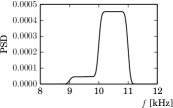
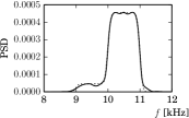
To discuss the approach, it is worth considering an example. Assume that the goal PSD is as shown in Fig. 2a. This is obtained from a function returning $1$ for $f\in[9,10]\,\mathrm{kHz}$, $10$ for $f\in[10,11]\,\mathrm{kHz}$ and zero elsewhere. The function is smoothed a little with a non-causal low-pass filter and then scaled to return $\nicefrac{{1}}{{2}}$ as its integral according to the Parseval theorem.

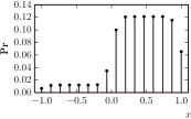
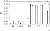
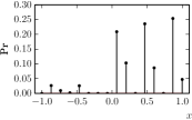
In the proposed experiments, the discrete levels of the modulating PAM signal are assumed to distribute uniformly in $[-1,1]$. Namely, $L_{i}=-1+\nicefrac{{2(i-1)}}{{(N-1)}}$ Fig. 2b shows the reference initial probability vector for $N=16$.

(a)

(b)

Figure 2: Sample goal PSD LABEL:sub@sfig:goal1 and corresponding reference initial probability vector LABEL:sub@sfig:initial1 for $N=16$.

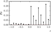
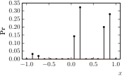
To begin with, some experiment can be run fixing $m$ (preventing the optimizer from changing it) and merely perturbing the initial probability vector with respect to the reference one. In this setup, changing the initial probability vector can in some cases change the optimal solutions being found. However, all the so found solutions tend to have very little differences in cost. Furthermore, the achieved $P_{i}$ values end up being relatively similar among different solutions, namely, those values that are large in one solution remain large in another. Even if experimental tests cannot provide definitive answers, one can thus conjecture that at fixed $m$, either there are no local minima (and the observed one are artifacts from finite machine precision) or they are rather close to each other. As an example, of the few experienced cases where randomizing the initial condition has resulted in slightly different solutions is shown in Fig. 3, which refers to $m=2$.

(a)

(b)

(c)

(d)

Figure 3: Optimal $P_{i}$ (left column) and corresponding PSD (right) when practicing optimization at fixed $m=2$, with $N=16$. In LABEL:sub@sfig:prob1.m2.ref and LABEL:sub@sfig:psd1.m2.ref the reference initial vector is adopted. The corresponding $\nu$ is $0.0182$. In LABEL:sub@sfig:prob1.m2.rnd1 and LABEL:sub@sfig:psd1.m2.rnd1, a random initial vector is used. $\nu$ is $0.0171$.

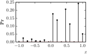
The situation is much more interesting when the optimizer is allowed to choose $m$ too. In this case, the initial $m$ appears to be a strong selector for the final solution. Unfortunately, at least starting from the reference probability vector, it is impossible to partition $\mathbb{R}^{+}$ in simple regions of convergence. In other words, it is impossible to identify intervals of $m$ values such as the optimizer always converges to an optimal $m$ inside them. Still, in general, starting at a large $m$ tends to return a large $m$ solution and viceversa. Some examples are shown in Fig. 4.

(a)

(b)

(c)

(d)

(e)

(f)

(g)

(h)

(i)

(j)

Figure 4: Some local optima. In LABEL:sub@sfig:prob1.ms6.ref and LABEL:sub@sfig:psd1.ms6.ref, $m=5.72$ and $\nu=0.0146$. In LABEL:sub@sfig:prob1.ms4.ref and LABEL:sub@sfig:psd1.ms4.ref, $m=3.79$ and $\nu=0.0109$. In LABEL:sub@sfig:prob1.ms3.ref and LABEL:sub@sfig:psd1.ms3.ref, $m=2.86$ and $\nu=0.0102$. In LABEL:sub@sfig:prob1.ms1-5.ref and LABEL:sub@sfig:psd1.ms1-5.ref, $m=1.93$ and $\nu=0.0149$. In LABEL:sub@sfig:prob1.ms0-2.ref and LABEL:sub@sfig:psd1.ms0-2.ref, $m=0.99$ and $\nu=0.0157$.

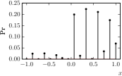
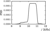
As it can be seen, even with discrete tones one can approximate a given PSD with extremely good accuracy. For instance, this is the case for the $m=2.86$ solution where the cost is $0.0102$. Even more interestingly, good approximations can be obtained even at rather small $m$. For instance, it is possible to follow relatively well the rapid variation of $\bar{\Phi}_{ss}(f)$ around 10 kHz even at $m\approx 1$, as shown in Fig. 4j.

An appealing result of the optimization is that local optima corresponding to low $m$ values have many tones silenced. With this, the CE-SS signal can be eventually generated out of a very little number of frequencies. For instance, in the sample case, at $m=0.99$, only 6 tones are used, out of the 16 initially available.

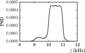
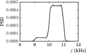
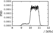
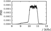
To show that the approach actually works even when tested for relatively short signal chunks, Fig. 5 shows the PSDs of two CE-SS signals generated with the proposed approach and corresponding to the local minima at $m=3.79$ and $m=0.99$. Spectral estimation is practiced by the Welch method operating on signal chunks 16 s long. For the estimation the signals are sampled at $3.79\,\mathrm{\mu s}$ and the Welch algorithm is tuned to use windows of 32768 samples. Conformance to the expected PSD is almost perfect in both cases.

(a)

(b)

Figure 5: PSDs obtained from time domain simulations. In LABEL:sub@sfig:welch4, PSD of a CE-SS signal obtained with the probability vector in 4c and with $m=3.79$. In LABEL:sub@sfig:welch0-2, the probability vector is that in 4i and $m=0.99$.

V Conclusions

In this work, an optimization based strategy to synthesize CE-SS signals with preassigned spectrum by frequency hopping through limited sets of available tones has been presented. The approach relies on nonlinear optimization and has been tested with the SLSQP nonlinear optimizer. The approach can deliver good approximations of the target spectrum, both for the example case discussed in the paper and for many other that have been tried but could not be reported. The optimization problem has multiple local minima that do not represent a significant issue since they can be scanned by selecting different initial values for the modulation index. Quite interestingly, at fast modulations the number of tones required for the approximation can turn out to be much lower than expected.

References

- [1] R. A. Scholtz, “The origin of spread spectrum,” IEEE Transactions on Communications, pp. 822–854, May 1982.
- [2] C.-Y. Pan and C. Kwang-Ting, “Pseudorandom testing for mixed-signal circuits,” IEEE Trans. Comput.-Aided Design Integr. Circuits Syst., vol. 16, no. 10, pp. 1173–1185, Oct. 1997.
- [3] M. Negreiros, L. Carro, and A. A. Susin, “Low cost analogue testing of RF signal paths,” in Proc. of the Design, Automation and Test in Europe Conference (DATE), vol. 1, Feb. 2004, pp. 292–297.
- [4] S. Callegari, F. Pareschi, G. Setti, and M. Soma, “Complex oscillation based test and its application to analog filters,” IEEE Trans. Circuits Syst. I, vol. 57, no. 5, pp. 956–969, May 2010.
- [5] K. B. Hardin, J. T. Fessler, and D. R. Bush, “Spread spectrum clock generation for the reduction of radiated emissions,” in Proceedings of the International Symposium on Electromagnetic Compatibility, 1994, pp. 227 –231.
- [6] M. Balestra, A. Bellini, C. Callegari, R. Rovatti, and G. Setti, “Chaos-based generation of PWM-like signals for low-EMI induction motor drives: Analysis and experimental results,” IEICE Transactions on Electronics, vol. E87-C, no. 1, pp. 66–75, Jan. 2004.
- [7] A. T. K. Tang, “Bandpass spread spectrum clocking for reduced clock spurs in autozeroed amplifiers,” in Proc. of ISCAS’01, Sydney (AU), 2001.
- [8] T. H. Gan, D. A. Hutchins, D. R. Billson, and S. D. W., “The use of broadband acoustic transducers and pulse-compression techniques for air-coupled ultrasonic imaging,” Ultrasonics, vol. 39, no. 3, pp. 181 – 194, 2001.
- [9] M. P. Kennedy, R. Rovatti, and G. Setti, Eds., Chaotic Electronics in Telecommunications. Boca Raton, USA: CRC International Press, 2000.
- [10] S. Callegari, M. Ricci, S. Caporale, M. Monticelli, M. Eroli, L. Senni, R. Rovatti, G. Setti, and P. Burrascano, “From chirps to random-FM excitations in pulse compression ultrasound systems,” in Proceedings of IUS, Dresden (DE), Oct. 2012, pp. 471–474.
- [11] F. Pareschi, G. Setti, S. Callegari, and R. Rovatti, “Implementation of low EMI spread spectrum clock generators exploiting a chaos-based jitter,” in Intelligent Computing Based on Chaos, L. Kocarev, Z. Galias, and S. Lian, Eds. Berlin: Springer, 2009, ch. 7, pp. 145–171.
- [12] S. Callegari, R. Rovatti, and G. Setti, “Spectral properties of chaos-based FM signals: Theory and simulation results,” IEEE Trans. Circuits Syst. I, vol. 50, no. 1, pp. 3–15, Jan. 2003.
- [13] ——, “Chaotic modulations can outperform random ones in EMI reduction tasks,” Electronics Letters, vol. 38, no. 12, pp. 543–544, Jun. 2002.
- [14] S. Callegari, “Generation of band-pass constant-envelope signals with a pre-assigned spectrum: a synthesis procedure,” International Journal of Circuit Theory and Applications, vol. 30, no. 5, pp. 481–486, Sep. 2002.
- [15] D. Kraft, “Algorithm 733: TOMP–fortran modules for optimal control calculations,” ACM Transactions on Mathematical Software, vol. 20, no. 3, pp. 262–281, 1994.
- [16] R. Piessens, E. de Doncker-Kapenga, C. W. Überhuber, and D. K. Kahaner, Quadpack A Subroutine Package for Automatic Integration. Berlin: Springer Verlag, 1983.