Precise time-series photometry for the Kepler-2.0 mission

Abstract

The recently approved NASA K2 mission has the potential to multiply by an order of magnitude the number of short-period transiting planets found by Kepler around bright and low-mass stars, and to revolutionise our understanding of stellar variability in open clusters. However, the data processing is made more challenging by the reduced pointing accuracy of the satellite, which has only two functioning reaction wheels. We present a new method to extract precise light curves from K2 data, combining list-driven, soft-edged aperture photometry with a star-by-star correction of systematic effects associated with the drift in the roll-angle of the satellite about its boresight. The systematics are modelled simultaneously with the stars’ intrinsic variability using a semi-parametric Gaussian process model. We test this method on a week of data collected during an engineering test in January 2014, perform checks to verify that our method does not alter intrinsic variability signals, and compute the precision as a function of magnitude on long-cadence (30-min) and planetary transit (2.5-hour) timescales. In both cases, we reach photometric precisions close to the precision reached during the nominal Kepler mission for stars fainter than $12^{\rm th}$ magnitude, and between 40 and 80 parts per million for brighter stars. These results confirm the bright prospects for planet detection and characterisation, asteroseismology and stellar variability studies with K2. Finally, we perform a basic transit search on the light curves, detecting 2 bona fide transit-like events, 7 detached eclipsing binaries and 13 classical variables.

1 Introduction

The NASA Kepler mission, launched in 2009, collected wide-field photometric observations of over 150 000 stars located in a single, 110-sq. deg. field of view (FOV) continuously over 4 years. The unprecedented precision, baseline and homogeneous nature of this dataset has revolutionised the fields of exoplanet and stellar astrophysics. The analysis of the first 22 months of data alone has led to the detection of thousands of planet candidates, ranging from super-Jupiter to sub-Earth size, including some located in the habitable zone of their host stars (Borucki et al., 011a, 011b; Batalha et al., 2013; Burke et al., 2014), and the analysis of the full 4-year dataset is still underway. However, the failure of the second of four reaction wheels in 2013 forced the nominal mission, which relied on exquisite pointing control, to end prematurely. After a period of tests to evaluate the pointing performance and photometric precision achievable with only two reaction wheels, the satellite has now embarked upon a new mission, called Kepler-2.0, or K2. Over the next 2–3 years, K2 will observe 4 fields per year for $\sim 80$ days each. As the two remaining reaction wheels control the pitch and yaw, the thrusters must be used to alter the roll angle of the spacecraft about its boresight. The K2 fields are thus located in or near the orbital plane of the spacecraft (which is approximately in the Ecliptic plane) so as to minimize the torque induced by solar pressure about the boresight of the telescope. The thrusters are fired every few hours to correct the roll angle to its nominal value.

The science goals, observing strategy and preliminary performance of the K2 mission are described in Howell et al. (2014, hereafter H14). Briefly, the top-level science goals include:

• the search for planetary transits around bright $R\leq 12$ Sun-like stars and around low-mass (late K and early M) stars (K2 will observe roughly as many of these in each pointing as Kepler did in its entire lifetime);

• the search for transiting planets around, and other forms of variability in, tens of thousands of stars in a wide range of Galactic environments (compared to the single direction observed by Kepler);

• observations of nearby open clusters and star forming regions, including asteroseismology, rotation and activity studies, and searches for eclipsing binaries and transiting planets;

• observations of a wide range of extragalactic sources including supernovae.

Aside from the different pointing strategy, K2 will be operated in a similar way to Kepler. Small ‘postage stamps’ will be extracted from the raw images around each target of interest, and co-added on board to result in a cadence of 29.4 min (long-cadence) for most stars, before downlinking to the ground. A small subset of the targets will be observed in short (1 min) cadence mode. Owing to the reduced pointing accuracy, the postage stamps collected have to be larger than during the nominal Kepler mission, so the total number of targets observed per field is much smaller (10–20 000 per run, compared to $\sim$160 000 for Kepler). Beyond this there are two important differences in the way targets are selected for observation and the way the data is processed. The targets for each run are proposed by the community at large and allocated on the basis a ranking of their scientific value. Where a large number of targets are proposed in a relatively small area of sky (e.g. in an open cluster), multiple postage stamps can be collected together to form a so-called ‘superstamp’. Additionally, for the first year of operations at least, the data will be released to the community in the form of target pixel files (TPFs) rather than light curves. TPFs are sequences of postage stamp images calibrated for known, pixel-level effects using the first stages of the Kepler data processing pipeline.

The rest of the pipeline used during the nominal Kepler mission to extract light curves and correct them for instrumental systematics, as well as to search for and validate planetary transits, will need some modifications before they can be applied to K2. In the mean time, the community is being encouraged to develop and use alternative light curve extraction and calibration methods, applying them to the TPFs which will be released approximately 6 weeks after the end of each K2 observing run. The present paper presents one such method, a purpose-written pipeline designed to extract light curves from K2 photometry and correct them for systematic effects associated with the pointing drift of the satellite.

To develop and test our method, we used the so-called two wheel engineering test dataset, which was recently released by the K2 science office for this purpose. This dataset consists of 2079 long-cadence and 18 short-cadence TPFs, each containing $50\times 50$ pixel postage stamps, collected over a period of 9 days, corresponding to 440 long-cadence and 13200 short-cadence observations. The TPFs were created from the data downloaded from the spacecraft by the Kepler pipeline (Jenkins et al., 2010). The present paper focusses on the long-cadence observations (our method can be extended to short-cadence data, but this is deferred to a later paper). While most TPFs were centred on a specific star, two ‘superstamps’ were created using blocks of contiguous TPFs, one near the centre of the FOV and one near the edge. The first $\sim 2.5$ days of data were collected in coarse pointing mode (i.e. using external star trackers to control the spacecraft pointing) and the remainder in fine pointing mode (i.e. using the fine guidance sensors mounted on the focal plane to control the pointing).

The paper is structured as follows: the methods used to extract the photometry and calibrate the systematics are presented in Sections 2 and 3, respectively. The results are discussed in Section 4, where we evaluate the photometric precision of the light curves as a function of magnitude, and discuss the behaviour for variable stars. In Section 5 we compare the performance of our pipeline to other published methods for extracting photometry for K2, and carry out a transit search on stars brighter than $14^{\rm th}$ magnitude. Finally, Section 6 summarises our results and their implications for the K2 key science goals, and outlines areas for future work.

2 Light curve extraction

2.1 List-driven aperture photometry

The approach we adopt to extract photometry from the K2 TPFs is based on experience gained in the context of several ground-based wide-field time-series photometric surveys, namely: the Monitor project (Aigrain et al., 2007), the UKIRT WFCAM Transit Survey (WTS, Nefs et al. 2012), and the VISTA variables in the Vía Láctea survey (VVV, Saito et al. 2012). In all of these, we obtained the most satisfactory results in terms of photometric precision using list-driven aperture photometry, which consists of:

1. running source detection software to identify the sources in each image or frame, and measuring their centroid positions. This results in a catalog of sources for each image.

2. deriving a precise astrometric solution by comparing the catalogs extracted from each image to a master catalog, which can be constructed from a master image (e.g. a stack of a subset of the images taken in the best conditions, if extracting faint sources is important) or a publicly available catalog.

3. performing soft-edged aperture photometry on each frame for each source in the master catalog, by placing a circular aperture at the location of the source on that image, as computed from its sky coordinates (more details on the aperture photometry are given below).

We attribute the success of this method so far to its relative simplicity, and to the fact that the global astrometric solution used is much more precise than the individual centroid position measurements for each star, particularly for fainter stars (typical uncertainties in the astrometric solution for Nyquist-sampled images are of order 0.1 pixels).

The basic aperture function used is a circular top hat with no tapering. Flux from pixels completely enclosed within the aperture boundary are given full weight ($w_{i}=1$). The soft-edging refers to those pixels intersected by the boundary. For these the background-corrected flux $f_{i}$ is split pro-rata according to the fractional area $w_{i}$ of the pixel enclosed within the boundary. For an isolated image, this is simply equivalent to defining the total flux as $\sum_{i}f_{i}\times w_{i}$. For overlapping or blended images, we treat the circular top-hat as a point-spread function (PSF) and do simultaneous PSF fitting using the same pro-rata split to define the individual model PSFs across boundaries.

Although circular apertures/PSFs are not optimal for all images, they are close to optimal for cases where the Poisson noise from the objects is the dominant noise contributor. They also have the advantage of minimising the impact of systematics caused by uncertainties, or any mismatch, in the exact shape of the PSF. For example, conventional weighted PSF fitting introduces a magnitude-dependent systematic offset between total flux and PSF-derived flux in such cases which is absent in our aperture-based approach.

2.2 Implementation for K2

To apply this method to K2 data, we must first construct full frame images (FFIs) from the K2 TPFs. To do this, we start from a Kepler FFI (taken during the nominal mission). Kepler FFIs are multi-extension FITS files with 4 extensions for each of the 21 science modules (each module consists of 2 $1048\times 1048$ pixel CCDs, each of which is divided into 2 output channels). For each K2 long-cadence observation, a new copy of the original Kepler FFI is created, and all the image arrays are set to zero. For each TPF, the postage stamp image corresponding to this observation is then inserted at the appropriate location in the relevant extension (using the meta-data contained in the TPF headers). For each extension, we also used the python module k2fov to compute the sky coordinates of the 4 corners of each output channel, and from these we obtained a first estimate the crval and cdx_x header keywords describing the World Coordinate System (WCS) solution, which were inserted in the extension header. We also generated a single binary mask with the same format as the FFIs, which is 1 where there is data and 0 where there is none. We used this mask as a confidence map, and note that it could be refined further to flag bad pixels and account for effects such as vignetting over the field of view, if needed.

We then performed source extraction, astrometric solution and list-driven aperture photometry on the FFIs using the imcore, wcsfit and imcore-list routines from the casutools package (Irwin et al., 2004), using our binary mask as a confidence map. Note that the confidence map could also be used to flag bad pixels and account for effects such as vignetting over the field of view, if needed. The source extraction software normally makes a local estimate of the background at each point in the image using the median of a $64\times 64$-pixel window, which is larger than the K2 postage stamps; we therefore proceed using a single, global background estimate for each extension, but bearing in mind a more careful background correction may be needed at a later stage. For example, this could be done by fitting a simple surface to the background variation over each detector or output channel (the latter might be needed if differences in bias correction between channels corresponding to the same detector).

The astrometric solution was obtained relative to the 2MASS all-sky point-source catalog, using the catalog extracted from the first image as the master catalog. This resulted in a total of 13 977 sources, of which 13 633 were detected (at the 4-$\sigma$-level on $>50\%$ of the images. The typical root mean square (RMS) of the astrometric solution was 0.4″, or approximately 0.1 pixel, which is satisfactory given the under-sampled nature of the Kepler point-spread function (PSF).

The pipeline evaluates the flux of each source on each image by placing a circular aperture centred at exactly the same sky position on every frame, derived from the global astrometric solution. In our experience, this approach gives systematically better results than using the centroid or best-fit position of each source as measured on each frame to locate the aperture. Our apertures are soft-edged, in the sense that pixels straddling the edge of the aperture contribute partially to the flux, as opposed to the pixellated masks used by the Kepler pipeline. Finally, the pipeline automatically deblends sources with overlapping apertures, assigning the appropriate fraction of the flux in the overlap pixels to each aperture by simultaneously fitting a ‘top hat’ function to all overlapping sources in a blend.

Aperture radii:

We computed fluxes using 6 different aperture radii: 1.5, 3, $3\sqrt{2}$, 6, $6\sqrt{2}$ and 12 pixels. In general, larger apertures are more suitable for brighter sources, as the flux in the wings of the PSF remains significantly above the background out to larger radii. The optimal aperture radius to use for a given star also depends on its individual neighbourhood: if a source has a close neighbour, a very small aperture which excludes as much of the neighbour’s flux as possible or a very large one which encompasses both sources might give better results than an aperture of intermediate size. However, different apertures can be more or less sensitive to certain systematic effects, and yield better performance depending on the main timescales of interest. We therefore process all the aperture fluxes in parallel for every star. Throughout the paper, we use the 3-pixel apertures, unless stated otherwise. This radius corresponds to approximately twice the full-width at half-maximum (FWHM) of the PSF, which in our experience gives good results for most sources across a wide range of magnitudes, although one should bear in mind that it may not be optimal at either end of the magnitude range. We return to the question of how to select the aperture radius more in Section 4.4.

2.3 Catalog cross-matching and zero-point calibration

In order to be able to identify known variables among our sources, and to be able to place the objects on a standard magnitude scale, we cross-matched the list of objects for which we extracted light curves (our master catalog) with the target list supplied with the test dataset (hereafter, the input target list). This was done by locating, for each object in the latter, the closest positional match in the former. For 56 of the 1951 targets in the input target list, the closest match in the master catalog was located further than 8″away, i.e. approximately two Kepler pixels. Some of these could be faint objects which were not detected by our source detection software, but a number are relatively bright. These could be high proper motion objects where the the nominal position in the input target list does not match the actual position at the time of the observations.

We then calibrated the flux measurements obtained using each aperture radius onto the Kepler magnitude scale by fitting, for all the matches closer than 8″, a relation of the form:

$$K_{\rm p}={\rm zp}_{X}-2.5\log({\rm flux}_{X})$$

where $K_{\rm p}$ is the Kepler magnitude and the subscript $X$ refers to the different aperture radii. The zero points obtained in this way were all between 25 and 25.3 (for fluxes expressed in e^-/s). For faint objects with nearby neighbours, the magnitude is strongly dependent on the aperture size used. Therefore, for the remainder of this paper, we adopt a single magnitude for each object, based on the 3-pixel aperture fluxes.

We checked if there were any trends in the flux versus magnitude relation depending on the distance of the source from the satellite boresight. Such a trend might be expected due to the fact that the images of stars located near the corners of the FOV are significantly elongated, which could cause some of the flux to fall outside the aperture, but we found no evidence for it.

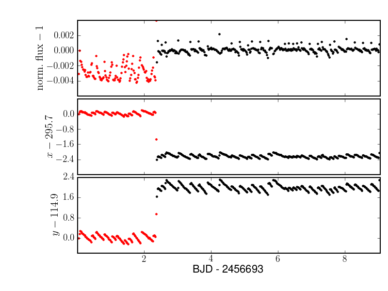
Figure 1: Example raw light curve and centroid coordinates (EPIC no. 60021515, cool dwarf, Kepler magnitude $K_{\rm p}=11.3$, located in module 9, output channel 1). Data taken before fine-pointing was achieved are shown in red.

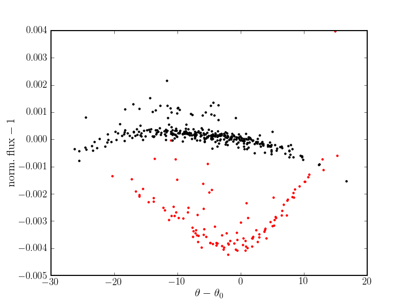
Figure 2: Same as Figure 1, but now showing flux versus the roll angle $\theta$ of the spacecraft. Here $\theta$ is the mean of the roll angle estimates derived from the astrometric solution for each channel, relative to a reference frame (which is simply the first frame in the dataset). Note the tight but nonlinear relationship between flux and roll angle, which differs before and after fine-pointing was achieved, as the star is located on a different set of pixels.

2.4 Raw light curves

Figure 1 shows an example light curve resulting from the procedure described in the previous section. Most light curves show significant variations of instrumental origin, which are clearly correlated with the object’s position on the detector. These variations, which presumably are due to a combination of intra-pixel and inter-pixel (flat-field) sensitivity variations, must be corrected before the light curves become astrophysically useful.

The pitch and yaw of the spacecraft are fairly stable, as they are controlled by the two remaining functioning reaction wheels. However, the roll about the boresight displays a gradual drift due to the Sun’s radiation pressure, and is reset approximately every 6 hours using the spacecraft’s thrusters. This causes the star to wander over the detector by a significant fraction of a pixel, and leads to systematic variations in the measured flux. Indeed, as shown in Figure 2, the systematic flux variations are tightly correlated with the roll angle (they also show a correlation with the star’s individual $x$- and $y$-position, but less tight). Note that we estimated the roll angle in each frame for each output channel from the crval parameters of the astrometric solution, and then adopted the median of the individual channel values as our global roll angle estimate.

3 Systematics correction

We experimented with a number of established methods for modelling these roll-dependent systematic effects, starting with simple linear decorrelation of the flux against roll angle, or the $x$- and $y$- coordinates of the star’s centroid as measured on each image. We also tried using the well-known SysRem algorithm (Tamuz et al., 2005), where the systematic trends are iteratively identified as the first principal component of the matrix constructed from all the light curves, and each trend is removed by linearly decorrelating the flux measurement for each star against it. The systematics correction in the PDC-MAP pipeline used during the nominal Kepler mission (Smith et al., 2012) is a variant on this approach, where a Bayesian framework is used to ensure that the coefficients relating each star’s light curve to each trend are similar for stars of similar magnitude and position on the detector, as might be expected is their physical origins are similar. However, no PDC-MAP data are publicly available at the time of writing for this dataset. Finally, we also tested the ‘Astrophysically Robust Correction’ (ARC) method proposed by Roberts et al. (2013), once more in the context of the nominal Kepler mission. This is again a variant on SysRem-like approaches, where additional measures are used at the trend detection and removal stages to minimize the risk of removing variability of astrophysical origin. However, none of these approaches gave satisfactory results: in some light curves the systematics were only partially corrected, while in others systematics were actually introduced by the correction.

3.1 Gaussian process model

All of the methods described above implicitly assume that the relationship between the trends and the stellar fluxes is linear, and this is not generally the case for K2 data, as can be seen in Figure 2. In fact, while flux is often correlated with roll angle, the amplitude and shape of the relationship between the two varies from star to star, even for stars of similar brightness located close to each other on the detector. This is because inter- and intra-pixel sensitivity variations (flat-field) are the dominant source of systematics for K2. The exact manner in which the roll angle variations impact the star’s measured flux depends on the response of the specific set of pixels on which each star falls.

Systematics removal approaches based on linear basis modelling can be used to remove non-linear effects, so long as the behaviour can be described by a linear combination of such models and the driving systematic variables can be identified. However, we do not know a priori whether these conditions apply for the present dataset. We therefore opted to model the systematics using a Gaussian Process (GP) with roll angle as the input variable. This approach assumes that the systematics are related to the roll angle variations, but makes no assumptions about the functional form of that dependence: instead it marginalises over all possible functions, subject to certain smoothness constraints. Each star is modelled individually, so the functional form of the systematics is allowed to vary from star to star. This also enables us to model the intrinsic variability of each star at the same time as we fit for the systematics model, in an effort to minimize the extent to which the systematics correction interferes with the real astrophysical signals.

We omit here a detailed explanation of GP regression, as many are available elsewhere. For example, the interested reader will find a thorough, textbook-level introduction to GPs in Rasmussen & Williams (2006), or a more succinct introduction in the context of modelling systematics in high-precision stellar photometry in Gibson et al. (2012). For our purposes, a GP can be thought of as setting up a probability distribution over functions, whose properties are constrained by parametrising the covariance between pairs of observations. Specifically, we postulate that pairs of flux measurements taken at similar values of the roll angle (i.e. when the star fell at approximately the same position on the detector) should be strongly correlated, while pairs of flux measurements taken at very different values of the roll angle should be essentially uncorrelated. This is expressed mathematically by the covariance function, or kernel:

$$k_{\theta}(\theta_{i},\theta_{j})=A^{2}_{\theta}\exp\left[-\frac{|\theta_{i}-\theta_{j}|^{2}}{2L^{2}_{\theta}}\right]$$

This form of kernel, known as a squared exponential (SE), is one of the most commonly used, and gives rise to smooth variations which a characteristic length scale $L_{\theta}$ and amplitude $A_{\theta}$. The likelihood of observing a sequence of $N$ flux measurements $\mathbf{y}\equiv\{y_{1},y_{2},\ldots,y_{N}\}$ is then a multivariate Gaussian:

$$\mathbf{y}\sim\mathcal{N}(\mathbf{0};\mathbf{K}),$$

where the mean of the distribution has been set to zero, and the individual elements of the covariance matrix $\mathbf{K}$ are given by the kernel for the corresponding inputs. Note that we work with light curves that have been normalised by subtracting their median and dividing them by a robust estimate of their scatter, estimated as $\sigma_{\rm MAD}=1.48\,{\rm MAD}$, where ${\rm MAD}$ is the median of the absolute deviation from the median.

In practice, the measured flux does not depend on roll angle alone: the light curve also contains intrinsic variations of astrophysical origin, which depend on time, and observational (white) noise. We therefore adopt a composite kernel function of the form

$$k(\{t_{i},\theta_{i}\},\{t_{j},\theta_{j}\})=k_{t}(t_{i},t_{j})+k_{\theta}(\theta_{i},\theta_{j})+\sigma^{2}\delta_{ij},$$

where

$$k_{t}(t_{i},t_{j})=A^{2}_{t}\exp\left[-\frac{|t_{i}-t_{j}|^{2}}{2L^{2}_{t}}\right]$$

represents the intrinsic variations, $\sigma^{2}$ is the white noise variance and $\delta$ is the Kronecker delta function. The additive form of the adopted kernel enables us to separate the different contributions from roll angle, time, and white noise. The use of an SE kernel with a single length scale and amplitude to model the intrinsic variability of each star, which can be quite complex, is an oversimplification, but it is sufficient for the purpose at hand, which is merely to help disentangle between intrinsic and instrumental variations.

3.2 Implementation for this dataset

As shown on Figures 1 and 2, the data collected in coarse pointing mode present larger roll angle systematics, with a different relation between flux and roll angle to that observed for the data collected in fine sampling mode. For the remainder of this paper, we therefore focus only on the data collected in fine pointing mode. However, we note that the same procedure could be applied separately to the data collected in coarse pointing mode, though the time-dependent component of the GP would not be well-constrained given the short duration of that data segment.

3.3 Initial guesses, parameter optimisation and outlier rejection

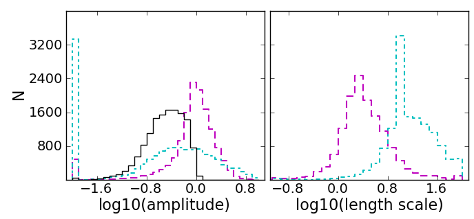
Figure 3: Histogram of the best-fit GP amplitude and length scale parameters (left and right panels, respectively). The amplitudes are relative to the scatter of the original (uncorrected) light curve. The dashed magenta, dash-dot cyan and solid black lines correspond to the time, roll angle and white noise components, respectively.

For each light curve, we start with a prior for the covariance parameters $\{A_{t},\,L_{t},\,A_{\theta},\,L_{\theta},\,\sigma\}$ which, after visual inspection of several tens of randomly selected light curves, was set to $\{0.5,2\,{\rm days},\,0.2,\,10\,{\rm arcsec},\,0.2\}$. These values give an adequate description of most light curves, though they are not suitable for the final correction. We then evaluate the mean and variance of the predictive distribution of the GP conditioned on the data, initially without adjusting the covariance parameters. Any data points lying further than $3\,\sigma$ from the predictive mean are flagged as likely outliers. This step is necessary as most light curves contain a number of outliers can otherwise significantly affect the determination of the best-fit covariance parameters. We have not established the precise origin of these outliers, but they tend to occur near the times where the roll angle of the satellite was reset using the thrusters. Such a manoeuvre could cause certain parts of the detector to heat up, and/or smear the stellar flux over a larger area, both of which could lead to an anomalous flux measurement for the corresponding cadence.

We then optimize the likelihood with respect to the covariance parameters using a standard local optimisation algorithm within pre-set bounds (specifically, the scipy implementation of the L-BGFS-B algorithm by Byrd et al. 1995), and ignoring the outliers flagged at the previous step. The amplitudes were constrained to be $>0.01$ and the length scales were constrained to lie in the range 0.1–100. Fig. 3 shows histograms of the resulting best-fit GP parameters. Except for stars which display significant variability on timescales similar to the roll variations (which are discussed in more detail in Section 4.1), the best-fit parameters are insensitive to the initial guesses. We then repeat the outlier flagging procedure, this time using a more stringent threshold of $2.5\,\sigma$, before evaluating the mean of the predictive distribution of the GP a final time. To isolate the component of the flux variations caused by the roll variations, the predictive distribution is evaluated using the actual values of the roll angle, but setting the time to a fixed value (e.g. the middle of the time interval spanned by the observations). This is then subtracted from the original flux measurement, leaving a light curve corrected for roll-dependent systematics.

3.4 Computational cost and subsampling

Fitting for the covariance parameters requires multiple evaluations of the likelihood. For a GP of this type, the computational cost of each likelihood evaluation is $\mathcal{O}(N^{3})$. To speed up the calculation, we subsample the data before fitting for the covariance parameters. For the test dataset, we used every $4^{\rm th}$ data point, which enables each light curve to be processed in 0.5–1 s on a $1.6$ GHz Intel processor without any noticeable effect on the results. More severe subsampling combined with simultaneous processing on multiple cores may be needed for the longer science campaigns.

3.5 Corrected light curves

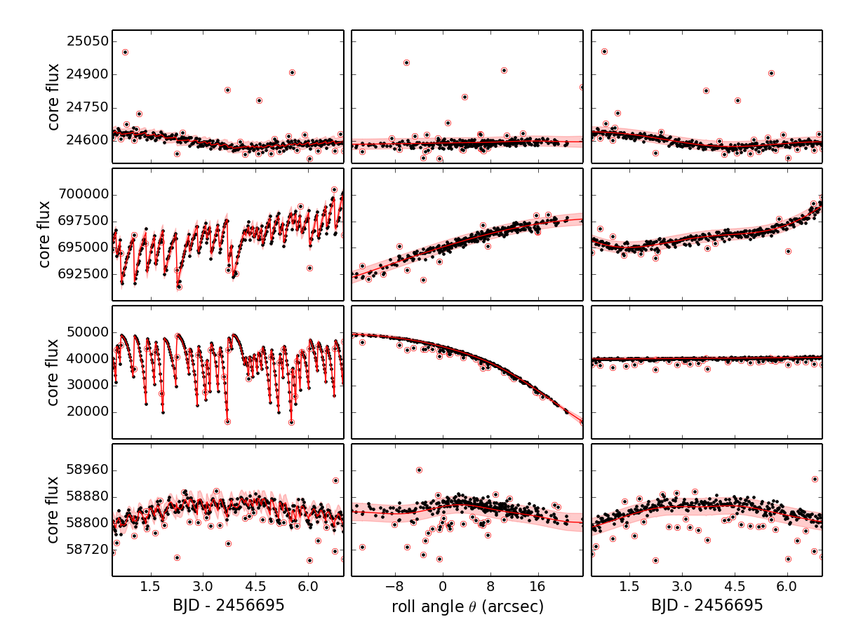
Figure 4: Four examples illustrating the correction of roll-dependent systematics using a GP. In the left column, black dots show the input light curve and the red curve shows the mean of the predictive distribution of the full model (roll-dependent systematics $+$ intrinsic variations). Points falling $>2.5\,\sigma$ away from this line (i.e. outside the pink shaded area) are flagged as outliers and marked by the red circles. The middle column shows flux as a function of roll angle, after subtracting the time-dependent component of the model (i.e. showing only the systematics). Finally, the right column shows the corrected light curve after subtracting the roll-dependent component of the model.

Figure 4 shows four example light curves, before and after correction of the roll-angle systematics. These examples we drawn from a random selection, within which we chose four cases spanning a wide range of magnitudes and locations within the FOV, where the systematics were visible by eye. They include a clearly systematics-dominated case (third row), cases where the systematics have a similar amplitude to the intrinsic (time-dependent) variability (second and fourth row) and a case where both are similar in amplitude to the white noise (top row). We visually examined hundreds of similar examples, and while the systematics are not always strong enough to be noticeable, we found no instance where the correction seemed to introduce spurious effects.

4 Results

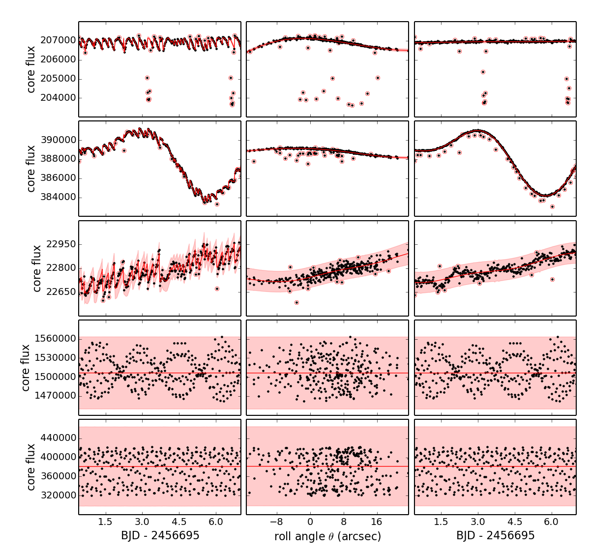
Figure 5: As Figure 4, but now showing selected variable stars. From top to bottom: known transiting exoplanet host star WASP-28 (EPIX 60017806, $K_{\rm p}=12.0$) , a cool dwarf showing slow variations most likely caused by star spots (EPIC 60022118, $K{\rm p}=11.2$), a star displaying low-level stochastic variability (EPIC 60017902, $K_{\rm p}=14.4$), a classical pulsator (EPIC 60018082, $K{\rm p}=9.7$), and a contact eclipsing binary (EPIC 60017809, $K{\rm p}=11.5$). See text for a more detailed discussion.

4.1 Effect on transits and variable stars

Figure 5 illustrates the behaviour of our roll-angle correction for a few selected variable stars.

The top panel shows the known transiting planet host star WASP-28. Our outlier detection procedure flags the in-transit points, and enables the roll-angle correction to proceed using the remaining data. Importantly, while the in-transit points are flagged as outliers, the roll-angle correction is still applied to the full light curve, including the transits. The phase-folded light curve is shown in Figure 6, illustrating the drastic noise reduction brought about by the correction of the roll-angle systematics.

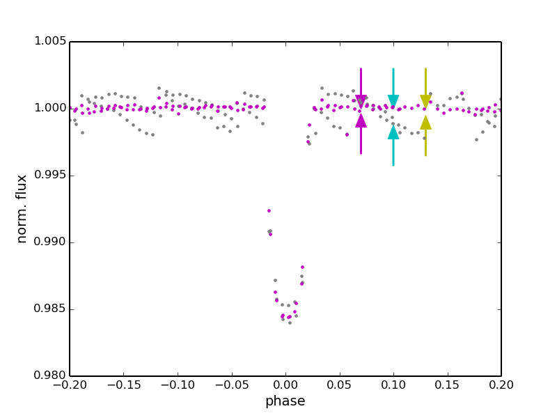
Figure 6: Phase-folded light curve of WASP-28 (using the ephemeris of Anderson et al. 2014). Grey and magenta dots show the raw and roll-corrected data, respectively (long cadence, in both cases). The magenta arrows indicate the depth of a transit that would have been detectable in this light curve with a signal-to-noise ratio of 8 (assuming 3 transits lasting 3 hours each). For comparison, the cyan and yellow arrows indicate the depths of transits caused by a Neptune-sized planet in front of a Sun-like star, and an Earth-sized planet in front of a $0.4\,M_{\odot}$ M-dwarf, respectively.

The second panel shows a cool star displaying smooth variations on timescales of a few days (probably caused by star spots) as well as significant roll-angle systematics. The intrinsic variability is reproduced without difficulty by the time-dependent component of our GP model, enabling the correction of the systematics to proceed unimpeded by the intrinsic variability. This example illustrates the fact that our method is suitable for stellar rotation and activity studies.

The third panel shows a star displaying lower amplitude, more stochastic variability. In this case, only the long-term component of the variability is modelled, and the stochastic behaviour that is not well explained by the roll-angle variation is incorporated in the white noise term. Nonetheless, the roll-angle systematics are corrected successfully, illustrating the fact that our method is suitable for studies of stochastic behaviour such as accretion related variability in young stars.

The last two panels show stars displaying periodic variability on timescales very similar to the roll angle variations (a pulsating star and a contact eclipsing binary, respectively). In those cases, our model does not reproduce the variability, and neither does it identify (and hence correct) any roll-angle systematics. The amplitude of the time and roll-angle terms becomes negligible, while the white noise term becomes anomalously large. These objects are easy to identify (in Figure 3, they fall in the lowest time and roll-angle amplitude bins and in the highest white noise amplitude bin). Furthermore, they are not pathological, as the light curve is unchanged by the correction, so no spurious effects are introduced. Nonetheless, anyone interested in studying this specific type of object at very high precision would need to develop a different approach to identify and remove roll-angle systematics. One way of doing this might be to model the periodic variability explicitly (using a sum of sinusoidal terms), simultaneously with the roll-angle systematics (using a GP). Alternatively, phase dispersion minimisation (PDM, Stellingwerf 1978) could be used to remove the periodic variability without explicitly modelling it, before correcting the for the roll angle systematics, and then adding the periodic component back onto the residuals.

4.2 Photometric precision

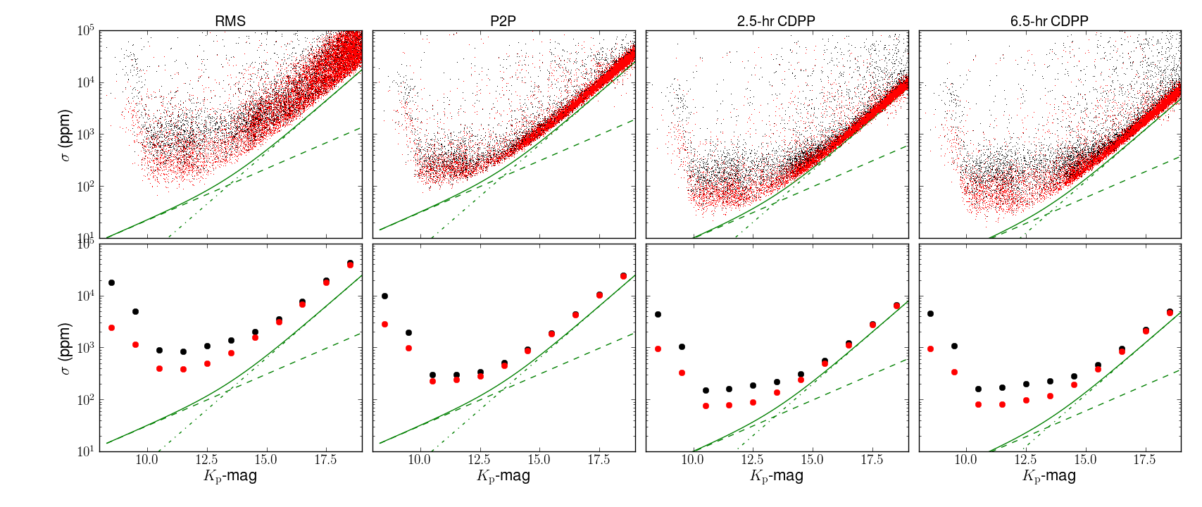
Figure 7: Relative photometric precision (in parts per million) as a function of magnitude, before (black) and after (red) correction of the roll-angle systematics, using 3-pixel apertures. From left to right: full light curve scatter, point-to-point scatter, 2.5-hour and 6.5-hour quasi-CDPP (see text for details). The top panel shows all objects, while the bottom shows the median values in 1-mag bins. The green solid, dashed and dash-dot lines show the theoretical total, source, and background $+$ readout noise, respectively.

Mag. range	No. stars	3-pixel apertures				$3\sqrt{2}$-pixel apertures
		RMS	P2P	2.5-hr CDPP	6.5-hr CDPP	RMS	P2P	2.5-hr CDPP	6.5-hr CDPP
9.0–10.0	158	1158	976	331	343	556	249	105	150
10.0–11.0	402	400	227	75	81	340	182	75	113
11.0–12.0	541	383	238	78	80	359	201	74	86
12.0–13.0	366	500	286	90	99	545	279	81	68
13.0–14.0	439	801	452	136	117	1130	516	143	111
14.0–15.0	998	1580	867	242	193	2400	1110	302	231
15.0–16.0	1014	3093	1841	498	383	4922	2544	685	514
16.0–17.0	1403	6896	4230	1121	840	11401	6030	1610	1232
17.0–18.0	2302	17944	10301	2737	2059	28547	13759	3712	2821
18.0–19.0	3578	38752	23673	6304	4713	57747	29125	7770	5856

Table 1: Median photometric precision as a function of Kepler magnitude, in parts per million (ppm), for two aperture sizes.

We evaluated the photometric precision of the light curves using four different metrics. The first is simply the light curve scatter (once again, estimated as $\sigma_{\rm MAD}$) – this is referred to as RMS. The second is the point-to-point scatter, estimated in the same way but from the first difference between consecutive points in the light curve. This estimate, referred to as P2P, includes only the high-frequency component of the noise, multiplied by a factor $\sqrt{2}$. The third and fourth are intended to approximate the combined differential photometric precision (CDPP) used throughout the Kepler mission to quantify the photometric precision on planetary transit time-scales. However, we cannot reproduce the actual CDPP values without access to the transit search component of the Kepler pipeline, since the CDPP is essentially the depth of a transit of a given duration that would give a signal-to-noise ratio of 1 (Christiansen et al., 2012). Instead, we defined a ‘quasi-CDPP’, which we evaluate as the median of the standard deviation of the light curve evaluated in a moving window of a given duration. This procedure is identical to that adopted by Vanderburg & Johnson (2014, hereafter VJ14), the only other study published to date on the photometric precision attainable with this K2. We chose to adopt the same approach to enable us to compare our results directly with theirs, but note that our ‘quasi-CDPP’ estimates are equivalent to the actual CDPP only if the noise is white on the timescale under consideration As the top-level goal of the nominal Kepler mission was the detection of habitable planets, the CDPP was typically measured on 6.5-hour timescales. The limited duration of K2 campaigns (up to 85 days) means that it will be most sensitive to relatively short-period planets with transit durations of 2–3 hours, so we report quasi-CDPP values for both 2.5-hour (5 cadences) and 6.5-hour (13 cadences).

Figure 7 shows these four different estimates of the photometric precision as a function of magnitude before and after correction of the roll-angle systematics, while Figure 8 shows histograms of the relative reduction in these different precision estimates between the original and corrected light curves (for 3-pixel apertures in both cases). Additionally, Table 1 gives the median precision estimates in 1-magnitude bins.

On Fig. 7 we also show the estimated source and background photon noise and readout noise as a function of magnitude, as well as the total theoretical noise estimate obtained by adding them in quadrature. In the left panel, the two contributions were estimated as the square root of the median flux for each source, and the median background flux integrated over the aperture, respectively, after converting the fluxes from e^-/s to e^- by multiplying by the duration of individual on-board exposures (6.02 s) times the number of exposures per cadence (270 for long-cadence data). For the P2P and quasi-CDPP plots, the noise estimates were scaled by a factor $\sqrt{2}$, $1/\sqrt{5}$ and $1/\sqrt{13}$, respectively.

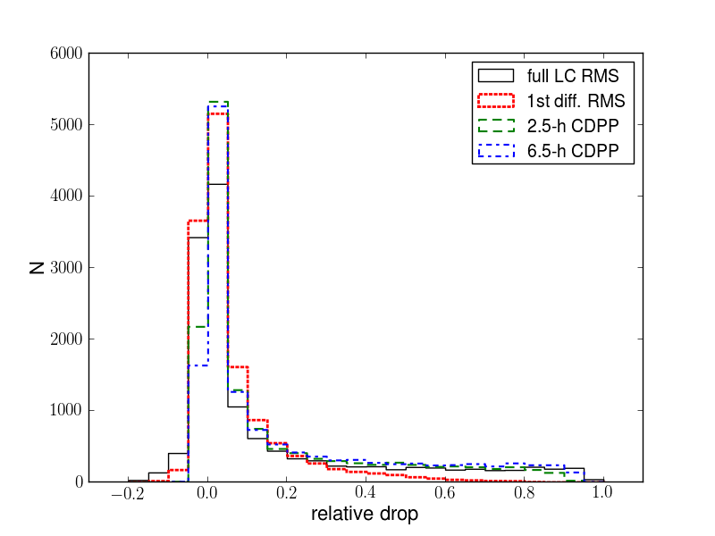
Figure 8: Histogram of the relative reduction in scatter as measured by the full light curve RMS (solid black line), the RMS of the first difference (dotted cyan line) and the 6.5-hour quasi-CDPP (dashed magenta line).

A number of features are worth remarking on. For all metrics used, the lower envelope of the scatter versus magnitude relation corresponds approximately to the photon noise level down to magnitude $K_{\rm p}\sim 15$, and is within a factor 2 of it down to $K_{\rm p}\sim 12$. For brighter stars, the scatter versus magnitude plots flatten off, indicating that an additional source of systematics is present. One possible additional noise source is detector response non-linearity, though using larger apertures for these stars may also help alleviate the problem. The effects of saturation become visible for $K_{\rm p}<10$.

When isolating the scatter on a given timescale, as in the last 3 columns of Fig. 7, the vast majority of stars follow a tight relationship between precision (after correction) and magnitude. This indicates that most of the scatter above this level observed in the raw light curves can be explained by roll-angle systematics. By contrast, the full light curve scatter (RMS) results from the combined effects of intrinsic variability on all timescales, residual instrumental effects and white noise. As a result, a wide range of RMS values are observed for a given magnitude even after correction.

The amount by which the correction reduces the full light curve scatter and the quasi-CDPP varies widely from star to star, ranging from $<10\%$ for most stars, to $>90\%$ for a few hundred cases. These tend to be bright stars displaying little intrinsic variability, or variability on long (days) timescales only, where the systematics were initially dominant. The point-to-point scatter is reduced by a smaller amount, on average, because the dominant timescale of the roll angle variations is significantly longer than the interval between consecutive observations.

4.3 Injection tests

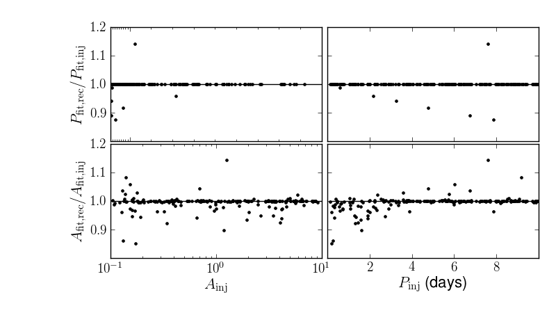
Figure 9: Results of the injection tests (see Section 4.3 for details).

We have already shown qualitatively in Figure 5 that our systematics correction preserves most forms of astrophysical variability. Here we test this in a more quantitative manner by injecting sinusoidal signals into the light curves before correcting them. This test was performed on 200 randomly selected light curves with $10\leq K_{\rm p}\leq 14$, with the default (3-pixel) aperture only. The injected signals had periods drawn from a uniform distribution between 0.1 to 10 days, amplitudes drawn from a log uniform distribution between 0.1 and 10 times the standard deviation of the original light curve, and phases drawn from a uniform distribution between 0 and $2\pi$.

To assess how well the injected signals were preserved, we performed a least-squares fit of a sinusoid to injected and recovered signals, where the recovered signal is defined as the difference between the corrected light curves with and without injected signal. (Note that the amplitude and period of this fit can differ from the injected values, even for the original time-series, owing to the limited duration of the dataset.) The results of the test are shown in Figure 9, which shows the ratio of fitted periods and amplitudes in the original and recovered signals, as a function of the injected amplitude and period. The periods are recovered perfectly (i.e. up to the frequency resolution of the data) in 99.5% of the cases. In the remaining 0.5% of cases, the discrepancy (which nonetheless never exceeds 15%) arises from the fact that the signals were injected into light curves already containing significant variability. As the time-dependent component of our model has a single characteristic time-scale, light curves containing time-variability on multiple, very different timescales can be problematic. The amplitude is recovered to within 1% in 78% of the cases. The amplitude recovery performance is significantly worse for periods $<3$ days, which are more difficult to disentangle from the roll-angle variations, but the amplitude is always recovered to better than 15%. This means that there should be no difficulty in identifying such signals in the detrending light curves, but joint modelling of systematics and astrophysical signals is advisable to obtain accurate amplitudes.

4.4 Aperture selection

As previously mentioned, the best aperture radius to use is expected to decrease with increasing magnitude. Indeed, when we compute the aperture giving the smallest scatter – using any of the 4 metrics described above – for each object individually, the general trend is for smaller apertures for the fainter objects, and larger apertures for the brighter objects. The exact aperture size selected depends on the timescale considered: the P2P, 2.5-hr and 6.5-hr quasi-CDPP statistics favour increasingly larger apertures at a given magnitude. A plausible explanation for this is that the P2P statistic is primarily sensitive to white (background and readout) noise, which is minimized by using smaller apertures, while the quasi-CDPP, particularly on longer timescales, is more sensitive to any residual pointing-related systematics, which are minimised by using slightly larger apertures. This is also visible in Table 1, which lists the median precision metrics in each magnitude bin for two aperture sizes.

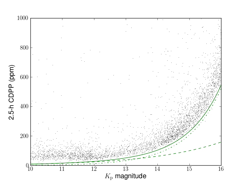
Figure 10: 2.5-hour quasi-CDPP of the light curves corrected for roll-angle systematics, using a magnitude-dependent aperture radius selection. The green solid, dashed and dash-dot lines show the theoretical total, source, and background $+$ readout noise, respectively.

A blind application of the object-by-object aperture selection can have undesirable consequences, however, particularly the faint end, where very large apertures would be selected for a significant fraction of the objects, effectively minimising their scatter by diluting them with the flux of a nearby neighbour. Taking this into account, we ultimately implemented a simplified magnitude aperture selection based on the 2.5-hr quasi-CDPP, but adopting the most commonly selected aperture size in each magnitude bin for all stars in that bin, and enforcing a monotonic increase of aperture size with magnitude. This results in 12-pixel apertures down to $K_{\rm p}=9$, $3\sqrt{2}$-pixel apertures down to $K_{\rm p}=13$, 3-pixel apertures down to $K_{\rm p}=16$, and 1.5-pixel apertures beyond that. Figure 10 shows the resulting 2.5-hr quasi-CDPP as a function of magnitude for $10<K_{\rm p}<16$. This choice of apertures yields performance close to the theoretical noise limit throughout that wavelength range. The use of a small number of fixed aperture sizes introduces ‘jumps’ in precision at the magnitudes where the aperture radius changes, which are visible in Figure 10. These might be avoided by using an aperture radius that varies smoothly with magnitude. However this would require a signficiant re-write of our pipeline, and is therefore deferred to future work.

5 Discussion

5.1 Comparison to other methods

At the time of writing, photometric precision estimates for K2 are available from H14 and (Vanderburg & Johnson 2014, hereafter VJ14).

H14 performed analysed data collected during engineering tests in October 2013 and January 2014 (the latter are the test dataset used in the present paper). Using the publicly available PyKe package developped by the Kepler Guest Observer office, including simple aperture photometry using circular or elliptical apertures and background estimates based on the median of nearby pixels, they achieved a precision on 6-hour timescales of $\sim 80$ ppm for 12^th magnitude G dwarfs, compared to $\sim 20$ ppm for the same stars during the nominal Kepler mission. Overall, they found that the precision over 6-hour timescale was within a factor of 4 of the precision achieved during the nominal Kepler mission.

VJ14 analysed the January 2014 test dataset only, using a purpose written pipeline, which performs simple aperture photometry followed by a correction for systematic effects due to the satellite’s pointing variations on a star-by-star basis. They achieved median photometric precisions (as measured by the 6.5-hour quasi-CDPP) within a factor of 2 of the nominal Kepler performance, a factor of 2 improvement over the preliminary results presented in H14.

Our results are broadly similar to those of VJ14; we obtain slightly better performance for fainter stars, where our results approach the theoretical noise limit, and slightly worse for brighter stars, for which the lower envelope (rather than the median) of our quasi-CDPP distribution is within a factor of 2 of the median Kepler performance (and of the photon-noise limit). This last point may be due to the fact that VJ14 analysed bright stars using very large apertures, whose position was determined by the centroid of each star on each frame. We did try increasing our aperture radius up to 12 pixels, but without significant improvement on the resulting precision.

In principle, our method has several advantages over that of VJ14. It provides light curves for every target on silicon; it should be less sensitive to errors in the measurement of the position of individual stars; the model used for systematics correction is probabilistic, principled, and enables a rigorous propagation of the uncertainties associated with the systematic correction. On the other hand, more work is needed to understand the slightly better performance obtained by VJ14 for bright stars.

5.2 Effect of image distortion across the FOV

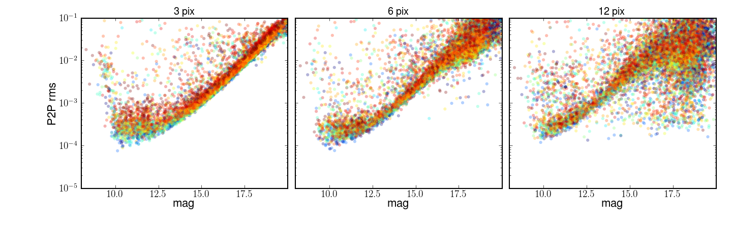
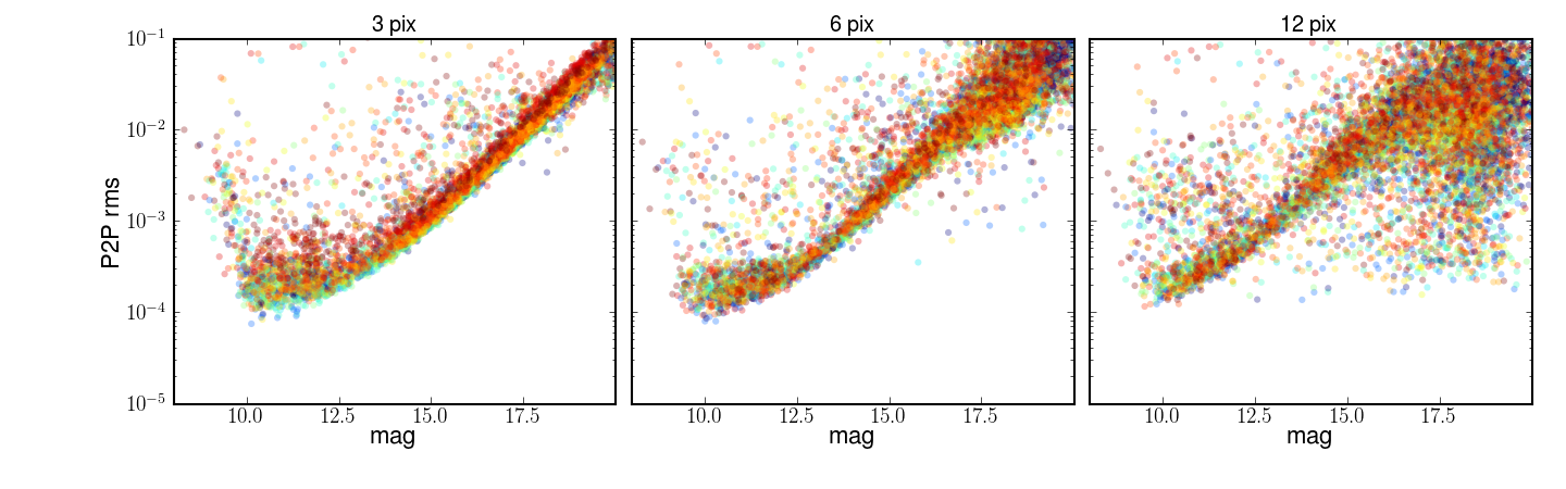
Figure 11: Point-to-point scatter as a function of magnitude using different aperture sizes, colour coded from blue to red according to increasing distance from the centre of the FOV (i.e. from the satellite boresight). The top panel is for the raw light curve and the bottom panel for the light curves after applying our systematics correction. See text for discussion.

Using a series of fixed-size circular apertures is clearly a trade-off between maximising the signal enclosed whilst simultenously minimising the background and/or read-out noise included. As the Kepler PSF is significantly elongated at the edges of the FOV, this necessarily implies some aperture flux loss as a function of position in the FOV. This is illustrated in the raw light curve by the top panel of Figure 11, which shows the point-to-point scatter using different aperture sizes colour coded according to boresight distance. When using small apertures, the systematics are significantly larger at the edges of the FOV, because the aperture collects a smaller fraction of the target flux, and the measured flux is more sensitive to pointing variations. This is visible for the bright stars only, because it is a small effect. The effect essentially disappears when using larger apertures, but other issues related to crowding become apparent.

While the variations in the detailed PSF shape over the FOV introduce additional systematics, if these variations are predictable and thereby repeatable, they should be correctable. Therefore, the combination of systematics correction and magnitude-dependent aperture selection should in principle minimize this problem. Indeed, the effect is much smaller after systematics correction, as illustrated by the bottom panel of Figure 11.

5.3 Transit search

Table 2: Results of the transit search

Na	Period	Epochb	Depth	Dur.	SDE	RA	DEC	$V$	SIMBAD ID	Comment
	(d)	(d)	(%)	(h)		J2000	J2000	(mag)
Transit-like events
1981	—c	2.095	1.14	2.88	10.37	00 08 57.98	$+$02 56 42.0	10.05	TYC 4-331-1	known false positive
11379	3.43249	3.249	1.36	2.88	24.84	23 34 27.88	$-$01 34 48.1	11.47d	WASP-28	known transiting planet
Detached eclipsing binariese
2550	1.79018	1.255	10.55	2.16	8.91	00 20 39.36	$-$05 08 35.3	10.37	BD-05 43
5041	3.27915	2.331	5.66	3.60	12.93	00 05 15.74	$-$05 57 08.7	11.71	TYC 4669-536-1
5815	—c	4.969	8.94	2.88	16.63	23 55 37.68	$-$04 22 09.9	12.12	TYC 5256-1076-1
5904	3.72184	2.893	23.85	3.60	12.32	00 01 47.22	$-$03 10 06.5	11.68	TYC 4666-383-1
7053	1.91282	2.054	1.81	1.44	8.84	23 51 02.89	$-$02 35 40.8	11.29	TYC 5256-76-1	detected at P/2
10424	2.32830	1.135	0.43	1.44	11.21	23 44 58.70	$-$03 36 19.7	11.95	TYC 5525-818-1
11283	2.95074	1.289	2.19	2.16	12.85	23 40 08.33	$-$02 28 50.0	10.58	BD-03 5686
False positives
739	3.78567	2.230	0.17	1.44	8.02
9483	0.61097	0.410	0.08	1.44	8.11
Classical variables f
3998									V* EV Psc	known RR Lyrae
7214									0825-20053299	contact EB
9443									0750-21605743	contact EB
10657									TYC 5254-832-1	probable contact EB
10847									TYC 5255-370-1	known contact EB
11014									NSVS 11906468	known contact EB
11553									0900-20441907	contact EB
12219									V* BS Aqr	$\delta$ Scuti
12271									V* EL Aqr	known contact EB
12685									NSVS 11904371	known contact EB
13172									NSVS 11899382	known contact EB
13336									NSVS 11900111	known contact EB
13770									NSVS 11899140	known contact EB

Notes: ^a: Object number in our catalog; ^b: Epoch is given relative to start of run; ^c: single transit-like even; ^donly $I$-magnitude available for this object; ^e depth and duration for eclipsing binaries are very approximate as the eclipses are modelled as U-shaped: $f$ no transit parameters are reported for the classical variables as their true periods are below the minimum trial period used in the transit search.

We ran a transit search on all the objects in the engineering test dataset with magnitude $K{\rm p}\leq 14$. This was intended primarily as a further test of the photometric pipeline, since prior experience had shown that searching for transits can be one of the most effective means of identifying issues in the light curves. Of course, this exercise could also reveal previously unknown and potentially interesting transiting planet candidates, although the relatively small number of stars observed, and the very short time-span of the observations, made this fairly unlikely from the outset.

The magnitude cutoff was set to ensure that any interesting candidates identified during the search could in principle be followed up relatively easily. A total of 1914 light curves satisfying this cutoff were first filtered to remove long-term variations using a 1-day iterative nonlinear filter, which consists of applying a boxcar followed by a a median filter, flagging outliers located more than 5-$\sigma$ from the resulting smoothed light curve, repeating the process while ignoring the outliers until no new outlyers are found, and subtracting the final smoothed light curve from the original to leave only the short-term variations. The iterative $\sigma$-clipping is designed to minimize the impact of transits and eclipses on the smoothing process. The detrended light curves were then searched using a standard box-shaped transit search algorithm (Aigrain & Irwin, 2004), which is very similar to the well-known box least squares (BLS) algorithm of Kovács et al. (2002). The trial orbital period ranged from 0.5 day to the full length of the dataset. We used a threshold of 8 in the BLS ‘SDE’ statistic (which is obtained from the standard BLS signal-to-noise ratio periodogram by subtracting by the mean and dividing by the standard deviation). Table 2 lists the 24 objects selected in this manner.

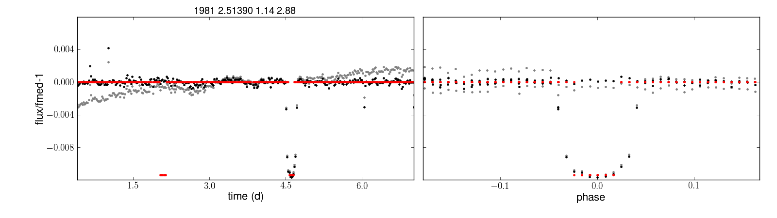
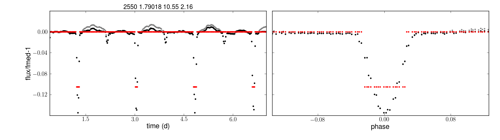
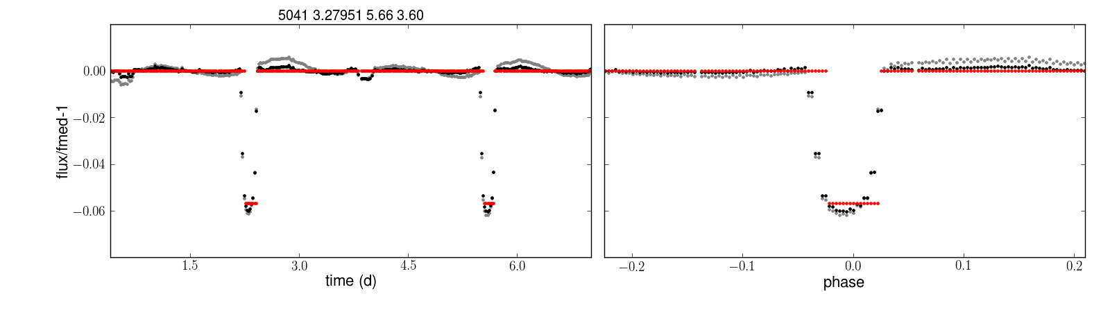
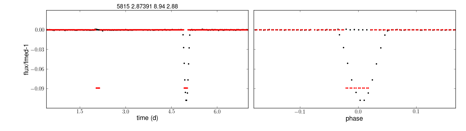
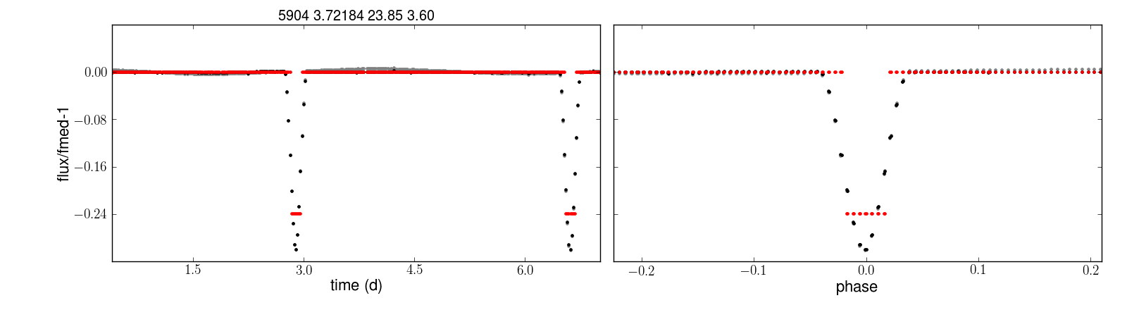
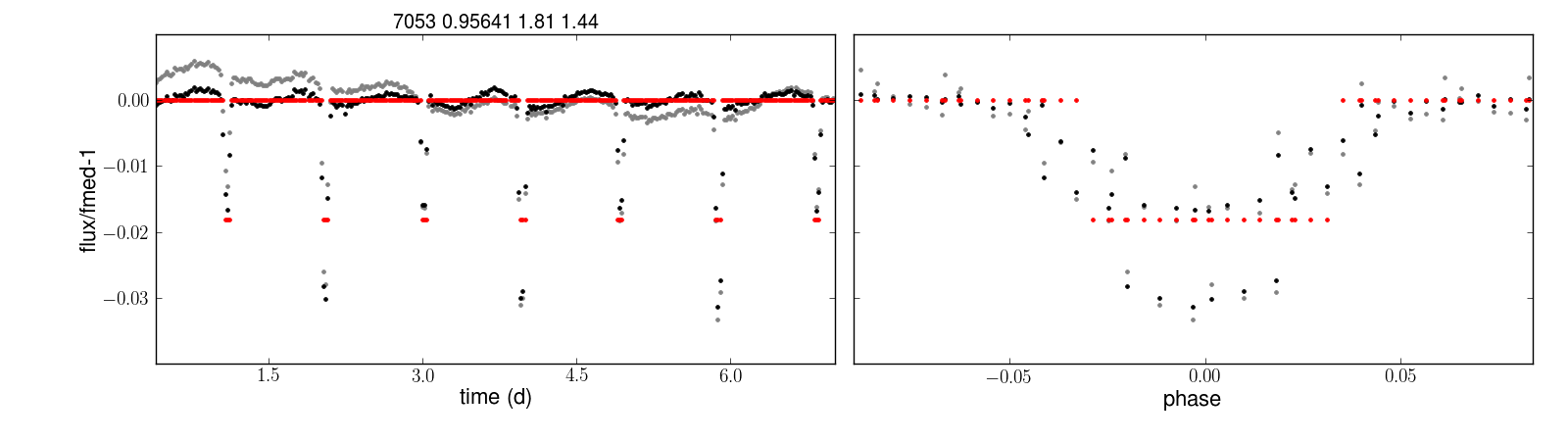
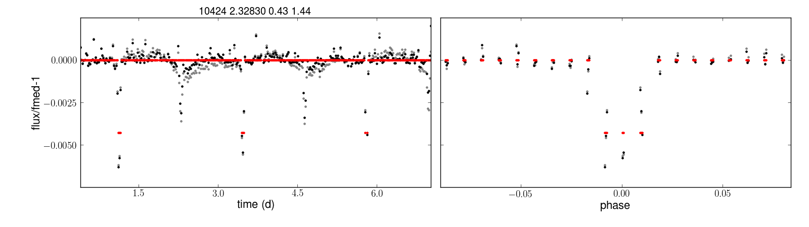
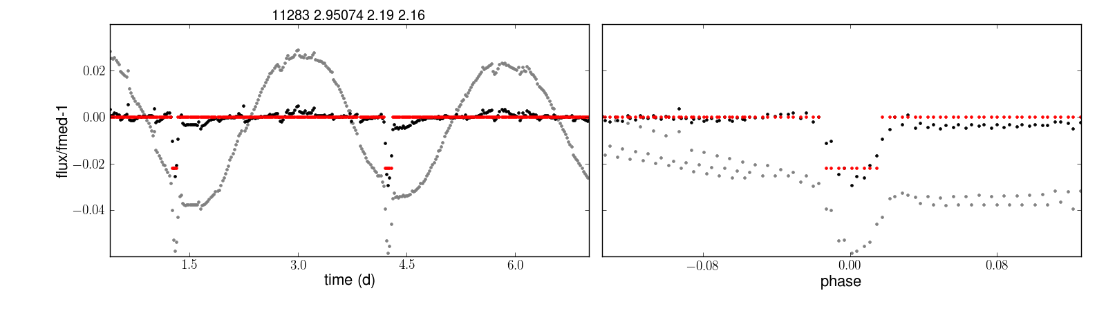
Figure 12: Transit candidates and detached eclipsing binaries identified in the transit search. Each pair of panels shows the unfolded and phase-folded light curves, respectively. In both panels, the original light curve is shown in grey, the light curve after removal of long-term trends in black, and the best-fit transit model in red.

Of these, two are bona-fide transit-like events: the known transiting planet WASP-28, and an astrophysical false positive (diluted eclipsing binary) previously identified by the XO project (Poleski et al., 2010). A further seven are clearly detached eclipsing binaries (EBs). Figure 12 illustrates the light curves for these nine objects. The adopted threshold also selected two objects which are clearly false positive – ‘detections’ caused by a single, low outlying data point. We experimented with outlier rejection schemes and found $5$-sigma clipping using a 3-point median filter effectively prevents this kind of false positives without affecting the rest of the detections. Finally, we detected 13 ‘classical’ variable stars – known RR Lyrae, $\delta$ Scuti and contact EBs, as well as a number of additional contact EBs for which we could not find evidence of a prior identification in the literature.

Overall, the results of the automated transit search are very encouraging: the number of candidates was manageable, clearly transit-like events were identified successfully, and the origin of the remainder of the detections was easy to identify.

6 Conclusions and future prospects

We have presented a new method to extract high-precision light curves from K2 data, combining list-driven aperture photometry with a semi-parametric correction of the systematic effects associated with the drift of the roll angle of the satellite about its boresight, which is performed on a star-by-star basis. Finally, we propose a simple prescription for selecting the aperture size depending on a target’s magnitude.

We achieve a photometric precision within a factor of 2–3 of the nominal Kepler mission performance. From the saturation limit ($K_{\rm p}\sim 9.5$) to $K_{\rm p}\sim 12$, most stars display scatters on transit timescales ranging from 30 to 100 ppm, while for fainter stars the precision is within a factor of 2 of the theoretical noise limit. Further improvements may be achieved in the near future by implementing a more sophisticated (spatially dependent) background correction, and more work is needed to understand the difference between our results and those of VJ14 for the brightest stars. One refinement we plan to test in the near future is to use non-circular apertures, given the significant elongation of the PSF at the edges of the Kepler FOV.

A strong point of our approach is that it preserves ‘real’ astrophysical variabitliy, which we demonstrated using both visual examination of individual examples and signal injection and recovery tests. Finally, we also performed a transit search on the objects brighter than $K{\rm p}=14$, successfully identifying the previously known transiting planet, transit-like EB and detached EBs in the sample.

6.1 Implications for planet detection

Our results and those of VJ14 have has very positive implications for the mission’s planet detection potential. They represent a factor $\sim 2$ or better improvement over H14’s early photometric precision estimates. This confirms the expectation that K2 should readily detect short-period gas and ice giants down to Neptune size around bright Sun-like stars, and planets down to Earth size around M-dwarfs. This is illustrated schematically in Figure 6, where the coloured arrows show the transit depth that such planets would cause compared to the detection limit in that light curve for 3 transits lasting 3 hours each.

6.2 Computational cost for full K2 campaigns

The photometric pipeline described in the present paper takes less than a day to run on a single Intel Xeon core, on the 9-day test dataset. To process full-length (85-day) K2 campaigns will require considerably more computing power: while the light curve extraction scales linearly with the amount of data, the GP regression involved in the systematics correction (which currently accounts for about half the total computing time) scales as the cubic power of the number of observation. It will thus go from about 1 to 100 seconds per star. This can be mitigated, however, by exploiting the almost perfectly regular time-sampling of the observations, and by using optimized matrix inversion schemes (as implemented for example in the george package, Ambikasaran et al. 2014), which can reduce the scaling from $N^{3}$ to $N^{2}$ or even $N\log N$. If we also consider the trivially parallelizable nature of most steps in our pipeline, we do not anticipate computational cost to be a major issue in applying the method presented here to future K2 datasets.

6.3 Extension to short-cadence

Our approach uses a global astrometric solution, which relies on the fact that there are enough stars observe across the FOV to obtain such a solution in a reliable way. This is true for long-cadence targets but will not, in general, hold for the much smaller number of short-cadence targets. Our method must therefore be modified qualitatively before it can be applied to short-cadence targets. This is a problem which we intend to address in the near future. In the meantime, a ‘shortcut’ might be to proceed as follows:

• use standard aperture photometry (fitting for the star’s position on each frame) to extract the raw light curve;

• interpolate the long-cadence roll-angle measurements to the sampling of short-cadence data;

• perform the systematics correction in the same way as for the long-cadence data, but fixing the amplitude and length scales of the time and roll-angle components of the GP model to the values obtained with long-cadence data, to keep the computational cost reasonable.

References

- Aigrain et al. (2007) Aigrain S., Hodgkin S., Irwin J., Hebb L., Irwin M., Favata F., Moraux E., Pont F., 2007, MNRAS, 375, 29
- Aigrain & Irwin (2004) Aigrain S., Irwin M., 2004, MNRAS, 350, 331
- Ambikasaran et al. (2014) Ambikasaran S., Foreman-Mackey D., Greengard L., Hogg D. W., O’Neil M., 2014, ArXiv e-prints
- Anderson et al. (2014) Anderson D. R., Collier Cameron A., Hellier C., Lendl M., Lister T. A., Maxted P. F. L., Queloz D., Smalley B., et al. 2014, A&A, submitted, arXiv:1402:1482
- Batalha et al. (2013) Batalha N. M., Rowe J. F., Bryson S. T., Barclay T., Burke C. J., Caldwell D. A., Christiansen J. L., Mullally F., Thompson S. E., et al. 2013, ApJS, 204, 24
- Borucki et al. (011a) Borucki W. J., Koch D. G., Basri G., Batalha N., Boss A., Brown T. M., Caldwell D., Christensen-Dalsgaard J., Cochran W. D., DeVore E., et al. 2011a, ApJ, 728, 117
- Borucki et al. (011b) Borucki W. J., Koch D. G., Basri G., Batalha N., Brown T. M., Bryson S. T., Caldwell D., Christensen-Dalsgaard J., Cochran W. D., DeVore E., et al. 2011b, ApJ, 736, 19
- Burke et al. (2014) Burke C. J., Bryson S. T., Mullally F., Rowe J. F., Christiansen J. L., Thompson S. E., Coughlin J. L., Haas M. R., Batalha N. M., et al. 2014, ApJS, 210, 19
- Byrd et al. (1995) Byrd R. H., Lu P., Nocedal A., 1995, SIAM Journal on Scientific and Statistical Computing, 16, 1190
- Christiansen et al. (2012) Christiansen J. L., Jenkins J. M., Caldwell D. A., Burke C. J., Tenenbaum P., Seader S., Thompson S. E., Barclay T. S., Clarke B. D., Li J., Smith J. C., Stumpe M. C., Twicken J. D., Van Cleve J., 2012, PASP, 124, 1279
- Gibson et al. (2012) Gibson N. P., Aigrain S., Roberts S., Evans T. M., Osborne M., Pont F., 2012, MNRAS, 419, 2683
- Howell et al. (2014) Howell S. B., Sobeck C., Haas M., Still M., Barclay T., Mullally F., Troeltzsch J., Aigrain S., Bryson S. T., Caldwell D., Chaplin W. J., Cochran W. D., Huber D., Marcy G. W., Miglio A., Najita J. R., Smith M., Twicken J. D., Fortney J. J., 2014, PASP, 126, 398
- Irwin et al. (2004) Irwin M. J., Lewis J., Hodgkin S., Bunclark P., Evans D., McMahon R., Emerson J. P., Stewart M., Beard S., 2004, in Quinn P. J., Bridger A., eds, Optimizing Scientific Return for Astronomy through Information Technologies Vol. 5493 of Society of Photo-Optical Instrumentation Engineers (SPIE) Conference Series, VISTA data flow system: pipeline processing for WFCAM and VISTA. pp 411–422
- Jenkins et al. (2010) Jenkins J. M., Caldwell D. A., Chandrasekaran H., Twicken J. D., Bryson S. T., Quintana E. V., Clarke B. D., Li J., Allen C., Tenenbaum P., Wu H., Klaus T. C., et al. 2010, ApJL, 713, L87
- Kovács et al. (2002) Kovács G., Zucker S., Mazeh T., 2002, A&A, 391, 369
- Nefs et al. (2012) Nefs S. V., Birkby J. L., Snellen I. A. G., Hodgkin S. T., Pinfield D. J., Sipőcz B., Kovacs G., Mislis D., et al. 2012, MNRAS, 425, 950
- Poleski et al. (2010) Poleski R., McCullough P. R., Valenti J. A., Burke C. J., Machalek P., Janes K., 2010, ApJS, 189, 134
- Rasmussen & Williams (2006) Rasmussen C. E., Williams C., 2006, Gaussian Processes for Machine Learning. The MIT Press
- Roberts et al. (2013) Roberts S., McQuillan A., Reece S., Aigrain S., 2013, MNRAS, 435, 3639
- Saito et al. (2012) Saito R. K., Hempel M., Minniti D., Lucas P. W., Rejkuba M., Toledo I., Gonzalez O. A., Alonso-García J., Irwin M. J., Gonzalez-Solares E., Hodgkin S. T., Lewis J. R., Cross N., et al. 2012, A&A, 537, A107
- Smith et al. (2012) Smith J. C., Stumpe M. C., Van Cleve J. E., Jenkins J. M., Barclay T. S., Fanelli M. N., Girouard F. R., Kolodziejczak J. J., McCauliff S. D., Morris R. L., Twicken J. D., 2012, PASP, 124, 1000
- Stellingwerf (1978) Stellingwerf R. F., 1978, ApJ, 224, 953
- Tamuz et al. (2005) Tamuz O., Mazeh T., Zucker S., 2005, MNRAS, 356, 1466
- Vanderburg & Johnson (2014) Vanderburg A., Johnson J. A., 2014, ApJ, in press, arXiv:1408:3853