From dependency to causality: a machine learning approach

Abstract

The relationship between statistical dependency and causality lies at the heart of all statistical approaches to causal inference. Recent results in the ChaLearn cause-effect pair challenge have shown that causal directionality can be inferred with good accuracy also in Markov indistinguishable configurations thanks to data driven approaches. This paper proposes a supervised machine learning approach to infer the existence of a directed causal link between two variables in multivariate settings with $n>2$ variables. The approach relies on the asymmetry of some conditional (in)dependence relations between the members of the Markov blankets of two variables causally connected. Our results show that supervised learning methods may be successfully used to extract causal information on the basis of asymmetric statistical descriptors also for $n>2$ variate distributions.

1 Introduction

The relationship between statistical dependency and causality lies at the heart of all statistical approaches to causal inference and can be summarized by two famous statements: correlation (or more generally statistical association) does not imply causation and causation induces a statistical dependency between causes and effects (or more generally descendants) ([26]). In other terms it is well known that statistical dependency is a necessary yet not sufficient condition for causality. The unidirectional link between these two notions has been used by many formal approaches to causality to justify the adoption of statistical methods for detecting or inferring causal links from observational data. The most influential one is the Causal Bayesian Network approach, detailed in ([17]) which relies on notions of independence and conditional independence to detect causal patterns in the data. Well known examples of related inference algorithms are the constraint-based methods like the PC algorithms ([30]) and IC ([23]). These approaches are founded on probability theory and have been shown to be accurate in reconstructing causal patterns in many applications. At the same time they restrict the set of configurations which causal inference is applicable to. Such boundary is essentially determined by the notion of distinguishability which defines the set of Markov equivalent configurations on the basis of conditional independence tests. Typical examples of indistinguishability are the two-variable setting and the completely connected triplet configuration ([12]) where it is impossible to distinguish between cause and effects by means of conditional or unconditional independence tests.

If on one hand the notion of indistinguishability is probabilistically sound, on the other hand it contributed to slow down the development of alternative methods to address interesting yet indistinguishable causal patterns. The slow down was in our opinion due to a misunderstanding of the meaning and the role of the notion of indistinguishability. Indistiguishability results rely on two main aspects: i) they refer only to specific features of dependency (notably conditional or unconditional independence) and ii) they state the conditions (e.g. faithfulness) under which it is possible to distinguish (or not) with certainty between configurations.

Accordingly, indistinguishability results do not prevent the existence of statistical algorithms able to reduce the uncertainty about the causal pattern even in indistinguishable configurations. This has been made evident by the appearance in recent years of a series of approaches which tackle the cause-effect pair inference, like ANM (Additive Noise Model) ([14]), IGCI (Information Geometry Causality Inference) ([9, 15]), LiNGAM (Linear Non Gaussian Acyclic Model) ([29]) and the algorithms described in ([21]) and ([31]). What is common to these approaches is that they use alternative statistical features of the data to detect causal patterns and reduce the uncertainty about their directionality. A further important step in this direction has been represented by the recent organization of the ChaLearn cause-effect pair challenge ([11]). The good (and significantly better than random) accuracy obtained on the basis of observations of pairs of causally related (or unrelated) variables supports the idea that alternative strategies can be designed to infer with success (or at least significantly better than random) indistinguishable configurations.

It is worthy to remark that the best ranked approaches in the ChaLearn competition share a common aspect: they infer from statistical features of the bivariate distribution the probability of the existence and then of the directionality of the causal link between two variables. The success of these approaches shows that the problem of causal inference can be successfully addressed as a supervised machine learning approach where the inputs are features describing the probabilistic dependency and the output is a class denoting the existence (or not) of a directed causal link. Once sufficient training data are made available, conventional feature selection algorithms ([13]) and classifiers can be used to return a prediction.

The effectiveness of machine learning strategies in the case of pairs of variables encourages the extension of the strategy to configurations with a larger number of variables. In this paper we propose an original approach to learn from multivariate observations the probability that a variable is a direct cause of another. This task is undeniably more difficult because

• the number of parameters needed to describe a multivariate distribution increases rapidly (e.g. quadratically in the Gaussian case),

• information about the existence of a causal link between two variables is returned also by the nature of the dependencies existing between the two variables and the remaining ones.

The second consideration is evident in the case of a collider configuration $\mathbf{z}_{1}\rightarrow\mathbf{z}_{2}\leftarrow\mathbf{z}_{3}$: in this case the dependency (or independency) between $\mathbf{z}_{1}$ and $\mathbf{z}_{3}$ tells us more about the link $\mathbf{z}_{1}\rightarrow\mathbf{z}_{2}$ than the dependency between $\mathbf{z}_{1}$ and $\mathbf{z}_{2}$. This led us to develop a machine learning strategy (described in Section 2) where descriptors of the relation existing between members of the Markov blankets of two variables are used to learn the probability (i.e. a score) that a causal link exists between two variables. The approach relies on the asymmetry of some conditional (in)dependence relations between the members of the Markov blankets of two variables causally connected. The resulting algorithm (called D2C and described in Section 3) predicts the existence of a direct causal link between two variables in a multivariate setting by (i) creating a set of of features of the relationship based on asymmetric descriptors of the multivariate dependency and (ii) using a classifier to learn a mapping between the features and the presence of a causal link.

In Section 4 we report the results of a set of experiments assessing the accuracy of the D2C algorithm. Experimental results based on synthetic and published data show that the D2C approach is competitive and often outperforms state-of-the-art methods.

2 Learning the relation between dependency and causality in a configuration with $n>2$ variables.

This section presents an approach to learn, from a number of observations, the relationships existing between the $n$ variate distribution of $\mathbf{Z}=[\mathbf{z}_{1},\dots,\mathbf{z}_{n}]$ and the existence of a directed causal link between two variables $\mathbf{z}_{i}$ and $\mathbf{z}_{j}$, $1\leq i\neq j\leq n$. Several parameters may be estimated from data in order to represent the multivariate distribution of $\mathbf{Z}$, like the correlation or the partial correlation matrix. Two problems however arise in this case: (i) these parameters are informative in case of Gaussian distributions only and (ii) identical (or close) causal configurations could be associated to very different parametric values, thus making difficult the learning of the mapping.

In other terms it is more relevant to describe the distribution in structural terms (e.g. with notions of conditional dependence/independence) rather than in parametric terms. Two more aspects have to be taken into consideration. First since we want to use a learning approach to identify cause-effect relationships we need some quantitative features to describe the structure of the multivariate distribution. Second, since asymmetry is a distinguishing characteristic of a causal relationship, we expect that effective features should share the same asymmetric properties.

In this paper we will use information theory to represent and quantify the notions of (conditional) dependence and independence between variables and to derive a set of asymmetric features to reconstruct causality from dependency.

2.1 Notions of information theory

Let us consider three continuous random variables $\mathbf{z}_{1}$, $\mathbf{z}_{2}$ and $\mathbf{z}_{3}$ having a joint Lebesgue density. Let us start by considering the relation between $\mathbf{z}_{1}$ and $\mathbf{z}_{2}$. The mutual information ([8]) between $\mathbf{z}_{1}$ and $\mathbf{z}_{2}$ is defined in terms of their probabilistic density functions $p(z_{1})$, $p(z_{2})$ and $p(z_{1},z_{2})$ as

$$I(\mathbf{z}_{1};\mathbf{z}_{2})=\int\int\log\frac{p(z_{1},z_{2})}{p(z_{1})p(z_{2})}p(z_{1},z_{2})dz_{1}dz_{2}=H(\mathbf{z}_{1})-H(\mathbf{z}_{1}|\mathbf{z}_{2})$$ (1)

where $H$ is the entropy and the convention $0\log\frac{0}{0}=0$ is adopted. This quantity measures the amount of stochastic dependence between $\mathbf{z}_{1}$ and $\mathbf{z}_{2}$ ([8]). Note that, if $\mathbf{z}_{1}$ and $\mathbf{z}_{2}$ are Gaussian distributed the following relation holds

$$I(\mathbf{z}_{1};\mathbf{z}_{2})=-\frac{1}{2}\log(1-\rho^{2})$$ (2)

where $\rho$ is the Pearson correlation coefficient between $\mathbf{z}_{1}$ and $\mathbf{z}_{2}$.

Let us now consider a third variable $\mathbf{z}_{3}$. The conditional mutual information ([8]) between $\mathbf{z}_{1}$ and $\mathbf{z}_{2}$ once $\mathbf{z}_{3}$ is given is defined by

$$I(\mathbf{z}_{1};\mathbf{z}_{2}|\mathbf{z}_{3})=\int\int\int\log\frac{p(z_{1},z_{2}|z_{3})}{p(z_{1}|z_{3})p(z_{2}|z_{3})}p(z_{1},z_{2},z_{3})dz_{1}dz_{2}dz_{3}=\\ =H(\mathbf{z}_{1}|\mathbf{z}_{3})-H(\mathbf{z}_{1}|\mathbf{z}_{2},\mathbf{z}_{3})$$ (3)

The conditional mutual information is null if and only if $\mathbf{z}_{1}$ and $\mathbf{z}_{2}$ are conditionally independent given $\mathbf{z}_{3}$.

A structural notion which can described in terms of conditional mutual information is the notion of Markov Blanket (MB). The Markov Blanket of variable $\mathbf{z}_{i}$ in an $n$ dimensional distribution is the smallest subset of variables belonging to $\mathbf{Z}\setminus\mathbf{z}_{i}$ (where $\setminus$ denotes the set difference operator) which makes $\mathbf{z}_{i}$ conditionally independent of all the remaining ones. In information theoretic terms let us consider a set $\mathbf{Z}$ of $n$ random variables, a variable $\mathbf{z}_{i}$ and a subset ${\mathbf{M}_{i}}\subset\mathbf{Z}\setminus\mathbf{z}_{i}$. The subset ${\mathbf{M}_{i}}$ is said to be a Markov blanket of $\mathbf{z}_{i}$ if it is the minimal subset satisfying

$$I(\mathbf{z}_{i};(\mathbf{Z}\setminus{(\mathbf{M}_{i}\cup\mathbf{z}_{i})})|{\mathbf{M}_{i}})=0$$

Effective algorithms have been proposed in literature to infer a Markov Blanket from observed data ([32]). Feature selection algorithms are also useful to construct a Markov blanket of a given target variable once they rely on notions of conditional independence to select relevant variables ([20]).

2.2 Causality and asymmetric dependency relationships

The notion of causality is central in science and also an intuitive notion of everyday life. The remarkable property of causality which distinguishes it from dependency is asymmetry.

In probabilistic terms a variable $\mathbf{z}_{i}$ is dependent on a variable $\mathbf{z}_{j}$ if the density of $\mathbf{z}_{i}$, conditional on the observation $\mathbf{z}_{j}=z_{j}$, is different from the marginal one

$$p(z_{i}|\mathbf{z}_{j}=z_{j})\neq p(z_{i})$$

In information theoretic terms the two variables are dependent if $I(\mathbf{z}_{i};\mathbf{z}_{j})=I(\mathbf{z}_{j};\mathbf{z}_{i})>0$. This implies that dependency is symmetric. If $\mathbf{z}_{i}$ is dependent on $\mathbf{z}_{j}$, then $\mathbf{z}_{j}$ is dependent on $\mathbf{z}_{i}$ too as shown by

$$p(z_{j}|\mathbf{z}_{i}=z_{i})\neq p(z_{j})$$

The formal representation of the notion of causality demands an extension of the syntax of the probability calculus as done by [22] with the introduction of the operator do which allows to distinguish the observation of a value of $\mathbf{z}_{j}$ (denoted by $\mathbf{z}_{j}=z_{j}$) from the manipulation of the variable $\mathbf{z}_{j}$ (denoted by $\tt{do}(\mathbf{z}_{j}=z_{j})$). Once this extension is accepted we say that a variable $\mathbf{z}_{j}$ is a cause of a variable $\mathbf{z}_{i}$ (e.g. ”diseases cause symptoms”) if the distribution of $\mathbf{z}_{i}$ is different from the marginal one when we set the value $\mathbf{z}_{j}=z_{j}$

$$p(z_{i}|{\tt do}(\mathbf{z}_{j}=z_{j}))\neq p(z_{i})$$

but not viceversa (e.g. ”symptoms do not cause disease”)

$$p(z_{j}|{\tt do}(\mathbf{z}_{i}=z_{i}))=p(z_{j})$$

The extension of the probability notation made by Pearl allows to formalize the intuition that causality is asymmetric. Another notation which allows to represent causal expression is provided by graphical models or more specifically by Directed Acyclic Graphs (DAG) ([17]). In this paper we will limit to consider causal relationships modeled by DAG, which proved to be convenient tools to understand and use the notion of causality. Furthermore we will make the assumption that the set of causal relationships existing between the variables of interest can be described by a Markov and faithful DAG ([23]). This means that the DAG is an accurate map of dependencies and independencies of the represented distribution and that using the notion of d-separation it is possible to read from the graph if two sets of nodes are (in)dependent conditioned on a third.

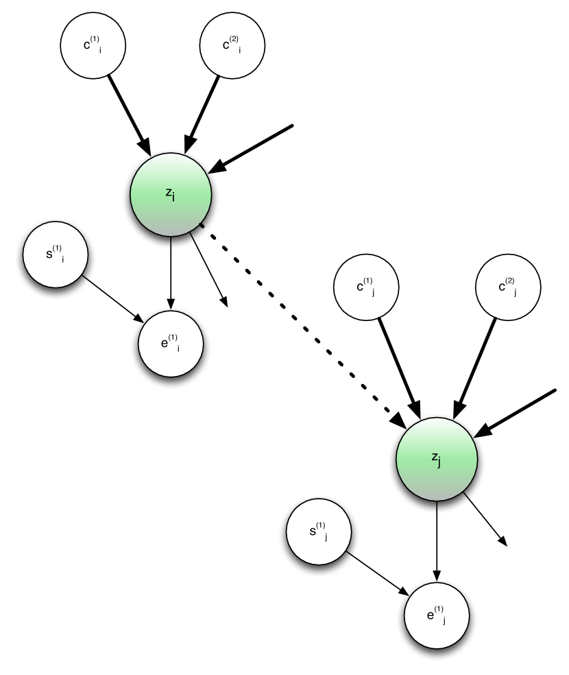
Figure 1: Two causally connected variables and their Markov Blankets.

The asymmetric nature of causality suggests that if we want to infer causal links from dependency we need to find some features (or descriptors) which describe the dependency and share with causality the property of asymmetry. Let us suppose that we are interested in predicting the existence of a directed causal link $\mathbf{z}_{i}\rightarrow\mathbf{z}_{j}$ where $\mathbf{z}_{i}$ and $\mathbf{z}_{j}$ are components of an observed $n$-dimensional vector $\mathbf{Z}=[\mathbf{z}_{1},\dots,\mathbf{z}_{n}]$.

We define as dependency descriptor of the ordered pair $\langle i,j\rangle$ a function $d(i,j)$ of the distribution of $\mathbf{Z}$ which depends on $i$ and $j$. Example of dependency descriptors are the correlation $\rho(i,j)$ between $\mathbf{z}_{i}$ and $\mathbf{z}_{j}$, the mutual information $I(\mathbf{z}_{i};\mathbf{z}_{j})$ or the partial correlation between $\mathbf{z}_{i}$ and $\mathbf{z}_{j}$ given another variable $\mathbf{z}_{k},i\neq j\neq k$.

We define a dependency descriptor symmetric if $d(i,j)=d(j,i)$ otherwise we call it asymmetric. Correlation or mutual information are symmetric descriptors since

$$d(i,j)=I(\mathbf{z}_{i};\mathbf{z}_{j})=I(\mathbf{z}_{j};\mathbf{z}_{i})=d(j,i)$$

Because of the asymmetric property of causality, if we want to maximize our chances to reconstruct causality from dependency we need to identify relevant asymmetric descriptors. In order to define useful asymmetric descriptors we have recourse to the Markov Blankets of the two variables $\mathbf{z}_{i}$ and $\mathbf{z}_{j}$.

Let us consider for instance the portion of a DAG represented in Figure 1 where the variable $\mathbf{z}_{i}$ is a direct cause of $\mathbf{z}_{j}$. The figure shows also the Markov Blankets of the two variables (denoted $M_{i}$ and $M_{j}$ respectively) and their components, i.e. the direct causes (denoted by $\mathbf{c}$), the direct effects ($\mathbf{e}$) and the spouses ($\mathbf{s}$) ([24]).

In what follows we will make two assumptions: (i) the only connection between the two sets is the edge $\mathbf{z}_{i}\rightarrow\mathbf{z}_{j}$ and (ii) there is no common ancestor of $\mathbf{z}_{i}$ ($\mathbf{z}_{j}$) and its spouses $\mathbf{s}_{i}$ ($\mathbf{s}_{j}$). We will discuss these assumptions at the end of the section. Given these assumptions and because of d-separation, a number of asymmetric conditional (in)dependence relations holds between the members of of $M_{i}$ and $M_{j}$ (Table 1). For instance (first line of Table 1), by conditioning on the effect $\mathbf{z}_{j}$ we create a dependence between $\mathbf{z}_{i}$ and the direct causes of $\mathbf{z}_{j}$ while by conditioning on the $\mathbf{z}_{i}$ we d-separate $\mathbf{z}_{j}$ and the direct causes of $\mathbf{z}_{i}$.

The relations in Table 1 can be used to define the following set of asymmetric descriptors,

$$d^{(k)}_{1}(i,j)=I(\mathbf{z}_{i};\mathbf{c}^{(k)}_{j}|\mathbf{z}_{j}),$$ (4)

$$d^{(k)}_{2}(i,j)=I(\mathbf{e}^{(k)}_{i};\mathbf{c}^{(k)}_{j}|\mathbf{z}_{j}),$$ (5)

$$d^{(k)}_{3}(i,j)=I(\mathbf{c}^{(k)}_{i};\mathbf{c}^{(k)}_{j}|\mathbf{z}_{j}),$$ (6)

$$d^{(k)}_{4}(i,j)=I(\mathbf{z}_{i};\mathbf{c}^{(k)}_{j}),$$ (7)

whose asymmetry is given by

$$d^{(k)}_{1}(i,j)=I(\mathbf{z}_{i};\mathbf{c}^{(k)}_{j}|\mathbf{z}_{j})>0,\quad d^{(k)}_{1}(j,i)=I(\mathbf{z}_{j};\mathbf{c}^{(k)}_{i}|\mathbf{z}_{i})=0,$$ (8)

$$d^{(k)}_{2}(i,j)=I(\mathbf{e}^{(k)}_{i};\mathbf{c}^{(k)}_{j}|\mathbf{z}_{j})>0,\quad d^{(k)}_{2}(j,i)=I(\mathbf{e}^{(k)}_{j};\mathbf{c}^{(k)}_{i}|\mathbf{z}_{i})=0,$$ (9)

$$d^{(k)}_{3}(i,j)=I(\mathbf{c}^{(k)}_{i};\mathbf{c}^{(k)}_{j}|\mathbf{z}_{j})>0,\quad d^{(k)}_{3}(j,i)=I(\mathbf{c}^{(k)}_{j};\mathbf{c}^{(k)}_{i}|\mathbf{z}_{i})=0,$$ (10)

$$d^{(k)}_{4}(i,j)=I(\mathbf{z}_{i};\mathbf{c}^{(k)}_{j})=0,\quad d^{(k)}_{4}(j,i)=I(\mathbf{z}_{j};\mathbf{c}^{(k)}_{i})>0.$$ (11)

Relation $i,j$	Relation $j,i$
$\forall k\quad\mathbf{z}_{i}\not\mathchoice{\mathrel{\hbox to0.0pt{$\displaystyle\perp$\hss}\mkern 2.0mu{\displaystyle\perp}}}{\mathrel{\hbox to0.0pt{$\textstyle\perp$\hss}\mkern 2.0mu{\textstyle\perp}}}{\mathrel{\hbox to0.0pt{$\scriptstyle\perp$\hss}\mkern 2.0mu{\scriptstyle\perp}}}{\mathrel{\hbox to0.0pt{$\scriptscriptstyle\perp$\hss}\mkern 2.0mu{\scriptscriptstyle\perp}}}\mathbf{c}^{(k)}_{j}|\mathbf{z}_{j}$	$\forall k\quad\mathbf{z}_{j}\mathchoice{\mathrel{\hbox to0.0pt{$\displaystyle\perp$\hss}\mkern 2.0mu{\displaystyle\perp}}}{\mathrel{\hbox to0.0pt{$\textstyle\perp$\hss}\mkern 2.0mu{\textstyle\perp}}}{\mathrel{\hbox to0.0pt{$\scriptstyle\perp$\hss}\mkern 2.0mu{\scriptstyle\perp}}}{\mathrel{\hbox to0.0pt{$\scriptscriptstyle\perp$\hss}\mkern 2.0mu{\scriptscriptstyle\perp}}}\mathbf{c}^{(k)}_{i}|\mathbf{z}_{i}$
$\forall k\quad\mathbf{e}^{(k)}_{i}\not\mathchoice{\mathrel{\hbox to0.0pt{$\displaystyle\perp$\hss}\mkern 2.0mu{\displaystyle\perp}}}{\mathrel{\hbox to0.0pt{$\textstyle\perp$\hss}\mkern 2.0mu{\textstyle\perp}}}{\mathrel{\hbox to0.0pt{$\scriptstyle\perp$\hss}\mkern 2.0mu{\scriptstyle\perp}}}{\mathrel{\hbox to0.0pt{$\scriptscriptstyle\perp$\hss}\mkern 2.0mu{\scriptscriptstyle\perp}}}\mathbf{c}^{(k)}_{j}|\mathbf{z}_{j}$	$\forall k\quad\mathbf{e}^{(k)}_{j}\mathchoice{\mathrel{\hbox to0.0pt{$\displaystyle\perp$\hss}\mkern 2.0mu{\displaystyle\perp}}}{\mathrel{\hbox to0.0pt{$\textstyle\perp$\hss}\mkern 2.0mu{\textstyle\perp}}}{\mathrel{\hbox to0.0pt{$\scriptstyle\perp$\hss}\mkern 2.0mu{\scriptstyle\perp}}}{\mathrel{\hbox to0.0pt{$\scriptscriptstyle\perp$\hss}\mkern 2.0mu{\scriptscriptstyle\perp}}}\mathbf{c}^{(k)}_{i}|\mathbf{z}_{i}$
$\forall k\quad\mathbf{c}^{(k)}_{i}\not\mathchoice{\mathrel{\hbox to0.0pt{$\displaystyle\perp$\hss}\mkern 2.0mu{\displaystyle\perp}}}{\mathrel{\hbox to0.0pt{$\textstyle\perp$\hss}\mkern 2.0mu{\textstyle\perp}}}{\mathrel{\hbox to0.0pt{$\scriptstyle\perp$\hss}\mkern 2.0mu{\scriptstyle\perp}}}{\mathrel{\hbox to0.0pt{$\scriptscriptstyle\perp$\hss}\mkern 2.0mu{\scriptscriptstyle\perp}}}\mathbf{c}^{(k)}_{j}|\mathbf{z}_{j}$	$\forall k\quad\mathbf{c}^{(k)}_{j}\mathchoice{\mathrel{\hbox to0.0pt{$\displaystyle\perp$\hss}\mkern 2.0mu{\displaystyle\perp}}}{\mathrel{\hbox to0.0pt{$\textstyle\perp$\hss}\mkern 2.0mu{\textstyle\perp}}}{\mathrel{\hbox to0.0pt{$\scriptstyle\perp$\hss}\mkern 2.0mu{\scriptstyle\perp}}}{\mathrel{\hbox to0.0pt{$\scriptscriptstyle\perp$\hss}\mkern 2.0mu{\scriptscriptstyle\perp}}}\mathbf{c}^{(k)}_{i}|\mathbf{z}_{i}$
$\forall k\quad\mathbf{z}_{i}\mathchoice{\mathrel{\hbox to0.0pt{$\displaystyle\perp$\hss}\mkern 2.0mu{\displaystyle\perp}}}{\mathrel{\hbox to0.0pt{$\textstyle\perp$\hss}\mkern 2.0mu{\textstyle\perp}}}{\mathrel{\hbox to0.0pt{$\scriptstyle\perp$\hss}\mkern 2.0mu{\scriptstyle\perp}}}{\mathrel{\hbox to0.0pt{$\scriptscriptstyle\perp$\hss}\mkern 2.0mu{\scriptscriptstyle\perp}}}\mathbf{c}^{(k)}_{j}$	$\forall k\quad\mathbf{z}_{j}\not\mathchoice{\mathrel{\hbox to0.0pt{$\displaystyle\perp$\hss}\mkern 2.0mu{\displaystyle\perp}}}{\mathrel{\hbox to0.0pt{$\textstyle\perp$\hss}\mkern 2.0mu{\textstyle\perp}}}{\mathrel{\hbox to0.0pt{$\scriptstyle\perp$\hss}\mkern 2.0mu{\scriptstyle\perp}}}{\mathrel{\hbox to0.0pt{$\scriptscriptstyle\perp$\hss}\mkern 2.0mu{\scriptscriptstyle\perp}}}\mathbf{c}^{(k)}_{i}$

Table 1: Asymmetric (un)conditional (in)dependance relationships between members of the Markov Blankets of $\mathbf{z}_{i}$ and $\mathbf{z}_{j}$ in Figure 1.

Relation $i,j$	Relation $j,i$
$\forall k\quad\mathbf{z}_{i}\not\mathchoice{\mathrel{\hbox to0.0pt{$\displaystyle\perp$\hss}\mkern 2.0mu{\displaystyle\perp}}}{\mathrel{\hbox to0.0pt{$\textstyle\perp$\hss}\mkern 2.0mu{\textstyle\perp}}}{\mathrel{\hbox to0.0pt{$\scriptstyle\perp$\hss}\mkern 2.0mu{\scriptstyle\perp}}}{\mathrel{\hbox to0.0pt{$\scriptscriptstyle\perp$\hss}\mkern 2.0mu{\scriptscriptstyle\perp}}}\mathbf{e}^{(k)}_{j}$	$\forall k\quad\mathbf{z}_{j}\not\mathchoice{\mathrel{\hbox to0.0pt{$\displaystyle\perp$\hss}\mkern 2.0mu{\displaystyle\perp}}}{\mathrel{\hbox to0.0pt{$\textstyle\perp$\hss}\mkern 2.0mu{\textstyle\perp}}}{\mathrel{\hbox to0.0pt{$\scriptstyle\perp$\hss}\mkern 2.0mu{\scriptstyle\perp}}}{\mathrel{\hbox to0.0pt{$\scriptscriptstyle\perp$\hss}\mkern 2.0mu{\scriptscriptstyle\perp}}}\mathbf{e}^{(k)}_{i}$
$\forall k\quad\mathbf{z}_{i}\mathchoice{\mathrel{\hbox to0.0pt{$\displaystyle\perp$\hss}\mkern 2.0mu{\displaystyle\perp}}}{\mathrel{\hbox to0.0pt{$\textstyle\perp$\hss}\mkern 2.0mu{\textstyle\perp}}}{\mathrel{\hbox to0.0pt{$\scriptstyle\perp$\hss}\mkern 2.0mu{\scriptstyle\perp}}}{\mathrel{\hbox to0.0pt{$\scriptscriptstyle\perp$\hss}\mkern 2.0mu{\scriptscriptstyle\perp}}}\mathbf{s}^{(k)}_{j}$	$\forall k\quad\mathbf{z}_{j}\mathchoice{\mathrel{\hbox to0.0pt{$\displaystyle\perp$\hss}\mkern 2.0mu{\displaystyle\perp}}}{\mathrel{\hbox to0.0pt{$\textstyle\perp$\hss}\mkern 2.0mu{\textstyle\perp}}}{\mathrel{\hbox to0.0pt{$\scriptstyle\perp$\hss}\mkern 2.0mu{\scriptstyle\perp}}}{\mathrel{\hbox to0.0pt{$\scriptscriptstyle\perp$\hss}\mkern 2.0mu{\scriptscriptstyle\perp}}}\mathbf{s}^{(k)}_{i}$
$\forall k\quad\mathbf{z}_{i}\mathchoice{\mathrel{\hbox to0.0pt{$\displaystyle\perp$\hss}\mkern 2.0mu{\displaystyle\perp}}}{\mathrel{\hbox to0.0pt{$\textstyle\perp$\hss}\mkern 2.0mu{\textstyle\perp}}}{\mathrel{\hbox to0.0pt{$\scriptstyle\perp$\hss}\mkern 2.0mu{\scriptstyle\perp}}}{\mathrel{\hbox to0.0pt{$\scriptscriptstyle\perp$\hss}\mkern 2.0mu{\scriptscriptstyle\perp}}}\mathbf{e}^{(k)}_{j}|\mathbf{z}_{j}$	$\forall k\quad\mathbf{z}_{j}\mathchoice{\mathrel{\hbox to0.0pt{$\displaystyle\perp$\hss}\mkern 2.0mu{\displaystyle\perp}}}{\mathrel{\hbox to0.0pt{$\textstyle\perp$\hss}\mkern 2.0mu{\textstyle\perp}}}{\mathrel{\hbox to0.0pt{$\scriptstyle\perp$\hss}\mkern 2.0mu{\scriptstyle\perp}}}{\mathrel{\hbox to0.0pt{$\scriptscriptstyle\perp$\hss}\mkern 2.0mu{\scriptscriptstyle\perp}}}\mathbf{e}^{(k)}_{i}|\mathbf{z}_{i}$
$\forall k\quad\mathbf{z}_{i}\mathchoice{\mathrel{\hbox to0.0pt{$\displaystyle\perp$\hss}\mkern 2.0mu{\displaystyle\perp}}}{\mathrel{\hbox to0.0pt{$\textstyle\perp$\hss}\mkern 2.0mu{\textstyle\perp}}}{\mathrel{\hbox to0.0pt{$\scriptstyle\perp$\hss}\mkern 2.0mu{\scriptstyle\perp}}}{\mathrel{\hbox to0.0pt{$\scriptscriptstyle\perp$\hss}\mkern 2.0mu{\scriptscriptstyle\perp}}}\mathbf{s}^{(k)}_{j}|\mathbf{z}_{j}$	$\forall k\quad\mathbf{z}_{j}\mathchoice{\mathrel{\hbox to0.0pt{$\displaystyle\perp$\hss}\mkern 2.0mu{\displaystyle\perp}}}{\mathrel{\hbox to0.0pt{$\textstyle\perp$\hss}\mkern 2.0mu{\textstyle\perp}}}{\mathrel{\hbox to0.0pt{$\scriptstyle\perp$\hss}\mkern 2.0mu{\scriptstyle\perp}}}{\mathrel{\hbox to0.0pt{$\scriptscriptstyle\perp$\hss}\mkern 2.0mu{\scriptscriptstyle\perp}}}\mathbf{s}^{(k)}_{i}|\mathbf{z}_{i}$
$\forall k\quad\mathbf{e}^{(k)}_{i}\mathchoice{\mathrel{\hbox to0.0pt{$\displaystyle\perp$\hss}\mkern 2.0mu{\displaystyle\perp}}}{\mathrel{\hbox to0.0pt{$\textstyle\perp$\hss}\mkern 2.0mu{\textstyle\perp}}}{\mathrel{\hbox to0.0pt{$\scriptstyle\perp$\hss}\mkern 2.0mu{\scriptstyle\perp}}}{\mathrel{\hbox to0.0pt{$\scriptscriptstyle\perp$\hss}\mkern 2.0mu{\scriptscriptstyle\perp}}}\mathbf{e}^{(k)}_{j}|\mathbf{z}_{i}$	$\forall k\quad\mathbf{e}^{(k)}_{j}\mathchoice{\mathrel{\hbox to0.0pt{$\displaystyle\perp$\hss}\mkern 2.0mu{\displaystyle\perp}}}{\mathrel{\hbox to0.0pt{$\textstyle\perp$\hss}\mkern 2.0mu{\textstyle\perp}}}{\mathrel{\hbox to0.0pt{$\scriptstyle\perp$\hss}\mkern 2.0mu{\scriptstyle\perp}}}{\mathrel{\hbox to0.0pt{$\scriptscriptstyle\perp$\hss}\mkern 2.0mu{\scriptscriptstyle\perp}}}\mathbf{e}^{(k)}_{i}|\mathbf{z}_{j}$
$\forall k\quad\mathbf{e}^{(k)}_{i}\mathchoice{\mathrel{\hbox to0.0pt{$\displaystyle\perp$\hss}\mkern 2.0mu{\displaystyle\perp}}}{\mathrel{\hbox to0.0pt{$\textstyle\perp$\hss}\mkern 2.0mu{\textstyle\perp}}}{\mathrel{\hbox to0.0pt{$\scriptstyle\perp$\hss}\mkern 2.0mu{\scriptstyle\perp}}}{\mathrel{\hbox to0.0pt{$\scriptscriptstyle\perp$\hss}\mkern 2.0mu{\scriptscriptstyle\perp}}}\mathbf{s}^{(k)}_{j}|\mathbf{z}_{j}$	$\forall k\quad\mathbf{e}^{(k)}_{j}\mathchoice{\mathrel{\hbox to0.0pt{$\displaystyle\perp$\hss}\mkern 2.0mu{\displaystyle\perp}}}{\mathrel{\hbox to0.0pt{$\textstyle\perp$\hss}\mkern 2.0mu{\textstyle\perp}}}{\mathrel{\hbox to0.0pt{$\scriptstyle\perp$\hss}\mkern 2.0mu{\scriptstyle\perp}}}{\mathrel{\hbox to0.0pt{$\scriptscriptstyle\perp$\hss}\mkern 2.0mu{\scriptscriptstyle\perp}}}\mathbf{s}^{(k)}_{i}|\mathbf{z}_{i}$

Table 2: Symmetric (un)conditional (in)dependance relationships between members of the Markov Blankets of $\mathbf{z}_{i}$ and $\mathbf{z}_{j}$ in Figure 1.

At the same time we can write a set of symmetric conditional (in)dependence relations (Table 2) and the equivalent formulations in terms of mutual information terms:

$$I(\mathbf{z}_{j};\mathbf{e}^{(k)}_{i})>0,$$ (12)

$$I(\mathbf{z}_{i};\mathbf{e}^{(k)}_{j})>0,$$ (13)

$$I(\mathbf{z}_{j};\mathbf{s}^{(k)}_{i})=I(\mathbf{z}_{i};\mathbf{s}^{(k)}_{j})=0,$$ (14)

$$I(\mathbf{z}_{i};\mathbf{e}_{j}^{(k)}|\mathbf{z}_{j})=I(\mathbf{z}_{j};\mathbf{e}_{i}^{(k)}|\mathbf{z}_{i})=I(\mathbf{z}_{i};\mathbf{s}_{j}^{(k)}|\mathbf{z}_{j})=I(\mathbf{z}_{j};\mathbf{s}_{i}^{(k)}|\mathbf{z}_{i})=0,$$ (15)

$$I(\mathbf{e}_{i}^{(k)};\mathbf{e}_{j}^{(k)}|\mathbf{z}_{j})=I(\mathbf{e}_{j}^{(k)};\mathbf{e}_{i}^{(k)}|\mathbf{z}_{i})=I(\mathbf{e}_{i}^{(k)};\mathbf{s}_{j}^{(k)}|\mathbf{z}_{j})=I(\mathbf{e}_{j}^{(k)};\mathbf{s}_{i}^{(k)}|\mathbf{z}_{i})=0.$$ (16)

2.3 From asymmetric relationships to distinct distributions

The asymmetric properties of the four descriptors (4)-(7) is encouraging if we want to exploit dependency related features to infer causal properties from data. However, this optimism is undermined by the fact that all the descriptors require already the capability of distinguishing between the causes (i.e. the terms $\mathbf{c}$) and the effects (i.e. the terms $\mathbf{e}$) of the Markov Blanket of a given variable. Unfortunately this discriminating capability is what we are looking for!

In order to escape this circularity problem we consider two solutions. The first is to have recourse to a preliminary phase that prioritizes the components of the Markov Blanket and then use this result as starting point to detect asymmetries and then improve the classification of causal links. This is for instance feasible by using a filter selection algorithm, like mIMR ([4]), which aims to prioritize the direct causes in the Markov Blanket by searching for pairs of variables with high relevance and low interaction.

The second solution is related to the fact that the asymmetry of the four descriptors induces a difference in the distributions of some information theoretic terms which do not require the distinction between causes and effects within the Markov Blanket. The consequence is that we can replace the descriptors (4)-(7) with other descriptors (denoted with the letter $D$) that can be actually estimated from data.

Let $\mathbf{m}^{(k)}$ denote a generic component of the Markov Blanket with no distinction between cause, effect or spouse. It follows that a population made of terms depending on $\mathbf{m}^{(k)}$ is a mixture of three subpopulations, the first made of causes, the second made of effects and the third of spouses, respectively. It follows that the distribution of the population is a finite mixture ([19]) of three distributions, the first related to the causes, the second to the effects and the third to the spouses. Since the moments of the finite mixture are functions of the moments of each component, we can derive some properties of the resulting mixture from the properties of each component. For instance if we can show that two subpopulations are identical but that all the elements of the third subpopulation in the first mixture are larger than the elements of the analogous subpopulation in the second mixture, we can derive that the two mixture distributions are different.

Consider for instance the quantity $I(\mathbf{z}_{i};\mathbf{m}^{(k_{j})}_{j}|\mathbf{z}_{j})$ where $\mathbf{m}^{(k_{j})}_{j}$, $k_{j}=1,\dots,K_{j}$ is a member of the set $M_{j}\setminus\mathbf{z}_{i}$. From (8) and (15) it follows that the mixture distribution associated to the populations ${D}_{1}(i,j)=\{I(\mathbf{z}_{i};\mathbf{m}_{j}^{(k_{j})}|\mathbf{z}_{j}),k_{j}=1,\dots,K_{j}\}$ and ${D}_{1}(j,i)=\{I(\mathbf{z}_{j};\mathbf{m}_{i}^{(k_{i})}|\mathbf{z}_{i}),k_{i}=1,\dots,K_{i}\}$ are different since

$$\begin{cases}I(\mathbf{z}_{i};\mathbf{m}_{j}^{(k_{j})}|\mathbf{z}_{j})>I(\mathbf{z}_{j};\mathbf{m}_{i}^{(k_{i})}|\mathbf{z}_{i}),\quad&\mbox{ if }\mathbf{m}_{j}^{(k_{j})}=\mathbf{c}_{j}^{(k_{j})}\land\mathbf{m}_{i}^{(k_{i})}=\mathbf{c}_{i}^{(k_{i})}\\ I(\mathbf{z}_{i};\mathbf{m}_{j}^{(k_{j})}|\mathbf{z}_{j})=I(\mathbf{z}_{j};\mathbf{m}_{i}^{(k_{i})}|\mathbf{z}_{i}),\quad&\mbox{else}\end{cases}$$ (17)

It follows that even if we are not able to distinguish between a cause $\mathbf{c}_{j}\in M_{j}$ and an effect $\mathbf{e}_{j}\in M_{j}$, we know that the distribution of the population ${D}_{1}(i,j)$ differs from the distribution of the population ${D}_{1}(j,i)$. We can therefore use the population ${D}_{1}(i,j)$ (or some of its moments) as descriptor of the causal dependency.

Similarly we can replace the descriptors (5), (6) with the distributions of the population ${D}_{2}(i,j)=\{I(\mathbf{m}_{i}^{(k_{i})};\mathbf{m}_{j}^{(k_{j})}|\mathbf{z}_{j}),k_{j}=1,\dots,K_{j},k_{i}=1,\dots,K_{i}\}$. From (9), (10) and (16) we obtain that the distributions of the populations ${D}_{2}(i,j)$ and ${D}_{2}(j,i)$ are different.

If we make the additional assumption that $I(\mathbf{z}_{j};\mathbf{e}^{(k)}_{i})=I(\mathbf{z}_{i};\mathbf{e}^{(k)}_{j})>0$ from (11) we obtain also that the distribution of the population ${D}_{3}(i,j)=\{I(\mathbf{z}_{i};\mathbf{m}_{j}^{(k_{j})}),k_{j}=1,\dots,K_{j}\}$ is different from the one of ${D}_{3}(j,i)=\{I(\mathbf{z}_{j};\mathbf{m}_{i}^{(k_{i})})$, $k_{i}=1,\dots,K_{i}\}$.

The previous results are encouraging and show that though we are not able to distinguish between the different components of a Markov Blanket, we can notwithstanding compute some quantities (in this case distributions of populations) whose asymmetry is informative about the causal relationships $\mathbf{z}_{i}\rightarrow\mathbf{z}_{j}$.

As a consequence by measuring from observed data some statistics (e.g. quantiles) related to the distribution of these asymmetric descriptors, we may obtain some insight about the causal relationship between two variables. This idea is made explicit in the algorithm described in the following section.

Though these results rely on the two assumptions made before, two considerations are worthy to be made. First, the main goal of the approach is to shed light on the existence of dependency asymmetries also in multivariate contributions. Secondly we expect that the second layer (based on supervised learning) will eventually compensate for configurations not compliant with the assumptions and take advantage of complementarity or synergy of the descriptors in discriminating between causal configurations.

3 The D2C algorithm

The rationale of the D2C algorithm is to predict the existence of a causal link between two variables in a multivariate setting by (i) creating a set of features of the relationship between the members of the Markov Blankets of the two variables and (ii) using a classifier to learn a mapping between the features and the presence of a causal link.

We use two sets of features to summarize the relation between the two Markov blankets: the first one accounts for the presence (or the position if the MB is obtained by ranking) of the terms of $M_{j}$ in $M_{i}$ and viceversa. For instance it is evident that if $\mathbf{z}_{i}$ is a cause of $\mathbf{z}_{j}$ we expect to find $\mathbf{z}_{i}$ highly ranked between the causal terms of $M_{j}$ but $\mathbf{z}_{j}$ absent (or ranked low) among the causes of $M_{i}$. The second set of features is based on the results of the previous section and is obtained by summarizing the distributions of the asymmetric descriptors with a set of quantiles.

We propose then an algorithm (D2C) which for each pair of measured variables $\mathbf{z}_{i}$ and $\mathbf{z}_{j}$:

1. infers from data the two Markov Blankets (e.g. by using state-of-the-art approaches) $M_{i}$ and $M_{j}$ and the subsets $M_{i}\setminus\mathbf{z}_{j}=\{\mathbf{m}^{(k_{i})},k_{i}=1,\dots,K_{i}\}$ and $M_{j}\setminus\mathbf{z}_{i}=\{\mathbf{m}^{(k_{j})},k_{j}=1,\dots,K_{j}\}$. Most of the existing algorithms associate to the Markov Blanket a ranking such that the most strongly relevant variables are ranked before.

2. computes a set of (conditional) mutual information terms describing the dependency between $\mathbf{z}_{i}$ and $\mathbf{z}_{j}$

   $$I=[I(\mathbf{z}_{i};\mathbf{z}_{j}),I(\mathbf{z}_{i};\mathbf{z}_{j}|\mbox{M}_{j}\setminus\mathbf{z}_{i}),I(\mathbf{z}_{i};\mathbf{z}_{j}|\mbox{M}_{i}\setminus\mathbf{z}_{j})]$$

3. computes the positions $P_{i}^{(k_{i})}$ of the members $\mathbf{m}^{(k_{i})}$ of $M_{i}\setminus\mathbf{z}_{j}$ in the ranking associated to $M_{j}\setminus\mathbf{z}_{i}$ and the positions $P_{j}^{(k_{j})}$ of the terms $\mathbf{m}^{(k_{j})}$ in the ranking associated to $M_{i}\setminus\mathbf{z}_{j}$. Note that in case of the absence of a term of $M_{i}$ in $M_{j}$, the position is set to $K_{j}+1$ (respectively $K_{i}+1$).

4. computes the populations based on the asymmetric descriptors introduced in Section 2.3:

   1. ${D}^{(1)}(i,j)=\{I(\mathbf{z}_{i};\mathbf{m}^{(k_{j})}_{j}|\mathbf{z}_{j}),k_{j}=1,\dots,K_{j}\}$

   2. ${D}^{(1)}(j,i)=\{I(\mathbf{z}_{j};\mathbf{m}^{(k_{i})}_{i}|\mathbf{z}_{i}),k_{i}=1,\dots,K_{i}\}$

   3. ${D}^{(2)}(i,j)=\{I(\mathbf{m}^{(k_{i})}_{i};\mathbf{m}^{(k_{j})}_{j}|\mathbf{z}_{i}),k_{i}=1,\dots,K_{i},k_{j}=1,\dots,K_{j}\}$ and

   4. ${D}^{(2)}(j,i)=\{I(\mathbf{m}^{(k_{i})}_{j};\mathbf{m}^{(k_{j})}_{i}|\mathbf{z}_{j}),k_{i}=1,\dots,K_{i},k_{j}=1,\dots,K_{j}\}$

   5. ${D}^{(3)}(i,j)=\{I(\mathbf{z}_{i};\mathbf{m}^{(k_{j})}_{j}),k_{j}=1,\dots,K_{j}\}$,

   6. ${D}^{(3)}(j,i)=\{I(\mathbf{z}_{j},\mathbf{m}^{(k_{i})}_{i}),k_{i}=1,\dots,K_{i}\}$

   where $k_{i}=1,\dots,K_{i}$, $k_{j}=1,\dots,K_{j}$

5. creates a vector of descriptors

   $$x=[I,\mathcal{Q}(\hat{P}_{i}),\mathcal{Q}(\hat{P}_{j}),\mathcal{Q}(\hat{D}^{(1)}(i,j)),\mathcal{Q}(\hat{D}^{(1)}(j,i)),\\ \mathcal{Q}(\hat{D}^{(2)}(i,j)),\mathcal{Q}(\hat{D}^{(2)}(j,i)),\mathcal{Q}(\hat{D}^{(3)}(i,j)),\mathcal{Q}(\hat{D}^{(3)}(j,i))]$$ (18)

   where $\hat{P}_{i}$ and $\hat{P}_{j}$ are the distributions of the populations $\{P_{i}^{(k_{i})}\}$ and $\{P_{j}^{(k_{j})}\}$ , $\hat{D}^{(h)}(i,j)$ denotes the distribution of the corresponding population $D^{(h)}(i,j)$ and $\mathcal{Q}$ returns a set of sample quantiles of a distribution (in the experiments we set the quantiles to 0.1, 0.25, 0.5, 0.75, 0.9).

The vector $x$ can be then derived from observational data and used to create a vector of descriptors to be used as inputs in a supervised learning paradigm.

The rationale of the algorithm is that the asymmetries between $M_{i}$ and $M_{j}$ (e.g. Table 1) induce an asymmetry on the distributions $\hat{P}$, and $\hat{D}$ and that the quantiles of those distributions provide information about the directionality of causal link ($\mathbf{z}_{i}\rightarrow\mathbf{z}_{j}$ or $\mathbf{z}_{j}\rightarrow\mathbf{z}_{i}$.) In other terms we expect that the distribution of these variables should return useful information about which is the cause and the effect. Note that these distributions would be more informative if we were able to rank the terms of the Markov Blankets by prioritizing the direct causes (i.e. the terms $\mathbf{c}_{i}$ and $\mathbf{c}_{j}$) since these terms play a major role in the asymmetries of Table 1. The D2C algorithm can then be improved by choosing an appropriate Markov Blanket selector algorithms, like the mIMR filter.

In the experiments (Section 4) we derive the information terms as difference between (conditional) entropy terms (see Equations (1) and (3)) which are themselves estimated by a Lazy Learning regression algorithm ([3]) by making an assumption of Gaussian noise. Lazy Learning returns a leave-one-out estimation of conditional variance which can be easily transformed in entropy under the normal assumption ([7]). The (conditional) mutual information terms are then obtained by using the relations (1) and (3).

3.1 Complexity analysis

As suggested by the reviewers it is interesting to make a complexity analysis of the approach: first it is important to remark that since the D2C approach relies on a classifier, its learning phase can be time-consuming and dependent on the number of samples and dimension. However, this step is supposed to be performed only once and from the user perspective it is more relevant to consider the cost in the testing phase. Given two nodes for which a test of the existence of a causal link is required, three steps have to be performed:

1. computation of the Markov blankets of the two nodes. The information filters we used have a complexity $O(Cn^{2})$ where $C$ is the cost of the computation of mutual information ([20]). In case of very large $n$ this complexity may be bounded by having the filter preceded by a ranking algorithm with complexity $O(Cn)$. Such ranking may limit the number of features taken into consideration by the filters to $n^{\prime}<n$ reducing then considerably the cost.

2. once a number $K_{i}$ ($K_{j}$) of members of MB_i (MB_j) have been chosen, the rest of the procedure has a complexity related to the estimation of a number $O(K_{i}K_{j})$ of descriptors. In this paper we used a local learning regression algorithm to estimate the conditional entropies terms. Given that each regression involves at most three terms, the complexity is essentially related linearly to the number $N$ of samples

3. the last step consists in the computation of the Random Forest predictions on the test set. Since the RF has been already trained, the complexity of this step depends only on the number of trees and not on the dimensionality or number of samples.

For each test, the resulting complexity has then a cost of the order $O(Cn+Cn^{\prime 2}+K_{i}K_{j}N)$. It is important to remark that an advantage of D2C is that, if we are interested in predicting the causal relation between two variables only, we are not forced to infer the entire adjacency matrix (as typically the case in constraint-based methods). This mean also that the computation of the entire matrix can be easily made parallel.

4 Experimental validation

In this section the D2C (Section 3) algorithm is assessed in a set of synthetic experiments and published datasets.

4.1 Synthetic data

This experimental session addresses the problem of inferring causal links from synthetic data generated for linear and non-linear DAG configurations of different sizes. All the variables are continuous, and the dependency between children and parents is modelled by the additive relationship

$$x_{i}=\sum\limits_{j\in par(i)}f_{i,j}(x_{j})+\epsilon_{i},\qquad i=1,\dots,n$$ (19)

where the noise $\epsilon_{i}\sim N(0,\sigma_{i})$ is Normal, $f_{i,j}(x)\in L(x)$ and three sets of continuous functions are considered:

• linear: $L(x)=\{f\mid f(x)=a_{0}+a_{1}x\}$

• quadratic: $L(x)=\{f\mid f(x)=a_{0}+a_{1}x+a_{2}x^{2}\}$

• sigmoid: $L(x)=\{f\mid f(x)=\frac{1}{exp(a_{0}+a_{1}x}\}$

In order to assess the accuracy with respect to dimensionality, we considered three network sizes:

• small: number of nodes $n$ is uniformly sampled in the interval $[20,30]$,

• medium: number of nodes $n$ is uniformly sampled in the interval $[100,200]$,

• large: number of nodes $n$ is uniformly sampled in the interval $[500,1000]$,
  

The assessment procedure relies on the generation of a number of DAG structures and the simulation, for each of them, of $N$ (uniformly random in $[100,500]$) node observations according to the dependency (19). In each dataset we removed the observations of five percent of the variables in order to introduce unobserved variables.

For each DAG, on the basis of its structure and the dataset of observations, we collect a number of pairs $\langle x_{d},y_{d}\rangle$, where $x_{d}$ is the descriptor vector returned by (18) and $y_{d}$ is the class denoting the existence (or not) of the causal link in the DAG topology.

The D2C training set is made of $D=6000$ pairs $\langle x_{d},y_{d}\rangle$ and is obtained by generating 750 DAGs and storing for each of them the descriptors associated to 4 positives examples (i.e. a pair where the node $z_{i}$ is a direct cause of $z_{j}$) and 4 negatives examples (i.e. a pair where the node $z_{i}$ is not a direct cause of $z_{j}$). A Random Forest classifier is trained on the balanced dataset: we use the implementation from the R package randomForest ([18]) with default setting.

The independent test set is obtained by considering an independent number of simulated DAGs. We consider 190 DAGs for the small and medium configurations and 90 for the large configuration. For each testing DAG we select 4 positives examples (i.e. a pair where the node $z_{i}$ is a direct cause of $z_{j}$) and 6 negatives examples (i.e. a pair where the node $z_{i}$ is not a direct cause of $z_{j}$). The predictive accuracy of the trained Random Forest classifier is then assessed on the test set.

The D2C approach is compared in terms of classification accuracy (Balanced Error Rate (BER)) to several state-of-the-art approaches implemented and described in the packages bnlearn ([28]), pcalg ([16]), and daglearn :

• DAGL1: DAG-Search score-based algorithm with potential parents selected with a L1 penalization ([27]).

• DAGSearch: unrestricted DAG-Search score-based algorithm (multiple restart greedy hill-climbing, using edge additions, deletions, and reversals) ([27]),

• DAGSearchSparse: DAG-Search score-based algorithm with potential parents restricted to the $10$ most correlated features ([27]),

• gs: Grow-Shrink constraint-based structure learning algorithm,

• hc: hill-climbing score-based structure learning algorithm,

• iamb: incremental association MB constraint-based structure learning algorithm,

• mmhc: max-min hill climbing hybrid structure learning algorithms,

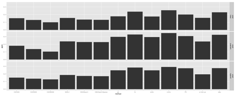
Figure 2: Balanced Error Rate of the different methods for small size DAGs and three types of dependency (top: linear, middle: quadratic, bottom: sigmoid). The notation D2Cx stands for D2C with a training set of size $x$.

• PC: Estimate the equivalence class of a DAG using the PC algorithm (this method was used only for the small size configuration (Figure 2) for computational time reasons)

• si.hiton.pc: Semi-Interleaved HITON-PC local discovery structure learning algorithms,

• tabu: tabu search score-based structure learning algorithm,

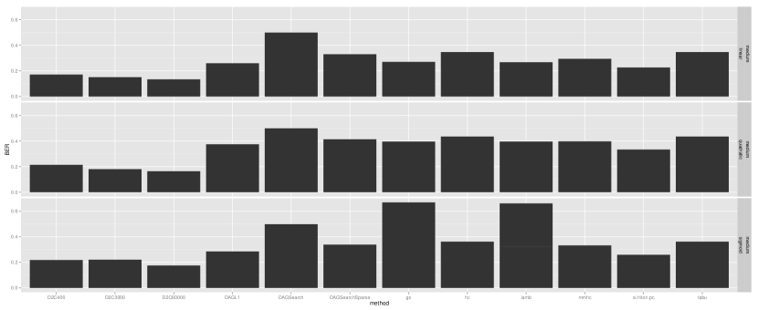
Figure 3: Balanced Error Rate of the different methods for medium size DAGs and three types of dependency (top: linear, middle: quadratic, bottom: sigmoid). The notation D2Cx stands for D2C with a training set of size $x$.

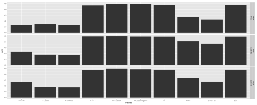
Figure 4: Balanced Error Rate of the different methods for large size DAGs and three types of dependency (top: linear, middle: quadratic, bottom: sigmoid). The notation D2Cx stands for D2C with a training set of size $x$.

The BER of three versions of the D2C method (training set size equal to 400, 3000 and 6000 respectively) are compared to the BER of state-of-the-art methods in Figures 2 (small), Figure 3 (medium) and Figure 4 (large). Each subfigure corresponds to the three types of stochastic dependency (top: linear, middle: quadratic, bottom: sigmoid).

A series of considerations can be made on the basis of the experimental results:

• the n-variate approach D2C obtains competitive results with respect to several state-of-the-art techniques in the linear case,

• the improvement of D2C wrt state-of-the-art techniques (often based on linear assumptions) tends to increase when we move to more nonlinear configurations,

• the accuracy of the D2C approach improves by increasing the number of training examples,

• with a small number of examples (i.e. $N=400$) it is already possible to learn a classifier D2C whose accuracy is competitive with state-of-the-art methods.

The D2C code is available in the CRAN R package D2C [5].

4.2 Published data

The second part of the assessment relies on the simulated and resimulated datasets proposed in ([1], Table 11). These 103 datasets were obtained by simulating data from known Bayesian networks and also by resimulation, where real data is used to elicit a causal network and then data is simulated from the obtained network. We split the 103 datasets in two portions: a training portion (made of 52 sets) and a second portion (made of 51 sets) for testing. This was done in order to assess the accuracy of two versions of the D2C algorithm: the first uses as training set only the samples generated in the previous section, the second includes in the training set also the 52 datasets of the training portion. The goal is to assess the generalization accuracy of the D2C algorithm with respect to DAG distributions never encountered before and not included in the training set. In this section we compare D2C to a set of algorithms implemented by the Causal Explorer software ([2]):

• GS: Grow/Shrink algorithm

• IAMB: Incremental Association-Based Markov Blanket

• IAMBnPC: IAMB with PC algorithm in the pruning phase

• interIAMBnPC: IAMB with PC algorithm in the interleaved pruning phase

and two filters based on information theory, mRMR ([25]) and mIMR ([4]). The comparison is done as follows: for each dataset and for each node (having at least a parent) the causal inference techniques return the ranking of the inferred parents. The ranking is assessed in terms of the average of Area Under the Precision Recall Curve (AUPRC) and a t-test is used to assess if the set of AUPRC values is significantly different between two methods. Note that the higher the AUPRC the more accurate is the inference method.

The summary of the paired comparisons is reported in Table 3 for the D2C algorithm trained on the synthetic data only and in Table 4 for the D2C algorithm trained on both synthetic data and the 52 training datasets.

	GS	IAMB	IAMBnPC	interIAMBnPC	mRMR	mIMR
W-L	48-3 (32-0)	43-8 (21-0)	46-5 (26-0)	46-5 (25-0)	42-9 (17-0)	34-17 (12-0)

Table 3: D2C trained on synthetic data only: number of datasets for which D2C has an AUPRC (significantly (pval $<0.05$)) higher/lower than the method in the column. W-L stands for Wins-Losses.

	GS	IAMB	IAMBnPC	interIAMBnPC	mRMR	mIMR
W-L	49-2 (36-0)	49-2 (27-0)	49-2 (32-0)	49-2 (32-0)	42-9 (17-0)	46-5 (19-1)

Table 4: D2C trained on synthetic data and 52 training datasets: number of datasets for which the D2C has an AUPRC (significantly (pval $<0.05$)) higher/lower than the method in the column. W-L stands for Wins-Losses.

It is worthy to remark that

• the D2C algorithm is extremely competitive and outperforms the other techniques taken into consideration,

• the D2C algorithm is able to generalize to DAG with different number of nodes and different distributions also when trained only on synthetic data simulated on linear DAGs,

• the D2C algorithm takes advantage from the availability of more training data and in particular of training data related to the causal inference task of interest, as shown by the improvement of the accuracy from Table 3 to Table 4,

• the two filters (mRMR and mIMR) algorithm appears to be the least inaccurate among the state-of-the-art algorithms,

• though the D2C is initialized with the results returned by the mIMR algorithm, it is able to improve its output and to significantly outperform it.

5 Conclusion

Two attitudes are common with respect to causal inference for observational data. The first is pessimistic and motivated by the consideration that correlation (or dependency) does not imply causation. The second is optimistic and driven by the fact that causation implies correlation (or dependency). This paper belongs evidently to the second school of thought and relies on the confidence that causality leaves footprints in the form of stochastic dependency and that these footprints can be detected to retrieve causality from observational data. The results of the ChaLearn challenge and the preliminary results of this paper confirm the potential of machine learning approaches in predicting the existence of causality links on the basis of statistical descriptors of the dependency. We are convinced that this will open a new research direction where learning techniques may be used to reduce the degree of uncertainty about the existence of a causal relationships also in indistinguishable configurations which are typically not addressed by conditional independence approaches.

Further work will focus on 1) discovering additional features of multivariate distributions to improve the accuracy 2) addressing and assessing other related classification problems (e.g. predicting if a variable is an ancestor or descendant of a given one) 3) extending the work to partial ancestral graphs (e.g. exploiting the logical relations presented in ([6])) 4 ) extending the validation to real datasets and configurations with a still larger number of variables (e.g. network inference in bioinformatics).

References

- [1] C. F. Aliferis, A. Statnikov, I. Tsamardinos, S. Mani, and X. D. Koutsoukos. Local causal and markov blanket induction for causal discovery and feature selection for classification. Journal of Machine Learning Research, 11:171–234, 2010.
- [2] C.F. Aliferis, I. Tsamardinos, and A. Statnikov. Causal explorer: A probabilistic network learning toolkit for biomedical discovery. In The 2003 International Conference on Mathematics and Engineering Techniques in Medicine and Biological Sciences (METMBS ’03), 2003.
- [3] G. Bontempi, M. Birattari, and H. Bersini. Lazy learning for modeling and control design. International Journal of Control, 72(7/8):643–658, 1999.
- [4] G. Bontempi and P.E. Meyer. Causal filter selection in microarray data. In Proceeding of the ICML2010 conference, 2010.
- [5] Gianluca Bontempi, Catharina Olsen, and Maxime Flauder. D2C: Predicting Causal Direction from Dependency Features, 2014. R package version 1.1.
- [6] Tom Claassen and Tom Heskes. A logical characterization of constraint-based causal discovery. In Proceedings of UAI 2011, 2011.
- [7] T. Cover and J.A. Thomas. Elements of Information Theory, 2nd ed. Wiley, 2006.
- [8] T. M. Cover and J. A. Thomas. Elements of Information Theory. John Wiley, New York, 1990.
- [9] P. Daniusis, D. Janzing, J. Mooij, J. Zscheischler, B. Steudel, K. Zhang, and B. Sch lkopf. Inferring deterministic causal relations. In Proceedings of the 26th Conference on Uncertainty in Artificial Intelligence (UAI-2010), pages 143–150, 2010.
- [10] C. Dethlefsen and S. Højsgaard. A common platform for graphical models in R: The gRbase package. Journal of Statistical Software, 14(17):1–12, 2005.
- [11] I. Guyon. Results and analysis of the 2013 ChaLearn cause-effect pair challenge. JMLR Workshop and Conference Proceedings, 2014.
- [12] I. Guyon, C. Aliferis, and A. Elisseeff. Computational Methods of Feature Selection, chapter Causal Feature Selection, pages 63–86. Chapman and Hall, 2007.
- [13] I. Guyon and A. Elisseeff. An introduction to variable and feature selection. Journal of Machine Learning Research, 3:1157–1182, 2003.
- [14] PO Hoyer, D. Janzing, J. Mooij, J. Peters, and B. Scholkopf. Nonlinear causal discovery with additive noise models. In Advances in Neural Information Processing Systems, pages 689–696, 2009.
- [15] D. Janzing, J. Mooij, K. Zhang, J. Lemeire, J. Zscheischler, P. Daniusis, B. Steudel, and B. Scholkopf. Information-geometric approach to inferring causal directions. Artificial Intelligence, 2012.
- [16] M. Kalisch, M. Mächler, D. Colombo, M. H. Maathuis, and P. Bühlmann. Causal inference using graphical models with the R package pcalg. Journal of Statistical Software, 47(11):1–26, 2012.
- [17] D. Koller and N. Friedman. Probabilistic graphical models. The MIT Press, 2009.
- [18] A. Liaw and M. Wiener. Classification and regression by randomforest. R News, 2(3):18–22, 2002.
- [19] G.J. McLaughlan. Finite Mixture Models. Wiley, 2000.
- [20] P.E. Meyer and G. Bontempi. Biological Knowledge Discovery Handbook, chapter Information-theoretic gene selection in expression data, page IEEE Computer Society. 2014.
- [21] JM Mooij, O. Stegle, D. Janzing, K. Zhang, and B. Sch lkopf. Probabilistic latent variable models for distinguishing between cause and effect. In Advances in Neural Information Processing Systems, 2010.
- [22] J. Pearl. Causal diagrams for empirical research. Biometrika, 82:669–710, 1995.
- [23] J. Pearl. Causality: models, reasoning, and inference. Cambridge University Press, 2000.
- [24] J.P. Pellet and A. Elisseeff. Using markov blankets for causal structure learning. Journal of Machine Learning Research, 9:1295–1342, 2008.
- [25] H. Peng, F. Long, and C. Ding. Feature selection based on mutual information: Criteria of max-dependency,max-relevance, and min-redundancy. IEEE Transactions on Pattern Analysis and Machine Intelligence, 27(8):1226–1238, 2005.
- [26] H. Reichenbach. The Direction of Time. University of California Press, Berkeley, 1956.
- [27] M. Schmidt, A. Niculescu-Mizil, and K. Murphy. Learning graphical model structure using l1-regularization paths. In Proceedings of the AAAI 2007 conference, 2007.
- [28] Marco Scutari. Learning bayesian networks with the bnlearn R package. Journal of Statistical Software, 35(3):1–22, 2010.
- [29] S. Shimizu, P.O. Hoyer, A. Hyv rinen, and A.J. Kerminen. A linear, non-gaussian acyclic model for causal discovery. Journal of Machine Learning Research, 7:2003–2030, 2006.
- [30] P. Spirtes, C. Glymour, and R. Scheines. Causation, Prediction and Search. Springer Verlag, Berlin, 2000.
- [31] A. Statnikov, M. Henaff, N.I. Lytkin, and C. F. Aliferis. New methods for separating causes from effects in genomics data. BMC Genomics, 13(S22), 2012.
- [32] I. Tsamardinos, C.F. Aliferis, and A. Statnikov. Algorithms for large scale markov blanket discovery. In Proceedings of the 16th International FLAIRS Conference (FLAIRS 2003), 2003.