Dynamics versus energetics in phase separation

Abstract

Phase separation may be driven by the minimization of a suitable free energy ${\cal F}$. This is the case, e.g., for diblock copolimer melts, where ${\cal F}$ is minimized by a steady periodic pattern whose wavelength $\lambda_{\hbox{\tiny GS}}$ depends on the segregation strength $\alpha^{-1}$ and it is know since long time that in one spatial dimension $\lambda_{\hbox{\tiny GS}}\simeq\alpha^{-1/3}$. Here we study in details the dynamics of the system in 1D for different initial conditions and by varying $\alpha$ by five orders of magnitude. We find that, depending on the initial state, the final configuration may have a wavelength $\lambda_{\hbox{\tiny D}}$ with $\lambda_{\hbox{\tiny min}}(\alpha)<\lambda_{\hbox{\tiny D}}<\lambda_{\hbox{\tiny max}}(\alpha)$, where $\lambda_{\hbox{\tiny min}}\approx\ln(1/\alpha)$ and $\lambda_{\hbox{\tiny max}}\approx\alpha^{-1/2}$. In particular, if the initial state is homogeneous, the system exhibits a logarithmic coarsening process which arrests whenever $\lambda_{\hbox{\tiny D}}\approx\lambda_{\hbox{\tiny min}}$.

Keywords: phase separation, pattern selection, coarsening

1 Introduction

A physical system quenched from a disordered, homogeneous phase into a coexistence region undergoes a phase ordering process [1] which is characterized by the minimization of the free energy ${\cal F}$. Very similar dynamics may appear in driven out of equilibrium systems [2], where the free energy is replaced by a suitable Lyapunov functional ${\cal F}_{\hbox{\tiny NE}}$. In both cases the final, equilibrium (or steady) state is expected to be the state which minimizes ${\cal F}$ (or ${\cal F}_{\hbox{\tiny NE}}$). Often, this minimal energy configuration is characterized by a finite wavelength or it corresponds to a complete phase separation, achieved via a coarsening process. As a matter of fact, the former picture (final fixed periodicity) can also be attained via a transient coarsening process.

It is worth to mention two limiting cases, the ordering of a binary alloy and the Rayleigh-Bénard pattern formation close to the convective threshold. The former problem can be described by the Cahn-Hilliard (CH) equation [3], which is known to be characterized by a perpetual coarsening process. The second phenomenon is usually described by the Swift-Hohenberg (SH) equation [2], whose behavior close to the instability threshold is universal for stationary type-I instabilities [2]: it is characterized by the emergence of a periodic pattern whose modulation undergoes a secondary instability, the so-called Eckhaus instability [4], a transient process during which rolls are locally created or destroyed until a stable roll size is attained.

Both CH and SH equations are characterized by an homogeneous phase which is linearly unstable in a range $(q_{1},q_{2})$ of wavevectors, with the difference that $q_{1}=0$ for CH and $q_{1}\simeq q_{2}\simeq q_{c}$ for SH. However, there is an even more important difference between the two. All CH periodic steady states are unstable, while SH periodic steady states are stable in a finite $q-$interval around the value which minimizes the SH free energy. The existence of such stable interval cannot ensure the ground state is dynamically attained. In the absence of noise it is almost certainly not attained and even if noise is present, the time scale might be too large to be experimentally observed. However, in the SH problem near the threshold, the final state is always very close to the ground state, because the interval $(q_{1},q_{2})$ is a small interval around a finite value $q_{\hbox{\tiny c}}$.

A physical problem which has long been studied [5, 6, 7, 8, 9, 10, 11, 12] and which is related to both limiting cases discussed here above (CH and SH) is the phase separation in diblock copolymer melts. In this example two different subchains $A$ and $B$ compose a chain molecule. In the disordered phase $A$ and $B$ are well mixed, but below $T_{\hbox{\tiny c}}$ there is a tendency to segregation which is never complete, because of a long range term in the free energy which stabilizes the system at a certain length scale depending on the strength of segregation, $\alpha^{-1}$ (see next Section). For infinite segregation strength $(\alpha=0)$ the system behaves as a binary alloy and it is described by the CH equation. For weak segregation there is a rapid selection of the size of the pattern, described by the SH equation.

In the seminal paper by Liu and Goldenfeld [6], authors focus on $\lambda_{\hbox{\tiny GS}}$, the wavelength of the pattern which minimizes the free energy. They find numerically $\lambda_{\hbox{\tiny GS}}\approx\alpha^{-1/4}$ for $\alpha>10^{-2}$ and $\lambda_{\hbox{\tiny GS}}\approx\alpha^{-1/3}$ for vanishing $\alpha$. We are interested to the second regime and all our results refer to the limit of very small $\alpha$. The other regime has been recently addressed by Benilov et al. [11], who study in detail how the region of stable patterns widens with decreasing $\alpha$, starting from the SH limit.

Comprehensive studies on the dynamics of this system with varying $\alpha$ and with varying initial conditions are absent. Therefore, in this manuscript we focus on dynamics in the regime of small $\alpha$, showing the existence of a range $(q_{\hbox{\tiny s1}},q_{\hbox{\tiny s2}})=(2\pi/\lambda_{\hbox{\tiny max}},2\pi/\lambda_{\hbox{\tiny min}})$ of wavevectors where steady states are stable and whose extrema both vanish with $\alpha$, according to well defined laws: $q_{\hbox{\tiny s1}}\approx\sqrt{\alpha}$ and $q_{\hbox{\tiny s2}}\approx-1/\ln\alpha$. If phase ordering starts from the disordered state, the final configuration is essentially determined by $q_{\hbox{\tiny s2}}=2\pi/\lambda_{\hbox{\tiny min}}$, which is attained via a logarithmic coarsening process.

In Sec. 2 we define the model, set the relevant notations and questions, and discuss the energetics. In Sec. 3 we report our results on dynamics, which are discussed in the final Sec. 4.

2 The model and the energetics

The model equation we are using to study the problem of phase separation is the so-called Oono-Shiwa [5] (OS) equation,

$$\frac{\partial u}{\partial t}=-\partial_{xx}\left(u_{xx}+u-u^{3}\right)-\alpha u$$ (1)

which depends on one parameter only, $\alpha$, because the coefficients of the other terms can be set to one by a suitable rescaling of $u,x,$ and $t$.

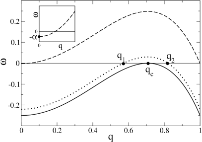
Figure 1: The linear stability spectrum for $\alpha=0.002,0.22,0.25$ (from top to bottom). The explicit values of $q_{1,2}(\alpha)$ are given in Eq. (3). The case $\alpha=0.002$ (dashed line) is enlarged in the inset around $q=0$, to stress that $\omega(q\to 0)<0$ for any $\alpha>0$.

The linear stability analysis of the homogeneous phase $u\equiv 0$ is easily obtained assuming $u(x,t)=u_{0}\exp(\omega t+iqx)$ and linearizing Eq. (1) in $u_{0}$. We get

$$\omega(q)=-\alpha+q^{2}-q^{4},$$ (2)

which is plotted in Fig. 1. Therefore, the equation is linearly unstable $(\omega(q)>0$) for $q_{1}<|q|<q_{2}$, where

$$q_{1}=\left(\frac{1}{2}-\sqrt{\frac{1}{4}-\alpha}\,\right)^{1/2}\quad\mbox{and}\quad q_{2}=\left(\frac{1}{2}+\sqrt{\frac{1}{4}-\alpha}\,\right)^{1/2}$$ (3)

and the most unstable mode is $q_{\hbox{\tiny c}}=\frac{1}{\sqrt{2}}$, with $\omega(q_{\hbox{\tiny c}})=\frac{1}{4}-\alpha$.

The Oono-Shiwa equation trivially reduces to the Cahn-Hilliard equation for $\alpha=0$. It is well known [13] that in this limit we get perpetual logarithmic coarsening and the asymptotic profile is a sequence of kinks (and antikinks) [14], which represent finite size domain walls interpolating between the stable solutions $u=-1$ and $u=+1$ (or viceversa). However, the OS equation has another interesting limit: for $\alpha\to(\frac{1}{4})^{-}$, it displays the well known Eckhaus instability. We expect this limit from Eq. (2) and from the nature of the nonlinear term, which is a cubic term. In fact, in the limit $\alpha\to(\frac{1}{4})^{-}$ the range of stable states has been determined in [11] and it coincides with the Eckhaus scenario, which is reproduced, for the sake of completeness, in A.

More precisely, the existence of this limit means that, if $\alpha=\frac{1}{4}-\epsilon^{2}$ with $\epsilon\ll 1$, the linearly unstable interval of the homogeneous phase is $(q_{1},q_{2})=(q_{c}-\delta,q_{c}+\delta)$, with $\delta=\epsilon/\sqrt{2}$. For any $q$ belonging to such interval there is a steady state, but only those belonging to the narrower subinterval $(q_{c}-\delta/\sqrt{3},q_{c}+\delta/\sqrt{3})$ are stable.

Let us now introduce the free energy whose minimization drives the dynamics. The OS equation can be written in a variational form [5],

$$\partial_{t}u(x,t)=\partial_{xx}\frac{\delta{\cal F}_{\hbox{\tiny OS}}}{\delta u}$$ (4)

where

$${\cal F}_{\hbox{\tiny OS}}[u]=\int dx\left[\frac{1}{2}u_{x}^{2}+\left(-\frac{u^{2}}{2}+\frac{u^{4}}{4}\right)\right]-\frac{\alpha}{4}\int dx\int dx^{\prime}u(x,t)|x-x^{\prime}|u(x^{\prime},t).\qquad$$ (5)

If we define the density of free energy, $\tilde{\cal F}_{\hbox{\tiny OS}}[u]=L^{-1}{\cal F}_{\hbox{\tiny OS}}[u]$ with $L$ meaning the total extension of the system in the $x-$direction, for a periodic configuration of wavelength $\lambda$ we get

$$\tilde{\cal F}_{\hbox{\tiny OS}}[u]=\left\langle\left[\frac{1}{2}u_{x}^{2}+\left(-\frac{u^{2}}{2}+\frac{u^{4}}{4}\right)\right]\right\rangle-\frac{\alpha}{4\lambda}\int_{-\lambda/2}^{\lambda/2}dx\int_{-\lambda/2}^{\lambda/2}dx^{\prime}u(x)|x-x^{\prime}|u(x^{\prime}).\qquad$$ (6)

The former expression cannot be evaluated analytically in an exact manner, because steady states of OS Eq. (1) are not known. However, it has been evaluated either numerically [6] or analytically in an approximate way [10], giving consistent results: for small $\alpha$, $\tilde{\cal F}_{\hbox{\tiny OS}}[u]$ is minimised for $\lambda=\lambda_{\hbox{\tiny GS}}\approx\alpha^{-1/3}$. Because of its simplicity we give here a brief derivation of this result.

The underlying idea, suggested by numerical sumulations and by dimensional analysis of Eq. (1), is the following: if we start from the homogeneous solution, represented by white noise $u(x,t)=\eta(x,t)$, the term $\alpha u$ which distinguish OS from CH equation comes into play for $t\approx\alpha^{-1}$: at short times the dynamics is the coarsening process as given by the CH equation, but this process stops when $t\approx\alpha^{-1}$. If this picture is correct, it is reasonable to evaluate Eq. (6) using the steady states for $\alpha=0$.

The average value $\langle[\dots]\rangle$ on the RHS of Eq. (6) has the form $\langle\frac{1}{2}u_{x}^{2}+V(u)\rangle$, with $V(u)=-(u^{2}/2)+(u^{4}/4)$, and steady states satisfy the equation  $\frac{1}{2}u_{x}^{2}-V(u)=\frac{1}{4}$, so that

$$\left\langle\frac{1}{2}u_{x}^{2}+V(u)\right\rangle=\langle u_{x}^{2}\rangle-\frac{1}{4}.$$ (7)

The function $u_{x}^{2}$ is concentrated at kink positions. If $\tilde{u}(x)=\tanh(x/\sqrt{2})$ is the kink profile centred in $x=0$, we can write

$$\langle u_{x}^{2}\rangle\simeq\frac{4}{\lambda}\int_{0}^{\lambda/4}dx\frac{1}{2\cosh^{4}(x/\sqrt{2})}\simeq\frac{8\sqrt{2}}{\lambda}\left(1-e^{-\lambda/\sqrt{2}}\right).$$ (8)

The leading term, $\langle u_{x}^{2}\rangle\simeq\frac{8\sqrt{2}}{\lambda}$, is sufficient here.

The term proportional to $\alpha$ in Eq. (6) can be evaluated in the simplest way by approximating the kink profile by a step function, $\tilde{u}(x)=\pm 1$ for $x\gtrless 0$, getting (see Eq. (6))

$$-\frac{\alpha}{4\lambda}\int_{-\lambda/2}^{\lambda/2}dx\int_{-\lambda/2}^{\lambda/2}dx^{\prime}u(x)|x-x^{\prime}|u(x^{\prime})\approx\frac{\alpha}{24}\lambda^{2}.$$ (9)

Summing up terms in Eq. (6) we have

$$\tilde{\cal F}_{\hbox{\tiny OS}}[u]=\frac{8\sqrt{2}}{\lambda}+\frac{\alpha}{24}\lambda^{2}-\frac{1}{4},$$ (10)

which has a minimum for

$$\lambda_{\hbox{\tiny GS}}=\left(\frac{96\sqrt{2}}{\alpha}\right)^{1/3}\approx\frac{5}{\alpha^{1/3}}.$$ (11)

Above result, which can be refined within the same spirit [10], is in agreement with the original numerical analysis by Liu and Goldenfeld [6], which also gives $\lambda_{\hbox{\tiny GS}}\approx\alpha^{-1/3}$ for small $\alpha$.

3 Dynamics

In the previous Section we have shown that, according to energetics, the final wavelength should scale with the segregation strength as $\alpha^{-1/3}$. Here we are going to study dynamics instead. For this purpose, we have solved numerically the OS equation (1) for $5\times 10^{-7}<\alpha<8\times 10^{-2}$, using a time splitting pseudo spectral code, whose details are given in C.1.

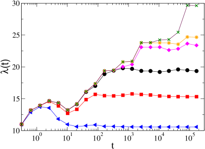
Figure 2: (Color online) (a) Spatial profiles of $u(x,t)$ for $\alpha=10^{-2}$ and $t=0.32,20.5,16777$ (from bottom to top). (b) The time dependence of the typical wavelength $\lambda(t)$ for $\alpha=10^{-1},10^{-2},10^{-3},10^{-4},10^{-5},10^{-6}$ (from bottom to top). The data refer to random initial conditions, $L=\sqrt{2}\pi\times 100$, time step $\Delta t=0.0025$ and 1024 Fourier modes (corresponding to a spatial resolution $\Delta x=0.43$).

In Fig. 2(a) we plot the profile for $\alpha=10^{-2}$ at short time (bottom), intermediate time (center), and after saturation of the wavelength (top). Initial conditions correspond to a random profile (more details are given in C.2). In plate (b) of the same figure we show the typical wavelength of the structure, $\lambda(t)$, as a function of time, when varying $\alpha$ (which decreases from bottom to top). These results give a qualitative proof of a few relevant features of our system, already discussed in Sec. 2: (i) the system coarsens for a finite time; (ii) the coarsening dynamics does not depend on $\alpha$; (iii) the final wavelength increases with decreasing $\alpha$. The non monotonous behavior of $\lambda(t)$ is a well known feature which goes beyond the OS model (see, e.g., Figs. 7,8 of [15] and Fig. 6 of [16]). It has the same interpretation as the non monotonous behavior of the roughness [17].

Figure 3: (a) Steady spatial profiles $u(x,t\to\infty)$ for $\alpha=10^{-1},10^{-2},10^{-3}$ (from bottom to top). Shown configurations refer to a time $t=16777$, $L=\sqrt{2}\pi\times 100$, time step $\Delta t=0.0025$ and 1024 Fourier modes. (b) The asymptotic length of the structure, $\langle\lambda_{\hbox{\tiny D}}(\alpha)\rangle=\langle\lambda(t\to\infty,\alpha)\rangle$, has been obtained by integrating the system up to time $\simeq 10^{5}$, starting from a random initial configuration, and by averaging over $10-30$ different initial conditions (noise realizations). The data refer to $L=\sqrt{2}\pi\times 40$, time step $\Delta t=0.0025$ and 1024 Fourier modes, corresponding to $\Delta x=0.17$. The straight line is a best fitting and corresponds to the function $\lambda_{\hbox{\tiny D}}=4.37-1.88\ln\alpha$.

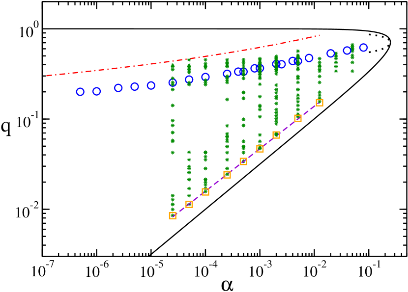
Figure 4: (Color online) The stability diagram $(q,\alpha)$: the (green) asterisks and the (blue) circles indicate stable solutions found via direct numerical simulations. Circles have been obtained by starting from random initial conditions and they are the same data plotted in lin-log scale in Fig. 3b. The initial conditions for asterisks are of various types, discussed in the main text and in C.2. (Orange) squares are the minimal stable $q^{\prime}$s for any $\alpha\leq 0.01$. We also plot the power law fitting $\simeq 1.22\times\alpha^{0.47}$ (dashed violet line). The (red) dot-dashed line denotes the theoretical estimate, Eq. (14), of the upper bound for the stability of the wave vectors. For the details on the performed simulations see C. Black, dotted lines are the analytical curves $q_{\hbox{\tiny s1,s2}}(\alpha)$ in the Eckhaus limit $\alpha\to 1/4$.

Now, let us focus on the final configurations, see Fig. 3. In (a) we give the profiles at different $\alpha$ and in (b) we plot $\lambda_{\hbox{\tiny D}}(\alpha)=\lambda(t\to\infty,\alpha)$, which increases logarithmically as $\lambda_{\hbox{\tiny D}}\approx\ln(1/\alpha)$. These results are not surprising, even if the actual evaluation of $\lambda_{\hbox{\tiny D}}(\alpha)$ should be new at our knowledge. Let us now discuss the main results of our paper, which are contained in Fig. 4 where we plot the stability diagram of the Oono-Shiwa equation in the plane $(\alpha,q)$. The thick line has two branches, corresponding to $q_{\hbox{\tiny 1,2}}(\alpha)$, the extrema of the interval where the homogeneous solution $u=0$ is linearly unstable. When $\alpha\to\frac{1}{4}$, $q_{\hbox{\tiny 1,2}}(\alpha)\to q_{\hbox{\tiny c}}=1/\sqrt{2}$ and the Eckhaus scenario applies [2]. This means that a steady state exists for any $q\in(q_{1},q_{2})=(q_{\hbox{\tiny c}}-\delta,q_{\hbox{\tiny c}}+\delta)$, where $\delta=(1/4-\alpha)^{2}$. If $q\in(q_{\hbox{\tiny s1}},q_{\hbox{\tiny s2}})=(q_{\hbox{\tiny c}}-\frac{\delta}{\sqrt{3}},q_{\hbox{\tiny c}}+\frac{\delta}{\sqrt{3}})$, the steady state is stable, otherwise it is unstable and dynamics proceeds until the final wavevector is in the stable range. In Fig. 4 we plot as dotted lines the analytical curves $q_{\hbox{\tiny s1,s2}}(\alpha)$ in the Eckhaus limit. The range $10^{-2}<\alpha<\frac{1}{4}$ has been studied in [11], we are interested to the regime of small $\alpha$.

Two main questions should be faced. Firstly, how do the extrema of the stable region, $(q_{\hbox{\tiny s1}}(\alpha),q_{\hbox{\tiny s2}}(\alpha))$, vary when $\alpha$ decreases and more specifically in the limit of vanishing $\alpha$? We know that for $\alpha=0$ OS equation reduces to the CH equation, which means that in such limit all the interval $(q_{1},q_{2})=(0,1)$ is unstable. If the behavior of the OS equation is continuos in $\alpha=0$, this limit implies the vanishing of its extrema, $q_{\hbox{\tiny s1,s2}}(\alpha\to 0)=0$. Our results provide an explicit analytical or numerical evidence for the behavior of $q_{\hbox{\tiny s1,s2}}(\alpha)$.

The second important question concerns the dynamical evolution of the phase separation process: what is the relevant final state? According to Sec. 2 we know that the free energy ${\cal F}(\alpha,\lambda)$ is minimized for $q_{\hbox{\tiny GS}}(\alpha)=2\pi/\lambda_{\hbox{\tiny GS}}(\alpha)\approx\alpha^{1/3}$. However, in the absence of noise the ground state cannot be attained and even in the presence of noise it might take too long. Therefore, the knowledge of the ground state is not really helpful for real dynamics.

Figure 4 tries to answer these questions. Circles and asterisks refer to the final wavelength of some simulations, whose initial conditions are of various types: random; a single sinusoidal profile or a superposition of sinusoidal profiles, with or without noise; relaxed asymptotic profiles for slightly different parameters (more details are given in C.2). Orange squares simply represent the lower values of asterisks for a given $\alpha\leq 10^{-2}$. All steady states are limited by a lower and an upper curve, dashed line and dot-dashed line, representing respectively $q_{\hbox{\tiny s1}}(\alpha)$ and $q_{\hbox{\tiny s2}}(\alpha)$. The line $q_{\hbox{\tiny s1}}(\alpha)\approx\sqrt{\alpha}$ is obtained numerically by a fit of orange squares and it vanishes with the same exponent as $q_{1}(\alpha)\simeq\sqrt{\alpha}$, see Eq. (3). The line $q_{\hbox{\tiny s2}}(\alpha)$ has been obtained analytically, as we are going to discuss.

In the Eckhaus limit ($\alpha\to\frac{1}{4}$) the dynamics is described by the envelope equation, whose stationary solutions are known, see B. Their stability can be analyzed by perturbing the amplitude and the phase. The amplitude is always stable and it is slaved to the dynamics of the phase, i.e. the wavevector. The phase dynamics may be stable or unstable. If we decrease $\alpha$, we move away from the Eckhaus limit and the exact expression of steady states is not known. However, we can apply standard analytical approaches [18, 19] and find the formal expression for the phase diffusion coefficient [12]:

$$D=\frac{q^{2}\partial_{q}\left(q^{-1}\langle u_{x}^{2}-\alpha w^{2}\rangle\right)}{\langle u^{2}\rangle},$$ (12)

where $u(x)$ is the steady state of period $\lambda=2\pi/q$ and $\partial_{x}w=u$ with $\langle w\rangle=0$. Here we are assuming that $q_{\hbox{\tiny s2}}(\alpha)$ is determined by a long wave instability, which seems to be the case here.

In the coarsening regime, where solutions are unstable, the profile is similar to what we get for $\alpha=0$, see Fig. 2(a). Therefore, it is reasonable to locate the stability limit $q_{\hbox{\tiny s2}}(\alpha)$ using the steady states of the CH equation to evaluate the coefficient $D$. We will do that for large wavelength, where $u(x)$ is a sequence of remote kinks/antikinks. The single kink profile is $\tilde{u}(x)=\tanh(x/\sqrt{2})$. After some easy algebra, similar in spirit to the evaluation of $\tilde{\cal F}_{\hbox{\tiny OS}}$, see Eq. (6), we find $\langle u^{2}\rangle\simeq 1$ and $\langle w^{2}\rangle\simeq\frac{\lambda^{2}}{48}$. Along with the evaluation of $\langle u_{x}^{2}\rangle$ already given in Eq. (8), we can determine $D$,

$$D(q)=\frac{\alpha}{16}\lambda^{2}-8\exp(-\lambda/\sqrt{2}).$$ (13)

So $D$ becomes positive for $\lambda>\lambda_{\hbox{\tiny min}}$, where

$$\frac{\alpha}{16}\lambda_{\hbox{\tiny min}}^{2}=8\exp(-\lambda_{\hbox{\tiny min}}/\sqrt{2}).$$ (14)

The curve $q_{\hbox{\tiny s2}}(\alpha)=2\pi/\lambda_{\hbox{\tiny min}}(\alpha)$ is plotted as the dot-dashed line in Fig. 4. A similar result, using a different approach, was found by Villain-Guillot in Ref. [9].

If $\lambda_{\hbox{\tiny GS}}$ is not dynamically relevant, what is the relevant final state? Even if, in the absence of thermalization, the answer depends on the initial state, it is clear that the homogeneous state ($u(x,0)=0$ plus some noise) is a specially important initial state. The full empty dots represent the final wavelength $\lambda_{\hbox{\tiny D}}$, also plotted in Fig. 3(b). The fit of the data gives a logarithmic behavior, meaning that $\lambda_{\hbox{\tiny D}}(\alpha)$ scales as $\lambda_{\hbox{\tiny min}}(\alpha)$, apart higher order logarithmic corrections.

Figure 5: Schematic overview of the different, relevant $q-$values appearing in the paper. The interval $(q_{1},q_{2})$ corresponds to linear instability of the homogeneous solution $u=0$. The interval $(q_{\hbox{\tiny s1}},q_{\hbox{\tiny s2}})$ corresponds to linear stability of periodic patterns. The value $q_{\hbox{\tiny GS}}$ locates the minimal energy configuration while $q_{\hbox{\tiny D}}$ identifies the final state of the deterministic dynamics, starting from the homogeneous solution.

4 Discussion and conclusions

This work has the main goal to study the dynamical properties of the Oono-Shiwa model by varying the segregation strength and the initial state of the system. We can discuss our results by making reference to Fig. 5, which summarizes the various $q-$values which are relevant for the OS equation.

First of all, all displayed $q-$values depend on $\alpha$. The values $q_{1}$ and $q_{2}$, explicitely given in Eq. (3), represent the extrema of the stability spectrum of the homogeneous solution $u=0$. When $\alpha\to\frac{1}{4}$ (vanishing segregation), they both tend to $q_{c}=\frac{1}{2}$ and the system undergoes the Eckhaus instability [11]. When $\alpha\to 0$ (strong segregation), $q_{1}\to 0$ and $q_{2}\to 1$. When $\alpha=0$, the OS equation reduces to the CH equation, so all modes $|q|<1$ are unstable and the system coarsens forever. However, when $\alpha$ is (arbitrarily) small, but finite, dynamics stops at some finite lengthscale $\lambda_{\hbox{\tiny D}}$, which depends on the initial state.

The analysis of the minimum of the free energy suggests that $q_{\hbox{\tiny GS}}=2\pi/\lambda_{\hbox{\tiny GS}}\simeq\alpha^{1/3}$, as already found numerically [6] and with a similar analytical analysis [10]. However, the ground state can be attained only if noise is present and the system has enough time to escape metastable states. In fact, a straight direct simulation of the deterministic dynamics starting from the homogeneous solution (corresponding to a quenching from the high temperature equilibrium state) indicates the system coarsens logarithmically for a time $t_{\hbox{\tiny D}}$ up to $\lambda_{\hbox{\tiny D}}=2\pi/q_{\hbox{\tiny D}}\approx\ln(1/\alpha)$. This scenario can be understood in semiquantitative terms by assuming the term $-\alpha u$ comes into play and stops coarsening when $t_{\hbox{\tiny D}}\approx\alpha^{-1}$. For smaller time it has negligible effect, so, if $\lambda\approx\ln t$ is the well known coarsening law for the CH model, it is clear it should be $\lambda_{\hbox{\tiny D}}\approx\ln t_{\hbox{\tiny D}}\approx-\ln\alpha$. This type of reasoning, which is supported by our numerical results shown in Figs. 2,3, is also shown to be correct for similar models in higher dimension [20].

Therefore, the wavelength of the ground state diverges as $\alpha^{-1/3}$, but coarsening actually stops way before, at a length $\lambda_{\hbox{\tiny D}}$ which diverges only logarithmically with $1/\alpha$. This is due to the fact that the Oono-Shiwa model allows for several (meta)stable states. When $\alpha\to\frac{1}{4}$ the Eckhaus scenario applies and the small interval $(q_{1},q_{2})$, which is symmetric with respect to $q_{c}=\frac{1}{2}$, splits into a central interval $(q_{\hbox{\tiny s1}},q_{\hbox{\tiny s2}})$ where steady states are stable and two lateral intervals where steady states are unstable for phase fluctuations. When $\alpha$ decreases and vanishes, also $q_{\hbox{\tiny s1}}(\alpha)$ and $q_{\hbox{\tiny s2}}(\alpha)$ vanish. We suggest that $q_{\hbox{\tiny s1}}\approx\sqrt{\alpha}$, so that $q_{1}(\alpha)/q_{\hbox{\tiny s1}}(\alpha)\to\mbox{const}$. Instead, $q_{\hbox{\tiny s2}}(\alpha)$ must vanish slowly, because it must be $q_{\hbox{\tiny s2}}>q_{\hbox{\tiny D}}(\alpha)\approx\ln(1/\alpha)$.

The limits of the stable region $(q_{\hbox{\tiny s1}},q_{\hbox{\tiny s2}})$ have been determined either numerically ($q_{\hbox{\tiny s1}}$) or analytically ($q_{\hbox{\tiny s2}}$, although in an approximate way). We should add that the boundary between unstable steady states ($q>q_{\hbox{\tiny s2}}$) and metastable steady states ($q<q_{\hbox{\tiny s2}}$) may be fairly weak, therefore hard to be detected numerically (see also Ref. [11]). It is interesting that these difficulties do not appear close to $q_{\hbox{\tiny s1}}$. As for the nature of the instability occurring at $q_{\hbox{\tiny s1,s2}}$, our analysis suggests that in $q_{\hbox{\tiny s2}}$ it should be a long-wave instability for any $\alpha$. The nature of the instability is less clear in $q_{\hbox{\tiny s1}}$ and it would require further analysis.

Finally, we think two other questions have yet to be clarified. Firstly, the location of the stable interval $(q_{\hbox{\tiny s1}},q_{\hbox{\tiny s2}})$ might be determined more rigorously with a combined numerical-analytical approach, following Ref. [15]. It comes to having a precise numerical expression of periodic steady states, then applying Eq. (12) to determine its stability. Secondly, it would be interesting to add noise to dynamics in order to analyze how $\lambda_{\hbox{\tiny D}}$ and $\lambda_{\hbox{\tiny GS}}$ can reconcile.

We conclude by mentioning the renewed interest towards the problem of phase separation in diblock copolymers, which may be the way to design new soft materials via self-organization [8, 21, 22]. Despite the limitations of the 1D OS model, we think our findings about the role of dynamics in determining the final pattern are well more general.

Appendix A The Eckhaus instability in the limit $\alpha\to\frac{1}{4}$

A.1 Amplitude stability

Let us rewrite the Oono-Shiwa equation as follows,

$$\frac{\partial u}{\partial t}=-\left(\alpha+\partial_{xx}+\partial_{xxxx}\right)u+\partial_{xx}u^{3}\equiv{\cal L}[u]+\partial_{xx}u^{3}$$ (15)

and assume that $\alpha=\frac{1}{4}-\epsilon^{2}$. With this notation,

$${\cal L}=-\left(\frac{1}{2}+\partial_{xx}\right)^{2}+\epsilon^{2}$$ (16)

which is acknowledged to be the linear part of the Swift-Hohenberg (SH) equation. The nonlinear term is different, instead: here we have the conserved term $\partial_{xx}u^{3}$, while the term $-u^{3}$ appears in the SH equation.

Let us now perform a weakly nonlinear analysis when $\epsilon\ll 1$, so $\omega(q)=\epsilon^{2}-\left(\frac{1}{2}-q^{2}\right)^{2}$ and only the interval $(q_{c}-\delta,q_{c}+\delta)$ is linearly unstable, with $q_{c}=1/\sqrt{2}$ and $\delta=\epsilon/\sqrt{2}$. The solution of the linear part is $u(x,t)=a_{q}(t)\cos(qx)$, with $a_{q}(t)=a_{q}(0)\exp(\omega(q)t)$. It is customary to expand the nonlinear term in harmonics of the base state and analyze the effect of the first correction term.

Since $\cos^{3}z=\frac{3}{4}\cos z+\frac{1}{4}\cos(3z)$, we get

$$\dot{a}_{q}=\omega(q)a_{q}-\frac{3}{4}q^{2}a_{q}^{3},$$ (17)

where the troncation is justified because $\omega(3q)<0$, therefore stable [2]. The steady solution

$$a_{q}\simeq\frac{2}{q_{c}}\sqrt{\frac{\omega(q)}{3}}$$ (18)

is stable and indicates that a steady profile exists in all the region where $\omega(q)>0$.

The statement the profile is stable should be taken with caution, because above calculation means it is stable against amplitude fluctuations. In order to study phase fluctuations we must go beyond the single harmonic approximation, which is done with a multiscale analysis. Here below we perform one such analysis, valid in the limit $\epsilon\to 0$. In B we perform a more general analysis, valid arbitrarily far from the threshold.

A.2 Phase stability

The calculation follows the same lines as for the SH equation, which is well known and discussed in several books [4, 23, 2].

We start using the new variables and expansions

$$x_{0}=x,X=\epsilon x,T=\epsilon^{2}t$$ (19)

$$u=\epsilon u_{1}+\epsilon^{2}u_{2}+\epsilon^{3}u_{3}.$$ (20)

At the first order, standard analysis allow to get

$$u_{1}(x_{0},X,T)=A(X,T)e^{iq_{\hbox{\tiny c}}x_{0}}+\mbox{c.c.}.$$ (21)

The second order gives a similar expression and the third order, through a solvability condition gives

$$\partial_{T}A(X,T)=2\partial_{XX}A+\left(1-\frac{3}{2}|A|^{2}\right)A.$$ (22)

This result proofs that the dynamics of the OS equation close to the instability threshold is equivalent to the dynamics of the SH equation in the same limit. Therefore, the interval $(q_{c}-\delta,q_{c}+\delta)$ is divided into three subintervals: (i) the central interval $(q_{c}-\delta/\sqrt{3},q_{c}+\delta/\sqrt{3})$ is stable, the others being unstable under phase perturbation; (ii) the left interval $(q_{c}-\delta,q_{c}-\delta/\sqrt{3})$ undergoes a splitting process of rolls with decrease of the local wavelength; (iii) the right interval $(q_{c}+\delta/\sqrt{3},q_{c}+\delta)$ undergoes a coalescence process of rolls, which increases their local wavelength.

Appendix B The phase diffusion equation

Just for completeness, we report here also the main lines of the derivation of the phase diffusion equation. It is useful to rewrite the Oono-Shiwa equation in more general terms,

$$\partial_{t}u=-\partial_{xx}[B(u)+u_{xx}]-\alpha u$$ (23)

which will be analysed with a multiscale analysis, whose details can be found elsewhere [19],

$$\partial_{t} = \epsilon(\partial_{T}\Psi)\partial_{\phi}$$ (24)

$$\partial_{xx} = q^{2}\partial_{\phi\phi}+\epsilon\Psi_{XX}(2q\partial_{q}+1)\partial_{\phi}$$ (25)

$$u = u_{0}+\epsilon u_{1},$$ (26)

where the small parameter $\epsilon$ does not appear explicitely in the OS equation: it measures in a self consistent way the weak dependence of the phase on space and time. The details of the calculation can also be found in Ref. [12].

The slow phase $\Psi$ is seen to satisfy a diffusion equation, $\Psi_{T}=D\Psi_{XX}$, whose diffusion coefficient,

$$D(q)=\frac{q^{2}\partial_{q}\left(q^{-1}\langle u_{x}^{2}-\alpha w^{2}\rangle\right)}{\langle u^{2}\rangle},$$ (27)

is a function of the properties of steady states of wavevector $q$. A negative sign of $D$ points out to a phase instability.

Appendix C Numerics

C.1 The numerical integration scheme

To perform the numerical integration of the Oono-Shiwa model (1) in one spatial dimension over a domain of length $L$, we considered a discrete spatial grid of resolution $\Delta x$ and a discrete time evolution with a time step $\Delta t$. The discretized field can be written as $u(i,n)$, where the integer indexes $i$ and $n$ denote the spatial and temporal discrete variable, respectively. Periodic boundary conditions have been considered for the field, i.e. $u(i,n)=u(i+I,n)$, where $I$ is the number of sites of the grid ($L=(I-1)\Delta x$).

Following [24, 16] we have numerically integrated the Oono-Shiwa model by employing a time-splitting pseudo spectral code. Such integration scheme requires to separate the equation in a linear and a non linear part as follows

$$\frac{\partial u}{\partial t}={\cal L}(u)+{\cal NL}(u)$$ (28)

where ${\cal L}(u)=-u_{xxxx}-u_{xx}$ and ${\cal NL}(u)=3u^{2}u_{xx}+6uu_{x}^{2}-\alpha u$.

As usual for time splitting algorithms, we will separate the integration step in two successive steps: each involving only the linear or the nonlinear operator. Therefore, a complete integration time step will consist in the following sequence

$$u^{\prime}(x,t+\Delta t)={\rm e}^{{\cal L}\Delta t}u(x,t)$$ (29)

and

$$u(x,t+\Delta t)={\rm e}^{{\cal NL}\Delta t}u^{\prime}(x,t+\Delta t)$$ (30)

where $u^{\prime}(x,t)$ is a dummy field employed during the integration.

Let us now consider the first integration, associated to the linear operator, namely

$$\partial_{t}u(x,t)={\cal L}u(x,t)\quad.$$ (31)

Eq.(31) can be easily solved in the Fourier space. The equation of motion for the spatial Fourier transform of the field ${\tilde{u}}(p,t)$ will be

$$\partial_{t}{\tilde{u}}(p,t)=(-p^{4}+p^{2}){\tilde{u}}$$ (32)

The time evolution for ${\tilde{u}}$ is simply given by

$${\tilde{u}}^{\prime}(p,t+\Delta t)=\exp{[(-p^{4}+p^{2})\Delta t]}{\tilde{u}}(p,t)\enskip.$$ (33)

Therefore in order to integrate Eq.(31), firstly the field should be Fourier transformed in space (${\cal FT}$), then it should be multiplied by the propagator reported in Eq.(33) and the outcome of such operation should be inverse-Fourier transformed (${\cal FT}^{-1}$), namely:

$$u^{\prime}(x,t+\tau)={\cal FT}^{-1}\exp{[(-p^{4}+p^{2})\Delta t]}{\cal FT}u(x,t)\,.$$ (34)

The integration of the nonlinear part has been performed simply by employing a first order Euler scheme. However, to obtain a better precision the spatial derivatives appearing in the nonlinear term have been estimated employing spectral codes.

C.2 Simulations Details

The simulations have been initialized with different initial conditions. In particular, the results reported in Figs. 1, 2, and 4 (blue circles) have been obtained by choosing at time zero the value of the field $u(i,0)$ from a flat random distribution,symmetric around zero and of amplitude 0.2.

The data reported as green asterisks in Fig. 4, denoting stable solutions, have been obtained by starting with a sinusoidal configuration of wavelength $q$, namely

$$u(i,0)=a_{0}\cos[q(i-1)\Delta x]$$

where $a_{0}=0.5$ and $\Delta x$ is the spatial resolution. In some cases we have verified the stability of the solutions by adding at time $t=0$ some noise to the above initial configuration. In other cases we started from a relaxed configuration and we slightly stretched the spatial domain to verify if the solutions remain stable with a different wave vector. The orange squares in the same figure indicates the minimal stable $q$ measured by employing such different initial configurations.

We have usually employed for the analysis of the coarsening arrest starting from random initial conditions (homogeneous state) $L=\sqrt{2}\pi\times 40$ , with $\Delta t=0.0025$ and $I=1024$ (corresponding to $\Delta x\simeq 0.17$) with total integration times of order $10^{5}$. For the numerical study of the stability of periodic solutions we used $L=\sqrt{2}\pi\times 100$ , with $\Delta t=0.025$ and $I=1024$ (corresponding to $\Delta x\simeq 0.43$) and we have reached integration times up to $T\simeq 10^{6}$.

A few tests have been performed to ensure that the employed numerical accuracy was sufficient. In particular, by decreasing the time step down to $\Delta t=0.0025$ and the spatial resolution down to $\Delta x=0.1$ we do not observe any relevant modification of the obtained results.

References

References

- [1] Onuki A 2002 Phase transition dynamics (Cambridge University Press)
- [2] Cross M and Greenside H 2009 Pattern formation and dynamics in nonequilibrium systems (Cambridge University Press)
- [3] Bray A 1994 Advances in Physics 43 357–459
- [4] Collet P and Eckmann J P 1990 Instabilities and fronts in extended systems (Princeton University Press Princeton, NJ)
- [5] Oono Y and Shiwa Y 1987 Modern Physics Letters B 01 49–55
- [6] Liu F and Goldenfeld N 1989 Phys. Rev. A 39(9) 4805–4810
- [7] Bates F S and Fredrickson G H 1990 Annual Review of Physical Chemistry 41 525–557
- [8] Bates F S and Fredrickson G H 2008 Physics today 52 32–38
- [9] Villain-Guillot S 2008 Physics Letters A 372 7161 – 7164 ISSN 0375-9601
- [10] Villain-Guillot S 2010 Journal of Physics A: Mathematical and Theoretical 43 205102
- [11] Benilov E S, Lee W T and Sedakov R O 2013 Phys. Rev. E 87(3) 032138
- [12] Villain-Guillot S 2014 1D Cahn–Hilliard Dynamics: Coarsening and interrupted coarsening, in Discontinuity and Complexity in Nonlinear Physical Systems (Nonlinear Systems and Complexity vol 6) ed Machado J A T, Baleanu D and Luo A C J (Springer International Publishing) pp 153–168
- [13] Langer J 1971 Annals of Physics 65 53 – 86 ISSN 0003-4916
- [14] Kawakatsu T and Munakata T 1985 Progress of Theoretical Physics 74 11–19
- [15] Nicoli M, Misbah C and Politi P 2013 Phys. Rev. E 87(6) 063302
- [16] Torcini A and Politi P 2002 The European Physical Journal B-Condensed Matter and Complex Systems 25 519–529
- [17] Castellano C and Krug J 2000 Phys. Rev. B 62(4) 2879–2888
- [18] Whitham G B 2011 Linear and nonlinear waves vol 42 (John Wiley & Sons)
- [19] Politi P and Misbah C 2006 Phys. Rev. E 73(3) 036133
- [20] Glotzer S C, Di Marzio E A and Muthukumar M 1995 Phys. Rev. Lett. 74(11) 2034–2037
- [21] Spatz J P, Mössmer S, Hartmann C, Möller M, Herzog T, Krieger M, Boyen H G, Ziemann P and Kabius B 2000 Langmuir 16 407–415
- [22] Lopes W A and Jaeger H M 2001 Nature 414 735–738
- [23] Hoyle R B 2006 Pattern formation: an introduction to methods (Cambridge University Press)
- [24] Frauenkron H and Grassberger P 1994 International Journal of Modern Physics C 5 37–45