Amplified short-wavelength light scattered by relativistic electrons in the laser-induced optical lattice

Abstract

The scheme of the XUV / X-ray free electron laser based on the optical undulator created by two overlapped transverse laser beams is analyzed. A kinetic theoretical description and an ad hoc numerical model are developed to account for the finite energy spread, angular divergence and the spectral properties of the electron beam in the optical lattice. The theoretical findings are compared to the results of the one- and three-dimensional numerical modeling with the spectral free electron laser code PLARES.

I Introduction

The powerful sources of X-rays are now becoming the indispensable tools in science, technology and medicine. Nowadays, the high quality X-ray and XUV light is delivered by the synchrotron radiation (SR) sources. These installations are typically large-scale and include a radio-frequency electron accelerator combined with an undulator assembled from the permanent magnets, and the devices for the beam manipulation (quadruples, chicanes, steerers etc). The last generation of SR sources – the X-ray free electron lasers (XFEL) – have reached the record GW powers for the ångström wavelengths operating in the coherent regime emma:Nat2010 . This regime is provided by the the high stability of beam-undulator interaction, when the individually emitting electrons get progressively involved into the process of stimulated scattering and amplify the light in the collective fashion mcneil:NatPhot2010 .

The wavelength of SR produced by an individual electron is $\lambda_{s}\simeq(1+K_{0}^{2}/2)\lambda_{u}/2\gamma_{e}^{2}$, where $\lambda_{u}$ and $K_{0}$ are the undulator period and its strength parameter, and $\gamma_{e}$ is the electrons Lorentz factor. The parameter $K_{0}$ defines the efficiency of the undulator, i.e. its capability to deviate the particles transverse momentum. $K_{0}$ is typically proportional to the field amplitude and the period, e.g. for a conventional linear magnetic undulator $K_{0}=0.93B_{0}\text{[T]}\lambda_{u}\text{[cm]}$. Therefore the maximal X-ray photon energy $2\pi c\hbar/\lambda_{s}$, is limited by the minimal $\lambda_{u}$ and the energy of the electron. In the conventional SR sources, the size of the undulator magnet which provides sufficiently strong magnetic field is around centimeter, which makes it difficult to reach the sub-ångström radiation wavelengths, requiring larger and more expensive accelerators.

Alternatively, a number of currently explored schemes propose to collide electron beam with strong optical laser radiation albert:PRSTab2010 ; taphuoc:NatPhot12 . Such Compton sources can provide a very short, micrometer undulation period with sufficiently large $K_{0}$ values. The rate of the amplification in FELs is typically determined by the parameter $\rho\propto\gamma_{e}^{-1}j_{e}^{1/3}(K_{0}\lambda_{u})^{2/3}$, where $j_{e}=I_{e}/\sigma_{x}^{2}$ is the peak flux defined by the current $I_{e}$ and the transverse size of the electron beam $\sigma_{\perp}$ huang:PRSTAB2007 . Since amplification decreases with $\lambda_{u}$, the efficient operation of the optical-based XFELs requires a relatively long interaction distances which imposes severe limitations on the beam quality. As a consequence, while such an idea is being discussed in a number of theoretical works sprangle:JAP1979 ; Bacci:PRSTAB2006 ; sprangle:PRSTAB2009 , any practical realization remains beyond current expectations.

One possible solution to improve the concept of the optical-based XFEL, is to replace the conventional RF linac with the laser plasma accelerator (LPA) esarey:RMP2009 ; malka:POP2012 . The technology of LPA has already proved its capability to deliver pico-Coulomb femtosecond beams of MeV electrons faure:Nat2006 , and has now reached the GeV level kim:PRL2013 ; leemans:PRL2014 . The incoherent undulator radiation produced by the laser accelerated electrons was recently observed experimentally schlenvoigt:Nat2008 ; fuchs:Nat2009 and the prospects for coherent amplification of this radiation were discussed nakajima:NatPhys2008 . Although the laser plasma accelerators now provide the necessary high electron flux, the level of collimation and monoenergeticity required for the X-rays amplification yet remains challenging.

In our work we tackle this problem considering a scheme based on a specific configuration of the optical undulator – the optical lattice. The lattice results from the overlap of two identical side laser beams and represents a spatially, transversally modulated electromagnetic field structure. The interest for such a structure and its interaction with electron beams originates from the works of P.L. Kapitza and P.A.M. Dirac back in 1933 kapitza:MPCPS1933 , and was later revised in a number of works bucksbaum:PRL88 ; Freimund:Nat2001 . At the same time appeared the idea to use the electron slow motion in the optical lattice as a low frequency light source fedorov:APL1988 ; sepke:PRE2005 . Recently we have focused our attention to electron light scattering in the lattice for coherent amplification of short wavelength radiation balcou:EPJD2010 ; andriyash:PRL2012 .

A major advantage of the transverse optical lattice is that it both wiggles the electrons in the varying laser field, and its spatial modulations act on the electrons via the ponderomotive force thereby trapping them in the potential channels andriyash:EPJD2011 ; frolov:NIMB2013 . On one hand, such electron guiding prevents electrons from diverging along one direction andriyash:PRSTAB13 , thus, partially preserving the electron flux. On the other hand, potential channels affect the collective behavior of the electrons predisposing them to a new mechanism of amplification similar to the stimulated Raman scattering andriyash:PRL2012 . Similarly to the traveling-wave technique proposed for the Thomson scattering in balcou:EPJD2010 ; debus:APB2010 ; steiniger:NIMA2014 , the optical lattice can co-propagate with electrons for a long distance and therefore may provide a stable amplification.

In the present work, we revise the physics of X-rays amplification in the electron beam trapped in the optical lattice. For this we develop a self-consistent kinetic model in section II, and with its help describe the growth of electromagnetic signal in the analytical approach and by using a simple numerical integration (see section III). In section IV, the theoretical results are compared to the three-dimensional numerical modeling performed with the unaveraged spectral free electron laser code PLARES andriyash:JCP2014 . The concluding remarks are given in section V.

II Theoretical model

We describe interaction of the relativistic electrons with the optical lattice and the scattered radiation. The theoretical model is based on the Vlasov kinetic equation and the equation for electromagnetic potential:

$$\partial_{t}f+(\mathbf{v}\nabla)f+(\partial_{t}\mathbf{a}-\mathbf{v}\times\nabla\times\mathbf{a})\,\partial_{\mathbf{p}}f=0\,,$$ (1a)

$$(\partial_{t}^{2}-\nabla^{2})\mathbf{a}=-\int\mathbf{v}f\mathrm{d}\mathbf{p}\,.$$ (1b)

In present study, we normalize frequencies and wavenumbers to $\omega_{0}=2\pi c/\lambda_{0}$ and $k_{0}=\omega_{0}/c$, where $\lambda_{0}$ is the wavelength of the laser. The distances and time in eq. 1 are measured in the units $c/\omega_{0}$, $\omega_{0}^{-1}$, the electron velocities and momenta are normalized to the speed of light $c$ and $m_{e}c$, respectively, and the vector potential is in the units of $m_{e}c^{2}/e$. In this convention, the electron distribution function (EDF) is normalized as $\int f(\mathbf{r},\mathbf{p},t)\mathrm{d}\mathbf{p}=n_{e}$, where the electron density $n_{e}$ is in the units of its critical value, $n_{c}=(m_{e}\omega_{0}^{2}/4\pi e^{2})$.

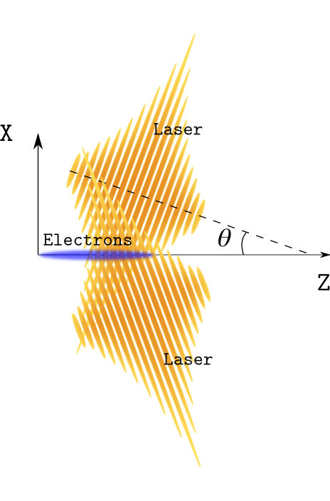
Figure 1: Optical lattice scheme

The beam of electrons travels at a relativistic velocity, $v_{b}=\sqrt{1-\gamma_{b}^{-2}}\simeq 1$, in the overlap of two identical laser pulses incident symmetrically with the angle $\theta$ (see fig. 1). The vector potential $\mathbf{a}=\mathbf{a}_{L}+\mathbf{a}_{s}$ in eq. 1 accounts for the lattice field,

$$\mathbf{a}_{L}=2a_{0}\mathbf{e}_{y}\sin(x\sin\theta)\cos(t-z\cos\theta)\,,$$ (2a)

and the signal wave $$\mathbf{a}_{s}$$, associated with the scattered radiation. This signal co-propagates with electrons:

$$\mathbf{a}_{s}=a_{s}\mathbf{e}_{y}\cos(k_{s}(t-z))\,,$$ (2b)

and its amplitude $a_{s}$ is assumed to be small, so in our analysis we retain only linear terms on $a_{s}$.

One approximation commonly used to describe the motion of the charged particles in a strong laser field, is to divide this motion into the “fast” and “slow” parts. The fast reaction of the electrons is to follow oscillations of the electromagnetic field directly. On the other hand, the particles are also driven by the period-averaged ponderomotive force, defined by the field spatial gradients. The optical lattice field in eq. 2a has the transverse gradient, which creates the ponderomotive force along $x$-axis:

$$\mathbf{F}^{(0)}=-\mathbf{e}_{x}\gamma_{b}^{-1}a_{0}^{2}\partial_{x}|\sin(x\sin\theta)|^{2}\,,$$ (3a)

and produces a series of the potential channels with the widths $$L_{x}=\pi/2\sin\theta$$.

In presence of the signal wave (2b), its interference with the lattice produces a beat-wave in the longitudinal direction. This wave acts on the electrons via the ponderomotive force:

$$\mathbf{F}^{(1)} =\mathbf{e}_{z}a_{0}a_{s}\gamma_{b}(k_{s}(1-v_{b})+v_{b}-\cos\theta)$$ (3b)

$$\sin(x\sin\theta)\sin\Big{[}(1-k_{s})t-(\cos\theta-k_{s})z\Big{]}\,.$$

which is calculated in the reference frame of electron beam (cf. gibbon:2005 ), and then translated to the laboratory system.

II.1 Unperturbed beam in the lattice

The unperturbed state of the electron beam trapped in the lattice potential is defined only by the transverse ponderomotive force eq. 3a. The characteristics of the kinetic equation (1a) in this case can be written as:

$$\frac{\mathrm{d}x}{v_{x}}=\frac{\mathrm{d}p_{x}}{F^{(0)}}\,,\quad\mathrm{d}t=\frac{\mathrm{d}z}{v_{z}}\,,$$ (4)

and they define the particles trajectories, along which the initial EDF remains constant. The first equation of eq. 4 represents the energy conservation condition,

$$p_{x}^{2}/2a_{0}^{2}+\sin^{2}(x\sin\theta)=\xi^{2}\,,$$ (5)

and, neglecting the variations of the electron Lorentz factor, we may calculate the orbits of the electrons as:

$$\sin(x\sin\theta)=\mathrm{sn}(\xi\Omega_{0}t+\Theta;\xi^{-2})\,.$$ (6)

where $\mathrm{sn}(u,m)\equiv\sin(\phi)$ is a Jacobi elliptic function defined as an inverse of elliptic integral ${u=\int_{0}^{\phi}(1-m\sin^{2}\theta)^{-1/2}\,\mathrm{d}\theta}$. Here we have also denoted a normalized excursion $\xi$, and $\Omega_{0}=\sqrt{2}a_{0}\sin\theta/\gamma_{e}$ is a frequency of the small-amplitude oscillations. The phase $\Theta$ is defined by the initial coordinates and momentum of the particle.

If $\xi<1$, the electron is trapped, and it oscillates in a channel of the optical lattice with the frequency:

$$\Omega=\cfrac{\pi\,\Omega_{0}}{2K(\xi)}\simeq\Omega_{0}\left(\cfrac{\sin\pi\xi}{\pi\xi}\right)^{1/6}\approx\Omega_{0}(1-\xi^{2}/3)\,,$$ (7)

where $K(m)=\int_{0}^{\pi/2}(1-m\sin^{2}\phi)^{-1/2}\,\mathrm{d}\phi$, is an quarter period of elliptic integral.

The first approximation in eq. 7 was previously presented in andriyash:PRSTAB13 , and its accuracy is better than 99% for $\xi<0.999$. The alternative expression (in the leftmost part of eq. 7) is derived by expanding $\sin^{2}(x\sin\theta)$ into the series, and it retains a 98% accuracy for $\xi<0.85$. The latter is more convenient for the analytical developments, and we will use it further with the electron orbits eq. 6 approximated by sinusoids. Finally, the set of electron trajectories in the $(x\,,z)$ phase-plane will read:

$$X=\Big{(}x_{0}\cos(\Omega t)+p_{x0}/(\Omega\gamma_{e})\sin(\Omega t)\Big{)}\,,$$

$$P_{x}=\Big{(}(p_{x0}\cos(\Omega t)-x_{0}\Omega\gamma_{e}\sin(\Omega t)\Big{)}\,,$$ (8)

$$Z=z_{0}+v_{z}t\,,\quad v_{z}=\mathrm{const}\,.$$

For a simple model analysis one can assume homogeneous electron distributions in the transverse phase plane, where the particles are trapped, and in the longitudinal direction, which is not affected by the lattice field. The electron distribution function in this case reads:

$$f=\frac{n_{0}}{4\sqrt{2}a_{0}\xi_{0}\delta\gamma_{b}}\,\eta\left(\xi_{0}^{2}-\xi^{2}\right)\eta(\delta\gamma-|p_{z}-p_{b}|)\,,$$ (9)

where $\eta(x)$ is a unit-step function, $n_{0}=n_{e}(x=0)$ is a maximal electron density, and $\delta\gamma$ is a longitudinal energy spread of electrons. The maximal excursion is limited by the potential scale, $\xi_{0}\leq 1$.

II.2 Interaction of the electron density perturbations and the signal electromagnetic wave

The force (3b) associated with the signal wave acts on the particles, and rearranges their longitudinal positions, thus generating the perturbation of EDF $f\to f+\delta f$. In its turn, this perturbation acts back on the signal field through the electron current along $y$-axis in the right hand side of eq. 1b. Such coupling may provide a resonant interaction between electron and electromagnetic modes resulting in their amplification or damping similarly to the stimulated Raman scattering Kruer:1988 .

During the early, linear stage of interaction, the amplitude of the signal wave and the EDF perturbations are small $a_{s}\ll a_{0}$, $\delta f\ll f$. The current $\int\mathbf{v}f\mathrm{d}\mathbf{p}$, associated with the resonant interaction in eq. 1b, includes the generating term $a_{L}\delta n/\gamma_{e}$, and the term $a_{s}n_{e}/\gamma_{e}$, which is responsible for the dispersion of the signal resulting from its interaction with the space-charge plasma waves. In the simplest case, we may neglect this dispersion as well as the diffraction of the amplified wave, therefore, assuming a plane transverse profile. Keeping only the first order resonant perturbation terms, we write the signal wave equation as:

$$\partial_{t}a_{s}=i\,\frac{a_{0}n^{*}}{\gamma_{b}k_{s}}\sin(x\sin\theta)\,,$$ (10)

where $n^{*}$ is related to the electron density perturbations as

$$\delta n=\int\delta f\mathrm{d}\mathbf{p}=\mathrm{Re}\left[n^{*}\mathrm{e}^{i(\cos\theta-k_{s})z-i(1-k_{s})t}\right]\,.$$

To study the interaction of the electromagnetic field with relativistic electrons, it is convenient to introduce the coordinates which follow the center of the electron beam $z\to z+v_{b}t$. The Doppler-shifted frequencies of the lattice and the signal wave are $\tilde{\omega}_{e}=(1-v_{b}\cos\theta)$ and $\tilde{\omega}_{s}=(1-v_{b})k_{s}$ respectively, and the interaction is resonant when $\tilde{\omega}_{e}\approx\tilde{\omega}_{s}$ (we will discuss the resonance condition in detail in section III.2). The ponderomotive force eq. 3b and the density perturbations in the moving coordinate system read:

$$F^{(1)}=\frac{a_{0}a_{s}k_{s}}{\gamma_{b}}\,\sin(x\sin\theta)\sin\Big{[}\Omega_{s}t+k_{s}z\Big{]}\,,$$

$$\delta n=\mathrm{Re}\left[n^{*}\mathrm{e}^{-i(\Omega_{s}t+k_{s}z)}\right]\,,$$ (11)

where we assumed $k_{s}\gg\cos\theta$, and $\Omega_{s}=\tilde{\omega}_{e}-\tilde{\omega}_{s}$ is a frequency of the slow oscillations of longitudinal ponderomotive force. Note that, it is the force $F^{(1)}$, which produces the modulations of electron density – the bunched structure. These modulations propagate with the velocity $-\Omega_{s}/k_{s}$, and the sign of $\Omega_{s}$ defines the propagation direction. In case of $\Omega_{s}<0$, the modulations co-propagate with the electron beam and accelerate the particles, thereby draining the energy of electromagnetic field. Otherwise, if the signal is down-shifted, $\tilde{\omega}_{s}<\tilde{\omega}_{e}$, the electrons give the energy to the wave amplifying it. In what follows, we will consider only this growing mode, always assuming $\Omega_{s}>0$.

Let us describe the dynamics of $n^{*}$ by perturbing the kinetic equation (1b) and averaging it over the lattice field period:

$$\left[\partial_{t}+v_{x}\partial_{x}+v_{z}\partial_{z}+F^{(0)}\partial_{p_{x}}\right]\delta f=-F^{(1)}\partial_{p_{z}}f\,,$$ (12)

where only the first order terms are retained. The operator in the left hand side is simply the time derivative $\mathrm{d}\delta f/\mathrm{d}t$ calculated along the trajectories (II.1). Substituting these trajectories into eq. 12 and considering the model EDF eq. 9, the integration of eq. 12 over the momenta may be simplified as:

$$n^{*}=\frac{a_{0}n_{0}k_{s}^{2}}{4\gamma^{4}\xi_{0}}\sin(x\sin\theta)\int_{-\infty}^{t}\mathrm{d}t^{\prime}a_{s}(t^{\prime})G(t^{\prime}-t)$$ (13)

where we denote $\chi=x\sin\theta$, and the function:

$$G(t)=\frac{\sin(k_{s}\delta v_{z}t)}{k_{s}\delta v_{z}}\,\int_{0}^{\xi_{0}^{2}}\;\mathrm{d}\xi^{2}\frac{\mathrm{e}^{i(\Omega-\Omega_{s})t}}{\sqrt{\xi^{2}-\sin^{2}\chi}}\,,$$

describes dynamics of the electron density perturbations driven by the ponderomotive forces. Here we have also neglected the non-resonant up-shifted mode $\exp[-i(\Omega+\Omega_{s})t]$. The longitudinal energy spread of electrons is represented here by the parameter $\delta v_{z}=\delta\gamma_{e}/\gamma_{b}^{3}$.

III Analysis of the stimulated scattering

Equations 13 and 10 describe the evolution of the coupled electron and electromagnetic perturbations. The conditions, at which the signal wave may be amplified, are defined by the dispersion properties of the electron beam mode. For simplicity, in the following analysis we will assume that electrons fill completely the lattice channel, so that $\xi_{0}=1$.

In our model, the electron mode is described by the function $G(t)$ in eq. 13. If we neglect the dependence of $\Omega$ on $\xi$, the electron mode would be harmonic and the integral in the function $G$ may be simplified as

$$B=\int_{0}^{1}\frac{\mathrm{e}^{i\Omega t}\;\mathrm{d}\xi^{2}}{\sqrt{\xi^{2}-\sin^{2}\chi}}=\mathrm{e}^{i\Omega_{0}t}\cos\chi\,.$$ (14)

The dependence of $\Omega$ on $\xi$ results in a deformation of the electron mode with respect to the $x$-coordinate. Considering the second approximation in eq. 7, one may qualitatively expect that the electron mode spectrum after averaging will depend on $x$ as $B\propto\mathrm{e}^{i\Omega^{\prime}t}$, where $\Omega^{\prime}=\Omega_{0}\left(1-\sin^{2}\chi/3\right)$. More accurately, the mode can be calculated as

$$B=\sqrt{6\pi}\;t^{-1/2}\;(C(\alpha)-iS(\alpha))\;\mathrm{e}^{i\Omega^{\prime}t}\,,$$ (15)

where $S(\alpha)$ and $C(\alpha)$ are the Fresnel integrals, and ${\alpha=\cos\chi\sqrt{2t/3\pi}}$.

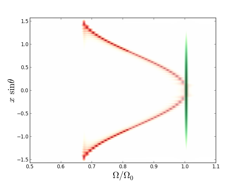
Figure 2: Electron beam mode frequency as a function of $x$-coordinate for the elliptic (red) and the harmonic (green) electron orbits.

The numerically calculated spectral-spatial map of electron beam modes given by eqs. 14 and 15 is shown in fig. 2. The deformation of the electron mode eq. 15 shown in red may increase the spectral width of the region, where the signal wave interacts resonantly with the electrons.

III.1 Interaction parameters

For the following analysis we consider the parameters which are typical for the laser accelerated electrons. The optical lattice field eq. 2a is produced by two plane waves corresponding to the pulses of a Ti:Sapphire laser with the wavelength $\lambda_{0}=800$ $\mu$m and the intensity $2.16\cdot 10^{16}$ W/cm². The incidence angles of the laser waves to the electron propagation direction are chosen to be $\theta=10^{\circ}$. A 100 pC beam of 40 MeV electrons has flat longitudinal and cylindrical transverse profiles with the duration $3.75\lambda_{0}/c$ and a radius $R_{b}=1.3\lambda_{0}$, respectively. This corresponds to the dimensionless electron density and laser amplitude $n_{0}=0.0352$ and $a_{0}=0.1$.

We also need to define the characteristics of the electron phase-space distribution. The spread of electron energies in our tests vary from the case of monoenergetic beam $\delta\gamma=0$, to a more realistic case $\delta\gamma/\gamma_{b}=0.03$. For the numerical tests, we consider a homogeneous initial spread of the electrons transverse momenta chosen to fit the trapping condition $\delta p_{x}=\sqrt{2}a_{0}$. In the physical units this corresponds to 1 mrad of rms angular divergence, and the divergence along the non-trapped $y$-direction can be assumed to be lower – 0.36 mrad.

Note that in the present analysis we do not consider the effects of the electrostatic fields. Partially this is justified by the fact that the Coulomb repelling for the relativistic beams becomes weak with higher $\gamma_{b}$. However, for a sufficiently long interaction time these effects may become important, and will be considered in future studies.

III.2 Harmonic electron mode

Let us first study an interaction with the harmonic electron mode eq. 14, assuming all electrons oscillating with the same frequency $\Omega_{0}$. In this case, the function $G$ may be calculated analytically, and eqs. 13 and 10 may be linearized with help of the Laplace transform, or by reducing eq. 13 to the differential form and performing the time-domain Fourier transform:

$$\left((\omega-\Omega_{s}+\Omega_{0})^{2}-k_{s}^{2}\delta v_{z}^{2}\right)\langle n^{*}\rangle_{\omega}=$$ (16)

$$\qquad\qquad=\langle a_{s}\rangle_{\omega}\frac{a_{0}n_{0}k_{s}^{2}}{2\gamma_{b}^{4}}\sin\chi\cos\chi\,.$$

With help of the Fourier transform we can find $\langle a_{s}\rangle_{\omega}$ from eq. 10, and substituting it to eq. 16 we obtain the dispersion equation:

$$\left((\omega-\Omega_{s}+\Omega_{0})^{2}-k_{s}^{2}\delta v_{z}^{2}\right)=\frac{a_{0}^{2}n_{0}\tilde{\omega}_{e}}{\omega\gamma^{3}}\sin^{2}\chi\cos\chi\,.$$ (17)

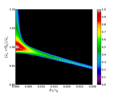
Figure 3: Normalized FEL parameter $\rho/\rho_{0}$ as a function of longitudinal temperature and signal frequency given by eq. 17. The white dashed line corresponds to the resonance condition eq. 19.

The dependence on the transverse coordinate in the right hand side of eq. 17 corresponds to the modulation of the coupling between the electron and electromagnetic modes. Physically this means that the signal wave interacts with electrons more efficiently around the coupling maxima $\chi=\pm 1/\sqrt{3}$, which tends to produce an amplified wave with a profile modulated along the $x$-axis. For the one-dimensional analysis we consider an effective mode coupling by averaging ${\langle\sin^{2}\chi\cos\chi\rangle=2/3\pi}$.

The coupling of the electromagnetic and electron modes in eq. 17 allows a resonant energy transfer from the particles to the electromagnetic field. If the solution $\omega$ has a negative imaginary part, it corresponds to the modes which grow exponentially. It is easy to see, that for a monoenergetic beam with $\delta\gamma=0$, the maximal growth occurs for $\Omega_{s}=\Omega_{0}$, and it defines the FEL parameter huang:PRSTAB2007 :

$$\rho_{0}=\left(\frac{a_{0}^{2}n_{0}}{12\pi\gamma_{b}^{3}(1-\cos\theta)^{2}}\right)^{1/3}\,,$$ (18)

which corresponds to the power gain length, ${L_{g0}=\lambda_{u}/(4\pi\sqrt{3}\rho)}$.

The finite electron energy spread suppresses the amplification and modifies its spectral structure by narrowing the resonance bandwidth and down-shifting the central wavelength as:

$$\omega_{s}\approx 2\gamma_{b}^{2}(\tilde{\omega}_{e}-\Omega_{0})/(1+2\delta\gamma/\gamma_{b})\,.$$ (19)

The maximal FEL parameter in this case decreases with the energy spread, and when $\delta\gamma/\gamma_{b}\gtrsim\rho_{0}$, it can be estimated as $\rho\approx\sqrt{2/3}(\delta\gamma/\gamma_{b})^{-1/2}\rho_{0}^{3/2}$.

The dependence of FEL parameter on the energy spread and signal frequency is presented in fig. 3, where the resonance condition eq. 19 is shown with the dashed white line. The maximal FEL parameter corresponding to the chosen interaction parameters is $\rho_{0}=4.38\cdot 10^{-3}$.

III.3 Account for the ellipticity of electron orbits

(a)	(b)

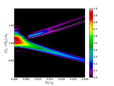
Figure 4: (a) Temporal dynamics of the signal wave as a function of its frequency calculated numerically. Color-scale is logarithmic. (b) Normalized FEL parameter $\rho/\rho_{0}$ as a function of the longitudinal temperature and the signal frequency calculated numerically for the elliptic electron mode.

For a more accurate analysis, one has to account for the dependence of electron oscillations frequency on the excursion parameter $\xi$, which may be approximately described by eq. 15. In this case, the analytical linearization of eqs. 13 and 10 would require further approximations and affect the accuracy of such description. Alternatively, these equations may be solved numerically on a finite time interval via iterations. At each iteration we integrate eqs. 13 and 10 over the time interval $(0,\tau_{0})$, and written for the normalized functions $N^{(n)}=a_{0}n^{*}/(2\gamma^{3}\tilde{\omega}_{s}\tilde{\omega}_{e})$ and $A^{(n)}=a_{s}/a_{0}$ in the following form:

$$N^{(n)}=-12\pi\rho_{0}^{3}w\sin\chi\int_{0}^{\tau}\mathrm{d}\tau^{\prime}A^{(n)}(\tau^{\prime})\tilde{G}(\tau-\tau^{\prime})\,,$$ (20a)

$$A^{(n+1)}=\frac{i}{\pi}\int_{0}^{\tau}\mathrm{d}\tau^{\prime}\int_{-\pi/2}^{\pi/2}\mathrm{d}\chi N^{(n)}\,,$$ (20b)

where $\tau=\tilde{\omega}_{e}t$, $w=\tilde{\omega}_{s}/\tilde{\omega}_{e}$, $O=\Omega_{0}/\tilde{\omega}_{e}$,

$$\tilde{G}=\frac{\sin w\delta g(\tau)}{w\delta g}\mathrm{e}^{i(1-w)\tau}B(O,\tau,\chi)\,,$$

$\delta g=2\delta\gamma/\gamma$, and the function $B$ is defined by eq. 15. Considering a small arbitrary “seed” $A^{(0)}=\mathrm{const}$, we calculate the corresponding $N^{(0)}$ from eq. 20a, and then integrate eq. 20b to obtain $A^{(1)}$.

The solution to eq. 20 can be obtained by consequently repeating this procedure till the system converges, $||A^{(n)}-A^{(n-1)}||\ll||A^{(n)}||$. In practice, this algorithm converges rapidly, and can be efficiently used for the parametric studies with complicated electron modes. This model also allows to include more effects, e.g. the divergence of the electron beam along the non-trapped direction. To do so, in the integral in eq. 20a we add the factor

$$n_{0}(t)/n_{0}(0)=\left(1+(\delta v_{y}t/\sigma_{y})^{2}\right)^{-1/2},$$ (21)

which describes a progressive decrease of electron density caused by the divergence. This modification we use later when comparing with three-dimensional numerical tests.

Let us test the numerical model for the case of the elliptic electron mode (15). In fig. 4a, we plot the evolution of the signal wave amplitude depending on the frequency for the same parameters as in fig. 3, and the energy spread $\delta\gamma/\gamma_{b}=0.01$. As expected the amplified mode grows exponentially and is down-shifted due to the electron thermal motion. One can also see excitation of the non-resonant mode up-shifted due to the electron temperature.

In fig. 4b we reproduce numerically the map of the FEL parameter as a function of the frequency and energy spread for the same parameters as in fig. 3. One may see a remarkable agreement in figs. 3 and 4b in most of the features, and the maximal FEL parameter $\rho=4.21\cdot 10^{-3}$ in this calculation agrees with $\rho_{0}$ given by eq. 18. The feature observed along,

$$\tilde{\omega}_{s}\simeq(\tilde{\omega}_{e}-\Omega_{0})/(1-2\delta\gamma/\gamma_{b})\,,$$

corresponds to a non-resonant up-shifted electron mode, and it is shown with the white dashed curve in fig. 4b. The center of the resonant region is slightly shifted, which results from the fact, that the frequency of elliptic electron oscillations $\Omega^{\prime}$ averaged over the distribution is lower than $\Omega_{0}$.

IV Simulations with the free electron laser code

The theoretical model developed in the previous section describes the amplification at the linear stage, when the main electron distribution is not affected by the growth of electron density perturbations. Therefore, such a model cannot describe the instability saturation, which occurs when a significant part of the electrons are trapped in the longitudinal potentials and stop transferring the energy to the signal wave. Near the saturation, the resonance properties of the electron beam mode (e.g. electrons energy spread) may also be significantly modified.

To account for the non-linear effects a self-consistent description is required. For this we use the particle free electron laser code PLARES andriyash:JCP2014 . In this code the relativistic electrons are presented by the macro-particles, and their unaveraged three-dimensional motion is coupled with the electromagnetic field through the spectral Maxwell solver. The code may operate in the Cartesian or axisymmetric geometries, and for the present study we use the Cartesian solver, which allows to model the asymmetric radiation profiles.

(a)	(b)

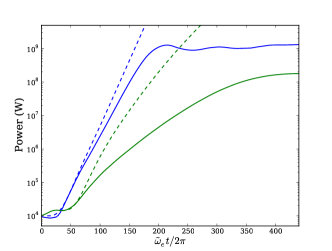
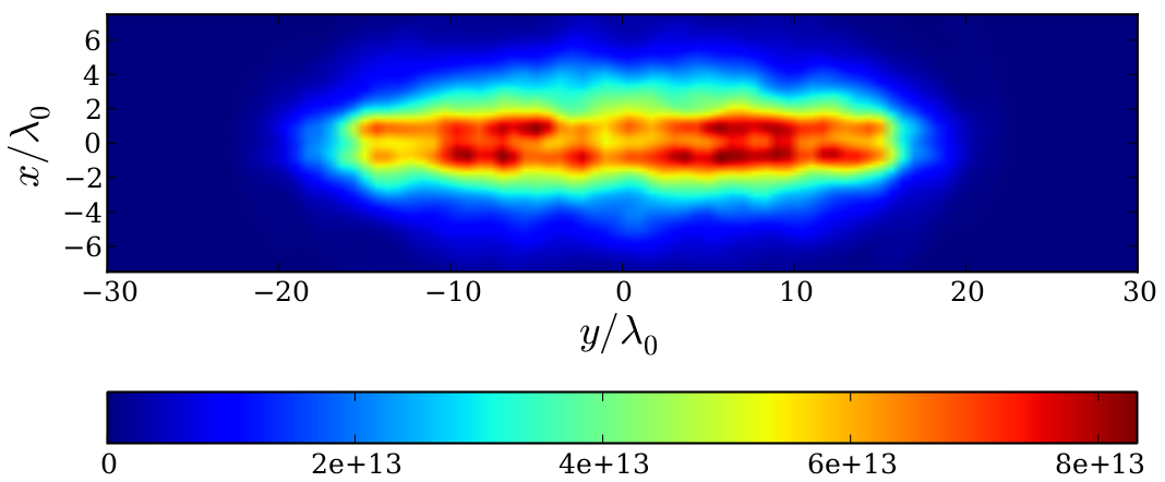
Figure 5: Steady state simulations. (a) Radiation power as a function of time for the one-dimensional (blue) and three-dimensional (green) cases modeled by PLARES (solid lines) and with help of ad hoc iterative model (20) (dashed lines). (b) The intensity profile of the X-rays at the end of the interaction in three-dimensional simulation. The colorscale is in W/cm².

The general parameters in the numerical simulations are described in section III.1. In addition, to model the injection of the electron beam into the lattice, we include a $300\lambda_{0}$ ($4.5\lambda_{y}$) linear ramp along $z$-axis. The shot-noise in the system is completely suppressed and the simulations are seeded at the resonant wavelength of 4.4 nm with a 1 kW pulse. In the three-dimensional case the transverse profiles of the seed are Gaussian and correspond to a waist of 1.7 $\mu$m.

Let us first present the steady-state simulations, where the radiation field is considered as a single-frequency infinitely long wave and it interacts with a small fraction of the electron beam in the periodic boundary conditions. This case is close to the theoretical description developed in section III, however, it accounts for the dynamics of the electron distribution and includes all related nonlinear effects. The results for the case of the monoenergetic electron beam in one-dimensional (blue solid curve) and three-dimensional (blue solid curve) simulations are presented in fig. 5a. The results of PLARES simulations are compared with the description provided by the ad hoc model (20) (dashed curves), where the three-dimensional model also accounts for the divergence eq. 21. For the one-dimensional case, we see a good agreement for the early stage of amplification, while during the main stage the growth rate is reduced by approximately 15 % due to the modification of the electron beam main state. In the three-dimensional simulation the amplification decreases even more due to the signal wave diffraction. The saturation occurs at the distances $L_{\mathrm{sat}}=1$ cm and 2 cm and reaches relatively high powers at the 1 GW and 200 MW levels for the 1D and 3D simulations, respectively.

The transverse profile of the radiation at the end of the 3D simulation is shown in fig. 5b. One may clearly observe that the resulting signal is stretched along the non-trapped direction due to the divergence of the electron beam, and is also affected by the diffraction. The intensity modulations along the $x$-axis correspond to the $\chi$ dependence of coupling between modes in eq. 17.

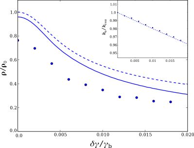
Figure 6: Dependence of the FEL parameter on the energy spread of the electrons for the analytical (dashed line) and numerical ad hoc (solid line) models (20), and in the PLARES simulations (dots). The inset shows the dependence of the normalized resonant wavenumber on the energy spread in the simulations (dots) and according to condition (19) (dashed line).

To study how the amplification is affected by electrons energy spread, we run a series of one-dimensional time-dependent simulations. The term time-dependent here means that the spectral dynamics of the signal wave is modeled, and the longitudinal profiles of the electron beam and of the seeding pulse are considered. In this model the resonance condition appears naturally corresponding to the dominant mode. The 1.5 fs seed pulse with the Gaussian longitudinal profile is used in the simulation, and its length is chosen to be much shorter than the length of the electron beam.

In fig. 6 we plot the FEL parameter as a function of $\delta\gamma/\gamma_{b}$ for the analytical model, numerical solution model and PLARES simulations. The results indicate a good qualitative agreement in the instability behavior and the demonstrate the quantitative difference of about 20 % in the values, which is also observed in fig. 5a. The central wavenumbers corresponding to the growing mode in the simulations are shown in the inset of fig. 6 and it confirms that the resonance follows the condition (19).

The results presented in this section prove a good quality of the theoretical model. The cases of more complex electron distributions can be considered in the same way. The three-dimensional analysis indicates the importance of the divergence of electron beam and the diffraction of the amplified radiation.

V Summary

We have presented a kinetic theory of the linear regime of the X-ray/XUV amplification in an electron beam, which travels in a laser-induced transverse optical lattice. The theory accounts for the energy spread and angular divergence of electron beam. For a simple realistic model of electron distribution the analytical expressions describe the amplification rate and its dependence on the longitudinal energy spread of electrons. This point has a crucial importance for the practical realizations of such a SR source. The presented results are confirmed by numerical simulations with the spectral FEL code PLARES, where the electron distribution is modeled via particle methods and the dynamics of electromagnetic field is modeled in a consistent way.

The presented analysis indicates that the amplification of the XUV light in the optical lattice is possible for the electron parameters typical of the state-of-the-art laser plasma accelerators. The account for the three-dimensional effects evidences that the electron guiding in the optical lattice plays an important role by preserving the electron flux. This opens the path for practical realizations of the optical lattice XFEL without additional components for electron focusing.

VI Acknowledgements

This work was partially supported by L’Agence Nationale de la Recherche (ANR) of France through the project LUCEL-X, and by the European Research Council through the X-Five ERC project (Contract No. 339128).

References

- (1) P. Emma et al., Nat. Phys. 4, 641 (2010).
- (2) Brian W. J. McNeil and Neil R. Thompson, Nat. Photon. 4, 814 (2010).
- (3) F. Albert et al., Phys. Rev. ST Accel. Beams 13, 070704 (2010).
- (4) K. Ta Phuoc, S. Corde, C. Thaury, V. Malka, A. Tafzi, R. C. Shah, S. Sebban, and A. Rousse, Nat. Photon. 6(5), 308 (2012)
- (5) Zhirong Huang and Kwang-Je Kim, Phys. Rev. ST Accel. Beams 10, 034801 (2007).
- (6) P. Sprangle and A. T. Drobot, J. Appl. Phys. 50(4), 2652 (1979).
- (7) A. Bacci, M. Ferrario, C. Maroli, V. Petrillo, and L. Serafini, Phys. Rev. ST Accel. Beams 9(6), 060704 (2006).
- (8) P. Sprangle, B. Hafizi, and J. R. Peñano, Phys. Rev. ST Accel. Beams 12(5), 050702 (2009).
- (9) E. Esarey, C. B. Schroeder, and W. P. Leemans, Rev. Mod. Phys. 81, 1229 (2009).
- (10) V. Malka, Phys. Plasmas 19(5), 055501 (2012).
- (11) J. Faure, C. Rechatin, A. Norlin, A. Lifschitz, Y. Glinec, and V. Malka. Nature, 444, 737–739 (2006).
- (12) Hyung Taek Kim, Ki Hong Pae, Hyuk Jin Cha, I Jong Kim, Tae Jun Yu, Jae Hee Sung, Seong Ku Lee, Tae Moon Jeong, and Jongmin Lee, Phys. Rev. Lett. 111, 165002 (2013).
- (13) W. P. Leemans, A. J. Gonsalves, H.-S. Mao, K. Nakamura, C. Benedetti, C. B. Schroeder, Cs. Tóth, J. Daniels, D. E. Mittelberger, S. S. Bulanov, J.-L. Vay, C. G. R. Geddes, and E. Esarey, Phys. Rev. Lett. 113, 245002 (2014).
- (14) H.-P. Schlenvoigt et al., Nat. Phys. 4, 130 (2008).
- (15) Matthias Fuchs et al., Nat Phys. 5, 826 (2009).
- (16) Kazuhisa Nakajima, Nat. Phys. 4, 92 (2008).
- (17) P. L. Kapitza and P. A. M. Dirac, Math. Proc. Cambridge 29(02), 297 (1933).
- (18) P. H. Bucksbaum, D. W. Schumacher, and M. Bashkansky, Phys. Rev. Lett. 61(10), 1182 (1988).
- (19) D.L. Freimund, K. Aflatooni, and H. Batelaan, Nature 413, 132 (2001).
- (20) M. V. Fedorov, K. B. Oganesyan, and A. M. Prokhorov, Appl. Phys. Lett. 53(5), 353 (1988).
- (21) S. Sepke, Y.Y. Lau, J.P. Holloway, and D. Umstadter, Phys. Rev. E 72(2), 026501 (2005).
- (22) Ph. Balcou, Eur. Phys. J. D 59, 525 (2010).
- (23) I. A. Andriyash, E. d’Humières, V. T. Tikhonchuk, and Ph. Balcou, Phys. Rev. Lett. 109, 244802 (2012).
- (24) I.A. Andriyash, Ph. Balcou, and V.T. Tikhonchuk, Eur. Phys. J. D 65, 533 (2011).
- (25) E.N. Frolov, A.V. Dik, and S.B. Dabagov, Nucl. Instrum. Meth. B 309(0), 157 (2013).
- (26) I. A. Andriyash, E. d’Humières, V. T. Tikhonchuk, and Ph. Balcou, Phys. Rev. ST Accel. Beams 16, 100703 (2013).
- (27) A.D. Debus, M. Bussmann, M. Siebold, A. Jochmann, U. Schramm, T.E. Cowan, and R. Sauerbrey, Appl. Phys. B 100(1), 61 (2010).
- (28) K. Steiniger, R. Widera, R. Pausch, A. Debus, M. Bussmann, and U. Schramm. Nucl. Instrum. Meth. A 740(0), 147 (2014).
- (29) I.A. Andriyash, R. Lehe, and V. Malka, J. Comput. Phys. 282(0), 397 (2015).
- (30) Paul Gibbon, Short Pulse Laser Interactions with Matter: An Introduction. Imperial College Press, 2005.
- (31) William Kruer, The Physics of Laser Plasma Interactions. Westview Press, 1988.