The Exclusion Process: A paradigm for non-equilibrium behaviour
Abstract
In these lectures, we shall present some remarkable results that have been obtained for systems far from equilibrium during the last two decades. We shall put a special emphasis on the concept of large deviation functions that provide us with a unified description of many physical situations. These functions are expected to play, for systems far from equilibrium, a role akin to that of the thermodynamic potentials. These concepts will be illustrated by exact solutions of the Asymmetric Exclusion Process, a paradigm for non-equilibrium statistical physics.
A system at mechanical and at thermal equilibrium obeys the principles of thermodynamics that are embodied in the laws of equilibrium statistical mechanics. The fundamental property is that a system, consisting of a huge number of microscopic degrees of freedom, can be described at equilibrium by only a few macroscopic parameters, called state variables. The values of these parameters can be determined by optimizing a potential function (such as the entropy, the free energy, the Gibbs free energy…) chosen according to the external constraints imposed upon the system. The connection between the macroscopic description and the microscopic scale is obtained through Boltzmann’s formula (or one of its variants). Consider, for example, a system system at thermal equilibrium with a reservoir at temperature . Its thermodynamical properties are encoded by Boltzmann-Gibbs canonical law:
where the Partition Function Z is related to the thermodynamic Free Energy F via
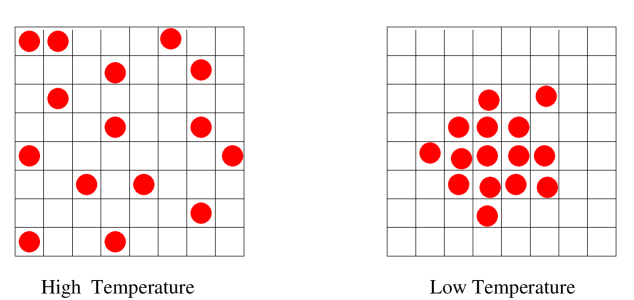
This expression (which is a consequence of Boltzmann’s formula ) shows that the determination of the thermodynamic potentials can be expressed as a combinatorial (or counting) problem, which of course, can be extremely complex. Nevertheless, equilibrium statistical physics provides us with a well-defined prescription to analyse thermodynamic systems: an explicit formula for the canonical law is given; this defines a probability measure on the configuration space of the system; statistical properties of observables (mean-values, fluctuations) can be calculated by performing averages with respect to this probability measure. The paradigm of equilibrium statistical physics is the Ising Model (see Figure 1). It was solved in two dimensions by L. Onsager (1944). We emphasize that equilibrium statistical mechanics predicts macroscopic fluctuations (typically Gaussian) that are out of reach of classical thermodynamics: the paradigm of such fluctuations is the Brownian Motion.
For systems far from equilibrium, a theory that would generalize the formalism of equilibrium statistical mechanics to time-dependent processes is not yet available. However, although the theory is far from being complete, substantial progress has been made, particularly during the last twenty years. One line of research consists in exploring structural properties of non-equilibrium systems: this endeavour has led to celebrated results such as Fluctuation Theorems that generalize Einstein’s fluctuation relation and linear response theory. Another strategy, inspired from the research devoted to the Ising model, is to gain insight into non-equilibrium physics from analytical studies and from exact solutions of some special models. In the field of non-equilibrium statistical mechanics, the Asymmetric Simple Exclusion Process (ASEP) is reaching the status of a paradigm.
In these lecture notes, we shall first review equilibrium properties in Section I. Using Markov processes, we shall give a dynamical picture of equilibrium in Section I.1. Then we shall introduce the detailed balance condition and explain how it is related to time reversal (Section I.2). This will allow us to give a precise definition of the concept of ‘equilibrium’ from a dynamical point of view.
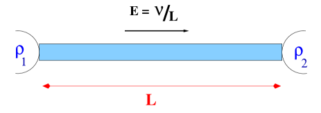
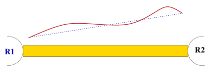
The study of non-equilibrium processes will begin in Section II. We shall use as a leitmotiv for non-equilibrium, the picture of rod (or pipe) in contact with two reservoirs at different temperatures, or at different electrical (chemical) potentials (see Figure 8). This simple picture will allow us to formulate some of the basic questions that have to be answered in order to understand non-equilibrium physics. The current theory of non-equilibrium processes requires the use of some mathematical tools, such as large-deviation functions, that are introduced, through various examples (Independent Bernoulli variables, random walk…), in Section II.1; in particular, we explain how the thermodynamic Free Energy is connected to the large deviations of the density profile of a gas enclosed in a vessel. In Section II.2, we show the relations between the large-deviation function and cumulants of a random variable. Section II.3 is devoted to the very important concept of generalized detailed balance, a fundamental remnant of the time-reversal invariance of physics, that prevails even in situations far from equilibrium. Then, in Section II.4, the Fluctuation Theorem is derived for Markov system that obey generalized detailed balance.
From Section III on, these lectures focus on the Asymmetric Exclusion Process (ASEP) and on some of the techniques developed in the last twenty years to derive exact solutions for this model and its variants. After a brief presentation of the model and of some of its simple properties (Sections III.1 to III.3), we apply the Mean-Field approximation to derive the hydrodynamic behaviour in Section III.4; in particular, this technique is illustrated on the Lebowitz-Janowsky blockage model, a fascinating problem that has so far eluded an exact solution. Finally, in Section III.5, the celebrated exact calculation of the steady state of the ASEP with open boundaries, using the Matrix Representation Method, is described.
Section IV contains a crash-course on the Bethe Ansatz. We believe that the ASEP on a periodic ring, is the simplest model to learn how to apply this very important method. We try to explain the various steps that lead to the Bethe Equations in Section IV.1. These equations are analysed in the special TASEP case in Section IV.2.
We are now ready to calculate large deviation functions for non-equilibrium problems: this is the goal of Section V. Our aim is to derive large deviations of the stationary current for the pipe picture, modelled by the ASEP. This is done first for the periodic case (ASEP on a ring) in Section V.1, then for the open system in contact with two reservoirs (Section V.2). The similarities between the two solutions are emphasized. Exact formulae for cumulants and for the large deviation functions are given. This Section is the most advanced part of the course and represents the synthesis of the concepts and techniques that were developed in earlier sections. Detailed calculations are not given and can be found in recent research papers.
The last section is devoted to concluding remarks and is followed by the Bibliography. We emphasize that these lecture notes are not intended to be a review paper. Therefore, the bibliography is rather succinct and is restricted to some of the books, review papers or articles that were used while preparing this course. More precise references can be found easily from these sources. Our major influences in preparing these lectures come from the review of B. Derrida DerrReview and from the book of P. L. Krapivsky, S. Redner and E. Ben-Naim PaulK .
I Dynamical Properties of the Equilibrium State
The average macroscopic properties of systems at thermodynamic equilibrium are independent of time. However, one should not think that thermodynamic equilibrium means absence of dynamical behaviour: at the microscopic scale, the system keeps on evolving from one micro-state to another. This never-ending motion manifests itself as fluctuations at the macroscopic scale, the most celebrated example being the Brownian Motion. However, one crucial feature of a system at thermodynamic equilibrium is the absence of currents in the system: there is no macroscopic transport of matter, charge, energy, momentum, spin or whatsoever within the system or between the system and its environment. This is a very fundamental property, first stated by Onsager, that stems from the time-reversal symmetry of the microscopic equations of motion. This property is true both for classical and quantum dynamics.
I.1 Markovian dynamical models
We want to describe the evolution of a complex system consisting of a very large number of interacting degrees of freedom. In full rigour, one should write the -body (quantum) Hamiltonian that incorporates the full evolution of the system under consideration. However, it is often useful to consider effective dynamical descriptions that are obtained, for example, by coarse-graining the phase-space of the system or by integrating-out fast modes. In the following, the models we shall study will follow classical Markovian dynamics and we shall give a short presentation of Markov systems. The interested reader can find more details, in particular about the underlying assumptions that lead to Markov dynamics, in e.g. the book by N. G. Van Kampen VanKampen . We also emphasize that many properties that we shall discuss here can be generalized to other dynamical systems.
The classical Markov processes that we shall study here will be fully specified by a (usually finite or numerable) set of microstates . At a given time , the system can be found in one its microstates. The evolution of the system is specified by the following rule: Between and , the system can jump from a configuration to a configuration . It is assumed that the transition rate from to does not depend on the previous history of the system: this is the crucial Markov hypothesis in which short time correlations are neglected. The rate of transition per unit time will be denoted by (or equivalently, by Note that this rate may vary with time and depend explicitly on . This case will not be considered in the present lectures. To summarize, the Markov dynamics is specified by the following rules:
These dynamical rules can be illustrated by a network in the configuration space (see Figure 2): the nodes of the graph are the microstates and oriented-edges, weighted by the Markov rates represent possible transitions between configurations.
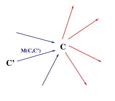
For a system with Markov dynamics, one can define , the probability of being in the micro-state at time . This probability measure varies with time: its evolution is governed by the Master equation, given by
| (1) |
This equation is fundamental. To derive it, one must take into account all possible transitions between time and that involve a given configuration . There are two types of moves: (i) transitions into coming from a different configuration ; (ii) transitions out of towards a different configuration . The moves (i) and (ii) contribute with a different sign to the change of the probability of occupying between time and . Note that the Master equation can well be interpreted as a flux-balance equation on the network of Figure 2.
The way we have encoded the transition rates naturally suggests that the Master Equation can be rewritten in a Matrix form. Indeed, reinterpreting the rate as matrix-elements and defining the diagonal term
| (2) |
allows us to rewrite Equation (1) as
| (3) |
We emphasize that the diagonal term is a negative number: it represents minus the rate of leaving the configuration . This leads to an important property: the sum of each column of identically vanishes. This property guaranties, by simple algebra, that the total probability is conserved: (the initial probability distribution being normalized).
Note that there is a formal analogy between Markov systems and quantum dynamics: the Markov operator plays the role of a quantum Hamiltonian. However, does not have to be a symmetric or Hermitian matrix (and is not, in general).
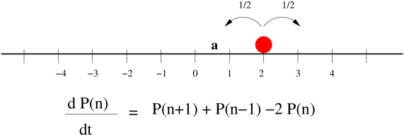
There are numerous examples of Markov processes in statistical physics. The paradigm is certainly the simple symmetric random walk on a discrete lattice (see Figure 3). Here, the configurations are the lattice sites and the transition rates are constant and uniform (i.e. translation-invariant). The corresponding Markov equation is the discrete Laplace equation on the lattice.
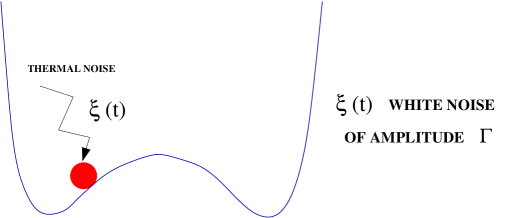
Another important example is given by Langevin dynamics (see Figure 4). It was originally invented by Paul Langevin as mechanical model for the Brownian Motion but stochastic dynamics has become a widely studied subject, that allows for instance to model the effects of noise in mechanical and electric devices. The basic idea is to incorporate a random force that represents thermal noise into classical Newtonian dynamics:
Here is a Gaussian white noise of amplitude .
The state of a particle is a point in phase-space, i.e a configuration is specified by the position and the velocity (or momentum) of the particle (the set of possible configurations is continuous and non-enumerable). The corresponding Markov equation for the probability distribution function , of being at with velocity , is known as the Fokker-Planck equation:
The role of the Markov matrix is played by the Fokker-Planck operator . There are many formal similarities between the Fokker-Planck equation and the discrete Markov dynamics given by (3); however, subtle mathematical issues can arise in the case of a continuous configuration space that require the use of functional analysis.
Both Markov and Fokker-Planck dynamics are mathematical models, that can be defined and studied without any specific reference to physical principles. However, to be physically relevant, these dynamics should be connected to the laws of thermodynamics and statistical physics. In particular, one can impose that the steady state of these equations is an equilibrium-state: in other words, the stationary probability distribution must be identical to the Boltzmann-Gibbs canonical law.
For a discrete Markov dynamics (3), this condition reads
This is a set of global constraints on the rates, which is sometimes called the ‘global balance’ condition.
Similarly, in the Langevin case, one imposes that the invariant measure of phase-space is given by
Writing that this formula is the stationary solution of the Fokker-Planck equation, one observes that this fixes the the noise-amplitude as a function of temperature
This is in essence the reasoning followed by Langevin in his study of the Free Brownian Motion (for which the external potential vanishes ). Substituting the value of in the corresponding Fokker-Planck equation leads to
Multiplying both sides of this equation by and integrating over phase-space allows us to show that
Using Stokes’ formula for the friction-coefficient (coefficient of the linearized force felt by a sphere of radius , dragged at velocity , in a liquid of viscosity ), leads to the celebrated formula of Einstein (1905) for the diffusion constant of the Brownian Motion, in terms of the Avogadro Number.
I.2 Time-reversal and Detailed Balance
We now discuss a fundamental characteristic of equilibrium dynamics that was first investigated by L. Onsager. Again, the property discovered by Onsager is a very general one. We shall present it here on Markov dynamics. The master equation (1) can be written in the following manner
where we have introduced the local probability current between and (See Figure 5).
When the stationary state is reached, we know that the right-hand side of this equation must vanish. However, equilibrium is a very particular stationary state: at equilibrium the microscopic dynamics of the system is time-reversible. This symmetry property implies that all the local currents vanish separately (Onsager):
| (4) |
This is the detailed balance equation. We emphasize that detailed balance is a very strong property goes beyond the laws of classical thermodynamics.
We shall now explain the mathematical relation between detailed balance and time-reversal. The main-idea is to use the transition rates to construct a probability measure on time-trajectories of the system.
The two important mathematical properties we shall use are the following:
1. Probability of remaining in during a time interval :
2. Probability of going from to during :
Relation 1 can be derived by calculating the probability of staying in the same configuration between and and integrating over . Relation 2 is simply the definition of the transition rates in a Markov process.
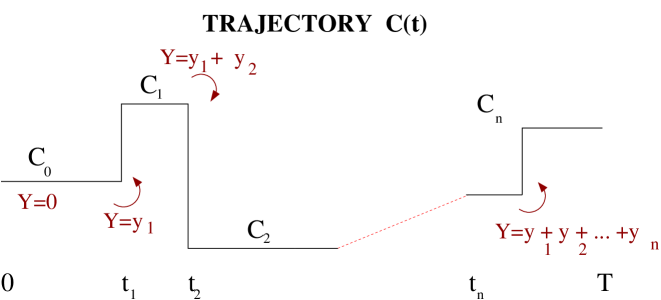
Let us now consider a ‘history’ of the system between the initial time 0 and the final . During this interval of time, the system follows a trajectory: it begins with a configuration , then at a date it jumps into configuration , stays there till and jumps to and so on. This special trajectory, denoted by is depicted in Figure 6.
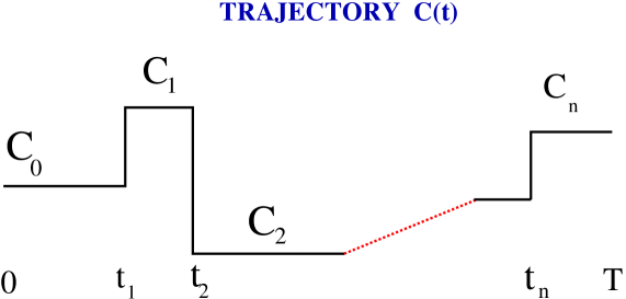
Using the relations 1 and 2 above, we can calculate the weight of this specific trajectory , i.e the probability of observing , in the equilibrium state. The only extra ingredient we need to include is the fact that the initial condition at is chosen according to the equilibrium measure. We thus have
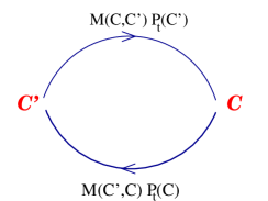
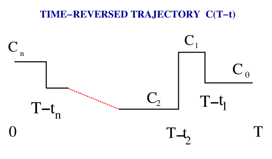
For any given trajectory , a time-reversed trajectory can be defined as . This is a bona-fide history of the system (see Figure 7) and one can calculate the probability of observing it:
If we now calculate the ratio of these two probabilities i.e. the ratio of the probability observing a given history by that of observing the reversed history , we obtain the ratio between the probabilities of forward and backward trajectories:
| (5) |
Using recursively the detailed balance condition:
and zipping it through the previous result leads us to the following remarkable identity
Hence, detailed balance implies that the dynamics is time reversible. The converse property is true: if we want that a dynamics to be time-reversal invariant, then the detailed balance relation must be satisfied (consider simply a history in which there occurs a single transition between two configurations and ).
To conclude, the detailed balance relation is a profound property of the equilibrium state that reflects time-reversal invariance of the dynamics. This relation is now taken as a definition for the concept of equilibrium: a stationary state is an equilibrium state if and only if detailed balance is satisfied.
II Nonequilibrium Processes
In Nature, many systems are far from thermodynamic equilibrium and keep on exchanging matter, energy, information with their surroundings. There is no general conceptual framework to study such systems.
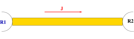
A basic example of a nonequilibrium process is a conductor, or a pipe, in contact with two reservoirs at different temperatures, or electrical or chemical potential. In the stationary state, a non-vanishing steady-state current will flow from the reservoir at higher potential towards the one at lower potential. This current clearly breaks time reversal invariance. In the vicinity of equilibrium, linear response theories allow us to predict the statistical behaviour of this current and to derive analytically the response coefficients (conductance, susceptibilities) from the knowledge of equilibrium fluctuations. However, one may wonder if a general microscopic theory, not obtained by a perturbative expansion in the vicinity of equilibrium, may be constructed. At present no such framework exists. However, in the last two decades, important progress and convincing proposals for a general description of non-equilibrium statistical mechanics have been made. We shall describe some of these theories in these lectures. Our main inspiration in this section is the two review papers by B. Derrida DerrReview ; DCairns .
For the moment being, we use the ‘pipe model’ (see Figure 8) as a paradigmatic illustration of stationary non-equilibrium behaviour and let us formulate some very basic questions:
-
•
What are the relevant macroscopic parameters? How many macroscopic observables should we include to have a fair description of the system?
-
•
Which functions describe the state of a system? Can the stationary state be derived by optimizing a potential?
-
•
Do Universal Laws exist? Can one define Universality Classes for systems out of equilibrium? Are there some general equations of state?
-
•
Can one postulate a general form for the microscopic measure that would generalize the Gibbs-Boltzmann canonical Law?
-
•
What do the statistical properties of the current in the stationary state look like (In particular, are the current fluctuations Brownian-like)?
II.1 Large Deviations and Rare Events
Large Deviation Functions (LDFs) are important mathematical objects, used in probability theory, that are becoming widely used in statistical physics. Large deviation functions are used to quantify rare events that, typically, have exponentially vanishing probabilities. We shall introduce this concept through an elementary example. A very useful review on large deviations has recently been written by H. Touchette Touchette .
Let be independent binary variables, , with probability (resp. Their sum is denoted by . We know, from the Law of Large Numbers that almost surely. Besides, the Central Limit Theorem tells us that the fluctuations of the sum are of the order . More precisely, converges towards a Normalized Gaussian Law.
One may ask a more refined question: how fast is the convergence implied by the Law of Large Numbers? In other words, what does the probability that assumes a non-typical value look like when ? For the example, we consider, elementary combinatorics shows that for , in the large limit, we have
where the positive function vanishes for . This is an elementary example of a large deviation behaviour. The function is a called a rate function or a large deviation function. It encodes the probability of rare events. A simple application of Stirling’s formula yields
We have discussed a very specific example but large deviations appear in many different contexts. We now consider an asymmetric random walker on a one-dimensional lattice with anisotropic hopping rates to neighbouring sites, given by and (see Figure 9). The average speed of the walker is given by : If is the (random) position of the walker at time we have for
We can define a large deviation function by the following relation:
valid in the limit of large times.

This function can be calculated explicitly. It is given by:
Note that
-
•
is a positive function that vanishes at .
-
•
is convex.
-
•
-
•
Using the definition of the large deviation function, we observe that, in the long time limit, the previous identity implies
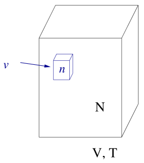
Our third example is closer to physics. Let us consider a gas, at thermodynamic equilibrium at temperature T, consisting of molecules enclosed in a vessel of total volume . The average density is . We wish to probe local density fluctuations. We consider an imaginary volume , containing a large number of molecules but remaining much smaller than the total volume, i.e. such that . Counting the number of molecules in will give us an empirical density (see Figure 10). Clearly, for large enough the empirical density will be very close to and typical fluctuations will scale as . What is the probability that significantly deviates from ?
The probability of observing large fluctuations again satisfies a large deviation behaviour:
In order to determine , we must count the fraction of the configurations of the gas in which there are particles in the small volume and particles in the rest of the volume . Suppose that the interactions of the gas molecules are local. Then, neglecting surface effects, this number is given by
Finally, we use that by definition, where is the inverse temperature and is the free energy per unit volume and perform an expansion for . This leads to
We emphasize that this large deviation function is very closely related to the thermodynamic Free Energy.
A more general question would be the large deviation of a density profile. Suppose we fully cover the large box with small boxes. What is the probability of observing an empirical density in the first box, in the second box etc…? Here again, we can show that a large deviation principle is satisfied:
where the large deviation function depends on variables. A reasoning similar to the one above allows us to show that
Taking the infinite volume limit, we obtain
If now, we let the number of boxes go to infinity, then the question we are asking is the probability of observing a given density profile in the big volume . For , the large deviation function becomes a functional of the density profile:
being, as above, the free energy per unit volume. We conclude that the Free Energy of Thermodynamics could have been defined ab initio as a large deviation function. More generally, all thermodynamic potentials can be realized as large deviation functions.
However, the concept of large deviations does not pertain to equilibrium. Large deviation functions can be introduced for very general processes, even far from equilibrium. They are positive functions that attain their minimum for when their argument takes the typical stationary variable. These remarks suggest that these functions may be used as potentials in non-equilibrium statistical mechanics.
II.2 Large Deviations and Cumulants
Let be a variable that satisfies a large deviation principle in the limit :
where the large deviation function is positive and vanishes at .
Another way to encode the statistics of is to study its moment-generating function, defined as the average value Expanding with respect of , we get
where denotes the -th cumulant of .
From the large deviation principle, we can show the following behaviour:
| (6) |
This implies that all all cumulants of grow linearly with time and their values are given by the successive derivatives of . Moreover, the cumulant generating function and the large deviation function are related by Legendre transform. This can be seen by using the saddle-point method:
From this relation we conclude that,
| (7) |
In the following examples, we shall often calculate first and then determine by a Legendre transformation.
II.3 Generalized Detailed Balance
We have shown that detailed balance is a fingerprint of equilibrium. Conversely, out of equilibrium, time reversibility and detailed balance are broken. A priori, one could imagine that any arbitrary Markov operator could represent a physical system far from equilibrium. This is not the case: the fundamental laws of physics are time-reversible (leaving apart some aspects of weak-interaction). It is only after a coarse-graining procedure, when non-relevant degrees of freedom are integrated out, that the resulting effective dynamics appears to be irreversible for the restricted degrees of freedom we are interested in and for the space and time scales that we are considering. Nevertheless, whatever coarse-grained description is chosen at a macroscopic scale, a signature of this fundamental time-reversibility of physics must remain. In other words, in order to have a sound physical model, even very far from equilibrium, detailed balance can not be violated in an arbitrary manner: there is a ‘natural way’ of generalizing detailed balance. We shall investigate here what happens to detailed balance for a system connected to unbalanced reservoirs (as in the pipe paradigm).
We first reformulate the equilibrium detailed balance, to make generalizations more transparent.
The Equilibrium Case:
A system is a thermal equilibrium with a reservoir at satisfies the detailed balance with respect to the Boltzmann weights. Equation (4) becomes
| (8) |
Equivalently, defining which represents the energy exchanged between the system and the reservoir at a transition from to , the above equation becomes
| (9) |
where we have added an index to keep track of the exchanges of energy.
The Non-Equilibrium Case:
Consider now a system in contact with two reservoirs and at and . Suppose that during an elementary step of the process, the system can exchange energy (or matter…) with the first reservoir and with the second one. Then, generalized detailed balance is given by
| (10) |
where for . This equation can be obtained by the following physical reasoning. Consider the global system : this is an isolated system, its total energy is conserved by the dynamics. Considered as a whole, the global system is governed by a reversible dynamics and in the infinite time limit it will reach the microcanonical measure. Besides, its dynamics must satisfy detailed balance with respect to this microcanonical measure. This condition is expressed as
where and are the entropies of the reservoirs (i..e the logarithms of the phase-space volumes). Using the fact that the reservoirs are at well-defined temperatures and that energy exchanges with the system are small (i.e. ), we can expand the entropy variations of each reservoir and this leads us to Equation (10).
We give now a more abstract formulation of generalized detailed balance in which energy exchanges with the reservoirs are replaced by the flux of an arbitrary quantity (it can be a mass, a charge, an entropy…). Let us suppose that during an elementary transition from to between and , the observable , is incremented by :
We shall also assume that is odd with respect to time-reversal, i.e. by time reversal, the increment changes its sign:
A generalized detailed balance relation with respect to will be satisfied if there exists a constant such that the transition rates satisfy
| (11) |
This formula can be further extended by considering multiple exchanges of various quantities between different reservoirs: the statement of generalized detailed balance becomes
II.4 The Fluctuation Theorem
We shall now discuss a very important property of systems out of equilibrium, known as the Fluctuation Theorem. This relation was derived by G. Gallavotti and E. D. G. Cohen Gallavotti . Here, we follow the proof of the Fluctuation Theorem for valid for Markov processes that was given by Lebowitz and Spohn LeboSpohn A crucial emphasis is put on the generalized detailed balance relation.
The idea is to investigate how the generalized detailed balance equation (11) modifies the reasoning of in section I.2, where we showed that detailed balance and time reversibility are equivalent.
As in section I.2, we consider a trajectory (or history) of the system between time 0 and . Now, for each jump between two configurations, we also keep track of the increment in the quantity for which the generalized detailed balance equation (11) is valid (see Figure 11).
As in section I.2, we compute the ratio between the probabilities of forward and backward trajectories: equation (5) is not modified (it is true for any Markov process). But, now, we simplify this ratio by using the generalized detailed balance equation (11). We obtain
| (12) |
where represents the total quantity of transferred when the system follows the trajectory between 0 and .
Here, the ratio between the forward and backward probabilities is different from unity. The dynamics is not reversible anymore and the breaking of time-reversal is precisely quantified by the total flux of . Recall that is odd, under time reversal. Hence, we have
It is now useful to define the auxiliary quantity:
The quantity is again odd w.r.t. time-reversal and it satisfies
or, equivalently,
| (13) |
Summing over all possible histories between time 0 and , leads us to
Interpreting both sides as average values, we obtain
| (14) |
This is the statement of the Fluctuation Theorem in Laplace space, for the auxiliary variable . The quantities and grow with time, linearly in general. Their difference remains, generically, bounded (beware: this could be untrue for some specific systems where ‘condensation’ in some specific configurations occurs. We assume here this does not happen). This implies that, in the long time limit, and have the same statistical behaviour and therefore
A Legendre transform yields the Gallavotti-Cohen Fluctuation Theorem for the large deviation function
| (16) |
Using the large deviation principle, this identity implies
| (17) |
This relation is the generic way of stating the Fluctuation Theorem. It compares the probability of occurrence of an event (for example, a total flux of charge, or energy or entropy) with that of the opposite event. This relation is true far from equilibrium. It has been proved rigorously in various contexts (chaotic systems, Markov/Langevin dynamics…).
Remark: In the multiple variable case, we would obtain for the multi-cumulant generating function
Or equivalently, for the large deviation function,
III The Exclusion Process
A fruitful strategy to gain insight into non-equilibrium physics is to extract as much information as possible from analytical studies and from exact solutions of some special models. Building a simple representation for complex phenomena is a common procedure in physics, leading to the emergence of paradigmatic systems: the harmonic oscillator, the random walker, the Ising model. All these ‘beautiful models’ often display wonderful mathematical structures Baxter .
In the field of non-equilibrium statistical mechanics, the Asymmetric Simple Exclusion Process (ASEP) is reaching the status of such a paradigm. The ASEP consists of particles on a lattice, that hop from a site to its immediate neighbours, and satisfy the exclusion condition (there is at most one particle per site). Therefore, a jump is allowed only if the target site is empty. Physically, the exclusion constraint mimics short-range interactions amongst particles. Besides, in order to drive this lattice gas out of equilibrium, non-vanishing currents must be established in the system. This can be achieved by various means: by starting from non-uniform initial conditions, by coupling the system to external reservoirs that drive currents through the system (transport of particles, energy, heat) or by introducing some intrinsic bias in the dynamics that favours motion in a privileged direction. Thus, each particle is an asymmetric random walker that interacts with the other and drifts steadily along the direction of an external driving force.
From Figure 12, it can be seen that the ASEP on a finite lattice, in contact with two reservoirs, is an idealization of the paradigmatic pipe picture of Figure 8 that we have been constantly discussing.
To summarize, the ASEP is a minimal model to study non-equilibrium behaviour. It is simple enough to allow analytical studies, however it contains the necessary ingredients for the emergence of a non-trivial phenomenology:
-
•
ASYMMETRIC: The external driving breaks detailed-balance and creates a stationary current in the system. The model exhibits a non-equilibrium stationary state.
-
•
EXCLUSION: The hard core-interaction implies that there is at most 1 particle per site. The ASEP is a genuine N-body problem.
-
•
PROCESS: The dynamics is stochastic and Markovian: there is no underlying Hamiltonian.
III.1 Definition of the Exclusion Process
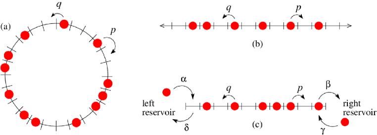
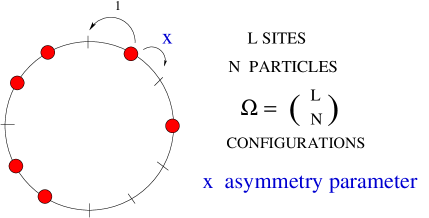
The ASEP is a Markov process, consisting of particles located on a discrete lattice that evolves in continuous time. We shall consider only the case when the underlying lattice is one dimensional. The stochastic evolution rules are the following: at time a particle located at a site in the bulk of the system jumps, in the interval between and , with probability to the next neighbouring site if this site is empty (exclusion rule) and with probability to the site if this site is empty. The scalars and are parameters of the system; by rescaling time, one often takes and arbitrary. (Another commonly used rescaling is ). In the totally asymmetric exclusion process (TASEP) the jumps are totally biased in one direction ( or ). On the other hand, the symmetric exclusion process (SEP) corresponds to the choice . The physics and the phenomenology of the ASEP are extremely sensitive to the boundary conditions. We shall mainly discuss three types of boundary conditions (see Figure 13):
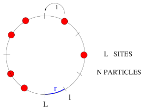
(i) The periodic system: the exclusion process is defined on a one dimensional lattice with sites (sites and are identical) and particles. Note that the dynamics conserves the total number of particles
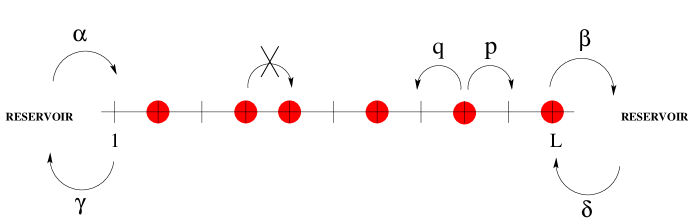
(ii) The finite one-dimensional lattice of sites with open boundaries. Here, the site number (entrance site) and site number play a special role. Site 1 interacts with the left reservoir as follows: if site 1 is empty, a particle can enter with rate whereas if it is occupied it can become vacant with rate . Similarly, the interactions with the right reservoir are as follows: if site is empty, a particle can enter the system with rate and if is occupied, the particle can leave the system with rate . The entrance and exit rates represent the coupling of the finite system with infinite reservoirs which are at different potentials and are located at the boundaries. In the special TASEP case, : particles are injected by the left reservoir, they hop in the right direction only and can leave the system from the site number to the right reservoir.
(iii) The ASEP can also be defined on the infinite one-dimensional lattice. Here, the boundaries are sent to . Boundary conditions are here of a different kind: the infinite system remains always sensitive to the configuration it started from. Therefore, when studying the ASEP on the infinite lattice one must carefully specify the initial configuration (or statistical set of configurations) the dynamics has begun with.
III.2 Various Incarnations of the ASEP
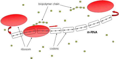
Due to its simplicity, the ASEP has been introduced and used in various contexts. It was first proposed as a prototype to describe the dynamics of ribosomes along RNA MGP (see Figure 14). In the mathematical literature, Brownian processes with hard-core interactions were defined by Spitzer who coined the name exclusion process. The ASEP also describes transport in low-dimensional systems with strong geometrical constraints such as macromolecules transiting through capillary vessels, anisotropic conductors, or quantum dots where electrons hop to vacant locations and repel each other via Coulomb interaction. Very popular modern applications of the exclusion process include molecular motors that transport proteins along filaments inside the cells and, of course, ASEP and its variants are ubiquitous in discrete models of traffic flow Andreas2 . More realistic models that are relevant for applications will not described further: we refer the reader to the review paper CKZ that puts emphasis on biophysical applications.
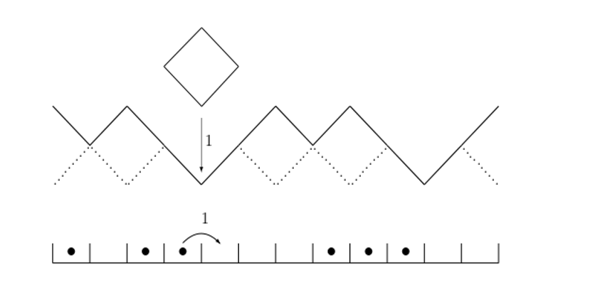
Another feature of ASEP is its relation with growth processes and in particular to the Kardar-Parisi-Zhang equation in one-dimension (see Figure 15). A classic review on this subject is HHZ . The relation between the exclusion process and KPZ has lead recently to superb mathematical developments: we refer the readers to recent reviews Sasamoto ; Kriecherbauer for details and references.
More generally, the ASEP belongs to the class of driven diffusive systems defined by Katz, Lebowitz and Spohn in 1984 KLS (see Zia for a review). We emphasize that the ASEP is defined through dynamical rules: there is no energy associated with a microscopic configuration. More generally, the kinetic point of view seems to be a promising and fruitful approach to non-equilibrium systems.
We emphasize that there are very many variants of the fundamental ASEP: the dynamical rules can be modified (discrete-time dynamics, sequential or parallel updates, shuffle updates); one can introduce local defects in the model by modifying the dynamics on some specific bonds; it is possible to consider different types of particles with different hopping rates; one can also consider quenched or dynamical disorder in the lattice; the lattice geometry itself can be changed (two-lane models, ASEP defined on a stripe, on a network etc…). All these alterations drastically modify the outcome of the dynamics and require specific methods to be investigated. Literally hundreds of works have been devoted to the ASEP and its variants during the last fifteen years. Here, we shall focus only on the homogeneous case with the three ideal types of boundary conditions discussed above and present some of the mathematical methods that have been developed for these three ideal cases.
III.3 Basis Properties of ASEP
The evolution of the ASEP is encoded in the Markov operator . For a finite-size system, the Markov operator is a matrix; for the infinite system is an operator and its precise definition needs more elaborate mathematical tools Spohn91 . Unless stated otherwise, we shall focus here on the technically simpler case of a finite configuration space of size and the infinite system limit is obtained formally by taking . An important feature of the ASEP on a finite lattice is ergodicity: any configuration can evolve to any other one in a finite number of steps. This property insures that the Perron-Frobenius theorem holds true (see, for example VanKampen ). This implies that the Markov matrix contains the value 0 as a non-degenerate eigenvalue and that all other eigenvalues have a strictly negative real part. The physical interpretation of the spectrum of is the following: the right eigenvector associated with the eigenvalue 0 corresponds to the stationary state (or steady-state) of the dynamics. Because all non-zero eigenvalues have a strictly negative real part, the corresponding eigenmodes of are relaxation states: the relaxation time is given by and the imaginary part of leads to oscillations.
We emphasize that from the mathematical point of view, the operator encodes all the required data of the dynamics and any ‘physical’ questions that one may ask about the system ultimately refers to some property of . We shall now list some fundamental issues that may arise:
-
•
Once the dynamics is properly defined, the basic question is to determine the steady-state of the system i.e., the eigenvector of with eigenvalue 0. Given a configuration , the value of the component is the stationary weight (or measure) of in the steady-state, i.e., it represents the frequency of occurrence of in the stationary state.
-
•
The knowledge of the vector is similar to knowing the Gibbs-Boltzmann canonical law in equilibrium statistical mechanics. From one can determine steady-state properties and all equal-time steady-state correlations. Some important questions are: what is the mean occupation of a given site ? What does the most likely density profile, given by the function , look like? Can one calculate density-density correlation functions between different sites? What is the probability of occurrence of a density profile that differs significantly from the most likely one (this probability is called the large deviation of the density profile)?
-
•
The ASEP, being a non-equilibrium system, carries a finite, non-zero, steady-state current . The value of this current is an important physical observable of the model. The dependence of on the external parameters of the system can allow to define different phases of the system.
-
•
Fluctuations in the steady-state: the stationary state is a dynamical state in which the system constantly evolves from one micro-state to another. This microscopic evolution induces macroscopic fluctuations (which are the equivalent of the Gaussian Brownian fluctuations at equilibrium). How can one characterize steady-state fluctuations? Are they necessarily Gaussian? How are they related to the linear response of the system to small perturbations in the vicinity of the steady-state? These issues can be tackled by considering tagged-particle dynamics, anomalous diffusion, time-dependent perturbations of the dynamical rules etc…
-
•
The existence of a current in the stationary state corresponds to the physical transport of some extensive quantity (mass, charge, energy) through the system. The total quantity transported during a (long) period of time in the steady-state is a random quantity. We know that the mean value of is given by but there are fluctuations. More specifically, in the long time limit, the distribution of the random variable represents exceptional fluctuations of the mean-current (known as large deviations): this is an important observable that quantifies the transport properties of the system.
-
•
The way a system relaxes to its stationary state is also an important characteristic of the system. The typical relaxation time of the ASEP scales with the size of the system as , where is the dynamical exponent. The value of is related to the spectral gap of the Markov matrix , i.e., to the real-part of its largest non-vanishing eigenvalue. For a diffusive system, one has . For the ASEP with periodic boundary condition, an exact calculation leads to . More generally, the transitory state of the model can be probed using correlation functions at different times.
-
•
The matrix is generally a non-symmetric matrix and, therefore, its right eigenvectors differ from its left eigenvectors. For instance, a right eigenvector corresponding to the eigenvalue is defined as
(18) Knowing the spectrum of conveys a lot of information about the dynamics. There are analytical techniques, such as the Bethe Ansatz, that allow us to diagonalize in some specific cases. Because is a real matrix, its eigenvalues (and eigenvectors) are either real numbers or complex conjugate pairs.
-
•
Solving analytically the master equation would allow us to calculate exactly the evolution of the system. A challenging goal is to determine the finite-time Green function (or transition probability) , the probability for the system to be in configuration at time , knowing that the initial configuration at time was . The knowledge of the transition probability, together with the Markov property, allows us in principle to calculate all the correlation functions of the system.
The following sections are devoted to explaining some analytical techniques that have been developed to answer some of these issues for the ASEP.
III.4 Mean-Field analysis of the ASEP
Before discussing exact techniques to solve the dynamics of the ASEP, we want to explain the mean-field approach. In many physically important cases with inhomogeneities or more complex dynamical rules, mean-field calculations are the only available technique and they often lead to sound results that can be checked and compared with numerical experiments.
III.4.1 Burgers Equation in the Hydrodynamic Limit.
In the limit of large systems, it is natural to look for a continuous description of the model. Finding an accurate hydrodynamic model for interacting particle processes is a difficult and important problem. Here, we present a naive approach that reveals the relation between the ASEP and Burgers equation.
We recall that the binary variable characterizes if site is empty or occupied. The average value satisfies the following equation:
For : 1-point averages couple to 2-points averages etc… A hierarchy of differential equations is generated (cf BBGKY). This set of coupled equations can not be solved in general. The mean-field approach can be viewed as a technique for closing the hierarchy. For the ASEP, the procedure is quite simple. We sketch it below: Define the continuous space variable . and the limit
Define a smooth local density by .
Rescale the rates: and
Mean-field assumption: write the 2-points averages as products of 1-point averages.
After carrying out this program leads to, after a diffusive rescaling of time to the following partial differential equation
| (19) |
This is the Burgers equation with viscosity.
To resume, starting from the microscopic level, we have defined a local density and a local current that depend on macroscopic space-time variables (diffusive scaling) in the limit of weak asymmetry (see Figure 16). Then, we have found that the typical evolution of the system is given by the hydrodynamic behaviour:
We have explained how to obtain this equation in a ‘hand-waving’ manner. However, the result is mathematically correct: it can be proved rigorously that the continuous limit of the weakly-asymmetric ASEP is described, on average, by this equation. The proof is a major mathematical achievement.
Had we kept a finite asymmetry: , the same procedure (with ballistic time-rescaling) would have led us to the inviscid limit of Burgers equation:
This equation is a textbook example of a PDF that generates shocks, even if the initial condition is smooth. A natural question that arises is whether these shocks an artefact of the hydrodynamic limit or do they genuinely exist at the microscopic level. The following model, invented by J. L. Lebowitz and S. A. Janowsky sheds light on this issue.
III.4.2 A worked-out example: The Lebowitz-Janowsky model
The Lebowitz-Janowsky model describes the formation of shocks at the microscopic scale JL1 . This is very simple model, but it has not been solved exactly. It will provide us with a good illustration of mean-field methods.
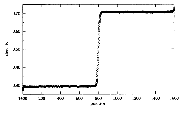
The simplest version of Lebowitz-Janowsky model is a TASEP on a periodic ring with one defective bound: through that bound (say the bond between site and site 1) the jump rate is given by whereas through all the other bonds, the jump rates are equal to 1. For (which is the most interesting case), we have a slow bond, i.e. a constriction, that may prevent the flow of particles through and generate a ’traffic-jam’. This is indeed what is going to happen: for any given density , there is a critical value such that for a separation will occur between a dense phase before the slow bond and a sparse phase after that bond.
The blockage model can be analysed by elementary mean-field considerations. Through a ‘normal’ bond the current is exactly given by In the stationary state, this current is uniform . Far from the blockage and from the shock region,the density is approximately uniform (as numerical simulations show, see Figure 17). Thus, using a mean-field assumption we can write
where and are the values of the density plateaux on both sides of the slow bond. This relation leads to two possible solutions:
Either the density is uniform everywhere, i.e.,
Or we have different densities on the sides that make a shock. Then, necessarily:
To find the values of the density plateaux, we calculate the mean-field current right at the defective bond:
(This is a strong approximation that neglects correlations through the slow bond.) We now have enough equations to obtain
To conclude the analysis, we must find the condition for the existence of the shock: when do we have and when ? We must use the conservation of the number of particles. Let be the position of the shock, then we have i.e., dividing by :
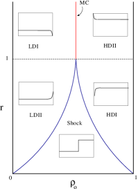
This relation defines the phase boundary between the uniform and the shock phases. It can be rewritten in a more elegant manner as follows:
From this equation, we observe, in particular, that a shock will always appear for as soon as . The full phase diagram of the system is drawn in Figure 18. Numerical simulations seem to support this phase diagram. However, no exact proof is available. Besides, using an improved mean field analysis, the form of the shock can be calculated. However, the results do not coincide with simulations. The exact solution of the Lebowitz-Janowsky model is a celebrated open problem in this field (see JL1 for references and some recent progress).
 |
 |
III.5 The Steady State of the open ASEP: The Matrix Ansatz
There does not exist a method to calculate the stationary measure for a non-equilibrium interacting model. After briefly describing the stationary state of the ASEP with periodic boundary conditions and of the ASEP on the infinite line, we shall focus on the ASEP with open boundaries.
For the ASEP on a ring the steady state is uniform: all configurations have the same probability. The proof is elementary: for any configuration the number of states it can reach to by an elementary move is equal to the total number of configurations that can evolve into it.
For the exclusion process on an infinite line, the stationary measures have been fully studied and classified Spohn91 . There are two one-parameter families of invariant measures: one family, denoted by , is a product of local Bernoulli measures of constant density , where each site is occupied with probability ; the other family is discrete and is concentrated on a countable subset of configurations. For the TASEP, this second family corresponds to blocking measures, which are point-mass measures concentrated on step-like configurations (i.e., configurations where all sites to the left of a given site are empty and all sites to the right of are occupied).
We now consider the case of the ASEP on a finite and open lattice with open boundaries. For convenience, we rescale the time so that forward jumps occur with rate 1 and backward jumps with rate . This scalar is called the asymmetry parameter.
Here, the mean-field method gives a reasonably good approximation. However, it is not exact for a finite system. There are notable deviations in the density profile (i.e. the function where is the average density at site ). Moreover, fluctuations and rare events are not well accounted for by mean-field. We shall now explain a method to obtain the exact stationary measure for the ASEP with open boundaries. This technique, known as the Matrix Representation Method, was developed in DEHP . Since that seminal paper, it has become a very important tool to investigate non-equilibrium models. The review written by R. A. Blythe and M. R. Evans allows one to learn the Matrix Representation Method for the ASEP and other models and also to find many references MartinRev2 .
A configuration can be represented by a string of length , , where is the binary occupation variable of the site (i.e. or 0 if the site is occupied or empty). The idea is to associate with each configuration , the following matrix element:
| (20) |
The operators and , the vectors and satisfy
| (21) |
The claim is that if the algebraic relations (21) are satisfied then, the matrix element (20), duly normalized, is the stationary weight of the configuration . Note that the normalization constant is where
This algebra encodes combinatorial recursion relations between systems of different sizes. Generically, the representations of this quadratic algebra are infinite dimensional (-deformed oscillators).
| (26) |
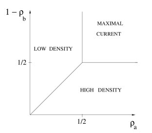
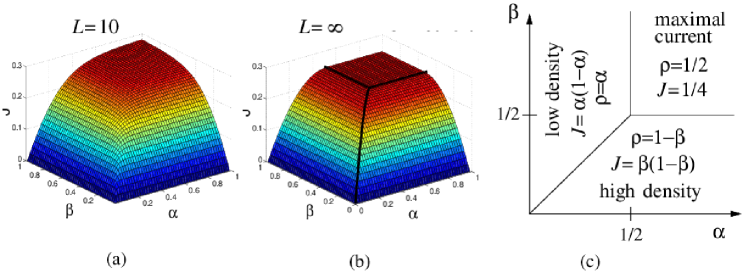
The matrix Ansatz allows one to calculate Stationary State Properties (currents, correlations, fluctuations) and to derive the Phase Diagram in the infinite size limit. There are three phases, determined by the values of and that represent effective densities of the left and the right reservoir, respectively. The precise formulae for these effective densities for the general ASEP model were found by T. Sasamoto:
| where | |||||
| where | (27) |
In the TASEP case and , the algebra simplifies and reduces to
For this case, many calculations can be performed in rather simple manner. In particular, the average stationary current is found to be
In fact, the Matrix Ansatz gives access to all equal time correlations in the steady-state. For example, the density profile:
or even Multi-body correlations:
The expressions look formal but it is possible to derive explicit formulae: either by using purely combinatorial/algebraic techniques or via a specific representation (e.g., can be chosen as a discrete Laplacian). For example, we have
The TASEP phase diagram is shown in Figure 20.
For the general ASEP case, results can be derived through more elaborate methods involving orthogonal polynomials, as shown by T. Sasamoto (1999). More details and precise references can again be found in the review of R. Blythe and M. R. Evans MartinRev2 .
The Matrix Ansatz is an efficient tool to investigate the stationary state. However, it does not allow us to access to time-depend properties: how does the system relax to its stationary state? Can we calculate fluctuations of history-dependent observables (such as the total number of particles exchanged between the two reservoirs during a certain amount of time)?
IV The Bethe Ansatz for the Exclusion Process
In order to investigate the behaviour of the system which is not stationary, the spectrum of the Markov matrix is needed. For an arbitrary stochastic system, the evolution operator can not be diagonalized. However, the ASEP belongs to a very special class of models: it is integrable and it can be solved using the Bethe Ansatz as first noticed by D. Dhar in 1987. Indeed, the Markov matrix that encodes the stochastic dynamics of the ASEP can be rewritten in terms of Pauli matrices; in the absence of a driving field, the symmetric exclusion process can be mapped exactly into the Heisenberg spin chain. The asymmetry due to a non-zero external driving field breaks the left/right symmetry and the ASEP becomes equivalent to a non-Hermitian spin chain of the XXZ type with boundary terms that preserve the integrable character of the model. The ASEP can also be mapped into a six vertex model. These mappings suggest the use of the Bethe Ansatz to derive spectral information about the evolution operator, such as the spectral gap Gwa ; ogkmrev and large deviation function.
Let us apply the Bethe Ansatz to the ASEP on a ring. A configuration can be characterized by the positions of the particles on the ring, with . With this representation, the eigenvalue equation (18) becomes
| (28) | |||||
where the sum are restricted over the indexes such that and over the indexes such that these conditions ensure that the corresponding jumps are allowed.
We observe that equation (28) is akin to a discrete Laplacian on a -dimensional lattice: the major difference is that the terms corresponding to forbidden jumps are absent. Nevertheless, this suggests that a trial solution (Ansatz in German) in the form of plane waves may be useful. This is precisely the idea underlying the Bethe Ansatz. In the following we shall give an elementary introduction to this technique which is used in very many different areas of theoretical physics. Originally, H. Bethe developed it to study the Heisenberg spin chain model of quantum magnetism. The ASEP is the one of the simplest systems to learn the Bethe Ansatz.
IV.1 Bethe Ansatz for ASEP: a crash-course
Our aim is to solve the linear eigenvalue problem (28) which corresponds to the relaxation modes of the ASEP with particles on a ring of sites. We shall study some special cases with small values of in order to unveil the general structure of the solution.
The 1 particle case:
For , equation (28) reads
| (29) |
with and where periodicity is assumed
| (30) |
Equation (29) is simply a linear recursion of order 2 that is solved as
| (31) |
where are the two roots of the characteristic equation
| (32) |
The periodicity condition imposes that at least one of the two characteristic values is a -th root of unity (Note that because both of them can not be roots of unity as soon as ). The general solution is, finally,
| (33) |
The solution is therefore a simple plane wave with momentum and with eigenvalue
| (34) |
The 2 particles case:
The case where two particles are present is more interesting because when the particles are located on adjacent sites the exclusion effect plays a role. Indeed, the general eigenvalue equation (28) can be split into two different cases:
The Generic case: here and are separated by at least one empty site:
| (35) | |||||
The (special) adjacency case: , some jumps are forbidden and the eigenvalue equation reduces to:
| (36) |
This equation differs from the generic equation (35) in which we substitute : there are missing terms. An equivalent way to take into account the adjacency case is to impose that the generic equation (35) is valid for all values of and and add to it the following cancellation boundary condition:
| (37) |
We now examine how these equations can be solved. In the generic case particles behave totally independently (i.e., they do not interact). The solution of the generic equation (35) can therefore be written as a product of plane waves , with the eigenvalue
| (38) |
However, the simple product solution can not be the full answer: indeed the cancellation condition for the adjacency case (37) has to be satisfied also. The first crucial observation, following H. Bethe, is that the eigenvalue , given in (38) is invariant by the permutation . In other words, there are two plane waves and with the same eigenvalue which has a two-fold degeneracy; the full eigenfunction corresponding to can thus be written as
| (39) |
where the amplitudes and are yet arbitrary. The second key step is to understand that these amplitudes can now be chosen to fulfil the adjacency cancellation condition: if we substitute the expression (39) in equation (37), we obtain the relation
| (40) |
The eigenfunction (39) is therefore determined, but for an overall multiplicative constant. We now implement the periodicity condition that takes into account the fact that the system is defined on a ring. This constraint can be written as follows for
| (41) |
This relation plays the role of a quantification condition for the scalars and that we shall call hereafter the Bethe roots. Indeed, if we impose the condition that the expression (39) satisfies equation (41) for all generic values of the positions and we obtain new relations between the amplitudes:
| (42) |
Comparing equations (40) and (42) leads to a set of algebraic equations obeyed by the Bethe roots and :
| (43) | |||||
| (44) |
These equations are known as the Bethe Ansatz Equations. Finding the spectrum of the Matrix for two particles on a ring of size is reduced to solving these two coupled polynomial equations of degree of order with unknowns and . Surely, this still remains a very challenging task but the Bethe equations are explicit and very symmetric. Besides, we emphasize that the size of the matrix (and the degree of its characteristic polynomial) is of order .
The 3 particles case:
We are now ready to consider the case . For a system containing three particles, located at , the generic equation, valid when the particles are well separated, can readily be written using equation (28). But now, the special adjacency cases are more complicated:
(i) Two particles are next to each other and the third one is far apart; such a setting is called a 2-body collision and the boundary condition that results is identical to the one obtained for the case . There are now two equations that correspond to the cases and :
| (45) | |||||
| (46) |
We emphasize again that these equations are identical to equation (37) because the third particle, located far apart, is simply a spectator ( is a spectator in the first equation; in the second one).
(ii) There can be 3-body collisions, in which the three particles are adjacent, with . The resulting boundary condition is then given by
| (47) |
The fundamental remark is that 3-body collisions do not lead to an independent new constraint. Indeed, equation (47) is simply a linear combination of the constraints (45) and (46) imposed by the 2-body collisions. To be precise: equation (47) is the sum of equation (45), with the substitutions and , and of equation (46) with and . Therefore, it is sufficient to fulfil the 2-body constraints because then the 3-body conditions are automatically satisfied. The fact that 3-body collisions decompose or ’factorize’ into 2-body collisions is the crucial property that lies at the very heart of the Bethe Ansatz. If it were not true, the ASEP would not be exactly solvable or ’integrable’.
For , the plane wave is a solution of the generic equation with the eigenvalue
| (48) |
However, such a single plane wave does not satisfy the boundary conditions (45) and (46). Here again we note that the eigenvalue is invariant under the permutations of and . There are 6 such permutations, that belong to the permutation group of 3 objects. The Bethe wave-function is therefore written as a sum of the 6 plane waves, corresponding to the same eigenvalue , with unknown amplitudes:
| (49) | |||||
| (50) |
The 6 amplitudes are uniquely and unambiguously determined (up to an overall multiplicative constant) by the 2-body collision constraints. It is therefore absolutely crucial that 3-body collisions do not bring additional independent constraints that the Bethe wave function could not satisfy. We strongly encourage the reader to perform the calculations (which are very similar to the case) of the amplitude-ratios.
Finally, the Bethe roots , and are quantized through the periodicity condition
| (51) |
for . This condition leads to the Bethe Ansatz equations (the equations for general are given below).
The general case:
Finally, we briefly discuss the general case . Here one can have -body collisions with . However, all multi-body collisions ’factorize’ into 2-body collisions and ASEP can be diagonalized using the Bethe Wave Function
| (52) |
where is the permutation group of objects. The amplitudes are fixed (up to an overall multiplicative constant) by the 2-body collision constraints. The corresponding eigenvalue is given by
| (53) |
The periodicity condition
| (54) |
leads to a set of algebraic equations satisfied by the Bethe roots . The Bethe Ansatz equations are given by
| (55) |
for . The last equation is obtained by using the asymmetry parameter .
The Bethe Ansatz thus provides us with a set of coupled algebraic equations of degree of order (Recall that the size of the matrix is of order , when ). Although the Bethe equations are highly non-linear, a huge variety of methods have been developed to analyse them.
We remark that for the Bethe equations are the same as the ones derived by H. Bethe in 1931. Indeed, the symmetric exclusion process is identical to the isotropic Heisenberg spin chain.
IV.2 Analysis of the Bethe Equations for the TASEP
For TASEP, the Bethe equations take a simpler form: making the change of variable , these equations become
Note that the r.h.s. is a constant independent of : There is an effective DECOUPLING. The corresponding eigenvalue is
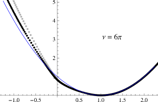
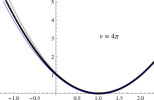
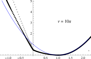
For a fixed value of the r.h.s. the roots lie on curves that satisfy
where is the density (see Figure 21).
The fact that the Bethe equations can be reduced to an effective single-variable polynomial suggests the following self-consistent procedure for solving them:
-
For any given value of , SOLVE The roots are located on Cassini Ovals
-
CHOOSE roots amongst the available roots, with a choice set
-
SOLVE the self-consistent equation where
-
DEDUCE from the value of , the ’s and the energy corresponding to the choice set :
This program can be carried through to calculate the spectral gap of the Markov matrix , which amounts to calculating the eigenvalue with largest strictly negative real part. For a density , one obtains for the TASEP
The first excited state consists of a pair of conjugate complex numbers when is different from 1/2. The real part of describes the relaxation towards the stationary state: we find that the largest relaxation time scales as with the dynamical exponent Dhar ; Gwa . This value agrees with the dynamical exponent of the one-dimensional Kardar-Parisi-Zhang equation that belongs to the same universality class as ASEP (see the review of Halpin-Healy and Zhang 1995 HHZ and Sasamoto ; Kriecherbauer for recent developments.). The imaginary part of represents the relaxation oscillations and scales as ; these oscillations correspond to a kinematic travelling wave that propagates with the group velocity . For the partially asymmetric case (), the Bethe equations do not decouple and analytical results are much harder to obtain (see ogkmrev for references).
V Large Deviation far from Equilibrium
We now return to our basic picture of a conducting pipe between two unbalanced reservoirs (Figure 8) and formulate some questions involving the concept of large deviations. Using the ASEP as a paradigm, we shall explain how the tools developed above (Bethe Ansatz, Matrix Representation) can help us to give mathematically precise answers to these problems.
1. In the pipe model, a steady-state is reached with a non-vanishing constant current and a stationary density profile . Typically, this density profile will be linear (as seen by using Fick’s phenomenological law). We have seen above that for a system in equilibrium (i.e. when the two reservoirs are at the same potential) the large deviations of the density profile are determined by the free energy. A similar question can be raised in the non-equilibrium stationary state: What is the probability of observing an atypical density profile in the steady state (see Figure 22)? More precisely, assuming a large deviation behaviour,
what does the functional look like in this non-equilibrium system?
For the ASEP, the answer to this question was given by B. Derrida, J. Lebowitz E. Speer in 2002. These authors calculated the probability of observing an atypical density profile in the steady state of the ASEP, starting from the exact microscopic solution of the exclusion process, with the help of the Matrix Ansatz. For the symmetric exclusion process (which corresponds to a discrete version of Fick’s law), the large deviation functional is given by
where and satisfies
It is important to note that this functional is non-local as soon as and that it is is NOT identical to the one given by assuming local equilibrium.
2. A similar problem can be raised about the current fluctuations. Let us call the total charge (or time-integrated current) transported through the system between time 0 and time , then
where is the average steady-state current. However, the observable is a random variable, that may take non-typical values. Its fluctuations obey a large deviation principle:
where is the large deviation function of the total current. Note that is positive, vanishes at and is convex (in general). A natural question is to derive a mathematical formula . We shall describe below the exact solution for the ASEP.
V.1 Current Fluctuations far from equilibrium on a periodic ring
We consider in this section the case of a periodic ring and study the statistics of the total displacement of all the particles in the system time 0 and time . Because the system is finite, this total displacement is proportional to the time integrated current. The ASEP on a periodic ring is drawn again in Figure 23, For convenience, time has been rescaled so that forward jumps occur with rate 1, whereas backward jumps occur with rate .
Thus, here, will represent the total distance covered by all the particles between time 0 and time and is the joint probability of being in the configuration at time and having . The evolution equation of is:
| (56) |
Using the generating function
| (57) |
the evolution equation becomes
| (58) |
This equation is similar to the original Markov equation for the probability distribution but now the original Markov matrix is deformed by a jump-counting fugacity into (which is not a Markov matrix in general), given by
| (59) |
In the long time limit, , the behaviour of is dominated by the largest eigenvalue and one can write
| (60) |
Thus, in the long time limit, the function is the generating function of the cumulants of the total current . But is also the dominant eigenvalue of the matrix . Therefore, the current statistics has been traded into an eigenvalue problem. Fortunately, the deformed matrix can still be diagonalized by the Bethe Ansatz. In fact, a small modification of the calculations described in Section IV leads to the following Bethe Ansatz equations
| (61) |
where the asymmetry parameter is the ratio of the rates of backward to forward jumps. The eigenvalues of are given by
| (62) |
The cumulant generating function corresponds to the largest eigenvalue.
V.1.1 The periodic TASEP Case
For the TASEP, , and the Bethe equations (61) again decouple and can be studied by using the procedure outlined in Section IV.2. This case was completely solved by B. Derrida and J. L. Lebowitz in 1998 DLeb . These authors calculated by Bethe Ansatz to all orders in . More precisely, they obtained the following representation of the function in terms of an auxiliary parameter :
| (65) | |||||
| (68) |
These expressions allow to calculate the cumulants of , for example the mean-current and the diffusion constant :
| (69) | |||||
| (70) |
When , with a fixed density and , the large deviation function can be written in the following scaling form:
| (71) |
with
| for | (72) | ||||
| for | (73) |
This large deviation function is not a quadratic polynomial, even in the vicinity of the steady state. Moreover, the shape of this function is skew: it decays as the exponential of a power law with an exponent for and with an exponent for .
V.1.2 The periodic ASEP: Functional Bethe Ansatz
In the general case , the Bethe Ansatz equations do not decouple and a procedure for solving them was lacking. For example, it did not even seem possible to extract from the Bethe equations (61) a formula for the mean stationary current (which can be obtained very easily by other means from the fact that the stationary measure is uniform). This problem was solved in a few steps and the complete solution was given by S. Prolhac in 2010 Sylvain4
The periodic ASEP can be analysed by rewriting the Bethe Ansatz as a functional equation and restating it as a purely algebraic problem, as we shall now explain. First, we perform the following change of variables,
| (74) |
In terms of the variables the Bethe equations read
| (75) |
Here again the equations do not decouple as soon as . However, these equations are now built from first order monomials in the ’s and they are symmetrical in these variables. This observation suggests to introduce an auxiliary variable that plays the same role with respect to all the ’s and allows to define the auxiliary equation:
| (76) |
This equation, in which is the unknown, and the ’s are parameters, can be rewritten as a polynomial equation:
| (77) |
Because the Bethe equations (75) imply that for , the polynomial , defined as
| (78) |
must divide the polynomial . Now, if we examine closely the expression of , we observe that the factors that contain the ’s inside the products over can be written in terms of . Therefore, we conclude that DIVIDES Equivalently, there exists a polynomial such that
| (79) |
This functional equation is equivalent to the Bethe Ansatz equations (it is also known as Baxter’s TQ equation). It can be used to determine the polynomial of degree that vanishes at the Bethe roots. In the present case, equation (79) can be solved perturbatively w.r.t. to any desired order. Knowing perturbatively an expansion of is derived, leading to the cumulants of the current and to the large deviation function. For example, this method allows to calculate the following cumulants of the total current:
Mean Current :
Diffusion Constant :
In the limit of a large system size, , with asymmetry parameter and with a fixed value of , the diffusion constant assumes a simple expression
Third cumulant: the Skewness measures the non-Gaussian character of the fluctuations. An exact combinatorial expression of the third moment, valid for any values of , and , was calculated by S. Prolhac in 2008. It is given by
For , and keeping fixed, this formula becomes
This shows that the fluctuations display a non-Gaussian behaviour. We remark that for the TASEP limit is recovered:
V.1.3 The weakly asymmetric limit
In this section, we make some remarks specific to the weakly asymmetric case, for which the asymmetry parameter scales as in the limit of large system sizes . In this case, we also need to rescale the fugacity parameter as and the following asymptotic formula for the cumulant generating function can be derived
| (80) | |||||
| (81) |
and where the ’s are Bernoulli Numbers. We observe that the leading order (in ) is quadratic in and describes Gaussian fluctuations. It is only in the subleading correction (in ) that the non-Gaussian character arises. We observe that the series that defines the function has a finite radius of convergence and that has a singularity for . Thus, non-analyticities appear in as soon as
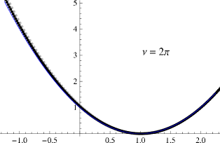
By Legendre transform, non-analyticities also occur in the large deviation function . At half-filling, the singularity appears at as can be seen in Figure 24. For the leading behaviour of is quadratic (corresponding to Gaussian fluctuations) and is given by
| (82) |
For , the series expansions (80) and (81) break down and the large deviation function becomes non-quadratic even at leading order. This phase transition was predicted by T. Bodineau and B. Derrida using macroscopic fluctuation theory (see Bodineau for a general discussion). One can observe in Figure 24 that for , the large deviation function becomes non-quadratic and develops a kink at a special value of the total current .
V.1.4 The general structure of the solution
A systematic expansion procedure that completely solves the problem to all orders and yields exact expressions for all the cumulants of the current, for an arbitrary value of the asymmetry parameter , was carried out by S. Prolhac in Sylvain4 .
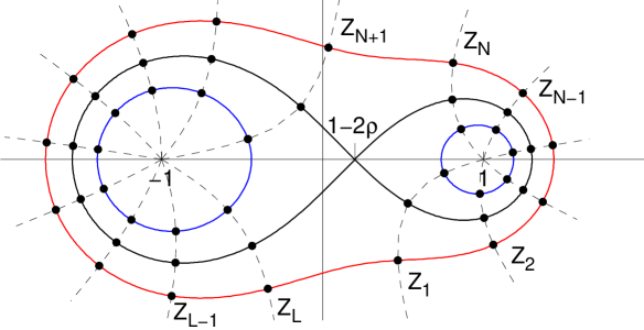
Using the functional Bethe Ansatz, S. Prolhac derived a parametric representation of the cumulant generating function similar to the one given for the TASEP in equations (65) and (68),
| (83) |
where and can be expressed as residues of a complex function :
It can be shown that and are combinatorial factors that are enumerate to some tree structures. To find these numbers, we need the functions . These functions can be embodied into a generating function defined as
| (84) |
This function encodes the full information about the statistics of the current: if we know how to determine it, the problem is solved.
It can be proved that is the solution of the following functional Bethe equation:
| (85) |
| (86) |
where the kernel is given by
| (87) |
Equations (85, 86 and 87) determine the unknown function . They are the core of the problem’s solution. Using them, a closed expansion of w.r.t. was derived. This expansion, valid for any finite values of , and , can be used to study the large system size limit with various scalings of the asymmetry. Various regimes were found and the corresponding expressions for the cumulants were fully worked out:
-
•
For , the model falls into the Edward-Wilkinson universality class.
-
•
The range , where is a finite number, defines the weakly asymmetric regime (to be discussed below).
-
•
The intermediate regime, corresponding to , exhibits a specific scaling behaviour that, to our knowledge, can not be represented by a continuous stochastic equation.
-
•
For the system is in the strongly asymmetric regime.
-
•
The range corresponds to the KPZ universality class, which contains the TASEP.
V.2 Open System with reservoirs
Finally, we can explain how to calculate the large deviation of the current in the open ASEP in contact with two reservoirs Gorissen . Now, the observable counts the total number of particles exchanged between the system and the left reservoir between times and . During a time interval , increases by 1 if a particle enters at site 1 (at rate ), it decreases by if a particle exits from 1 (at rate ) and is unchanged if no particle exchange with the left reservoir has occurred during .
We know that converges towards the average current when . We wish to determine the large deviation function associated with or, equivalently, its cumulant generating function, that we recall is defined by
The function can be calculated by the Matrix Ansatz method. The solution obtained has structure very similar to the one obtained in Equations (85, 86 and 87) for the periodic case. For arbitrary values of and , and for any system size the parametric representation of is given by
The coefficients and are given by contour integrals in the complex plane:
where the complex contour encircles 0, , for [ were defined in equation (27)]. Here again, there exists an auxiliary function that contains the full information about the statistics of the current. The functional equation for is given by
| (88) |
being the same operator defined in equations (86) and (87). But the function is now given by
where we use the notation . This function, related to Askey-Wilson polynomials, was used by T. Sasamoto in his study of the stationary state of the ASEP with open boundaries (see MartinRev2 for references).
If we specialize these formulae to the special TASEP case with non-zero rates equal to unity , the expression becomes rather explicit. The parametric representation of the cumulant generating function is given by
By eliminating recursively in terms of in second equation and substituting in the first one, we can calculate the first few cumulants of the current:
-
•
Mean Value :
-
•
Variance :
-
•
Skewness :
For large systems:
More generally, in the limit of large system sizes, the asymptotic behaviour of can be carried out, for the general ASEP, in the different phases. In the Low Density (and High Density) Phases, the large deviation function, obtained after a Legendre transform, takes a particularly simple form:
where the current is parametrized as
The exact expressions can also be compared with numerical results obtained by the Density Matrix Renormalization Group technique.
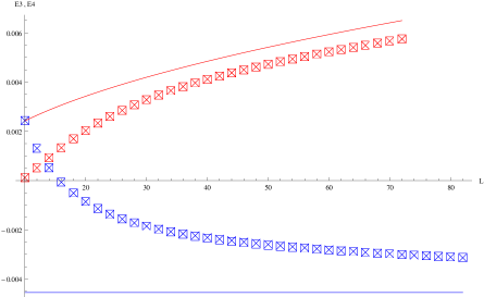 |
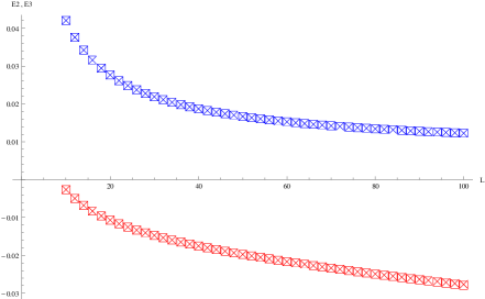
|
VI Concluding remarks: Towards a fluctuating Hydrodynamics description
In these lectures, we have explained that non-equilibrium processes can be explored by studying the large deviations of some physical observable such as the total current transported through a wire or the density profile. Indeed, large deviation functions appear to be to right generalization of the thermodynamic potentials to non-equilibrium systems. They exhibit remarkable properties such as the Fluctuation Theorem that is valid far away from equilibrium. Large deviation functions are likely to play a key-role in the future of non-equilibrium statistical mechanics.
The asymmetric exclusion process is a paradigm for non-equilibrium behaviour in low dimensions. Just as the Ising model for phase transitions, the ASEP is the simplest non-trivial model that embodies the minimal ingredients to study mathematically statistical physics far from equilibrium.
For the specific case of the ASEP, we have shown how large deviation function can be calculated exactly by using techniques borrowed from the theory of integrable systems, such as the Bethe Ansatz or the Matrix Representation method. The results obtained are exact and mathematically appealing, but the calculations required are rather involved and can only be applied to very specific models. It would be highly desirable to have at our disposal a more physical picture and a a set of tools more versatile that would allow us to study very general non-equilibrium systems.
It seems that such a theory has been emerging in the recent years. This approach is based upon a fluctuating hydrodynamic description. As a conclusion of these lectures, we shall briefly describe this theory and its relation to the problems studied here.
We consider again a diffusive system in contact with two reservoirs and we adopt the hydrodynamic description of Figure 16 consider the case with no applied field On average, the evolution of the profile and the current is governed by Burgers equation (19). But, what if we are interested in stochastic properties of the profile and the current? Suppose we want to know the probability to observe an atypical current and the corresponding density profile during ? For many systems, this probability will follow a large deviation behaviour:
(This is highly non-trivial. We simply assume it here). The functional is the large deviation functional.
For driven diffusive systems, G. Jona-Lasinio and coworkers have developed a formalism to calculate , known as the Macroscopic Fluctuation Theory (MFT) (see Bodineau ; DerrReview ; Bertini for reviews). The goal is to replace the deterministic Burgers equation by a stochastic equation that describes correctly the fluctuations of the system in the diffusive scaling limit of large systems and long times. We shall formulate the MFT using once again the pipe model language: Consider the total number of particles transferred from the left reservoir to the right reservoir during time . Then one has
-
•
for small
-
•
for and .
where the two ‘phenomenological’ coefficients encode the value of the average current and its quadratic fluctuations. For the symmetric exclusion process, they are given by
The stochastic equation of motion is obtained as
where is a Gaussian white noise with variance
If we discard the noise term, we recover the Burgers equation (19). The important fact is that in the Macroscopic limit, fluctuations are accurately described by a multiplicative Gaussian white noise, the amplitude of this noise being proportional to the conductivity . Besides, the fact that this noise is vanishing small (its amplitude has a factor) will allow us to use saddle point/WKB methods.
Indeed, the equation of fluctuating hydrodynamics allows us to express the large-deviation functional as a path-integral. Since the current and the density evolve according to a stochastic dynamics, the weight of a trajectory between 0 and can be written as
In the large limit, the integral will be dominated by the optimal value of the exponent (saddle-point). Hence, the large deviation functional can be written as the solution of an optimal path problem:
| (89) |
with the constraint: Then, knowing one can deduce (by the contraction principle Touchette ) the LDF of the current or the profile. For example, for the current:
This variational problem (89) has a Hamiltonian structure and can be expressed by using a pair of conjugate variables . Mathematically, one has to solve the corresponding Euler-Lagrange equations. After some transformations, a set of coupled non-linear PDEs is obtained:
where is the density-field and is a conjugate field. These equations have to be completed by suitable boundary conditions. We emphasize that this formalism can be applied to general diffusive systems: Physics is embodied in the transport coefficients and that carry the information of the microscopic dynamics relevant at the macroscopic scale.
In principle, the MFT provides us with a general framework but the non-linear PDEs obtained are very difficult to solve in general. If we can solve them, we should be able to calculate large deviation functions directly at the macroscopic level, without having to cope with the intricate combinatorics at the microscopic scale. For the moment being, very few solutions of these equations exist. The exact results we have described in these lectures can be used as benchmarks for the analysis of this new set of hydrodynamic equations, a field of research that has just opened.
References
- (1) R. J. Baxter, 1982 Exactly solvable models in Statistical Mechanics (Academic Press, San Diego).
- (2) L. Bertini, A. De Sole, D. Gabrielli, G. Jona-Lasinio and C. Landim, 2002, Macroscopic Fluctuation Theory for stationary non-equilibrium states, J. Stat. Phys. 107, 635.
- (3) R. A. Blythe and M. R. Evans, 2007, Nonequilibrium steady states of matrix-product form: a solver’s guide, J. Phys. A: Math. Theor. 40, R333.
- (4) T. Bodineau, B. Derrida, 2007, Cumulants and large deviations of the current through non-equilibrium steady states, C. R. Physique 8, 540.
- (5) D. Chowdhury, A. Schadschneider and K. Nishinari, 2005 Physics of transport and traffic phenomena in biology: from molecular motors and cells to organisms, Phys. Life Rev. 2, 318.
- (6) T. Chou, K. Mallick and R. K. P. Zia, Non-equilibrium Statistical Mechanics: from a paradigmatic model to biological transport, Rep. Prog. Phys. 74, 116601 (2011).
- (7) B. Derrida, 2007, Non-equilibrium steady states: fluctuations and large deviations of the density and of the current, J. Stat. Mech.: Theor. Exp. P07023.
- (8) B. Derrida, Microscopic versus macroscopic approaches to non-equilibrium systems, J. Stat. Mech. P01030 (2011).
- (9) B. Derrida, M. R. Evans, V. Hakim, V. Pasquier, 1993, Exact solution of a 1D asymmetric exclusion model using a matrix formulation, J. Phys. A: Math. Gen. 26, 1493.
- (10) B. Derrida, J. L. Lebowitz, 1998, Exact large deviation function in the asymmetric exclusion process, Phys. Rev. Lett. 80, 209.
- (11) D. Dhar, 1987, An exactly solved model for interfacial growth, Phase Transitions 9, 51.
- (12) G. Gallavotti, E. G. D. Cohen, 1995 Dynamical ensembles in non-equilibrium statistical mechanics, Phys. Rev. Lett. 74, 2694.
- (13) O. Golinelli, K. Mallick, 2006, The asymmetric simple exclusion process : an integrable model for non-equilibrium statistical mechanics, J. Phys. A: Math. Gen. 39, 12679.
- (14) M. Gorissen, A. Lazarescu, K. Mallick and C. Vanderzande, 2012, Exact Current Statistics of the Asymmetric Simple Exclusion Process with Open Boundaries, Phys. Rev. Lett. 109, 170601.
- (15) L.-H. Gwa, H. Spohn, 1992, Bethe solution for the dynamical-scaling exponent of the noisy Burgers equation, Phys. Rev. A 46, 844.
- (16) T. Halpin-Healy, Y.-C. Zhang, 1995, Kinetic roughening phenomena, stochastic growth, directed polymers and all that, Phys. Rep. 254, 215.
- (17) S. A. Janowski, J. L. Lebowitz, 1992 Finite size effects and Shock fluctuations in the asymmetric exclusion process, Phys. Rev. A 45, 618; S. A. Janowsky and J. L. Lebowitz, 1994, J. Stat. Phys. 77, 35 (1994); O. Costin, J. L. Lebowitz, E. R. Speer, and A. Troiani, arXiv:1207.6555.
- (18) S. Katz, J. L. Lebowitz, H. Spohn, 1984, Nonequilibrium steady states of stochastic lattice gas models of fast ionic conductors, J. Stat. Phys. 34, 497.
- (19) P. L. Krapivsky, S. Redner and E. Ben-Naim, 2010, A Kinetic View of Statistical Physics (Cambridge: Cambridge University Press).
- (20) T. Kriecherbauer and J. Krug, 2010, A pedestrian’s view on interacting particle systems, KPZ universality and random matrices, J. Phys. A: Math. Theor. 43, 403001.
- (21) C. MacDonald, J. Gibbs, and A. Pipkin, Kinetics of biopolymerization on nucleic acid templates, Biopolymers 6, 1 (1968); C. MacDonald and J. Gibbs, Concerning the kinetics of polypeptide synthesis on polyribosomes, Biopolymers 7, 707 (1969).
- (22) J. L. Lebowitz, H. Spohn, 1999 A Gallavotti-Cohen type symmetry in the large deviation functional for stochastic dynamics, J. Stat. Phys. 95, 333.
- (23) S. Prolhac, 2010, Tree structures for the current fluctuations in the exclusion process, J. Phys. A: Math. Theor. 43, 105002.
- (24) T. Sasamoto, 2007, Fluctuations of the one-dimensional asymmetric exclusion process using random matrix techniques, J. Stat. Mech.: Theor. Exp. P07007.
- (25) A. Schadschneider, D. Chowdhury and K. Nishinari Stochastic Transport in Complex Systems: From Molecules to Vehicles, (Amsterdam: Elsevier, 2011).
- (26) B. Schmittmann and R. K. P. Zia, 1995, Statistical mechanics of driven diffusive systems, in Phase Transitions and Critical Phenomena vol 17., C. Domb and J. L. Lebowitz Ed., (San Diego, Academic Press).
- (27) H. Spohn, Large Scale Dynamics of Interacting Particles (New York: Springer-Verlag, 1991).
- (28) H. Touchette, 2009, The large deviation approach to statistical mechanics, Phys. Rep. 478 1.
- (29) N. G. Van Kampen, 2007 Stochastic Processes in Physics and Chemistry, (North-Holland, Third Edition).